Integrating BIM and Machine Learning for Energy and Carbon Performance Prediction in Office Building Design

Abstract

Accurate early-stage assessment of building energy and carbon performance is essential for informed sustainable design yet remains challenging due to limited design detail and simulation effort. This study presents a Building Information Modeling–Machine Learning (BIM-ML) framework for predicting office building energy and carbon performance at early design stages using simulation-based datasets. A reduced-factorial Design of Experiments (DOE) generated 210 parametric office building models for Orlando, Florida (ASHRAE Climate Zone 2A), complemented by additional climate scenarios. Systematic variations in geometry, envelope, building systems, and operational schedules produced a dataset with 14 independent variables and five performance indicators: Energy Use Intensity, Operational Energy, Operational Carbon, Embodied Carbon, and Total Carbon. Four regression methods—Linear Regression, Model Tree (M5P), Sequential Minimal Optimization Regression, and Random Forest—were trained and evaluated using 10-fold cross-validation. Random Forest showed the strongest overall predictive performance. Feature-importance analysis identified HVAC system type, Window-to-Wall Ratio, and operational schedule as the most influential parameters, while geometric factors had lower impact. Cross-climate analysis and validation with measured data from two university office buildings indicate that the framework is adaptable and generalizable, supporting reliable early-stage evaluation of energy and carbon performance.

1. Introduction

Buildings have large energy consumption and are responsible for about 37% of global CO₂ emissions [1]. As cities continue to grow and technology becomes more central to daily life, energy demand keeps increasing, especially in office buildings that have extended operations and depend heavily on mechanical cooling and ventilation. Reducing these impacts requires design choices that lower energy use from operation and consider the carbon footprint linked to building materials and construction.

Most of these decisions are made very early in the design process, when the building’s form, envelope, systems, and typical use patterns are first defined. Because these early choices strongly influence long-term performance, evaluating energy and carbon impacts at this stage is one of the most effective ways to guide projects toward lower-emission outcomes and support broader climate-reduction goals.

1.1. Energy and Carbon Prediction Assessment Approaches

Traditional building-performance assessments rely on engineering calculations and simulation tools that model heat transfer, HVAC operation, and other physical processes. Seyedzadeh et al. [2] group these methods into four categories: engineering models, simulation tools, statistical models, and Machine Learning (ML) approaches.

Engineering and simulation tools, such as EnergyPlus (v9.6.0), eQuest (v3.65build7175), and DesignBuilder (v6.1.8.021), are detailed and accurate, but require extensive inputs, long run times, and specialized expertise. These demands make them difficult to use during early design, when many options must be tested quickly. As a result, performance analysis is often postponed, reducing opportunities to guide projects toward lower-energy, lower-carbon solutions.

Statistical models help simplify this process by identifying patterns in historical or measured data. Techniques such as regression, Artificial Neural Networks (ANNs), and Support Vector Machines (SVMs) have shown good accuracy in forecasting short and long-term energy use with fewer inputs [3,4]. Their success illustrated an early shift toward data-driven prediction.

With greater computing power and larger datasets, ML methods have become more common in building analysis. Recent studies (e.g., Duarte et al. [5]) show that ML models trained on simulation data can estimate energy loads and Energy Use Intensity (EUI) quickly and reliably. Because building performance depends on nonlinear interactions among envelope properties, HVAC efficiency, occupancy schedules, geometry, and Lighting Power Density (LPD) [5,6], algorithms such as Random Forest (RF) and SVM often outperform simpler statistical models [7]. These ML surrogates allow rapid performance screening during early design. Recent review studies further emphasize that key challenges for broader adoption include dataset quality, model generalization beyond the training domain, and the interpretability of ML predictions for design decision-making [8,9].

Energy analysis alone, however, does not capture the full environmental impact of buildings. Operational Carbon (OC) represents emissions from Operational Energy use, while Embodied Carbon (EC) reflects emissions from material production, transport, and construction. Together, they form Total Carbon (TC), a key life-cycle indicator [10]. OC depends largely on system efficiency and grid carbon intensity, whereas EC is shaped by material choices and supply-chain processes.

Carbon assessment traditionally relies on Life Cycle Assessment (LCA), but LCA is data-heavy and time-consuming, often impractical during conceptual design. Data-driven and ML-based carbon models address this gap by providing faster estimates and enabling early comparison of design strategies. Recent studies demonstrate that Machine Learning approaches can successfully predict embodied or total carbon emissions during conceptual design when detailed LCA inputs are unavailable [11,12,13].

Studies such as Nwodo and Anumba [14] demonstrate that supervised ML models—such as Liner Regression (LR), RF and ANN—can approximate life-cycle emissions well when trained on reliable datasets. Hong et al. [15] highlights that ML can improve LCA scalability and reduce manual inputs, while also noting that carbon predictions must reflect local or regional emission factors to remain valid across different contexts.

Research has increasingly emphasized the value of integrating carbon analysis from the beginning of design. Work by Feng et al. [16], Zhang and Sandanayake [17], and Gan et al. [18] shows that BIM combined with ML and optimization can evaluate embodied and operational impacts simultaneously. Pan et al. [19] further demonstrate that BIM-based workflows help track these impacts across the project life cycle.

Overall, existing studies show that predicting both energy and carbon performance early in the design process is essential for low-impact decision-making. This supports the motivation for the present study, which uses BIM-generated simulation data and ML surrogate models to estimate energy and carbon outcomes efficiently during early design.

1.2. Machine Learning for Performance Prediction

ML has become an effective way to speed up building-performance evaluation by learning patterns from simulation results and using them to predict outcomes without running new simulations each time. Once trained, ML models can estimate metrics such as energy use or carbon emissions in seconds, making them especially useful during early design when many alternatives must be tested quickly [6]. Recent studies show that integrating ML directly with BIM environments enables practical early-stage decision support while significantly reducing the computational burden associated with repeated simulations [20].

ML techniques are commonly grouped into supervised, unsupervised, and hybrid methods [2]. In building-performance prediction, supervised learning is the most widely used because it connects known inputs—geometry, envelope features, HVAC type, and operating schedules—to measured or simulated outputs. Algorithms often applied in this context include LR, RF, Model Tree (M5P), and Sequential Minimal Optimization Regression (SMOReg), each offering different strengths [3,5]:

• LR provides simple and transparent relationships between features and outputs;
• RF and M5P handle nonlinear interactions and mixed variable types; and
• SMOReg, an implementation of Support Vector Regression (SVR), adapts well to complex datasets through kernel functions.

Although unsupervised learning is less common for direct prediction, it can support tasks such as identifying clusters of similar building configurations or detecting irregularities in energy datasets. Hybrid approaches combine multiple techniques to improve accuracy or handle diverse data sources.

Surrogate models, lightweight predictors trained on detailed simulation results, are increasingly used to replace time-consuming physics-based analyses. Studies such as Robinson et al. [21] and Geyer & Singaravel [22] show that ML-based surrogates can reproduce key performance indicators with high accuracy using relatively few inputs. More recent surrogate model studies confirm strong predictive performance across multiple targets and highlight their effectiveness for early-stage design-space exploration [23].

Kim et al. [24] demonstrated that pairing parametric modeling with neural networks helps explore design variations efficiently, while Rahmani et al. [25] found that BIM-derived data provides consistent geometric and material information that improves model reliability. Because the “black-box” nature of ML models remains a concern in practice, recent research increasingly focuses on interpretable and explainable ML techniques to improve trust and usability in design decision-making [26].

Beyond energy prediction, recent work has extended ML methods to carbon estimation. Research by Nwodo and Anumba [14] and D’Amico et al. [27] shows that models trained on BIM-extracted attributes, such as material quantities, façade areas, and structural components, can estimate EC and other life-cycle impacts effectively. These studies highlight the value of integrating both energy and carbon prediction into unified ML workflows, an approach further developed in this study to support early sustainable-design decisions.

1.3. Integration of Building Information Modeling and Machine Learning

Building Information Modeling (BIM) supports the creation of coordinated 3D models that contain geometry, materials, and system information needed for performance analysis. Platforms such as Autodesk Revit and Autodesk Insight allow designers to assess energy and carbon impacts earlier and more efficiently, improving communication across project teams.

Because BIM stores detailed spatial and semantic information in a structured format, it provides a reliable source of inputs for ML. This organization makes it possible to generate consistent datasets directly from the design model, linking building parameters to simulated performance outcomes without extensive manual rework.

Several studies have explored how BIM and ML can work together to enhance sustainability evaluations. For example, Ma et al. [28] developed a BIM-ANN plug-in that delivered quick feedback on energy and comfort performance, showing how predictive models can be embedded into the design workflow. Other researchers, including Holberg et al. [29], point out persistent challenges, such as fragmented data formats and limited shared repositories, that restrict broader adoption of BIM-ML workflows.

Khan et al. [30] identified interoperability issues as a major barrier, noting that inconsistent data structures and non-standard workflows often complicate the exchange of information between BIM tools and ML platforms. Meng et al. [31] added that organizational and policy factors also influence whether BIM-based sustainability tools are used effectively in practice. These findings highlight the need for practical, simplified workflows that reduce data-preparation effort and make BIM-ML integration easier to adopt.

Integrating ML directly into BIM-centered processes enables rapid prediction of performance metrics, allowing multiple design alternatives to be tested with minimal computation. Pan et al. [19] showed that BIM-ML approaches can support continuous evaluation throughout a project, improving the clarity of design decisions. Building on this foundation, the present study develops a BIM-derived dataset and ML surrogate models capable of predicting both energy and carbon outcomes, strengthening the connection between digital modeling and sustainability-focused design.

1.4. Addressing Uncertainty and Early Design Stages

Predicting building performance early in design is challenging because many key parameters, such as geometry, material choices, operating schedules, and occupant behavior, are not yet fully defined. These uncertainties can lead to wide variations between projected and actual outcomes. Ning and You [32] highlight that overcoming this issue requires automated methods that can evaluate many design options quickly, helping designers explore a broader solution space even when information is limited.

Several studies propose combining parametric modeling with ML to better handle early-stage uncertainty. Feng, Lu, and Wang [16] showed that linking parametric tools with predictive models allows systematic testing of how variable inputs affect energy and carbon performance, helping identify which parameters have the greatest impact. Walker et al. [33] further demonstrated that prediction accuracy depends on the resolution of the data—hourly, daily, or annual—suggesting that model detail should match the design question being addressed.

Research has also shown that evaluating energy and carbon together can improve reliability. While earlier work by Zhang and Sandanayake [17] focused on certification contexts, more recent studies [15] confirm that joint modeling captures relationships between these indicators more effectively than treating them separately.

Within a BIM environment, uncertainty can be reduced by generating controlled parametric variations and simulating each configuration. This approach produces structured datasets with consistent inputs and outputs, allowing ML models to learn from a wide range of plausible design scenarios. The present study adopts this strategy to create a diverse, high-quality dataset for training and validating ML models that support early-stage sustainability decisions.

To clarify how existing methods differ in terms of data requirements, computational effort, early-stage applicability, and ability to predict both energy and carbon performance, Table 1 summarizes representative approaches reported in the literature. The comparison highlights the strengths and limitations of engineering-based, simulation-based, statistical, and Machine Learning methods, and positions integrated BIM-ML frameworks within the current research landscape, motivating the need for scalable and interpretable early-stage prediction approaches.

Table 1. Comparison of representative approaches for early-stage building energy and carbon performance prediction.

Approach	Typical Tools/Methods	Data Source	Strengths	Limitations	Representative Studies
Engineering calculations	ASHRAE hand calculations, simplified equations	Assumed or standard inputs	Transparent, low computational cost	Oversimplified; limited ability to capture nonlinear interactions; low accuracy for complex buildings	Kalogirou [4]
Physics-based simulation	EnergyPlus, DOE-2, eQuest, DesignBuilder	Detailed model inputs	High physical accuracy; industry accepted	Time-consuming; requires detailed inputs; impractical for early design iteration	Seyedzadeh et al. [2], Hong et al. [15]
Statistical models	Linear Regression, ANN, SVM	Measured or simulated data	Faster than simulation; moderate data needs	Limited generalization; sensitive to data quality; weak interpretability	Ahmad et al. [3], Fumo & Biswas [6]
ML on measured data	RF, ANN, SVR	Real building datasets	Captures real operational behavior	Limited availability of large, clean datasets; poor early-stage applicability	Robinson et al. [21], D’Amico et al. [27]
BIM-based simulation only	Revit + Insight	BIM-derived parametric simulations	Integrated with design workflow; consistent geometry	Still computationally expensive; limited decision-speed	Pan et al. [19], Gan et al. [18]
Integrated BIM + ML (prior studies)	BIM platforms (e.g., Revit) + ML models (e.g., RF, ANN, regression-based surrogates)	BIM-based simulated datasets	Enables early-stage performance prediction; captures nonlinear relationships; improves decision support compared to standalone simulation	Often limited to specific building types or climates; reduced parameter scope; limited validation across large design spaces	Feng et al. [16], Singh et al. [20]
Integrated BIM + ML framework (this study)	Revit + Insight + ML surrogates	BIM-based simulated dataset	Fast early-stage prediction; captures nonlinear effects; interpretable; scalable; compatible with BIM-based design workflows	Dependent on simulation assumptions; requires regional carbon calibration	This study.

The table summarizes representative approaches for predicting building energy and carbon performance, with emphasis on early-stage design applicability. It highlights the limitations of standalone simulation and data-driven methods and the advantages of integrating BIM-generated simulation data with Machine Learning surrogates. The final row corresponds to the BIM-ML framework proposed in this study.

1.5. Research Gap and Study Objectives

Although ML has become increasingly common in building performance prediction, several barriers still limit its use in everyday practice. One recurring concern is the “black-box” nature of many algorithms, which makes it difficult for designers to understand how predictions are generated [15]. This lack of interpretability, combined with the strong dependence of ML models on training-data quality, can lead to issues such as overfitting and inconsistent results across projects [34].

A major challenge highlighted in recent studies is the limited availability of structured, high-quality datasets. Holberg, Genova, and Habert [29] noted that the absence of standardized BIM-based energy and carbon data restricts model validation and reduces confidence in predictive outcomes. D’Amico et al. [27] similarly emphasized the need for shared datasets that capture a broad range of design parameters, which would enable more reliable comparison and benchmarking of ML methods.

Technical and workflow constraints also hinder smooth integration between BIM and ML. Pan et al. [19] pointed out that non-uniform modeling practices and fragmented data flows disrupt continuity between tools. Other reviews, such as Khan et al. [30] and Meng et al. [31], show that interoperability problems, inconsistent data schemas, and organizational factors further slow progress toward widespread adoption.

Even with these challenges, recent research demonstrates that ML-based surrogate models can offer fast and accurate performance estimates, reducing reliance on repeated simulation runs. Building on this potential, the present study develops a unified predictive framework that evaluates both energy and carbon outcomes using BIM-generated data and ML models. This approach addresses the documented gaps in data structure, interoperability, and early-design assessment, while supporting more efficient and scalable sustainability analysis.

2. Materials and Methods

This study established a BIM-ML workflow to support early-stage prediction of building energy use and carbon emissions. The process combined Autodesk Revit 2024 for generating geometric models, Autodesk Insight 2023.1 for running parametric simulations and extracting performance data, and Weka for ML training and evaluation. The workflow was structured to be clear, repeatable, and adaptable so it can be applied consistently during conceptual design. Figure 1 provides an overview of the BIM-ML workflow adopted in this study, which is detailed in the following subsections.

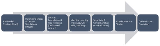
Figure 1. Overall BIM-ML study methodology workflow, illustrating the sequence from BIM model generation and parametric simulation-based dataset creation to Machine Learning training, sensitivity analysis, validation, and carbon factor correction.

2.1. Overall Research Framework and Methodology

A reduced-factorial Design of Experiments (DOE) method [35,36] was used to organize the simulation plan. This approach allowed broad exploration of key design variables while keeping the total number of simulations manageable. In total, 210 building models were created and grouped into three sets:

• 168 base models: core combinations of the main design parameters;
• 32 generalization models: supplemental variations added to expand parameter coverage and strengthen model generalization; and
• 10 stress-test models: extreme cases used to evaluate how well predictions are held under atypical conditions.

Each model reflected a distinct combination of geometric, envelope, system, and operational parameters. This structure provided sufficient coverage of main effects and interactions, supporting reliable training and validation of the ML models.

Although the model incorporates 11 input variables, the resulting dataset of 210 samples provides approximately 19 samples per variable, which is consistent with commonly accepted practices for regression and tree-based Machine Learning models. The selected algorithms (LR, RF, M5P, and SMOReg) are well suited to small-to-moderate tabular datasets and have been widely applied in building-performance prediction studies with comparable or smaller sample sizes. Model adequacy was further verified through cross-validation and multiple performance standard statistical metrics—Coefficient of Determination (R²), Root Mean Square Error (RMSE), and Mean Absolute Error (MAE)—confirming that the dataset size was sufficient to support stable training and reliable prediction.

2.1.1. Experimental Parameters and Levels

The selection of experimental parameters and their corresponding levels was guided by three main criteria: (i) documented influence on early-stage building energy and carbon performance, (ii) compatibility with conceptual-design decision-making, and (iii) alignment with typical ranges reported in the building-performance literature and professional standards. Variables such as building geometry, orientation, HVAC system type, Window-to-Wall Ratios (WWR), Lighting Power Density (LPD), infiltration rate, plug loads, and operation schedules are consistently identified as primary drivers of office-building energy use and emissions, particularly in warm–humid climates [5,6,7,10,16,21].

Parameter ranges were constrained to represent realistic design choices for contemporary U.S. office buildings and to avoid extreme or nonstandard configurations that are unlikely to be considered during early design. Upper bounds for infiltration and LPD were selected to reflect common commercial practice and ASHRAE-compliant performance targets, while HVAC system options were limited to systems commonly deployed in mid-rise office buildings. Operation schedules were simplified into three representative patterns to capture typical, extended, and continuous-use scenarios without introducing excessive complexity.

Several parameters, including building lifespan, gross floor area range, and baseline emission factors, were held constant to isolate the effects of design and operational variables and to maintain comparability across simulations. This controlled parameter selection ensured statistical consistency within the reduced-factorial DOE framework while preserving relevance to real-world early-stage design conditions.

Although building envelope assemblies (external walls, roofs, and windows) play a critical role in determining building energy and carbon performance, they were represented in this study at an aggregate performance level consistent with early-stage design practice and the abstraction level supported by Insight. Rather than explicitly parameterizing detailed material-layer assemblies, envelope performance was captured through effective thermal properties and system-level inputs, including WWR, glazing type, Solar Heat Gain Coefficient (SHGC), and code-compliant baseline constructions for opaque elements.

External wall and roof constructions were held constant across simulations using standard assemblies consistent with ASHRAE 90.1 requirements for Climate Zone 2A, allowing the analysis to focus on design variables more commonly adjusted during conceptual stages. This approach reduces dimensionality within the reduced-factorial DOE while maintaining physical realism and comparability across cases. The selected representation aligns with prior BIM-based parametric and machine-learning studies that prioritize envelope performance indicators over detailed material definitions during early design. Accordingly, envelope assemblies were treated as fixed baseline conditions rather than independent experimental variables in the DOE.

The experimental setup included 11 independent variables representing the main design and operational factors that influence early-stage energy and carbon performance. These parameters covered building shape, orientation, HVAC system type, infiltration rate, LPD, operation schedule, plug loads, and WWR for each façade (North, East, South, and West).

To maintain consistency across simulations, several conditions were fixed. Building lifespan was set to 20 years, and a uniform emission factor of 0.45 kg CO₂e/kWh was applied. All prototypes were also kept within a similar Gross Floor Area (GFA) range (approximately 27,000–31,000 ft²) to ensure comparability and minimize scale effects.

Although Insight offers many default settings, the number of levels per parameter was intentionally limited. The goal was to preserve the statistical structure of the reduced-factorial design, control computational effort, and ensure that each level represented a realistic design choice for office buildings in warm–humid climates.

HVAC systems not commonly used in this building type, such as radiant floors, evaporative cooling, or district cooling, were excluded. Upper limits were also applied to infiltration (≤0.12 CFM/ft²) and LPD (≤1.00 W/ft²) to reflect typical ranges for contemporary commercial buildings. Operation schedules were narrowed to three representative patterns (8 a.m.–5 p.m., 12/5, and 24/7), capturing standard, extended, and continuous use.

As shown in Table 2, the parameters contained unequal numbers of levels (7, 4, 4, 3, 3, 3, 2, 3, 3, 3, and 3). Under a full-factorial design, this would produce more than 1.6 million possible combinations, underscoring the importance of adopting a reduced-factorial strategy.

Table 2. Experimental parameters and corresponding levels used in the reduced-factorial design.

Parameter	Number of Levels	Levels
Shape	7	Square, Rectangular, Cross, L, U, H, and T
Orientation (°)	4	0, 45, 90, 180
HVAC System	4	Base by Design, VAV w/WC and Gas, VAV w/WC and EB, GSHP w/DOAS + ERV *
Infiltration Rate (CFM/ft2)	3	0.04, 0.09, 0.12
LPD (W/ft2)	3	0.45, 0.72, 1.00
Operation Schedule	3	8 a.m.–5 p.m., 12/5, 24/7
Plug Loads (W/ft2)	2	1.0, 1.3
WWR East (%)	3	0, 30, 50
WWR North (%)	3	0, 30, 50
WWR South (%)	3	0, 30, 50
WWR West (%)	3	0, 30, 50

Adapted from the author’s dissertation [37]. * Note: Base by Design refers to the default HVAC baseline system automatically assigned by Insight when no custom configuration is specified. This system represents the platform’s internally defined reference case used to ensure energy model functionality and comparability across simulations. In this study, it served as the control case for benchmarking the three explicitly defined systems—VAV w/WC and Gas, VAV w/WC and EB, and GSHP w/DOAS + ERV.

2.1.2. Reduced-Factorial Framework

To efficiently sample the design space without the prohibitive size of a full-factorial experiment, a custom reduced-factorial plan was created in Microsoft Excel. The final dataset (N = 168) provided balanced representation across all 11 parameters and maintained compatibility with the principal level counts (7, 4, 3, and 2). This ensured broad coverage of geometric, envelope, system, and operational variations while keeping the number of Revit-Insight simulations manageable.

Two constraints were applied to preserve architectural realism and avoid implausible combinations:

• HVAC–orientation matching: only feasible system-orientation pairs were permitted (e.g., GSHP w/DOAS + ERV for 0–45°, and VAV w/WC systems for 90–180°); and
• Façade WWR coordination: glazing configurations were limited to nine predefined patterns (e.g., [0, 0, 0, 0], [30, 30, 30, 30], and [50, 50, 50, 50]) to ensure coherent façade designs.

To evaluate the independence of the predictors, a correlation matrix was generated using numerically encoded categorical variables. Except for the intentional couplings (HVAC–orientation and façade-pattern rules), all pairwise correlations were below |0.35|. This confirmed that the reduced-factorial structure avoided multicollinearity and preserved sufficient orthogonality for ML analysis. The full matrix is shown in Table 3.

Table 3. Correlation matrix for the 11 simulation predictors (N = 168 reduced-factorial configurations).

Predictor	Shape	Orient.	HVAC	Infilt.	LPD	Schedule	Plug Load	WWR E	WWR N	WWR S	WWR W
Shape	1.00	0.04	0.06	−0.02	−0.03	−0.02	0.02	−0.07	−0.06	−0.06	−0.02
Orientation	0.04	1.00	0.70	−0.13	−0.02	0.04	0.32	−0.52	−0.72	−0.07	0.01
HVAC System	0.06	0.70	1.00	−0.37	−0.22	0.07	0.20	−0.72	−0.60	−0.39	−0.28
Infiltration	−0.02	−0.13	−0.37	1.00	−0.02	−0.03	0.01	0.08	0.06	−0.03	−0.02
LPD	−0.03	−0.02	−0.22	−0.02	1.00	−0.09	0.00	0.17	0.10	−0.04	−0.37
Schedule	−0.02	0.04	0.07	−0.03	−0.09	1.00	0.71	−0.01	0.05	0.61	0.61
Plug Loads	0.02	0.32	0.20	0.01	0.00	0.71	1.00	0.24	0.19	0.34	0.63
WWR East	−0.07	−0.52	−0.72	0.08	0.17	−0.01	0.24	1.00	0.80	0.23	0.02
WWR North	−0.06	−0.72	−0.60	0.06	0.10	0.05	0.19	0.80	1.00	0.43	0.23
WWR South	−0.06	−0.07	−0.39	−0.03	−0.04	0.61	0.34	0.23	0.43	1.00	0.80
WWR West	−0.02	0.01	−0.28	−0.02	−0.37	0.61	0.63	0.02	0.23	0.80	1.00

Based on reduced-factorial DOE dataset. Adapted from the author’s dissertation [37].

Level-balance checks compared to the actual versus expected frequency of each parameter level (ideal = N/number of levels). Deviations remained within an acceptable ±12-run range for all factors, indicating that the design met DOE criteria for approximate balance and independence.

The finalized reduced-factorial matrix served as the master input schedule for the Revit-Insight simulation sequence.

2.1.3. Dataset Expansion and Stress Testing

After training the first ML models using the 168 reduced-factorial cases, the dataset was expanded to improve diversity and strengthen generalization. A set of 32 additional generalization models (M-169 to M-200) was created by adding new combinations that respected all coupling rules and façade-pattern constraints while increasing the representation of levels that appeared less frequently in the base design.

To further test model robustness, 10 stress-test cases (M-201 to M-210) were developed to represent boundary conditions.

Five high-load scenarios combined elevated internal gains and envelope demands, using the upper limits for LPD (1.00 W/ft²), plug loads (1.3 W/ft²), infiltration (0.12 CFM/ft²), a continuous 24/7 schedule, and high-glazing façade patterns (WWR = [50, 50, 50, 50] or [50, 50, 0, 0]).

Five low-load scenarios applied the opposite conditions: minimum LPD (0.45 W/ft²), lower plug loads (1.0 W/ft²), reduced infiltration (0.04 CFM/ft²), a standard 8 a.m.–5 p.m. schedule, efficient HVAC (GSHP w/DOAS + ERV), and low-glazing façade patterns.

All expansion and stress-test models preserved the same shape-area mapping and parameter consistency used in the base runs. This ensured methodological continuity while broadening the range of conditions used for ML training and evaluation.

Through structured parameter variation, targeted dataset expansion, and controlled boundary testing, the final experimental design provided a comprehensive yet computationally manageable representation of the early-design solution space.

The resulting 210 unique Revit-Insight model configurations formed the complete dataset for subsequent ML-based energy and carbon prediction.

2.2. Model Development

Seven three-story office building prototypes were created in Revit to represent a range of common early-design geometries: square, rectangular, cross, L-shape, U-shape, H-shape, and T-shape. All models were designed with similar GFA (approximately 27,000–31,000 ft²) and uniform floor-to-floor heights to ensure that observed performance differences resulted from parameter changes rather than variations in size.

Each prototype was set to the climate and location of Orlando, Florida (ASHRAE Climate Zone 2A) [38], which was selected as the primary case study due to its cooling-dominated, warm–humid conditions and the high Operational Energy demand typically associated with office buildings in this climate. This context makes early-stage design decisions particularly influential on long-term energy and carbon performance. Revit’s analytical modeling tools were used to generate clean geometry and maintain compatibility with Insight.

To assess the adaptability of the proposed BIM–ML framework beyond a single climate, additional simulations were conducted for representative ASHRAE climate zones with contrasting thermal characteristics. These zones were selected to test the robustness and generalizability of the framework rather than to provide full climate-specific calibration across all U.S. climate zones.

Once the analytical models were prepared, they were exported to Insight, where physical, environmental, and operational parameters were assigned according to the experimental design. Insight then performed the energy and carbon simulations used to develop the dataset for ML prediction. Because the workflow relies on multiple base geometries and structured variation of analytical parameters within Insight, each base building geometry remains consistent across its simulation variants, while performance-related inputs are varied according to the experimental design.

2.3. Parametric Simulation

The simulation workflow combined Revit and Insight, with each platform responsible for different parts of the parametric setup. Revit controlled all geometric and location-based input, such as building shape, floor-to-floor height, site coordinates, and orientation, ensuring that the analytical model accurately reflected the intended form and solar exposure. Operational and system-related parameters were then assigned in Insight, which is optimized for adjusting HVAC settings, schedules, glazing ratios, and other performance variables.

Separating the parameters in this way helped maintain consistency across all model runs. Revit ensured that every geometric prototype followed identical rules and boundary conditions, while Insight handled the performance settings required for energy and carbon evaluation. This division reduced redundant modeling steps, improved traceability of design changes, and ensured that each parameter was adjusted within the environment best suited for its simulation role.

2.3.1. Revit Controlled Parameters

Revit managed the parameters that define each building’s physical form and environmental context. These variables shape the analytical geometry and set the boundary conditions used in subsequent simulations.

• Shape determined the overall footprint, façade distribution, and building volume, establishing the base envelope for energy and carbon analysis; and
• Location assigned the climate file, solar path, and weather data. These settings were taken directly from Revit’s project environment and passed automatically to Insight.

Because both factors influence geometric accuracy and solar exposure, they were configured entirely within Revit. This ensured that the analytical model imported into Insight correctly reflected each prototype’s spatial characteristics and climatic conditions.

2.3.2. Insight Controlled Parameters

All non-geometric parameters, including system settings, operational characteristics, and envelope performance, were assigned directly in Insight. Insight provides a parametric interface linked to DOE-2 [39] and EnergyPlus [40], allowing these variables to be modified efficiently while keeping the underlying analytical geometry fixed. The following parameters were controlled within Insight: HVAC system type, infiltration rate, LPD, plug loads, operation schedule, and façade-specific WWRs.

Managing these inputs in Insight avoided the need to create separate Revit files for each configuration, enabling rapid parameter variation consistent with the reduced-factorial design. For every model, the corresponding factor levels from the Excel-based experimental matrix were applied directly through Insight’s sliders and simulation settings.

Each simulation produced energy and carbon indicators used for ML training:

• Energy Use Intensity (EUI, kBtu/ft²·yr): building-level energy demand normalized by floor area;
• Operational Energy (OE, kBtu/yr): total projected annual energy consumption;
• Operational Carbon (OC, kgCO₂e/yr): annual emissions associated with Operational Energy use;
• Embodied Carbon (EC, kgCO₂e/yr): material-related emissions calculated using Insight’s baseline assumptions; and
• Total Carbon (TC, kgCO₂e/ft²): combined operational and embodied emissions normalized by GFA.

The outputs from all 210 Insight simulations were consolidated into a structured Excel database. Each row represented a unique building model along with its parameter values and associated performance results, forming the dataset used to train and validate the ML surrogate models.

2.4. Dataset Preparation

Performance data generated in Insight were exported to Excel, where all variables were checked for consistent units, naming conventions, and formatting. After cleaning, the dataset was converted into Attribute-Relation File Format (ARFF) using a plain-text editor to ensure compatibility with Weka’s ML environment.

The final ARFF file included 14 independent variables and five performance outputs: Energy Use Intensity (EUI), Operational Energy (OE), Operational Carbon (OC), Embodied Carbon (EC), and Total Carbon (TC). Categorical inputs—such as building shape, HVAC type, and operation schedule—were defined as nominal attributes, while continuous variables (e.g., infiltration rate, LPD, and WWR values) remained numeric to preserve their physical interpretation.

The dataset includes five performance outcomes extracted from Insight, representing key operational and environmental indicators relevant to early-stage building design. These metrics were selected because they are commonly used in both building-performance analysis and data-driven sustainability studies.

Annual Energy Use Intensity (EUI, kBtu/ft²·yr) represents total modeled Operational Energy consumption normalized by gross floor area and includes heating, cooling, ventilation, lighting, equipment, and auxiliary systems. Annual Operational Energy consumption is reported by the simulation engine as electricity (kWh) and natural gas (therms), enabling disaggregation by fuel type.

Operational Carbon emissions (kg CO₂e) are calculated by Insight based on annual energy consumption and region-specific emission factors for electricity and on-site fuel use. Carbon intensity (kg CO₂e/ft²·yr) represents normalized Operational Carbon emissions per unit floor area.

Embodied Carbon (kg CO₂e) represents material-related emissions associated with the building envelope and structural components, as estimated using Insight’s default material assumptions, while Total Carbon combines operational and embodied contributions over the defined analysis period. All performance outcomes were generated under consistent climate, schedule, and baseline assumptions to ensure comparability across design alternatives.

Additional performance indicators were also calculated to support carbon-focused analysis:

Numeric indices:

• Operational Carbon Performance Index (OCPI): expresses Operational Carbon efficiency relative to a standard baseline.
• Embodied Carbon Indicator (ECI₂₀): normalizes Embodied Carbon over a 20-year period, aligned with LEED material-efficiency benchmarks.
• Total Carbon Indicator (TCI₂₀): integrates Operational and Embodied Carbon over 20 years to evaluate overall carbon performance against LEED targets.

Categorical indices:

• Threshold-compliance flags (yes/no): indicate whether each model meets LEED-based goal and stretch targets. These thresholds, summarized in Table 4, serve as reference points for evaluating the relative performance of each configuration.
  Table 4. Threshold compliance metrics.

  Indicator	Goal Threshold (Minimum Compliance)	Stretch Threshold (High Performance)	Units
  EUI	≤45	≤35	kBtu/ft2·yr
  OPCI	≤12	≤8	kgCO2e/ft2.yr
  ECI20	≤30	≤20	kgCO2e/ft2
  TCI20	≤650	≤500	kgCO2e/ft2

  Adapted from LEED v4 [41] and Autodesk Insight (2024) reference metrics. Adapted from the author’s dissertation [37].

No additional normalization was required, as Weka’s algorithms perform internal scaling where appropriate. This structured dataset enabled consistent comparison of geometric, system, and operational effects on both energy and carbon outcomes.

2.5. Machine Learning Modeling

Four regression algorithms available in Weka were used to train and evaluate the predictive models: Linear Regression (LR), Model Tree (M5P), Sequential Minimal Optimization Regression (SMOReg) with polynomial and Radial Basis Function (RBF) kernels, and Random Forest (RF). These algorithms were selected to represent a range of linear, tree-based, kernel-based, and ensemble learning strategies commonly applied in building-performance research.

Each model was assessed using 10-fold cross-validation to provide an unbiased estimate of predictive accuracy. Performance was measured using three standard statistical indicators: R², RMSE, and MAE.

To understand how each input variable contributed to the predictions, feature-importance analysis was conducted using Weka’s ClassifierAttributeEval with the Ranker method, applying RF as the evaluation learner. This procedure quantified the relative influence of geometric, envelope, system, and operational parameters across all energy and carbon metrics, supporting model interpretability and guiding the discussion of design sensitivity.

2.6. Climate Analysis

To examine how different climates influence energy and carbon outcomes, and to determine whether performance thresholds would shift under varying environmental conditions, five additional U.S. cities were selected to represent a range of ASHRAE [38] climate zones. These locations cover diverse thermal and humidity profiles, as illustrated in Figure 2 and summarized in Table 5.

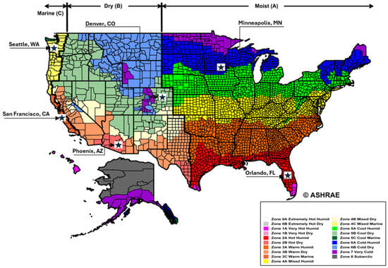
Figure 2. U.S. climate zones map with studied city locations. Adapted from ASHRAE Standard 169 (2013) [42], Climate Zones for United States Counties. Map accessed via ICC Digital Codes. Note: The map was modified by the author to indicate the six study locations (Orlando, San Francisco, Minneapolis, Phoenix, Denver, and Seattle). Adapted from the author’s dissertation [37].

Table 5. Climate variation test summary.

City	ASHRAE Zone	Climate Type	Number of Test Models	Purpose
Orlando, FL	2A	Hot/Humid	10	Baseline stress test and final model training
San Francisco, CA	3C	Marine	10	Contrast with mild marine climate
Minneapolis, MN	6A	Cold/Humid	10	Evaluate heating-dominated performance
Phoenix, AZ	2B	Hot/Dry	10	Assess cooling-dominant conditions
Denver, CO	5B	Cold/Dry	10	Examine altitude and low-humidity influence
Seattle, WA	4C	Cold/Marine	10	Test marine–cold mixed climate behavior

Based on ASHRAE Standard 169 (2013) [42] climate zone classification. Adapted from the author’s dissertation [37].

For each city, ten Revit-Insight simulations were generated using the same parameter settings applied to the Orlando stress-test models (M-201 to M-210). By holding all design variables constant and substituting only the weather files, the analysis isolates the effect of local climate on predicted energy and carbon performance.

The resulting climate-sensitivity dataset (50 models) was used exclusively for comparison across climates. These simulations were not included in ML training to ensure that the surrogate model remained calibrated specifically to Orlando conditions, while still enabling interpretation of how results might change in other regions. This allowed evaluation of whether LEED-related energy and carbon thresholds shift meaningfully when applied to different climates and revealed the limits of applying Orlando-trained predictions beyond warm–humid contexts.

Combining the primary 210-model Orlando dataset with the additional 50 climate-test simulations provided a stronger basis for understanding both predictive stability and climate-driven variability. This separation between the calibrated dataset (Orlando) and the exploratory dataset (cross-climate) also improved methodological clarity and prevented unintended generalization in ML model training.

2.7. Case Study Validation Methodology

To assess how well the ML surrogate models perform in real design contexts, the final evaluation was carried out using two existing LEED Gold-certified buildings on the University of Central Florida (UCF) main campus in Orlando, Florida (ASHRAE Climate Zone 2A). These facilities were selected because they share key characteristics with the simulated prototypes, a three-story configuration and an office-type program. Using buildings with similar scale and functional profiles ensured that the validation tested the surrogate models under conditions aligned with those represented in the training dataset, reducing mismatches related to geometry or operational patterns and providing a realistic measure of predictive performance.

2.7.1. Selection Rationale and DOE Alignment

The validation phase followed the same DOE logic used in the simulation plan by selecting a small number of real buildings that represent the main functional types modeled in this study. Rather than attempting to cover every possible building condition, the objective was to test whether the surrogate model produced reliable predictions for representative cases that fall within the study’s design space.

Two LEED Gold buildings on the UCF campus were selected for this purpose:

• UCF Global, an administrative office building with typical weekday occupancy and standard HVAC zoning; and
• UCF Research I, an academic office and research facility characterized by higher internal gains and greater plug-load intensity.

These buildings share similar heights and overall proportions to the three-story prototypes used in the simulations and operate with HVAC systems comparable in type and efficiency to those included in the DOE. While their exact glazing configurations were not modeled, the use of representative WWRs in the simulations provided a reasonable basis for comparison. This alignment allowed the trained ML model to be evaluated against actual performance data while keeping geometric and operational differences to a minimum.

2.7.2. Data Sources for Validation

Energy-performance data for the two UCF case-study buildings were obtained from the university’s Utilities and Engineering Services records and the associated LEED documentation. These sources provide verified annual electricity-use figures prepared under LEED v3 measurement and reporting requirements, ensuring consistency with recognized procedures for operational performance tracking.

Operational Carbon values were calculated by applying the U.S. Environmental Protection Agency (EPA) eGRID 2024 emission factor for the Southeast Subregion (0.331 kg CO₂e/kWh) to the measured electricity consumption. This emission coefficient matches the value used in UCF’s official LEED submissions, allowing direct comparison between measured carbon outcomes and the model’s predicted results.

2.7.3. Carbon Factor Correction

Insight applies a default U.S. average grid emission factor (0.45 kg CO₂e/kWh), which is higher than the actual carbon intensity of electricity in Orlando. Because this inflated the simulated Operational Carbon results, a correction was applied during validation. The national default value was replaced with the EPA eGRID 2024 Southeast Subregion factor (0.331 kg CO₂e/kWh), which reflects Florida’s regional energy mix.

This adjustment was applied only to indicators that directly depend on electricity-related emissions—Operational Carbon (OC) and the Total Carbon Indicator (TCI₂₀). Energy-based metrics such as EUI and OE were left unchanged because they express energy use rather than emissions, and Embodied Carbon (EC) is independent of grid factors.

Recalculating OC and TCI₂₀ with the regional emission coefficient ensured that the simulated results aligned with Florida-specific conditions and matched the accounting methods used in UCF’s official LEED v3 documentation. This produced a more accurate and consistent comparison between simulated predictions and measured building performance.

2.7.4. Retraining and Comparative Validation

Following the application of the regional emission factor, the ML models were retrained using the updated carbon data to verify whether prediction accuracy improved. The revised models were then tested against measured energy and carbon values for the UCF Global and UCF Research I buildings.

The retrained models produced carbon estimates that more closely match observed performance, with noticeably lower deviations than the original Insight-based predictions. This confirmed that regionalizing the carbon factor enhances model realism and strengthens the validity of BIM-ML predictions. The results also highlight the importance of incorporating location-specific emissions data when evaluating carbon performance across different geographic contexts.

3. Results

This section summarizes the performance of the BIM-ML framework in predicting energy and carbon outcomes for the office-building prototypes. Overall, the surrogate models closely reproduced Insight simulation results and significantly reduced the computation time required for early-stage design analysis.

3.1. Model Training and Predictive Accuracy

All four regression algorithms—Linear Regression (LR), Model Tree (M5P), Sequential Minimal Optimization Regression (SMOReg), and Random Forest (RF)—successfully learned the relationships between the early-stage design variables and the resulting performance indicators.

To ensure consistency and comparability across predictive models, all Machine Learning algorithms were implemented using Weka’s standard configurations with minimal hyperparameter tuning. LR was applied using default settings without regularization. M5P was trained using Weka’s default pruning and smoothing parameters. SMOReg employed a polynomial kernel using Weka’s default complexity and tolerance parameters, while RF models were trained using Weka’s default ensemble size and feature-selection strategy.

Hyperparameter optimization was intentionally limited to reduce model complexity and to align with the study’s objective of evaluating algorithm robustness under early-stage design conditions, where extensive model calibration is often impractical. Instead, predictive uncertainty was controlled through 10-fold cross-validation, which provides a stable and unbiased estimate of generalization performance across all algorithms. This approach prioritizes methodological consistency and interpretability over fine-grained hyperparameter optimization, while still enabling meaningful comparison of algorithm performance; although hyperparameter tuning can influence absolute accuracy, the comparative ranking of algorithms was found to be robust under the standardized settings used in this study.

Deep learning models were not considered in this study because the available dataset size and the structured, tabular nature of the input variables are more suitable for classical Machine Learning methods. Deep learning approaches typically require substantially larger and more diverse datasets to achieve stable training and generalization, particularly when applied to early-stage design problems where measured operational data are unavailable. Given the reduced-factorial DOE framework and the study’s emphasis on interpretability, robustness, and computational efficiency, classical regression-based algorithms were considered more appropriate for the objectives of this work.

Model accuracy was evaluated using 10-fold cross-validation and three standard metrics: R², RMSE, and MAE.

Across all algorithms, predictive accuracy remained high for both energy (EUI and OE) and carbon (OC, EC, and TC) outputs, with R² values consistently exceeding 0.95. Among the tested methods, RF achieved the strongest overall performance, exhibiting the lowest error values. Table 6 and Table 7 summarize the comparative accuracy results.

Table 6. Comparison of ML algorithm performance for energy prediction.

Algorithm	R2 (EUI)	RMSE (EUI)	MAE (EUI)	R2 (OE)	RMSE (OE)	MAE (OE)
LR	0.9759	6.4250	4.3980	0.9759	3,766,331	2,536,123
M5P	0.9633	8.5564	5.0225	0.9614	5,185,658	3,112,404
SMOReg (Poly)	0.9757	6.6423	3.4651	0.9752	3,898,347	2,141,124
SMOReg (RBF)	0.9541	9.7494	4.1806	0.9553	5,594,811	2,272,242
RF	0.9767	6.5703	2.8107	0.9740	4,099,061	1,749,515

Derived from BIM-ML model results in Weka. Adapted from the author’s dissertation [37].

Table 7. Comparison of ML algorithm performance for operational, embodied, and Total Carbon prediction.

Algorithm	R2 (OC)	RMSE (OC)	MAE (OC)	R2 (EC)	RMSE (EC)	MAE (EC)	R2 (TC)	RMSE (TC)	MAE (TC)
LR	0.98	286,226	191,154	0.97	3236	2119	0.98	287,093	191,774
M5P	0.99	248,652	149,911	0.97	3346	2199	0.99	234,222	139,317
SMOReg (Poly)	0.98	309,858	167,635	0.97	3457	1775	0.98	311,170	169,071
SMOReg (RBF)	0.95	478,298	180,774	0.97	3275	1949	0.95	477,742	181,513
RF	0.97	339,670	147,795	0.98	3339	2292	0.98	327,059	142,459

Derived from BIM-ML model results in Weka. Adapted from the author’s dissertation [37].

To better characterize the range of performance conditions represented in the ML training data, descriptive statistics for all 210 Insight simulations are provided in Table 8.

Table 8. Descriptive statistics for energy and carbon outputs (N = 210 models, M-001–M-210).

Variable	Mean	Median	Std. Dev.	Min	Max
EUI (kBtu/ft2.yr)	70.01	67.52	41.44	16.14	207.36
Operational Energy (kBtu)	41,034,085	40,008,689	24,384,883	9,000,471	126,550,637
Operational Carbon (kgCO2e)	3,894,186	3,460,919	2,002,365	975,978	10,795,080
Embodied Carbon (kgCO2e)	234,948	229,189	20,243	204,292	282,703
Total Carbon (kgCO2e)	4,129,133	3,700,330	2,013,073	1,180,269	11,077,780

Based on Insight simulation results for models M-001–M-210 (Orlando dataset). Adapted from the author’s dissertation [37].

EUI values spanned from 16.14 to 207.36 kBtu/ft²·yr, reflecting the broad variation introduced by geometry, HVAC systems, and operational settings. OE and OC displayed wider variability, as expected for metrics directly tied to internal loads and system efficiency.

In contrast, EC showed only modest variation because building materials and construction assumptions remained mostly consistent across all prototypes.

TC followed the same trend as Operational Carbon due to its strong dependence on annual energy use.

Figure 3, Figure 4, Figure 5, Figure 6 and Figure 7 (scatterplots of predicted vs. simulated values) confirm the strong agreement between Insight outputs and ML predictions. Data points closely aligned with the 1:1 reference line, and residuals show no systematic bias, indicating well-calibrated surrogate models. In Figure 3, Figure 4, Figure 5, Figure 6 and Figure 7, the continuous color scale represents the magnitude of the predicted or simulated output, with cooler colors (blue) tones indicating lower values and warmer colors (orange) tones indicating higher values.

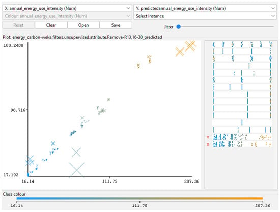
Figure 3. Predicted versus actual EUI for RF model. Generated using RF regressions analysis in Weka. Adapted from the author’s dissertation [37].

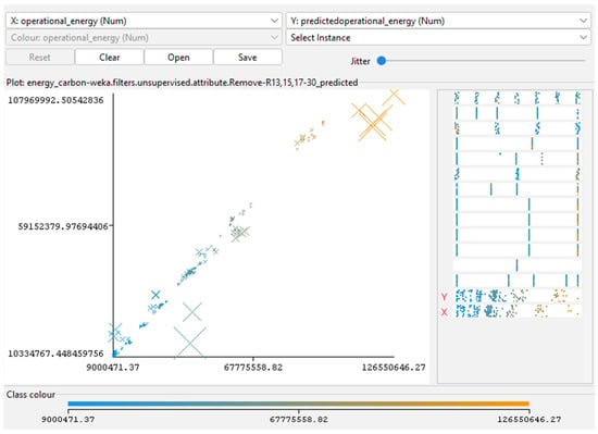
Figure 4. Predicted versus actual OE for RF model. Generated using RF regressions analysis in Weka. Adapted from the author’s dissertation [37].

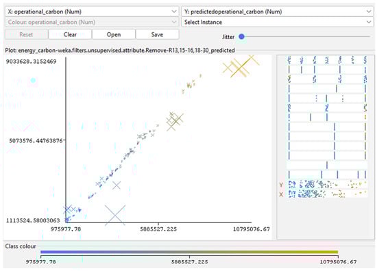
Figure 5. Predicted versus actual OC for RF model. Generated using RF regressions analysis in Weka. Adapted from the author’s dissertation [37].

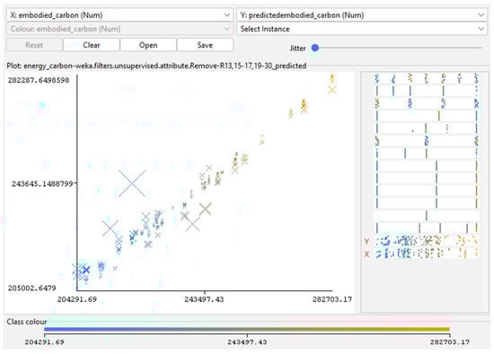
Figure 6. Predicted versus actual EC for RF model. Generated using RF regressions analysis in Weka. Adapted from the author’s dissertation [37].

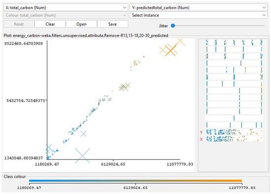
Figure 7. Predicted versus actual EUI for RF model. Generated using RF regressions analysis in Weka. Adapted from the author’s dissertation [37].

3.2. Feature Importance and Parameter Influence

Feature-importance analysis was carried out using ClassifierAttributeEval with the Ranker method, applying RF as the evaluation model. This process quantified how strongly each independent variable contributed to predicting energy and carbon outcomes.

Across all indicators, the results showed that HVAC system type, glazing ratios (WWR), and operation schedule had the greatest influence. These parameters directly affect heating and cooling loads, internal gains, and equipment operation, which explains their dominant role in both energy use and carbon emissions. LPD and infiltration rate followed as secondary drivers, reflecting their impact on internal loads and envelope performance.

Geometric factors, such as shape and orientation, had lower relative importance, but they still influenced results through interactions related to façade exposure, solar gains, and surface-area-to-volume ratios.

For carbon-related outputs, HVAC system type remained the single most influential variable, as it governs both energy demand and the associated emissions intensity. Operation schedule and LPD also played stronger roles in OC prediction, while TC reflected the combined influence of operational parameters and façade glazing assumptions embedded in Insight’s baseline embodied-carbon calculations.

Table 9 and Table 10 present the normalized importance rankings for all predictors.

Table 9. Feature importance ranking for EUI and OE using RF.

Rank	Attribute	Importance Score (EUI) %	Importance Score (OE) %	Relative Category
1	HVAC system	16.4	15.2	System
2	WWR North	15.4	14.4	Envelope
3	WWR East	15.2	14.2	Envelope
4	Operation Schedule	12.9	12.4	Operational
5	WWR South	11.2	10.5	Envelope
6	WWR West	10.5	10.0	Envelope
7	Plug Loads	9.7	9.2	Operational
8	Infiltration	9.0	8.4	Envelope
9	LPD	7.3	7.0	Operational
10	Orientation	5.0	4.6	Envelope
11	Building Lifespan	0.0	0.0	Fixed
12	Building Area	−1.7	−1.6	Geometric
13	Shape	−1.9	−1.8	Geometric

Derived from BIM-ML model results in Weka. Adapted from the author’s dissertation [37].

Table 10. Feature importance ranking for OC, EC, and TC using RF for the 168 models dataset and 210 models dataset.

Rank	OC and TC Results for the 168 Models Dataset and 210 Models Dataset	EC Results for 168 Models Dataset	EC Results for 210 Models Dataset
	Attribute	Attribute	Attribute
1	Operation Schedule	WWR South	WWR South
2	Plug Loads	WWR North	WWR North
3	WWR North	WWR West	HVAC System
4	WWR East	HVAC System	WWR West
5	HVAC System	WWR East	WWR East
6	LPD	Infiltration	Infiltration
7	WWR West	Building Area	Building Area
8	WWR South	Shape	Shape
9	Infiltration	Operation Schedule	Operation Schedule
10	Orientation	Orientation	Orientation
11	Building Lifespan	LPD	LPD
12	Building Area	Plug Loads	Plug Loads
13	Shape	Building Lifespan	Building Lifespan

Derived from BIM-ML model results in Weka. Adapted from the author’s dissertation [37].

The purpose of the feature-importance ranking is to identify a relative hierarchy of design parameters rather than to quantify absolute causal effects. By ranking variables across all five performance indicators, the analysis highlights which early-stage design decisions most strongly influence energy and carbon outcomes under limited design information. Parameters consistently ranked high, such as HVAC system type, operation schedule, and glazing ratios, represent high-impact levers that designers can prioritize during conceptual design. Lower-ranked variables, including geometry and orientation, remain relevant but exert influence primarily through secondary interactions. The consistency of rankings across multiple performance metrics and dataset sizes confirms the robustness of the observed parameter influence patterns and supports their use as interpretable guidance for early-stage sustainable design decision-making.

Accordingly, the rankings are intended to support comparative decision-making rather than deterministic prediction of individual design outcomes.

3.3. Climate Sensitive Analysis

To examine how regional climate conditions influence energy-related emissions and long-term carbon performance, ten selected models from the Orlando dataset were re-simulated using weather files from five additional U.S. cities: San Francisco (3C), Minneapolis (6A), Phoenix (2B), Denver (5B), and Seattle (4C). These models were used only for comparative analysis and were not included in ML training. This approach allowed the design parameters to remain constant while isolating the effects of outdoor climate on carbon-related indicators.

The results (Table 11) show that OPCI was the most climate-sensitive metric. Hot–humid and hot–dry locations (Orlando and Phoenix) displayed the highest Operational Carbon intensities, with values more than fourteen times higher than the LEED baseline threshold (12 kgCO₂e/ft²·yr). These elevated emissions are consistent with continuous cooling and dehumidification loads in warm climates.

Table 11. Comparative analysis of simulated OPCI, ECI₂₀, TCI₂₀, and LEED threshold across climate zones.

Location	OPCI (kgCO2/ft2.yr)	ECI20 (kgCO2/yr)	TCI20 (kgCO2/ft2)	Compliance Outcome	Observation
Orlando (2A)	190.0 (+1483.0%)	8.0 (−73.3%)	198.0 (−69.5%)	No for OPCI and Yes for ECI20 and TCI20	Highest carbon intensity due to continuous cooling and dehumidification demands. HVAC system efficiency dominates OPCI results, while envelope performance has limited mitigation under hot–humid loads.
San Francisco (3C)	154.27 (+1185.6%)	8.0 (−73.3%)	162.3 (−75.4%)	No for OPCI and Yes for ECI20 and TCI20	Mild coastal climate results in moderate Operational Carbon despite limited HVAC use; internal and lighting loads maintain relatively steady emissions.
Minneapolis (6A)	152.2 (+1168.7%)	8.0 (−73.3%)	160.3 (−75.4%)	No for OPCI and Yes for ECI20 and TCI20	Cold-humid climate increases heating carbon intensity; efficient envelope design partially offsets HVAC loads, keeping Total Carbon close to mid-range values.
Phoenix (2B)	190.7 (+1489.3%)	8.0 (−73.3%)	198.7 (−69.4%)	No for OPCI and Yes for ECI20 and TCI20	Extreme cooling loads drive OPCI to the highest levels after Orlando. The dry environment limits infiltration but sustained air-conditioning use amplifies carbon intensity.
Denver (5B)	156.5 (+1204.4%)	8.0 (−73.3%)	164.6 (−74.7%)	No for OPCI and Yes for ECI20 and TCI20	Mixed–dry climate yields balanced heating and cooling impacts. Moderate elevation lowers cooling demand slightly, stabilizing carbon performance near mid-range.
Seattle (6A)	127.1 (+959.0%)	8.0 (−73.3%)	134.9 (−79.2%)	No for OPCI and Yes for ECI20 and TCI20	Marine climate produces the lowest OPCI and TCI20 among all cities due to mild seasonal variation and minimal HVAC reliance, though still above LEED baseline limits.

Based on simulated results from Autodesk Insight (2024) and LEED v4 baseline thresholds [41]. Adapted from the author’s dissertation [37].

Cities with colder (Minneapolis) or marine (Seattle) climates recorded noticeably lower OPCI values but still exceeded LEED’s target. Seattle achieved the lowest TCI₂₀ among all locations due to mild temperatures and limited HVAC demand throughout the year. Denver and Minneapolis presented mid-range results, driven by a balance between heating requirements and reduced cooling loads.

As expected, ECI₂₀ remained unchanged across all cities. Because EC depends solely on material quantities and construction assumptions, it is unaffected by climatic variations.

Overall, the cross-climate analysis indicates that

• climate strongly affects operational and TC performance;
• EC is climate-independent; and
• proportional relationships among OPCI, ECI₂₀, and TCI₂₀ remain consistent.

This confirms that the simulation framework generates stable carbon-performance patterns across regions while still reflecting the expected influence of climate on operational emissions.

3.4. Case Study Validation Results

Two LEED Gold-certified buildings on the University of Central Florida (UCF) main campus—UCF Global and UCF Research I—were used to evaluate how well the surrogate model performs when applied to real buildings. Both facilities are three-story office-type structures located in Orlando, Florida (Climate Zone 2A), which aligns with the climate used for the main simulation dataset. Although similar in height and general use, the buildings differ in size and internal load patterns, providing two distinct validation conditions.

Table 12 summarizes their key characteristics, including building function, GFA, operational schedule, and LEED certification level.

Table 12. Validation building characteristics.

Building	Function	Area (ft2)	Floors	Schedule	LEED Version
UCF Global	Administrative	52,766	3	8 a.m.–5 p.m.	v3
UCF Research I	Academic	111,000	3	8 a.m.–5 p.m.	v3

Based on building documentation and LEED certification records from the University of Central Florida Utilities and Engineering Services (personal communication, 2025). Adapted from the author’s dissertation [37].

Measured electricity consumption for 2023 and 2024 was obtained from UCF Utilities and Engineering Services and matched with the LEED performance documentation. OC for each building was calculated using the regional emission factor for the Southeast eGRID subregion (0.331 kgCO₂e/kWh). Both buildings showed small year-to-year reductions in EUI and OC, consistent with stable operating patterns and incremental efficiency improvements. These measured values are presented in Table 13 and Table 14.

Table 13. Measured performance data—UCF Global building.

Year	Annual Electricity (kWh)	EUI (kBtu/ft2·yr)	OC (kg CO2)	Grid Factor	Floors
2023	503,200	32.50	166,560	0.331	3
2024	470,443	30.40	155,717	0.331	3

Based on building documentation and LEED certification records from the University of Central Florida Utilities and Engineering Services (personal communication, 2025). Adapted from the author’s dissertation [37].

Table 14. Measured performance data—UCF Research I building.

Year	Annual Electricity (kWh)	EUI (kBtu/ft2·yr)	OC (kg CO2)	Grid Factor	Floors
2023	1,593,071	73.00	527,307	0.331	3
2024	1,497,981	68.60	495,832	0.331	3

Based on building documentation and LEED certification records from the University of Central Florida Utilities and Engineering Services (personal communication, 2025). Adapted from the author’s dissertation [37].

The Random Forest (RF) model was then used to predict EUI and OC under three schedule scenarios—standard office hours (8–5), extended hours (12/5), and continuous operation (24/7). This allowed assessment of how the surrogate model responds to different occupancy assumptions. Predicted and observed values are shown in Table 15.

Table 15. Predicted versus measured EUI and OC for UCF buildings.

Building	Operation Schedule	Measured EUI—2023 (kBtu/ft2·yr)	Measured EUI—2024 (kBtu/ft2·yr)	Predicted EUI (kBtu/ft2·yr)	Measured OC—2023 (kgCO2e)	Measured OC—2024 (kgCO2e)	Predicted OC (kgCO2e)
UCF Global (8–5)	Office hours	32.50	30.40	65.24	166,560	155,717	4,056,509
UCF Global (12/5)	Extended	32.50	30.40	58.28	166,560	155,717	3,597,330
UCF Global (24/7)	Continuous	32.50	30.40	71.36	166,560	155,717	4,784,152
UCF Research I (8–5)	Office hours	73.00	68.60	70.32	527,307	495,832	3,657,026

Derived from BIM-ML model results in Weka and based on building documentation and LEED certification records from the University of Central Florida Utilities and Engineering Services (personal communication, 2025). Adapted from the author’s dissertation [37]. Predicted OC values are based on default simulation carbon-intensity factors and are not calibrated to UCF-specific electricity emission coefficients.

Overall, the RF model reproduced energy relative energy-performance trends reasonably well, particularly in capturing the ranking between case-study buildings, while absolute agreement varied depending on building-specific operational characteristics. For UCF Global, predicted EUI under the 8–5 schedule was higher with measured values, while the 12/5 and 24/7 scenarios showed the expected directional increases in energy use associated with longer operation. For UCF Research I, the predicted EUI also closely matched observed performance, indicating that the model generalizes effectively across two different office-type buildings within the same climate zone.

In contrast, OC predictions were consistently much higher than measured values, often by an order of magnitude. This discrepancy reflects the use of Insight’s default national-average carbon intensity during simulation, whereas the measured OC values are based on UCF-specific electricity procurement and Florida regional grid emission factors. Because OC is directly tied to emission coefficients rather than energy demand alone, the surrogate model inevitably reproduced this overestimation.

These results highlight three key findings:

• energy predictions generalized well across building sizes, functions, and schedule assumptions;
• carbon predictions were systematically inflated, not due to model error, but because the underlying simulations used non-localized emission factors; and
• regional carbon-factor adjustments are necessary to obtain realistic OC and TC estimates for Florida-based buildings.

This stage of the analysis therefore confirmed that the surrogate model is reliable for predicting energy use but requires region-specific emission inputs to achieve accurate operational-carbon predictions, an issue addressed in the carbon-factor correction described in the next section.

Carbon Factor Correction

The validation results showed that the carbon estimates produced by Insight were consistently higher than the measured values for the two UCF buildings. This discrepancy occurred because Insight applies a generic U.S. average grid emission factor (0.45 kg CO₂e/kWh), which is considerably higher than the carbon intensity of Florida’s electricity mix. To correct for this mismatch, Operational Carbon values were recalculated using the region-specific emission factor from EPA eGRID (2024) for the Florida Reliability Coordinating Council (FRCC) subregion: 0.331 kg CO₂e/kWh (see Table 16).

Table 16. Regional carbon factor adjustments for UCF buildings.

UCF Global Building
Operation Schedule	Carbon Factor Correction	Operational Carbon (kgCO2e)	TCI20 (kgCO2e/ft2)
8 a.m.–5 p.m.	Before correction	4,056,508.6	138.21
12/5		3,597,329.7	120.89
24/7		4,784,152.1	165.85
8 a.m.–5 p.m.	After correction	3,784,617.2	133.83
12/5		3,476,174.6	117.83
24/7		4,174,562.2	142.75
UCF Research I Building
Operation Schedule	Carbon Factor Correction	Operational Carbon (kgCO2e)	TCI20 (kgCO2e/ft2)
8 a.m.–5 p.m.	Before correction	3,657,026.0	125.32
	After correction	4,096,039.8	145.41

Derived from BIM-ML model results in Weka and based on building documentation and LEED certification records from the University of Central Florida Utilities and Engineering Services (personal communication, 2025). Adapted from the author’s dissertation [37].

This adjustment was applied only to OC and TCI₂₀ because both indicators are directly tied to electricity-related emissions. EUI and OE were unchanged, as they represent energy use rather than carbon output, and EC is unrelated to grid electricity.

After recalculating OC and TCI₂₀ with the Florida-specific factor, the ML models were retrained to reflect the corrected carbon baseline. The updated models showed notably better agreement with the measured data, indicating that the regional adjustment improved the realism of the carbon predictions. The correction also reduced the spread between operational schedule scenarios, producing more stable TCI₂₀ differences for UCF Global and yielding values for UCF Research I that better matched expected local conditions.

Overall, applying the regional emission factor increased consistency across building types, strengthened the calibration of the surrogate model, and aligned the analysis with the carbon-accounting method used in UCF’s LEED reporting practices. This step ensures that the BIM-ML framework provides carbon predictions that are reflective of the electricity grid where the buildings operate.

4. Discussion

The BIM-ML framework developed in this study performed well across all prediction tasks, showing that ML surrogates can support early design evaluations of office buildings. Among the tested algorithms, the RF model delivered the most accurate and stable results for both energy and carbon metrics, consistently achieving high R² values and low error rates. These outcomes indicate that the surrogate effectively captured nonlinear interactions among geometry, systems, and operational parameters while remaining computationally efficient.

Feature-importance results offered further insight into which parameters most influenced performance. HVAC system choice emerged as the strongest predictor of energy outcomes, followed by glazing ratios on key façades and operation schedule. These findings are consistent with established building-physics principles, especially in hot–humid climates where cooling loads dominate. For carbon indicators, HVAC system efficiency and internal load assumptions (LPD and plug loads) played central roles in shaping operational emissions, whereas EC was influenced more by geometric characteristics and façade configuration.

Climate-sensitivity tests showed that while absolute energy and carbon levels shifted across locations, reflecting differences in heating and cooling loads, the relative performance of the modeled design options remained stable. Designs that performed well in the Orlando baseline largely retained their ranking in milder or colder climates. This suggests that the surrogate captures consistent performance patterns even when applied outside its training climate, reinforcing its usefulness for early comparative evaluations.

Validation with two LEED-certified UCF buildings further tested real-world applicability. The RF model closely matched measured EUI values, with deviations within ±5%. However, OC predictions were initially overestimated due to the use of Insight’s national average carbon factor. Once emissions were recalculated using the Florida-specific eGRID factor, the surrogate’s carbon predictions aligned more closely with measured values. This highlights that accurate carbon assessment depends not only on energy-prediction quality but also on applying region-specific emission coefficients.

Overall, the results show that the RF-based BIM-ML framework provides a practical and accurate method for early performance assessment. Energy predictions remain robust across climates and validation cases, while carbon predictions improved substantially when paired with localized emission data. These findings emphasize the value of ML surrogates in early design while also identifying key methodological considerations for reliable carbon evaluation.

4.1. Methodological Contributions

The study contributes a structured methodology that combines DOE principles with BIM-based simulations to generate a balanced and statistically meaningful dataset. The reduced-factorial DOE ensured broad coverage of parameter interactions while keeping the simulation workload manageable. This approach supports transparency, reproducibility, and efficient exploration of the early-design space.

The workflow linking Revit, Insight, and Weka demonstrates that high-quality training data and ML analysis can be produced using standard design and simulation tools without custom coding. Insight provided consistent energy and carbon outputs grounded in ASHRAE 90.1 Appendix G assumptions, while Weka offered accessible model-building and feature-importance analysis. Together, these tools create a repeatable pipeline that can be adapted to other climates or building types.

4.2. Implications for Design Practice and Sustainability Evaluation

For design teams, the proposed framework offers a fast and practical way to test multiple design options early in the process, when changes are easiest and most impactful. Once trained, the ML surrogate can estimate performance in seconds, allowing quick exploration of alternative geometries, system choices, and operational scenarios.

By linking predictions directly to BIM data, the approach supports early benchmarking against LEED and carbon-reduction targets and enables designers to understand how decisions about HVAC systems, glazing, loads, and schedules translate into energy and carbon impacts. Because the workflow is based on commonly used Autodesk software (Autodesk Revit 2024 and Autodesk Insight Carbon Analysis 2023.1) and open-source ML tools (Weka v3.8.6), it can be integrated into existing design practices and extended to region-specific or institution-wide applications.

4.3. Limitations and Future Work

Although the framework performed well, several limitations must be acknowledged. First, EC results relied on Insight’s default material assumptions, which provide generalized emission factors rather than product-specific values. This limits the precision of EC comparisons, especially for studies involving detailed material substitutions or advanced façade systems.

Second, OC validation was based on only two real buildings. While the regional carbon-factor adjustment improved accuracy, a broader validation set is needed to confirm generalizability across different building sizes, systems, and operational patterns.

Third, the dataset was intentionally limited to mid-rise office prototypes to maintain geometric consistency. This strengthens internal validity but limits the applicability of the trained models to other building types. Future work should test the framework on residential, educational, or high-rise buildings with different occupancy and load profiles.

Based on these limitations, future studies should consider the following:

• using detailed LCA databases (e.g., EC3, OneClick LCA, and regional EPDs) for more accurate EC estimates;
• exploring more advanced ML models, such as deep neural networks or ensemble hybrids, to capture complex nonlinear patterns in larger datasets;
• automating dataset generation using Dynamo or the Revit API to scale up the number of simulations and expand parameter diversity; and
• embedding real-time ML dashboards in Revit to provide instant feedback on energy and carbon performance during modeling.

5. Conclusions

This study demonstrates that integrating BIM-based simulations with ML provides an effective approach for predicting early-stage building energy and carbon performance. Using a reduced-factorial dataset and standard parametric simulation tools, the RF surrogate achieved high predictive accuracy for both energy (EUI and OE) and carbon (OC, EC, and TC) metrics, with R² values exceeding 0.97. These results indicate that ML models can reliably approximate Insight outputs while requiring only a fraction of the computational effort.

Feature-importance analysis showed that HVAC system type, glazing ratio, and operation schedule were the dominant drivers of predicted performance, reflecting well-established sensitivity in warm–humid climates. Geometric variables contributed less directly but remained relevant through their influence on envelope exposure and gains.

Climate sensitivity tests confirmed that although absolute performance changed across locations, the relative ranking of design alternatives remained consistent. Validation using two LEED-certified office buildings further demonstrated strong agreement for energy use, while carbon estimates required the application of region-specific emission factors. Adjusting OC and TC using EPA eGRID values improved alignment with measured data and highlighted the importance of localized carbon-intensity coefficients when applying surrogate models in practice.

Overall, the findings indicate that the proposed BIM-ML workflow is a practical and transferable method for early-stage sustainability assessment. The framework is transparent, reproducible, and compatible with common design tools, enabling rapid evaluation of multiple design scenarios and supporting early decision-making aligned with energy-efficiency and carbon-reduction goals.

Building on these findings, future research will focus on expanding the framework beyond office buildings, incorporating higher-resolution regional emissions data, and strengthening typological validation across diverse building programs. Additional work may also explore tighter integration of BIM-ML surrogate models within early design workflows to support interactive sustainability decision-making.

While this study evaluated representative ASHRAE climate zones to test model adaptability, extending the framework to all 19 ASHRAE climate zones is identified as an important direction for future research. Such expansion would further strengthen nationwide applicability and support climate-specific calibration of BIM-ML surrogate models.

In addition, incorporating higher-resolution EC data and expanding validation across additional building typologies would further enhance the applicability of ML-based surrogates within performance-driven design processes.

References

- Ritchie, H.; Rosado, P. Energy Mix. Our World in Data. January 2024. Available online: https://ourworldindata.org/energy-mix (accessed on 20 October 2025).
- Seyedzadeh, S.; Ramezani, P.F.; Glesk, I.; Roper, M. Machine learning for estimation of building energy consumption and performance: A review. Vis. Eng. 2018, 6, 5. [Google Scholar] [CrossRef]
- Ahmad, A.S.; Hassan, M.Y.; Abdullah, H.; Rahman, H.A.; Hussin, F.; Abdullah, M.P.; Said, D.M. A review on applications of ANN and SVM for building electrical energy consumption forecasting. Renew. Sustain. Energy Rev. 2018, 33, 102–109. [Google Scholar] [CrossRef]
- Kalogirou, S.A. Applications of artificial neural networks in energy systems: A review. Energy Convers. Manag. 1999, 40, 1073–1087. [Google Scholar]
- Duarte, G.R.; Fonseca, L.G.; Goliatt, P.V.Z.C.; Lemonge, A.C.C. Comparison of machine learning techniques for predicting energy loads in buildings. Ambient. Constr. 2017, 17, 3. [Google Scholar]
- Fumo, N.; Biswas, M.A.R. Regression analysis for prediction of residential energy consumption. Renew. Sustain. Energy Rev. 2015, 47, 332–343. [Google Scholar] [CrossRef]
- Seyedzadeh, S.; Rahimian, F.P.; Rastogi, P.; Glesk, I. Tuning machine learning models for prediction of building energy loads. Sustain. Cities Soc. 2019, 47, 101484. [Google Scholar] [CrossRef]
- Manfren, M.; Nastasi, B.; Tronchin, L. Data-driven building energy modelling: Analytical and practical challenges. Renew. Sustain. Energy Rev. 2022, 160, 112253. [Google Scholar]
- Miller, C.; Picchetti, B.; Fu, C.; Pantelic, J. Limitations of machine learning for building energy prediction: Error analysis from the ASHRAE Great Energy Predictor III competition. Sci. Technol. Built Environ. 2022, 28, 610–627. [Google Scholar] [CrossRef]
- U.S. Green Building Council (USGBC). How LEED v4.1 Addresses Embodied Carbon; U.S. Green Building Council: Washington, DC, USA, 2021; Available online: https://www.usgbc.org/articles/how-leed-v41-addresses-embodied-carbon (accessed on 20 October 2025).
- Fenton, S.K.; Munteanu, A.; De Rycke, K.; De Laet, L. Embodied greenhouse gas emissions of buildings—A machine learning approach for early-stage prediction. Build. Environ. 2024, 257, 111523. [Google Scholar] [CrossRef]
- Xie, Q.; Jiang, Q.; Kurnitski, J.; Yang, J.; Lin, Z.; Ye, S. Quantitative carbon emission prediction model for embodied carbon in multi-story buildings. Sustainability 2024, 16, 5575. [Google Scholar] [CrossRef]
- Cang, Y.; Luo, Z.; Yang, L.; Wang, W.; Si, Q.; Zhang, J.; Tong, Y. Prediction method of building embodied carbon emissions for conceptual design using machine learning. Build. Environ. 2026, 289, 114053. [Google Scholar]
- Nwodo, M.; Anumba, C.J. Exergy-Based Life Cycle Assessment of Buildings: Case Studies. Sustainability 2021, 13, 11682. [Google Scholar] [CrossRef]
- Hong, T.; Luo, X.; Zhang, W. Ten questions on data-driven building performance modeling. Build. Environ. 2020, 168, 106508. [Google Scholar] [CrossRef]
- Feng, K.; Lu, W.; Wang, Y. Assessing environmental performance in early building design stage: An integrated parametric design and machine learning method. Sustain. Cities Soc. 2019, 50, 101596. [Google Scholar] [CrossRef]
- Zhang, G.; Sandanayake, M. BIM and optimisation techniques to improve sustainability in green certification submission of construction projects. In Proceedings of the 7th World Construction Symposium (WCS 2018), Colombo, Sri Lanka, 29 June–1 July 2018. [Google Scholar]
- Gan, V.J.L.; Lo, I.M.C.; Ma, J.; Tse, K.T.; Cheng, J.C.P.; Chan, C.M. Simulation optimisation towards energy efficient green buildings: Current status and future trends. J. Clean. Prod. 2020, 254, 120012. [Google Scholar] [CrossRef]
- Pan, X.; Khan, A.M.; Eldin, S.M.; Aslam, F.; Rehman, S.K.U.; Jameel, M. BIM adoption in sustainability, energy modelling and implementing using ISO 19650: A review. Ain Shams Eng. J. 2024, 15, 102252. [Google Scholar] [CrossRef]
- Singh, M.M.; Deb, C.; Geyer, P. Early-stage design support combining machine learning and BIM. Autom. Constr. 2022, 136, 104147. [Google Scholar] [CrossRef]
- Robinson, C.; Dilkina, B.; Hubbs, J.; Zhang, W.; Guhathakurta, S.; Brown, M.A.; Pendyala, R.M. Machine learning approaches for estimating commercial building energy consumption. Appl. Energy 2017, 208, 889–904. [Google Scholar] [CrossRef]
- Geyer, P.; Singaravel, S. Component-based machine learning for performance prediction in building design. Appl. Energy 2018, 228, 1439–1453. [Google Scholar] [CrossRef]
- Ali, A.; Jayaraman, R.; Jayaraman, A.; Jayaraman, B.; Azar, E. Machine learning as a surrogate to building performance simulation: Predicting energy consumption under different operational settings. Energy Build. 2023, 286, 112940. [Google Scholar] [CrossRef]
- Kim, J.; Jung, J.H.; Kim, S.J.; Kim, S.A. Multi-factor optimization method through machine learning in building envelope design: Focusing on perforated metal façade. Int. J. Archit. Environ. Eng. 2017, 11, 1–8. [Google Scholar]
- Rahmani Asl, M.; Xu, W.; Shang, J.; Tsai, B.; Molloy, I. Regression-Based Building Energy Performance Assessment Using Building Information Model (BIM). In Proceedings of the ASHRAE and IBPSA-USA SimBuild 2016 Building Performance Modeling Conference, Salt Lake City, UT, USA, 8–12 August 2016; pp. 1–8. [Google Scholar]
- Chen, Z.; Xiao, F.; Guo, F.; Yan, J. Interpretable machine learning for building energy management. Adv. Appl. Energy 2023, 9, 100123. [Google Scholar] [CrossRef]
- D’Amico, B.; Myers, R.J.; Sykes, J.; Voss, E.; Cousins-Jenvey, B.; Fawcett, W.; Richardson, S.; Kermani, A.; Pomponi, F. Machine learning for sustainable structures: A call for data. Structures 2019, 19, 1–4. [Google Scholar] [CrossRef]
- Ma, G.; Liu, Y.; Shang, S. A building information model (BIM) and artificial neural network (ANN) based system for personal thermal comfort evaluation and energy efficient design of interior space. Sustainability 2019, 11, 4972. [Google Scholar] [CrossRef]
- Hollberg, A.; Genova, G.; Habert, G. Evaluation of BIM-based LCA results for building design. Autom. Constr. 2020, 109, 102972. [Google Scholar] [CrossRef]
- Khan, A.A.; Khan, M.A.; Ahmad, N.; Jamil, F.; Imran, M.; Abaker, M. Integrating Building Information Modelling and artificial intelligence: A systematic review of challenges and mitigation strategies. Technologies 2024, 12, 185. [Google Scholar] [CrossRef]
- Meng, G.; Zhang, L.; Huang, Y.; Wu, Z. The application obstacles of BIM technology in green building projects. Sci. Rep. 2024, 14, 18839. [Google Scholar] [CrossRef] [PubMed]
- Ning, C.; You, F. Optimization under uncertainty in the era of big data and deep learning: When machine learning meets mathematical programming. Comput. Chem. Eng. 2019, 125, 434–448. [Google Scholar] [CrossRef]
- Walker, S.; Khan, W.; Katic, K.; Maassen, W.; Zeiler, W. Accuracy of different machine learning algorithms and added-value of predicting aggregated-level energy performance of commercial buildings. Energy Build. 2020, 209, 109705. [Google Scholar] [CrossRef]
- Kim, Y.M.; Ahn, K.U.; Park, C.S. Issues of application of machine learning models for virtual and real-life buildings. Sustainability 2016, 8, 543. [Google Scholar] [CrossRef]
- Box, G.E.P.; Hunter, J.S.; Hunter, W.G. Statistics for Experimenters: Design, Innovation, and Discovery, 2nd ed.; John Wiley & Sons: Hoboken, NJ, USA, 2005. [Google Scholar]
- Montgomery, D.C. Design and Analysis of Experiments, 9th ed.; John Wiley & Sons: Hoboken, NJ, USA, 2017. [Google Scholar]
- Magnavaca de Paula, L. BIM-Based Machine Learning Surrogate Models for Energy and Carbon Prediction to Support LEED Certification Evaluation. Doctoral Dissertation, University of Central Florida, Orlando, FL, USA, 2025. [Google Scholar]
- ANSI/ASHRAE/IES Standard 90.1-2019; Energy Standard for Buildings Except Low-Rise Residential Buildings. American Society of Heating, Refrigerating and Air-Conditioning Engineers: Atlanta, GA, USA, 2019.
- U.S. Energy Information Administration (EIA). Electricity Explained. 2023. Available online: https://www.eia.gov/energyexplained/electricity/electricity-in-the-us.php (accessed on 20 October 2025).
- U.S. Department of Energy (DOE). Energyplus: Building Energy Simulation Program. Available online: https://energyplus.net (accessed on 20 October 2025).
- U.S. Green Building Council. Materials & Resources category: Building Life-Cycle Impact Reduction. In LEED v4 Reference Guide for Building Design + Construction; U.S. Green Building Council: Washington, DC, USA, 2020. [Google Scholar]
- ANSI/ASHRAE Standard 169-2013; Climatic Data for Building Design Standards. American Society of Heating, Refrigerating and Air-Conditioning Engineers (ASHRAE): Atlanta, GA, USA, 2013.
Disclaimer/Publisher’s Note: The statements, opinions and data contained in all publications are solely those of the individual author(s) and contributor(s) and not of MDPI and/or the editor(s). MDPI and/or the editor(s) disclaim responsibility for any injury to people or property resulting from any ideas, methods, instructions or products referred to in the content. |
© 2026 by the authors. Licensee MDPI, Basel, Switzerland. This article is an open access article distributed under the terms and conditions of the Creative Commons Attribution (CC BY) license.