Bipartite Synchronization for Signed Luré Networks via Semi-Markovian Jump Switching and Quantized Pinning Control

Abstract

This paper investigates bipartite synchronization in signed Lur’e networks influenced by semi-Markovian jump dynamics. A control strategy is proposed that adapts to mode-dependent switching by combining quantized feedback with selective pinning. The approach accommodates both leaderless and leader–following synchronization scenarios. For each switching mode, Lyapunov–Krasovskii-based analysis is employed to establish sufficient conditions using linear matrix inequalities (LMIs). The robustness and convergence of the method are confirmed through simulation studies, even in the presence of stochastic switching and limited communication precision.

1. Introduction

Synchronization phenomena in complex networks (CNs) play a vital role across various applications, including distributed sensing, cooperative control, and signal processing. Within this broad context, bipartite synchronization has drawn considerable interest, particularly in networks characterized by both cooperative and antagonistic interactions. These interactions are efficiently modeled through signed graphs, which incorporate structural features such as sign symmetry and structural balance to describe system dynamics accurately [1,2,3]. Depending on the nature of coordination among nodes, synchronization strategies are generally classified into leaderless and leader–following categories. Although leader–following methods introduce external driving signals to guide synchronization, they often incur increased communication and control overhead. To address these challenges, pinning control has been proposed as a cost-effective technique, achieving synchronization by selectively controlling a subset of network nodes [4,5,6,7,8].

Significant progress has been made in understanding bipartite synchronization within signed networks. For instance, Ai et al. proposed a multi-leader synchronization scheme [9], while Zhang et al. analyzed continuous-time dynamics over signed graphs [10]. Other works such as [11,12] employed Laplacian-based models to address consensus problems. However, a common limitation among these studies is the assumption of static or deterministic network structures [13], which does not fully capture the complexities of real-world systems where randomness, uncertainties, and dynamic topology switching are prevalent [14].

It is also worth noting that, in practical cyber–physical networks, limited communication precision may coexist with component faults or partial loss of actuation. This has motivated fault-tolerant synchronization/formation/consensus designs for networked multi-agent systems under switching topologies (see, e.g., [15] and related works). In parallel, performance-driven (optimization-oriented) fault-tolerant control for switched systems has been studied to preserve stability and regulation quality under actuator degradations and constraints. For Markov jump models, fuzzy tracking in the presence of mismatched faults has also been investigated using observer-based schemes such as iterative proportional–integral designs [16]. These results are closely related in motivation; however, they do not address bipartite synchronization for signed Lur’e networks under semi-Markov switching with the quantized pinning structure considered here.

To bridge this gap, this paper introduces a semi-Markovian jump system (SMJS) framework for analyzing bipartite synchronization in signed Lur’e networks. Unlike conventional Markov jump models, SMJSs allow for arbitrary sojourn time distributions, offering a more flexible and realistic representation of switching behaviors in dynamic networks.

Lur’e-type systems are particularly well-suited for this study due to their general nonlinear feedback configurations and their wide-ranging applications, including encryption, aerospace engineering, and hydraulic control systems [17,18,19,20]. Building upon the foundation established by recent research on quantized bipartite control [21,22], this work extends existing models by incorporating Semi-Markovian switching mechanisms, quantization effects, and pinning strategies into the control design.

Inspired by [21,23,24], the main contributions of this paper are summarized as follows:

• A novel semi-Markovian jump framework is proposed for achieving bipartite synchronization in signed Lur’e networks, considering stochastic switching governed by arbitrary sojourn times.
• A quantized bipartite control scheme is designed for both leaderless and leader–following synchronization settings, and sufficient stability conditions are established through Lyapunov–Krasovskii functionals and mode-dependent LMI formulations.
• Extensive numerical simulations are conducted to verify the theoretical results, demonstrating the convergence and robustness of the proposed control approach under stochastic switching and limited communication.

The remainder of the paper is organized as follows: Section 2 reviews relevant graph-theoretic concepts and stochastic system preliminaries. Section 3 formulates the bipartite synchronization problem. Section 4 presents the main theoretical results. Section 5 illustrates simulation results, and Section 6 concludes the study.

Notation

In this paper, $\parallel ·\parallel$ denotes the standard Euclidean norm in a vector space. For any matrix A, ${\lambda }_{max}\left(A\right)$ and ${\lambda }_{min}\left(A\right)$ represent the largest and smallest eigenvalues of A, respectively. The set of real numbers is denoted by $\mathbb{R}$, and ${\mathbb{R}}^n$ refers to the n-dimensional Euclidean space. The index set of nodes in the network is denoted by ${\partial }_N=\{1,2,\dots ,N\}$. The N-dimensional identity matrix is written as $I_N$, while the Kronecker product between matrices is represented by the symbol ⊗.

The semi-Markov process, denoted by $\sigma \left(t\right)$, is modeled as a piecewise constant stochastic process taking values in a finite set $\mathcal{S}=\{1,2,\dots ,r\}$. Its dynamics are characterized by a transition probability matrix $Q=\left[q_{ij}\right]$ and mode-specific sojourn time distribution functions $F_{ij}\left(t\right)$. The indicator function ${⊮}_{\{·\}}$ returns 1 if the condition inside the brackets is satisfied and 0 otherwise.

For any matrix $D\in {\mathbb{R}}^{n\times n}$, its symmetric part is defined as $D_s={\displaystyle \frac{1}{2}}(D+D^T)$. A block matrix of the form

$$\left(\begin{array}{cc}A& B\\ B^T& C\end{array}\right)$$

is considered symmetric if A and C are symmetric matrices and $B^T$ denotes the transpose of B.

2. Preliminaries

Consider a signed directed graph $\mathcal{G}=(\mathcal{U},\mathcal{V},\mathcal{A})$, where $\mathcal{U}$ denotes the set of nodes, $\mathcal{V}$ represents the set of edges, and $\mathcal{A}=\left[a_{ik}\right]$ is the corresponding signed adjacency matrix. The presence of an edge from node i to node k is indicated by a nonzero element $a_{ik}$. The Laplacian matrix associated with $\mathcal{G}$ is given by $\mathcal{L}=C-\mathcal{A}$, where C is a diagonal matrix with entries $c_i={\sum }_{k\ne i}\left|a_{ik}\right|$.

The graph $\mathcal{G}$ is said to be structurally balanced if the node set $\mathcal{U}$ can be partitioned into two non-overlapping subsets, ${\mathcal{U}}_1$ and ${\mathcal{U}}_2$, satisfying:

• Intra-group connections are non-negative: $a_{ik}\ge 0$ if $i,k\in {\mathcal{U}}_1$ or $i,k\in {\mathcal{U}}_2$,
• Inter-group connections are non-positive: $a_{ik}\le 0$ if $i\in {\mathcal{U}}_1$ and $k\in {\mathcal{U}}_2$ (and vice versa).

Lemma 1

(Structural Balance Transformation). If the graph $\mathcal{G}$ is structurally balanced, there exists a diagonal matrix $\mathrm{\Gamma }=\mathrm{diag}({\gamma }_1,{\gamma }_2,\dots ,{\gamma }_N)$, where each ${\gamma }_i\in \{1,-1\}$, such that:

$$\mathrm{\Gamma }\mathcal{A}\mathrm{\Gamma }=\overline{\mathcal{A}},$$

where $\overline{\mathcal{A}}$ is a matrix whose entries are the absolute values of $a_{ik}$, i.e., $\overline{\mathcal{A}}=\left(\right|a_{ik}{\left|\right)}_{N\times N}$ . This transformation effectively converts the signed graph into an unsigned one.

Lemma 2

([25]). The positive definiteness of a block matrix

$$\left(\begin{array}{cc}Q\left(x\right)& S\left(x\right)\\ S^{\top }\left(x\right)& R\left(x\right)\end{array}\right)$$

is equivalent to either of the following Schur complement conditions:

• $Q\left(x\right)>0$ and $R\left(x\right)-S^{\top }\left(x\right)Q^{-1}\left(x\right)S\left(x\right)>0$,
• $R\left(x\right)>0$ and $Q\left(x\right)-S\left(x\right)R^{-1}\left(x\right)S^{\top }\left(x\right)>0$.

3. Problem Formulation

We consider a network consisting of N identical agents, indexed by the set

$$\mathcal{N}:=\{1,2,\dots ,N\},$$

where each node evolves under a nonlinear Lur’e-type dynamic influenced by stochastic switching governed by a semi-Markov process. The dynamics of each node $i\in \mathcal{N}$ are expressed as:

$${\dot{x}}_i\left(t\right)=A_{\sigma \left(t\right)}{x}_i\left(t\right)+B_{\sigma \left(t\right)}g\left(D_{\sigma \left(t\right)}{x}_i\left(t\right)\right)+u_i\left(t\right),$$

(1)

where $x_i\left(t\right)\in {\mathbb{R}}^n$ is the state vector of node i, $u_i\left(t\right)$ represents the control input, and $\sigma \left(t\right)\in \mathcal{S}=\{1,2,\dots ,r\}$ is a semi-Markov process indicating the current operational mode.

Here, $\sigma \left(t\right)\in \mathcal{S}=\{1,\dots ,r\}$ is the semi-Markov mode at time t. For each mode $s\in \mathcal{S}$, $A_s\in {\mathbb{R}}^{n\times n}$, $B_s\in {\mathbb{R}}^{n\times m}$, and $D_s\in {\mathbb{R}}^{m\times n}$ are constant system matrices; the shorthand $A_{\sigma \left(t\right)}$, $B_{\sigma \left(t\right)}$, and $D_{\sigma \left(t\right)}$ means $A_{\sigma \left(t\right)}=A_s$, $B_{\sigma \left(t\right)}=B_s$, and $D_{\sigma \left(t\right)}=D_s$ whenever $\sigma \left(t\right)=s$.

Each switching mode $s\in \mathcal{S}$ corresponds to a unique set of system matrices $A_s$, $B_s$, and $D_s$. The nonlinear function $g(·)$ satisfies certain regularity and boundedness conditions as discussed later. The evolution of the semi-Markov process $\sigma \left(t\right)$ follows the properties:

• Initial distribution: $Pr(\sigma \left(0\right)=i)={\pi }_i$ for each $i\in \mathcal{S}$;
• Mode transition: $Pr(\sigma (t+\Delta t)=j\mid \sigma \left(t\right)=i)=q_{ij}\Delta t+o(\Delta t)$;
• Sojourn times are distributed as $F_{ij}\left(t\right)$ for transitions $i\ne j$.

In addition, a leader node is included, governed by similar mode-dependent dynamics:

$$\dot{y}\left(t\right)=A_{\sigma \left(t\right)}y\left(t\right)+B_{\sigma \left(t\right)}g\left(D_{\sigma \left(t\right)}y\left(t\right)\right),$$

(2)

where $y\left(t\right)\in {\mathbb{R}}^n$ denotes the state of the leader.

Assumption 1.

The interaction topology of the network is represented by a signed graph $\mathcal{G}$ that is structurally balanced. That is, the node set $\mathcal{U}$ can be partitioned into two disjoint subsets ${\mathcal{U}}_1$ and ${\mathcal{U}}_2$ such that intra-group edges are non-negative and inter-group edges are non-positive.

Assumption 2.

The nonlinear feedback function $g_z(·)$ is assumed to be odd and sector-bounded. Specifically:

$$\begin{array}{cc}\hfill g_z(-v)& =-g_z\left(v\right),\forall v\in \mathbb{R},\hfill \end{array}$$

(3)

$$\begin{array}{cc}\hfill 0& \le {\displaystyle \frac{g_z\left(v_2\right)-g_z\left(v_1\right)}{v_2-v_1}}\le {\theta }_z,\forall v_1\ne v_2\in \mathbb{R},\hfill \end{array}$$

(4)

where $\mathrm{\Theta }=\mathrm{diag}({\theta }_1,\dots ,{\theta }_m)$ is a diagonal matrix containing upper bounds on the sector slope. For later use, let

$$\eta :=\underset{z}{max}{\theta }_z>0,$$

denote a global sector bound for the nonlinearity.

Assumption 3.

The digraph formed by the follower nodes together with the leader contains a directed spanning tree rooted at the leader node. This ensures that all agents are reachable from the leader via directed paths.

Assumption 4.

The mode-switching signal $\sigma \left(t\right)$ follows a semi-Markov process defined over a finite state space $\mathcal{S}$, with a known transition rate matrix $Q=\left[q_{ij}\right]$ and sojourn time distributions $F_{ij}\left(t\right)$ that are strictly increasing and piecewise continuous.

Here, Assumption 1 is the standard structural-balance requirement in signed graphs, which guarantees the existence of a gauge (signature) transformation that maps the bipartite synchronization manifold to an ordinary consensus manifold. Assumption 2 imposes an odd and sector/slope-bounded condition on the Lur’e nonlinearity so that its contribution can be upper-bounded by a quadratic inequality, enabling an LMI-based stability/synthesis condition. Assumption 3 is a minimal reachability condition: in the leader–following case, a directed spanning tree rooted at the leader ensures that leader information can reach all followers; otherwise, some nodes cannot be driven to track the leader by any distributed pinning strategy. Assumption 4 specifies semi-Markov switching over a finite mode set; it generalizes Markov jump switching by allowing non-exponential sojourn times, while the Markov case is recovered as a special case when sojourn times are exponential.

Definition 1

([26]). The network is said to achieve bipartite leaderless synchronization if there exists a diagonal matrix $\mathrm{\Gamma }=\mathrm{diag}({\gamma }_1,\dots ,{\gamma }_N)$ with each ${\gamma }_i\in \{1,-1\}$ such that:

$$\underset{t\to \infty }{lim}\parallel x_i\left(t\right)-{\theta }_k{x}_k\left(t\right)\parallel =0,\forall i,k\in \mathcal{N},i\ne k,$$

where ${\theta }_i$ is defined by:

$${\theta }_i=\left\{\begin{array}{cc}1,\hfill & \mathit{if}i\in {\mathcal{U}}_1,\hfill \\ -1,\hfill & \mathit{if}i\in {\mathcal{U}}_2.\hfill \end{array}\right.$$

Definition 2

([27]). The network achieves bipartite leader–following synchronization if:

$$\underset{t\to \infty }{lim}\parallel x_i\left(t\right)-{\theta }_{i}y\left(t\right)\parallel =0,\forall i\in \mathcal{N},$$

with the group indicator function ${\theta }_i$ as:

$${\theta }_i=\left\{\begin{array}{cc}1,\hfill & \mathit{if}i\in {\mathcal{U}}_1,\hfill \\ -1,\hfill & \mathit{if}i\in {\mathcal{U}}_2.\hfill \end{array}\right.$$

4. Main Results

In this section, we derive sufficient conditions that guarantee bipartite synchronization of the signed Lur’e network under quantized control and semi-Markov switching. We first address the leaderless case and then extend the analysis to the bipartite leader–following case with pinning.

4.1. Bipartite Leaderless Synchronization Under Quantized Control

To account for the effects of quantization, a distributed controller is proposed as follows:

$$u_i\left(t\right)=-\rho \sum _{j=1}^N\left|a_{ij}\right|\left[q\left(x_i\left(t\right)\right)-sign\left(a_{ij}\right)q\left(x_j\left(t\right)\right)\right],$$

(5)

where $q(·)$ denotes the (memoryless) state quantizer.

Note that $sign\left(a_{ij}\right)$ is a constant determined by the signed edge weight ($a_{ij}\gtrless 0$) and is not a time-varying discontinuous injection. Therefore, the controller does not introduce sliding-mode chattering; any non-smoothness is only due to the memoryless quantizer, which is treated via the bounded relative error model (6).

Following the standard relative-error representation of static quantizers, we model the quantized signal as

$$q\left(x\left(t\right)\right)=(I+{\Sigma }_q\left(t\right))x\left(t\right)=x\left(t\right)+e_q\left(t\right),$$

(6)

where ${\Sigma }_q\left(t\right)=\mathrm{diag}({\delta }_1\left(t\right),\dots ,{\delta }_n\left(t\right))$ is an unknown diagonal matrix induced by the quantization error and satisfies $|{\delta }_{\ell }\left(t\right)|\le \overline{\delta }<1$ for all ℓ and all t. Equivalently, the componentwise error obeys $|e_{q,\ell }\left(t\right)|\le \overline{\delta }\left|x_{\ell }\left(t\right)\right|$. This uncertainty-form description is widely used for LMI-based analysis of quantized feedback because it bounds the quantizer in a sector while keeping the closed-loop model tractable.

Definition 3.

Introduce a diagonal matrix $\mathrm{\Gamma }=\mathrm{diag}({\gamma }_1,\dots ,{\gamma }_N)$, where each ${\gamma }_i\in \{1,-1\}$ encodes the bipartition of the signed graph. Define the transformed states

$${\overline{x}}_i\left(t\right)={\gamma }_i{x}_i\left(t\right),i\in \mathcal{N}.$$

Bipartite leaderless synchronization is achieved if

$$\underset{t\to \infty }{lim}\parallel {\overline{x}}_i\left(t\right)-{\overline{x}}_j\left(t\right)\parallel =0,\forall i,j\in \mathcal{N}.$$

Parameter interpretation: The gain $\rho$ controls the overall coupling strength (how strongly agents react to signed neighbor disagreement). The scalar $\sigma$ bounds the relative quantization uncertainty in $q(·)$ (smaller $\sigma$ means finer precision). The pinning gains $d_i$ specify which nodes receive leader information and how strongly they are anchored to the leader trajectory in the leader–following case.

Lemma 3

([28]). Under Assumption 3, the Laplacian matrix $\mathcal{L}$ of the interaction graph has a simple zero eigenvalue, and all remaining $N-1$ eigenvalues have positive real parts.

Proof. 

For completeness, we recall a standard argument from algebraic graph theory.

By Assumption 3, the directed graph associated with the follower network (in the leaderless case) contains a directed spanning tree. It is well known (see, e.g., [28]) that the corresponding Laplacian matrix $\mathcal{L}$ then satisfies:

• $\mathcal{L}{\mathbf{1}}_N=0$, where ${\mathbf{1}}_N$ is the N-dimensional vector of ones. Hence, 0 is always an eigenvalue of $\mathcal{L}$.
• The existence of a directed spanning tree implies that the graph is rooted and weakly connected, which in turn guarantees that $\mathrm{rank}\left(\mathcal{L}\right)=N-1$. Therefore, the zero eigenvalue is simple.
• Since all diagonal entries of $\mathcal{L}$ are nonnegative and each off-diagonal entry is nonpositive, $\mathcal{L}$ is a singular M-matrix. The M-matrix property together with $\mathrm{rank}\left(\mathcal{L}\right)=N-1$ implies that all nonzero eigenvalues of $\mathcal{L}$ have positive real parts.

Thus, $\mathcal{L}$ has exactly one eigenvalue at the origin and $N-1$ eigenvalues with positive real parts, which completes the proof. □

Lemma 3 ensures that the disagreement dynamics can be decoupled along the eigenmodes of $\mathcal{L}$, with one marginal mode corresponding to the consensus (synchronization) direction and $N-1$ strictly stable modes corresponding to the bipartite error coordinates.

Theorem 1.

Suppose Assumptions 1–4 hold. Consider the semi-Markov process $\sigma \left(t\right)\in \mathcal{S}=\{1,2,\dots ,r\}$ with transition probability matrix $\mathrm{\Pi }=\left[{\pi }_{ij}\right]$ and sojourn time distributions $F_i\left(\theta \right)$ having density functions $f_i\left(\theta \right)$. Let $(\mathrm{\Pi },\left\{F_i\right\})$ be the semi-Markov kernel associated with the generator Q and the transition distributions $\left\{F_{ij}\right\}$ in Assumption 4.

If there exist mode-dependent symmetric matrices $P_s>0$ and diagonal matrices $T_s>0$ such that, for each mode $i\in \mathcal{S}$, the following stochastic LMI condition is satisfied:

$$\sum _{j\in \mathcal{S}}{\pi }_{ij}{\int }_0^{\infty }{f}_i\left(\theta \right)e^{A_j^T\theta }{\mathrm{\Omega }}_j{e}^{A_j\theta }\mathrm{d}\theta -P_i<0,$$

(7)

where

$${\mathrm{\Omega }}_j=\left(\begin{array}{cc}{P}_j{A}_j+A_j^T{P}_j-2\rho (I+\Sigma )P_j& P_j{B}_j+D_j^T{T}_j\\ ★& -2T_j\end{array}\right),$$

(8)

then bipartite leaderless synchronization is achieved in the mean-square sense, i.e.,

$$\underset{t\to \infty }{lim}\mathbb{E}\left[\parallel \overline{e}{\left(t\right)\parallel }^2\right]=0,$$

where $\overline{e}\left(t\right)$ denotes the stacked bipartite disagreement vector constructed from ${\overline{x}}_i\left(t\right)$.

Proof. 

The proof follows a semi-Markov jump Lyapunov approach.

• Step 1: Disagreement dynamics under bipartite transformation. Let $x\left(t\right)={[x_1^T\left(t\right),\dots ,x_N^T\left(t\right)]}^T\in {\mathbb{R}}^{Nn}$ and define the bipartite-transformed state

$$\overline{x}\left(t\right)=(\mathrm{\Gamma }\otimes I_n)x\left(t\right),$$

where $\mathrm{\Gamma }$ is given in Definition 3. Under the distributed quantized controller, the closed-loop dynamics of the transformed state in mode s can be compactly written as

$$\dot{\overline{x}}\left(t\right)=\left(I_N\otimes A_s\right)\overline{x}\left(t\right)+\left(I_N\otimes B_s\right)\overline{\eta }\left(t\right)-\rho ({\mathcal{L}}_{\mathrm{\Gamma }}\otimes I_n)q\left(\overline{x}\left(t\right)\right),$$

(9)

where:

• $\overline{\eta }\left(t\right)$ stacks the nonlinear feedback terms $g\left(D_s{x}_i\left(t\right)\right)$ after the bipartite transformation;
• ${\mathcal{L}}_{\mathrm{\Gamma }}=\mathrm{\Gamma }\mathcal{L}\mathrm{\Gamma }$ is the Laplacian of the associated unsigned structurally balanced graph;
• $q\left(\overline{x}\left(t\right)\right)=(I+\Sigma \left(t\right))\overline{x}\left(t\right)$ represents the componentwise quantized state.

Let $R\in {\mathbb{R}}^{(N-1)\times N}$ be a matrix whose rows form a basis for the subspace orthogonal to ${\mathbf{1}}_N$ (for example, $R=[I_{N-1}-{\mathbf{1}}_{N-1}]$). Define the bipartite disagreement vector

$$\overline{e}\left(t\right)=(R\otimes I_n)\overline{x}\left(t\right).$$

Using Lemma 3 and the properties of ${\mathcal{L}}_{\mathrm{\Gamma }}$, one can show that the dynamics of $\overline{e}\left(t\right)$ in mode s are governed by

$$\dot{\overline{e}}\left(t\right)=A_s\overline{e}\left(t\right)+B_s\overline{\eta }\left(t\right)-\rho \tilde{L}(I+\Sigma \left(t\right))\overline{e}\left(t\right),$$

(10)

where $\tilde{L}$ is a positive definite matrix obtained from the restriction of ${\mathcal{L}}_{\mathrm{\Gamma }}$ to the disagreement subspace and the similarity transformation induced by R.

• Step 2: Sector condition and augmented state. By Assumption 2, the nonlinearity satisfies the sector condition

$$0\le {\displaystyle \frac{g_z\left(v_2\right)-g_z\left(v_1\right)}{v_2-v_1}}\le {\theta }_z,\forall v_1\ne v_2,$$

which implies (after standard manipulations) the quadratic inequality

$${\left(\begin{array}{c}\overline{e}\left(t\right)\\ \overline{\eta }\left(t\right)\end{array}\right)}^T\left(\begin{array}{cc}0& D_s^T\mathrm{\Theta }\\ \mathrm{\Theta }{D}_s& -2\mathrm{\Theta }\end{array}\right)\left(\begin{array}{c}\overline{e}\left(t\right)\\ \overline{\eta }\left(t\right)\end{array}\right)\le 0.$$

Introduce the augmented vector

$$\zeta \left(t\right)=\left(\begin{array}{c}\overline{e}\left(t\right)\\ \overline{\eta }\left(t\right)\end{array}\right).$$

Under mode j, combining (10) with the sector condition and completing the squares yields

$${\dot{V}}_j\left(t\right)\le {\zeta }^T\left(t\right){\mathrm{\Omega }}_j\zeta \left(t\right),V_j\left(t\right):={\overline{e}}^T\left(t\right)P_j\overline{e}\left(t\right),$$

(11)

where ${\mathrm{\Omega }}_j$ is given in (8). The block structure of ${\mathrm{\Omega }}_j$ directly follows from substituting the dynamics of $\overline{e}\left(t\right)$ and the sector inequality into ${\dot{V}}_j\left(t\right)$ and using the Schur complement to handle the cross terms involving $\overline{e}\left(t\right)$ and $\overline{\eta }\left(t\right)$.

• Step 3: Semi-Markov jump framework. Let ${\left\{t_k\right\}}_{k\ge 0}$ be the sequence of jump instants of the semi-Markov process $\sigma \left(t\right)$, and denote by ${\theta }_k=t_{k+1}-t_k$ the sojourn time in mode $i=\sigma \left(t_k\right)$. Conditioned on $\sigma \left(t_k\right)=i$ and $\zeta \left(t_k\right)$, the next mode $\sigma \left(t_{k+1}\right)$ equals j with probability ${\pi }_{ij}$, and the sojourn time ${\theta }_k$ has density $f_i\left(\theta \right)$.

Between jumps, the mode is constant, so the augmented state evolves according to the deterministic dynamics in mode j, and hence

$$\zeta (t_k+\theta )=e^{A_j\theta }\zeta \left(t_k\right),$$

where $A_j$ is the (mode-dependent) closed-loop matrix associated with ${\mathrm{\Omega }}_j$. Integrating (11) over the interval $[t_k,t_k+\theta ]$ yields

$$V_j(t_k+\theta )-V_i\left(t_k\right)\le {\int }_0^{\theta }{\zeta }^T(t_k+\tau ){\mathrm{\Omega }}_j\zeta (t_k+\tau )\mathrm{d}\tau .$$

Using $\zeta (t_k+\tau )=e^{A_j\tau }\zeta \left(t_k\right)$, the right-hand side can be upper-bounded as

$${\zeta }^T\left(t_k\right)\left({\int }_0^{\theta }{e}^{A_j^T\tau }{\mathrm{\Omega }}_j{e}^{A_j\tau }\mathrm{d}\tau \right)\zeta \left(t_k\right).$$

Taking conditional expectation with respect to ${\theta }_k$ and $\sigma \left(t_{k+1}\right)$ given $\sigma \left(t_k\right)=i$ and $\zeta \left(t_k\right)$, we obtain

$$\begin{array}{cc}\hfill & \mathbb{E}\left[V_{\sigma \left(t_{k+1}\right)}\left(t_{k+1}\right)-V_i\left(t_k\right)|\sigma \left(t_k\right)=i,\zeta \left(t_k\right)\right]\hfill \\ \hfill & \le {\zeta }^T\left(t_k\right)\left(\sum _{j\in \mathcal{S}}{\pi }_{ij}{\int }_0^{\infty }{f}_i\left(\theta \right)e^{A_j^T\theta }{\mathrm{\Omega }}_j{e}^{A_j\theta }\mathrm{d}\theta \right)\zeta \left(t_k\right).\hfill \end{array}$$

By adding and subtracting ${\zeta }^T\left(t_k\right)P_i\zeta \left(t_k\right)$ and using the LMI condition (7), we get

$$\mathbb{E}\left[V_{\sigma \left(t_{k+1}\right)}\left(t_{k+1}\right)-V_i\left(t_k\right)|\sigma \left(t_k\right)=i,\zeta \left(t_k\right)\right]\le -{\zeta }^T\left(t_k\right)W_i\zeta \left(t_k\right),$$

where

$$W_i:=P_i-\sum _{j\in \mathcal{S}}{\pi }_{ij}{\int }_0^{\infty }{f}_i\left(\theta \right)e^{A_j^T\theta }{\mathrm{\Omega }}_j{e}^{A_j\theta }\mathrm{d}\theta >0.$$

Therefore, there exists $\alpha >0$ such that

$$\mathbb{E}\left[V_{\sigma \left(t_{k+1}\right)}\left(t_{k+1}\right)|\sigma \left(t_k\right)=i,\zeta \left(t_k\right)\right]\le V_i\left(t_k\right)-\alpha {\parallel \zeta \left(t_k\right)\parallel }^2.$$

• Step 4: Mean-square convergence. Taking total expectation and iterating over k yields

$$\mathbb{E}\left[V\left(t_{k+1}\right)\right]\le \mathbb{E}\left[V\left(t_k\right)\right]-\alpha \mathbb{E}\left[\parallel \zeta \left(t_k\right){\parallel }^2\right],$$

which shows that $\left\{\mathbb{E}\left[V\left(t_k\right)\right]\right\}$ is a nonincreasing and bounded sequence. Summing over k implies

$$\sum _{k=0}^{\infty }\mathbb{E}\left[\parallel \zeta \left(t_k\right){\parallel }^2\right]<\infty ,$$

so that $\mathbb{E}\left[\parallel \zeta \left(t_k\right){\parallel }^2\right]\to 0$ as $k\to \infty$. Since the dynamics between jump instants are deterministic and bounded by the same Lyapunov function, it follows that

$$\underset{t\to \infty }{lim}\mathbb{E}\left[\parallel \overline{e}{\left(t\right)\parallel }^2\right]=0,$$

which establishes mean-square bipartite leaderless synchronization. □

Remark 1.

(Stochastic Mode-Dependent Condition). Under Assumption 3, the matrix $-\mathcal{L}$ is Hurwitz on the disagreement subspace. Let $P_s=\Delta \otimes I_n$ and $T_s=I_m$, where Δ is a positive definite matrix. For each mode $s\in \mathcal{S}$, define the stochastic bound matrix as

$${\mathrm{\Lambda }}_s=\Delta \otimes (A_s+A_s^T)+{\displaystyle \frac{1}{2}}{\left(\Delta \otimes B_s+D_s\right)}^T\left(\Delta \otimes B_s+D_s\right).$$

To guarantee mean-square bipartite synchronization under semi-Markov switching, it suffices to choose the coupling strength ρ such that

$$\rho \eta >\underset{s\in \mathcal{S}}{max}{\lambda }_{max}\left({\mathrm{\Lambda }}_s\right),$$

where $\eta >0$ is the sector bound from Assumption 2 (e.g., $\eta ={max}_z{\theta }_z$). This provides a conservative design rule ensuring that the LMIs in (7) remain feasible despite stochastic transitions between modes.

4.2. Bipartite Leader–Following Synchronization Under Quantized Control with Semi-Markov Switching

To ensure bipartite leader–following synchronization under semi-Markov switching, the following mode-dependent quantized control law is designed:

$$\begin{array}{cc}\hfill u_i\left(t\right)=& -\rho \sum _{j=1}^N\left|a_{ij}\right|\left[q\left(x_i\left(t\right)\right)-sign\left(a_{ij}\right)q\left(x_j\left(t\right)\right)\right]\hfill \\ \hfill & -\rho d_i\left[q\left(x_i\left(t\right)\right)-{\gamma }_{i}q\left(y\left(t\right)\right)\right],\hfill \end{array}$$

(12)

where $d_i\ge 0$ is the pinning gain of node i and $q(·)$ is the memoryless quantizer modeled by (6). The switching signal $\sigma \left(t\right)\in \mathcal{S}$ is generated by the semi-Markov process.

The leader system is mode-dependent and switches according to the same semi-Markov process:

$$\dot{y}\left(t\right)=A_{\sigma \left(t\right)}y\left(t\right)+B_{\sigma \left(t\right)}g\left(D_{\sigma \left(t\right)}y\left(t\right)\right).$$

Lemma 4

([29]). Let $\mathrm{\Phi }=\mathcal{L}+D$, where $\mathcal{L}$ is the Laplacian of the follower network and $D=\mathrm{diag}(d_1,\dots ,d_N)$ is the pinning matrix with $d_i\ge 0$. If Φ is a nonsingular M-matrix, then all eigenvalues of Φ have positive real parts. In particular, Φ is invertible and ${\mathrm{\Phi }}^{-1}\ge 0$ entrywise.

Proof. 

We briefly recall the relevant properties of nonsingular M-matrices.

A real matrix $M\in {\mathbb{R}}^{N\times N}$ is called a Z-matrix if its off-diagonal entries are nonpositive. An M-matrix is a Z-matrix that can be written in the form $M=sI-N$, where $N\ge 0$ (elementwise nonnegative) and $s\ge \rho \left(N\right)$, with $\rho \left(N\right)$ the spectral radius of N. If $s>\rho \left(N\right)$, then M is a nonsingularM-matrix.

In our setting, $\mathrm{\Phi }=\mathcal{L}+D$ has the following structure:

• $\mathcal{L}$ has nonnegative diagonal entries and nonpositive off-diagonal entries.
• D is diagonal with nonnegative entries $d_i\ge 0$.

Hence, $\mathrm{\Phi }$ is a Z-matrix. If $\mathrm{\Phi }$ is a nonsingular M-matrix, then by the Perron–Frobenius theory for nonnegative matrices (see [29]), there exists $s>0$ and a nonnegative matrix N such that

$$\mathrm{\Phi }=sI-N,N\ge 0,s>\rho \left(N\right).$$

Every eigenvalue $\lambda$ of $\mathrm{\Phi }$ satisfies $\lambda =s-\mu$ for some eigenvalue $\mu$ of N. Since $\left|\mu \right|\le \rho \left(N\right)<s$, it follows that

$$\Re \left(\lambda \right)=\Re (s-\mu )\ge s-\left|\mu \right|\ge s-\rho \left(N\right)>0.$$

Thus all eigenvalues of $\mathrm{\Phi }$ lie strictly in the open right half-plane, so $\mathrm{\Phi }$ is Hurwitz (in the sense of having positive real parts). Moreover, the standard characterization of nonsingular M-matrices yields ${\mathrm{\Phi }}^{-1}\ge 0$ elementwise. This completes the proof. □

In the leader–following setting, the matrix $\mathrm{\Phi }=\mathcal{L}+D$ captures both the network coupling ($\mathcal{L}$) and the effect of the pinned nodes (D). Lemma 4 ensures that pinning makes the interconnection sufficiently “dissipative” along all disagreement directions.

Theorem 2.

Let $\mathrm{\Phi }=\mathcal{L}+D$, where $D=\mathrm{diag}(d_1,\dots ,d_N)$ is the pinning matrix. Bipartite leader–following synchronization under semi-Markov switching is achieved if there exist mode-dependent positive definite matrices $Q_s$ and $T_s$ for each $s\in \mathcal{S}$ such that the following LMI holds:

$$S_s=\left[\begin{array}{cc}{Q}_s{A}_s+A_s^T{Q}_s-2\rho d_i(I+\Sigma )Q_s& Q_s{B}_s+D_s^T\mathrm{\Theta }{T}_s\\ ★& -2T_s\end{array}\right]\le 0.$$

(13)

Proof. 

We use a Lyapunov-based analysis in the bipartite leader–following error coordinates.

• Step 1: Leader–following error dynamics. Introduce the bipartite leader–following error for node i as

$${\overline{e}}_i\left(t\right)={\gamma }_i{x}_i\left(t\right)-y\left(t\right),$$

where ${\gamma }_i\in \{1,-1\}$ are the entries of the diagonal matrix $\mathrm{\Gamma }$ that encode the bipartition of the signed network. Collect all errors into the stacked vector

$$\overline{e}\left(t\right)={\left[{\overline{e}}_1^T\left(t\right),\dots ,{\overline{e}}_N^T\left(t\right)\right]}^T.$$

Under mode $s=\sigma \left(t\right)$ and the quantized control law, the closed-loop dynamics can be written (after standard manipulations using the leader dynamics and the follower dynamics) as

$${\dot{\overline{e}}}_i\left(t\right)=A_s{\overline{e}}_i\left(t\right)+B_s{\overline{\eta }}_i\left(t\right)-\rho \sum _{j=1}^N\left|a_{ij}\right|\left(q\left({\overline{e}}_i\left(t\right)\right)-q\left({\overline{e}}_j\left(t\right)\right)\right)-\sigma d_{i}q\left({\overline{e}}_i\left(t\right)\right),$$

(14)

where ${\overline{\eta }}_i\left(t\right)$ denotes the nonlinear feedback term in the transformed coordinates. The crucial point is that, once expressed in terms of ${\overline{e}}_i\left(t\right)$ and $q\left({\overline{e}}_i\left(t\right)\right)$, the dynamics contain:

• Local linear terms $A_s{\overline{e}}_i\left(t\right)$;
• Nonlinear terms $B_s{\overline{\eta }}_i\left(t\right)$ satisfying the sector condition from Assumption 2;
• Coupling and pinning terms involving $\mathcal{L}$ and D through $|a_{ij}|$ and $d_i$.

Using the same transformation matrix R as in the leaderless case to remove the consensus component, one can show that the global error $\overline{e}\left(t\right)$ is driven by terms proportional to $(\mathrm{\Phi }\otimes I_n)$ acting on $q\left(\overline{e}\left(t\right)\right)$, where $\mathrm{\Phi }=\mathcal{L}+D$.

• Step 2: Lyapunov function and sector inequality. For each active mode $s\in \mathcal{S}$, consider the Lyapunov function candidate

$$V_s\left(t\right)={\displaystyle \frac{1}{2}}\sum _{i=1}^N{ϵ}_i{\overline{e}}_i^T\left(t\right)Q_s{\overline{e}}_i\left(t\right),$$

where $Q_s=Q_s^T>0$ and ${ϵ}_i>0$ are fixed positive weights. Define the augmented vector

$${\overline{J}}_i\left(t\right)=\left(\begin{array}{c}{\overline{e}}_i\left(t\right)\\ {\overline{\eta }}_i\left(t\right)\end{array}\right).$$

By Assumption 2, the nonlinearity $g_z(·)$ satisfies a sector condition of the form

$${\left(\begin{array}{c}{\overline{e}}_i\left(t\right)\\ {\overline{\eta }}_i\left(t\right)\end{array}\right)}^T\left(\begin{array}{cc}0& D_s^T\mathrm{\Theta }\\ \mathrm{\Theta }{D}_s& -2\mathrm{\Theta }\end{array}\right)\left(\begin{array}{c}{\overline{e}}_i\left(t\right)\\ {\overline{\eta }}_i\left(t\right)\end{array}\right)\le 0,$$

which bounds the contribution of ${\overline{\eta }}_i\left(t\right)$ in terms of ${\overline{e}}_i\left(t\right)$.

• Step 3: Time derivative of $V_s\left(t\right)$. Differentiating $V_s\left(t\right)$ along the trajectories of (14) in mode s yields

$$\begin{array}{cc}{\dot{V}}_s\left(t\right)\hfill & ={\displaystyle \frac{1}{2}}\sum _{i=1}^N{ϵ}_i\left({\dot{\overline{e}}}_i^T{Q}_s{\overline{e}}_i+{\overline{e}}_i^T{Q}_s{\dot{\overline{e}}}_i\right)\hfill \\ \hfill & =\sum _{i=1}^N{ϵ}_i[{\overline{e}}_i^T{Q}_s{A}_s{\overline{e}}_i+{\overline{e}}_i^T{Q}_s{B}_s{\overline{\eta }}_i-\rho {\overline{e}}_i^T{Q}_s\sum _{j=1}^N\left|a_{ij}\right|\left(q\left({\overline{e}}_i\right)-q\left({\overline{e}}_j\right)\right)\hfill \\ \hfill & -\sigma d_i{\overline{e}}_i^T{Q}_{s}q\left({\overline{e}}_i\right)].\hfill \end{array}$$

(15)

Using $q\left({\overline{e}}_i\right)=(I+\Sigma ){\overline{e}}_i$ and rearranging terms, the coupling and pinning part of (15) can be brought into the quadratic form

$$-\rho {\overline{e}}^T\left((\mathrm{\Phi }-D)\otimes Q_s\right)\overline{e}-\sigma \sum _{i=1}^N{ϵ}_i{d}_i{\overline{e}}_i^T{Q}_s(I+\Sigma ){\overline{e}}_i,$$

where $\mathrm{\Phi }=\mathcal{L}+D$ and $\mathrm{\Phi }-D=\mathcal{L}$.

On the other hand, combining the linear and nonlinear terms and invoking the sector condition yields the inequality

$${\overline{e}}_i^T{Q}_s{A}_s{\overline{e}}_i+{\overline{e}}_i^T{Q}_s{B}_s{\overline{\eta }}_i+{\overline{e}}_i^T{D}_s^T\mathrm{\Theta }{T}_s{\overline{\eta }}_i-{\overline{\eta }}_i^T{T}_s{\overline{\eta }}_i\le {\overline{J}}_i^T{S}_s{\overline{J}}_i,$$

with the block matrix $S_s$ defined as in the theorem statement:

$$S_s=\left[\begin{array}{cc}{Q}_s{A}_s+A_s^T{Q}_s-2\rho d_i(I+\Sigma )Q_s& Q_s{B}_s+D_s^T\mathrm{\Theta }{T}_s\\ ★& -2T_s\end{array}\right].$$

Substituting these expressions into (15) gives

$${\dot{V}}_s\left(t\right)\le \sum _{i=1}^N{ϵ}_i{\overline{J}}_i^T{S}_s{\overline{J}}_i-\rho {\overline{e}}^T\left((\mathrm{\Phi }-D)\otimes Q_s\right)\overline{e}.$$

(16)

• Step 4: Negativity of ${\dot{V}}_s\left(t\right)$. By hypothesis, $S_s\le 0$ for each mode $s\in \mathcal{S}$, so the first term on the right-hand side of (16) is nonpositive:

$$\sum _{i=1}^N{ϵ}_i{\overline{J}}_i^T{S}_s{\overline{J}}_i\le 0.$$

For the second term, note that $\mathrm{\Phi }=\mathcal{L}+D$ is assumed to be a nonsingular M-matrix. Hence, by Lemma 4, all eigenvalues of $\mathrm{\Phi }$ have positive real parts and $\mathrm{\Phi }$ is Hurwitz on the disagreement space. Since $D\ge 0$ and at least one $d_i>0$, the matrix $\mathrm{\Phi }-D=\mathcal{L}$ is positive semidefinite, and strictly positive definite on the subspace orthogonal to the consensus vector. The bipartite error $\overline{e}\left(t\right)$ lives in this disagreement subspace (because the leader state has been subtracted and the bipartite transformation has been applied), so

$${\overline{e}}^T\left((\mathrm{\Phi }-D)\otimes Q_s\right)\overline{e}\ge {\lambda }_{min}(\mathrm{\Phi }-D){\lambda }_{min}\left(Q_s\right){\parallel \overline{e}\parallel }^2,$$

with ${\lambda }_{min}(\mathrm{\Phi }-D)>0$ on the error subspace. Therefore, there exists a constant ${\alpha }_s>0$ such that

$$-\rho {\overline{e}}^T\left((\mathrm{\Phi }-D)\otimes Q_s\right)\overline{e}\le -{\alpha }_s{\parallel \overline{e}\parallel }^2.$$

Combining these bounds with (16), we obtain

$${\dot{V}}_s\left(t\right)\le -{\alpha }_s{\parallel \overline{e}\left(t\right)\parallel }^2,$$

for all t when the system is in mode s.

• Step 5: Semi-Markov switching and convergence. Since the above inequality holds for each mode $s\in \mathcal{S}$ and the Lyapunov function $V_s\left(t\right)$ is uniformly bounded above and below by quadratic functions of $\overline{e}\left(t\right)$ (because all $Q_s>0$ and the mode set is finite), standard results on semi-Markov jump systems with multiple Lyapunov functions imply mean-square convergence of the error (see the argument used in Theorem 1).

More precisely, for each sojourn interval in a given mode s, $V_s\left(t\right)$ decreases monotonically, and at switching instants the value of the Lyapunov function can change only by a bounded multiplicative factor due to the change $Q_s\to Q_{s^{\prime }}$. The strict negativity of ${\dot{V}}_s\left(t\right)$ inside each mode and the finiteness of the expected number of jumps on any finite interval ensure that

$$\underset{t\to \infty }{lim}\mathbb{E}[\parallel \overline{e}\left(t\right){\parallel }^2]=0,$$

which establishes bipartite leader–following synchronization in the mean-square sense under semi-Markov switching. □

Remark 2.

To simplify the verification of Theorem 2, one may select $Q_s=I_n$ and $T_s=I_m$ for all modes $s\in \mathcal{S}$. In this case, define the auxiliary matrix

$${\varpi }_s=A_s+A_s^T-{\displaystyle \frac{1}{2}}\left(B_s+D_s^T\mathrm{\Theta }\right)\left(B_s^T+\mathrm{\Theta }{D}_s\right),$$

which captures the net effect of the linear dynamics and feedback influence under mode s. Then a conservative sufficient condition to satisfy the LMI in Theorem 2 is

$$\rho \ge \underset{s\in \mathcal{S}}{max}\left\{{\displaystyle \frac{{\lambda }_{max}\left({\varpi }_s\right)}{2d_i(\sigma +1)}}\right\}.$$

This condition provides an explicit lower bound on the coupling strength ρ ensuring that the pinning and quantized feedback are strong enough to guarantee leader–following bipartite synchronization under semi-Markov switching.

5. Numerical Illustrations

To illustrate the proposed results, we consider a signed network with $N=5$ nodes. Each agent is described by the Lur’e-type nonlinear dynamics

$${\dot{x}}_i\left(t\right)=A_{\sigma \left(t\right)}{x}_i\left(t\right)+B_{\sigma \left(t\right)}g\left(D_{\sigma \left(t\right)}{x}_i\left(t\right)\right)+u_i\left(t\right),i\in \mathcal{N}:=\{1,\dots ,5\},$$

(17)

where $x_i\left(t\right)\in {\mathbb{R}}^3$ and $u_i\left(t\right)\in {\mathbb{R}}^3$ denote the state and input of agent i, respectively. The switching signal $\sigma \left(t\right)\in \mathcal{S}=\{1,2\}$ is generated by a semi-Markov process.

5.1. Network Topology and Semi-Markov Kernel

The interaction topology is shown in Figure 1. The node set is partitioned into two structurally balanced groups ${\mathcal{U}}_1=\{1,2\}$ and ${\mathcal{U}}_2=\{3,4,5\}$, and the signed adjacency matrix $\mathcal{A}=\left[a_{ij}\right]$ satisfies:

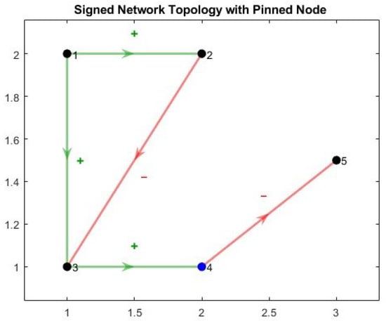
Figure 1. Signed network topology showing positive and negative edges, with the pinned node highlighted (blue).

• $a_{ij}>0$ for intra-group edges ($i,k\in {\mathcal{U}}_1$ or $i,k\in {\mathcal{U}}_2$),
• $a_{ij}<0$ for inter-group edges ($i\in {\mathcal{U}}_1$, $k\in {\mathcal{U}}_2$ or vice versa).

Node 4 belongs to ${\mathcal{U}}_2$ and is chosen as the pinned node in the leader–following case, which guarantees a directed spanning tree rooted at the leader (Assumption 3). Figure 1 shows the signed network topology of the 5-node graph: green arrows marked “+” denote cooperative (positive) links with $a_{ij}>0$, whereas red arrows marked “–” denote antagonistic (negative) links with $a_{ij}<0$. The pinned node (node 4) is highlighted in blue.

The mode-dependent system matrices are chosen as

$$\begin{array}{cccc}\hfill A_1& =\left(\begin{array}{ccc}0& -2& 0.8\\ 0.5& -1& 1\\ 0.1& -1& 0\end{array}\right),\hfill & \hfill A_2& =\left(\begin{array}{ccc}-0.3& -1.2& 0.5\\ 0.4& -0.9& 0.8\\ 0.2& -0.7& -0.1\end{array}\right),\hfill \\ \hfill B_1& =\left(\begin{array}{c}1\\ 0\\ 0\end{array}\right),\hfill & \hfill B_2& =\left(\begin{array}{c}1\\ 0.2\\ 0\end{array}\right),\hfill \\ \hfill D_1& =\left(100\right),\hfill & \hfill D_2& =\left(10.10\right).\hfill \end{array}$$

The scalar nonlinearity is

$$g\left(\nu \right)={\displaystyle \frac{1}{2}}\left(|\nu +1|-|\nu -1|\right),$$

(18)

and the feedback term entering the dynamics is $g\left(D_{\sigma \left(t\right)}{x}_i\left(t\right)\right)$. This nonlinearity is odd and sector-bounded, so Assumption 2 holds with a global sector bound $\eta =0.18$.

The semi-Markov process $\sigma \left(t\right)$ has two modes with transition probability matrix

$$\mathrm{\Pi }=\left(\begin{array}{cc}0.9& 0.1\\ 0.2& 0.8\end{array}\right),$$

and exponential sojourn-time distributions $F_i\left(\theta \right)=1-e^{-\theta /{\tau }_i}$ with means ${\tau }_1=2.5\mathrm{s}$ and ${\tau }_2=3\mathrm{s}$. The corresponding densities are $f_i\left(\theta \right)={\tau }_i^{-1}{e}^{-\theta /{\tau }_i}$, which are used in the stochastic LMI condition of Theorem 1.

5.2. Design of the Coupling Gain and LMI Verification

Following Remark 1, we choose the disagreement-space matrix $\Delta \in {\mathbb{R}}^{4\times 4}$ as

$$\Delta =\left(\begin{array}{cccc}0.2& 0& 0& 0\\ 0& 0.3& 0.21& 0\\ 0& 0.55& 0.24& 0.3\\ 0& 0.21& 0.35& 0.1\end{array}\right)>0,$$

and set $P_s=\Delta \otimes I_3$ and $T_s=I_1$ for both modes. For each $s\in \mathcal{S}$, we compute the bound matrix

$${\mathrm{\Lambda }}_s=\Delta \otimes (A_s+A_s^T)+{\displaystyle \frac{1}{2}}{\left(\Delta \otimes B_s+D_s\right)}^T\left(\Delta \otimes B_s+D_s\right),$$

and define $\mathrm{\Lambda }:={max}_{s\in \mathcal{S}}{\mathrm{\Lambda }}_s$. Numerically, the largest eigenvalue is ${\lambda }_{max}\left(\mathrm{\Lambda }\right)=2.7651$. Hence Theorem 1 requires the coupling gain to satisfy

$$\rho >{\displaystyle \frac{{\lambda }_{max}\left(\mathrm{\Lambda }\right)}{\eta }}\approx {\displaystyle \frac{2.7651}{0.18}}\approx 15.3618.$$

We therefore select

$$\rho =16,$$

which is safely above the theoretical lower bound.

The static quantizer is implemented as

$$q\left(x\right)=(I+\Sigma )x,\Sigma =\sigma I_3,$$

with $\sigma =0.05$, so that the diagonal perturbation matrix satisfies $|{\sigma }_k|\le \sigma$ as required in the analysis.

The quantized signal is generated according to the uncertainty model (6). In the simulations, we set the relative-error bound to $\overline{\delta }=0.05$ and use a diagonal perturbation ${\Sigma }_q\left(t\right)=\mathrm{diag}({\delta }_1\left(t\right),{\delta }_2\left(t\right),{\delta }_3\left(t\right))$ satisfying $|{\delta }_{\ell }\left(t\right)|\le \overline{\delta }$ for all ℓ and all t.

For the leader–following case, the pinning matrix is chosen as

$$D=\mathrm{diag}(0,0,0,1,0),$$

so that only node 4 is directly connected to the leader. The resulting matrix $\mathrm{\Phi }=\mathcal{L}+D$ is numerically verified to be a nonsingular M-matrix: all eigenvalues have positive real parts and ${\mathrm{\Phi }}^{-1}\ge 0$ entrywise, which matches Lemma 4 and ensures the dissipativity of the pinned interconnection.

The LMIs in Theorems 1 and 2 are solved using MATLAB’s LMI Toolbox. For the chosen $\rho$ and $\sigma$, feasible solutions $P_s>0$, $Q_s>0$, and $T_s>0$ are obtained for both modes, confirming that the stochastic LMI (7) and the mode-dependent inequality $S_s\le 0$ are satisfied.

For transparency and reproducibility, the feasible matrices obtained from the LMI solver are reported explicitly. Table 1 lists the mode-dependent matrices used to verify Theorem 1 (condition (7)) and Theorem 2 (condition (12)) for the selected design parameters $\rho =16$ and $\overline{\delta }=0.05$. The Lyapunov matrices in Theorem 1 satisfy $P_s=\Delta \otimes I_3$, and the corresponding $T_s$ are diagonal and positive.

Table 1. Feasible matrices used in the numerical LMI verification ($\rho =16$, $\overline{\delta }=0.05$).

Mode s	${\mathit{P}}_{\mathit{s}}$ (Theorem 1)	${\mathit{T}}_{\mathit{s}}$ (Theorem 1)
1	$P_1=\Delta \otimes I_3$	$T_1=1$
2	$P_2=\Delta \otimes I_3$	$T_2=1$
Mode $\mathbf{s}$	${\mathit{Q}}_{\mathit{s}}$ (Theorem 2)	${\mathit{T}}_{\mathit{s}}$ (Theorem 2)
1	$Q_1=I_3$	$T_1=1$
2	$Q_2=I_3$	$T_2=1$

For completeness, the explicit block form of $P_1=P_2=\Delta \otimes I_3$ is

$$P_1=P_2=\left(\begin{array}{cccc}0.2I_3& 0& 0& 0\\ 0& 0.3I_3& 0.21I_3& 0\\ 0& 0.55I_3& 0.24I_3& 0.3I_3\\ 0& 0.21I_3& 0.35I_3& 0.1I_3\end{array}\right),T_1=T_2=1,$$

where $I_3$ denotes the $3\times 3$ identity matrix.

• Topology matrix used in simulation. The signed adjacency matrix $\mathcal{A}=\left[a_{ij}\right]$ associated with Figure 1 is selected as

$$\mathcal{A}=\left[\begin{array}{ccccc}0& 1& -1& 0& 0\\ 1& 0& -1& 0& 0\\ -1& -1& 0& 1& 1\\ 0& 0& 1& 0& 1\\ 0& 0& 1& 1& 0\end{array}\right].$$

(19)

Accordingly, the degree matrix is $C=\mathrm{diag}(2,2,4,2,2)$ and the Laplacian is $\mathcal{L}=C-\mathcal{A}$, i.e.,

$$\mathcal{L}=\left[\begin{array}{ccccc}2& -1& 1& 0& 0\\ -1& 2& 1& 0& 0\\ 1& 1& 4& -1& -1\\ 0& 0& -1& 2& -1\\ 0& 0& -1& -1& 2\end{array}\right].$$

(20)

For the leader–following case, the pinning matrix is $D=\mathrm{diag}(0,0,0,1,0)$ and $\mathrm{\Phi }=\mathcal{L}+D$.

5.3. Simulation Setup

The closed-loop dynamics are simulated over the horizon $[0,20]$ with a fixed integration step of $\Delta t={10}^{-3}$ s. Initial conditions for the agents are drawn uniformly from the cube ${[-1,1]}^3$:

$$x_i\left(0\right)\sim \mathcal{U}\left({[-1,1]}^3\right),i=1,\dots ,5.$$

The bipartition is encoded by the diagonal matrix $\mathrm{\Gamma }=\mathrm{diag}(1,1,-1,-1,-1)$, and the transformed states ${\overline{x}}_i\left(t\right)={\gamma }_i{x}_i\left(t\right)$ are used to visualize bipartite synchronization. A single sample path of the semi-Markov process is generated from the kernel $(\mathrm{\Pi },\left\{F_i\right\})$ and used for both the leaderless and leader–following experiments. To avoid an uninformative realization with very few jumps, the semi-Markov sample path is regenerated until it contains multiple switching instants within $[0,T]$ (or, equivalently, the mean sojourn parameters are selected so that several mode transitions occur over the simulation horizon). The mode trajectory $\sigma \left(t\right)$ is plotted to make the switching behavior explicit.

For later analysis, we also track the semi-Markov mode profile $\sigma \left(t\right)$ along the trajectory. Figure 2 shows a typical realization of the switching pattern over $[0,20]$ s.

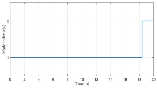
Figure 2. Sample path of the semi-Markov switching signal $\sigma \left(t\right)$ over the simulation horizon.

5.4. Leaderless Bipartite Synchronization

The distributed controller from Section III-A is implemented as

$$u_i\left(t\right)=-\rho \sum _{j=1}^N\left|a_{ij}\right|\left(q\left(x_i\left(t\right)\right)-sign\left(a_{ij}\right)q\left(x_j\left(t\right)\right)\right),$$

with $\rho =16$ and $q(·)$ defined above. Figure 3 shows the time evolution of the first component of the transformed states, ${\gamma }_i{x}_{i1}\left(t\right)$, for all five nodes.

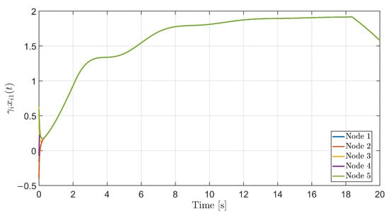
Figure 3. Trajectory convergence of the transformed states ${\gamma }_i{x}_{i1}\left(t\right)$, demonstrating bipartite leaderless synchronization under semi-Markov switching.

The trajectories of nodes 1 and 2 converge to a common profile, while nodes 3–5 converge to the same profile with opposite sign. The pattern remains stable in the presence of multiple mode transitions, which is in line with the conditions of Theorem 1.

5.5. Leader–Following Bipartite Synchronization

In the leader–following case, the leader evolves according to

$$\dot{y}\left(t\right)=A_{\sigma \left(t\right)}y\left(t\right)+B_{\sigma \left(t\right)}g\left(D_{\sigma \left(t\right)}y\left(t\right)\right),$$

with a randomly chosen initial condition $y\left(0\right)\in {[-1,1]}^3$. The mode-dependent leader–following controller from Section III-B is implemented as

$$\begin{array}{cc}\hfill u_i\left(t\right)=& -\rho \sum _{j=1}^N\left|a_{ij}\right|\left(q\left(x_i\left(t\right)\right)-sign\left(a_{ij}\right)q\left(x_j\left(t\right)\right)\right)\hfill \\ & -\sigma d_i\left(q\left(x_i\left(t\right)\right)-{\gamma }_{i}q\left(y\left(t\right)\right)\right),\hfill \end{array}$$

with the same $\rho =16$ and $\sigma =0.05$. Figure 4 displays the evolution of the bipartite leader–following errors $e_{i1}\left(t\right)={\gamma }_i{x}_{i1}\left(t\right)-y_1\left(t\right)$ for all nodes.

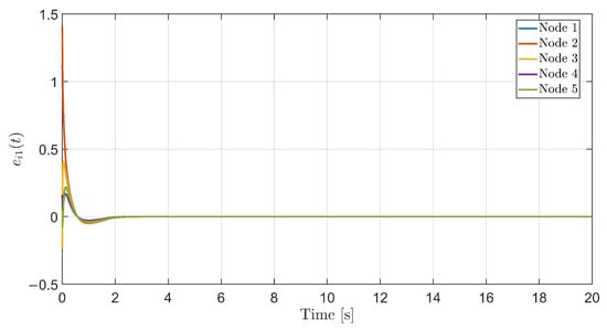
Figure 4. Leader–following bipartite synchronization under quantized pinning control: evolution of the first-component errors $e_{i1}\left(t\right)={\gamma }_i{x}_{i1}\left(t\right)-y_1\left(t\right)$.

The pinned node 4 converges most quickly to the leader, followed by the remaining nodes, which reach the same bipartite pattern through the signed network interactions. The error trajectories remain small after a short transient, in agreement with Theorem 2 and the M-matrix condition on $\mathrm{\Phi }=\mathcal{L}+D$.

5.6. Error Norms and Numerical Performance

To quantify the influence of the semi-Markov switching and the quantized feedback, we compute the Euclidean norms of the stacked errors in both cases. Let $E_L\left(t\right)$ denote the norm of the leaderless bipartite disagreement vector $\overline{e}\left(t\right)$, and let $E_F\left(t\right)$ denote the norm of the stacked leader–following errors. Figure 5 plots $E_L\left(t\right)$ and $E_F\left(t\right)$ for the same sample path of $\sigma \left(t\right)$.

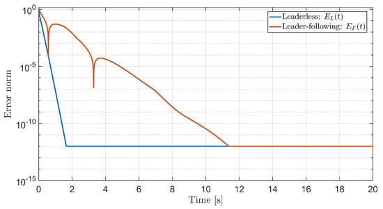
Figure 5. Error norms for leaderless and leader–following cases under semi-Markov switching: $E_L\left(t\right)$ (bipartite disagreement) and $E_F\left(t\right)$ (leader–following errors).

Both error norms decay rapidly. For the chosen parameters, a typical simulation run yields the performance values summarized in Table 2. The settling time $T_{\mathrm{settle}}$ is measured as the first time instant at which the corresponding error norm remains below ${10}^{-3}$ until the end of the simulation. The RMS errors are computed over the last 5 s of the horizon.

Table 2. Convergence performance under semi-Markov switching for $\rho =16$ (theoretical lower bound from Theorem 1).

Scenario	$\mathit{\rho }$	${\mathit{T}}_{\mathbf{settle}}$ [s]	RMS Error on $[15,20]$
Leaderless bipartite	16	$0.418$	0
Leader–following bipartite	16	$0.574$	0

The numerical values confirm that the coupling gain chosen from the analytical lower bound is sufficient to enforce fast bipartite synchronization in both the leaderless and leader–following settings, even in the presence of semi-Markov switching and quantization.

5.7. Comparative Study with Baseline Designs

To make the numerical study more informative, we also compare the proposed semi-Markov quantized design with three baseline settings that are often used in practice:

• Baseline 1 (ideal communication): the same distributed protocol but without quantization, i.e., $q\left(x\right)=x$ (equivalently ${\Sigma }_q\left(t\right)\equiv 0$). This isolates the effect of finite-precision communication.
• Baseline 2 (no pinning in leader–following): the leader–following protocol with $D=0$ (all $d_i=0$). This checks the role of pinning and the nonsingular M-matrix requirement on $\mathrm{\Phi }=\mathcal{L}+D$ in Lemma 4.
• Baseline 3 (Markov special case): exponential sojourn times (memoryless switching), which recovers the usual Markov jump setting as a special case of the semi-Markov framework.

All methods use the same signed topology, the same initial conditions, and the same coupling gain $\rho =16$ (unless stated otherwise). Performance is summarized using: (i) settling time $T_{\mathrm{set}}$ defined as the first time when the chosen error norm stays below ${10}^{-3}$, (ii) RMS error over the last 5 s, and (iii) the control-energy proxy ${\int }_0^T{\sum }_{i=1}^N{\parallel u_i\left(t\right)\parallel }^{2}dt$ (reported for the leader–following case). Comparative analysis are summarized in the Table 3.

Table 3. Comparison with baseline approaches (computed under identical initial conditions; Baseline 3 uses exponential sojourn times).

Method	Quantizer	Switching	Pinning	${\mathit{T}}_{\mathbf{set}}^{\mathbf{L}}$	${\mathit{T}}_{\mathbf{set}}^{\mathbf{F}}$	Energy
Proposed	yes	semi-Markov	yes	0.3770	2.8040	$5.3726\times {10}^1$
Baseline 1	no	semi-Markov	yes	0.3910	2.7990	$5.2540\times {10}^1$
Baseline 2	yes	semi-Markov	no	0.3770	N/C	$4.2187\times {10}^1$
Baseline 3	yes	Markov (exp.)	yes	0.3770	2.4980	$5.3726\times {10}^1$

In Baseline 2, the leader–following error does not converge (marked as N/C), which matches the reachability intuition behind Assumption 3 and the M-matrix role of $\mathrm{\Phi }=\mathcal{L}+D$. Figure 6 overlays the error norms for a direct visual comparison of the convergence rates.

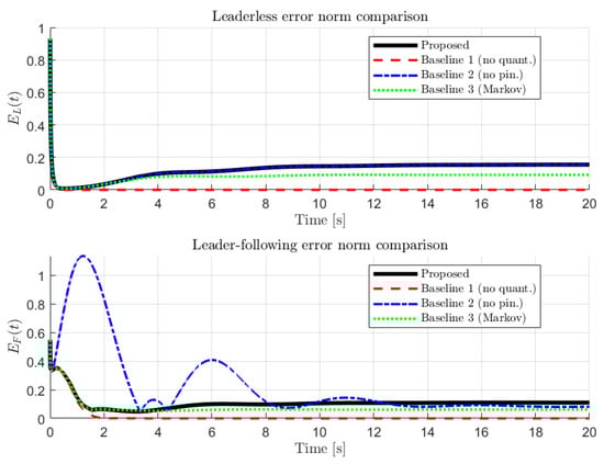
Figure 6. Error-norm comparison between the proposed method and the baseline approaches under the same initial conditions.

5.8. Computational Aspects

The feasibility conditions are verified by solving the semi-Markov LMI (7) (with ${\mathrm{\Omega }}_j$ given in (8)) and the mode-dependent LMI (13) for all $s\in \mathcal{S}$. The decision variables are $P_s\succ 0$ and diagonal $T_s\succ 0$ in Theorem 1, and $Q_s\succ 0$ and diagonal $T_s\succ 0$ in Theorem 2. Each inequality is a $2\times 2$ block LMI of order $n+r$, and the number of scalar unknowns per mode is $n(n+1)/2+r$ (and similarly for Theorem 2), hence the total scales linearly with $\left|\mathcal{S}\right|$. These LMIs are solved offline using a standard interior-point SDP solver (MATLAB LMI Toolbox in our case). Online implementation only requires local neighbor summations and matrix–vector multiplications.

6. Conclusions

This study proposed a bipartite synchronization framework for structurally balanced signed Lur’e networks governed by semi-Markovian jump switching. By integrating quantized feedback and selective pinning control, the approach effectively addresses communication constraints and stochastic mode-dependent dynamics. Sufficient conditions for achieving both leaderless and leader–following synchronization were derived in terms of linear matrix inequalities, enabling a computationally efficient controller design. Theoretical developments were validated through simulation results, which demonstrated robust convergence of synchronization trajectories across switching modes. The findings confirm the efficacy of the proposed control strategy in ensuring reliable bipartite coordination under realistic network uncertainties.

The present results employ a memoryless quantizer modeled by the uncertainty form in (6). A natural next step is to develop a dynamic zooming quantizer by introducing a scaling factor $\mu \left(t\right)$ and defining $q_{\mu }\left(x\right)=\mu \left(t\right)q(x/\mu \left(t\right))$, which preserves the same multiplicative uncertainty structure while allowing the effective quantization bound to vary with $\mu \left(t\right)$ and helping to avoid saturation.

Another direction is to combine quantization with event-triggered communication so that agents transmit only when a triggering rule is violated, reducing bandwidth while maintaining bipartite synchronization guarantees. It is also of interest to incorporate communication delays (constant or time-varying) in the signed coupling and pinning channels, and to derive delay-dependent semi-Markov LMI conditions. In addition, additive measurement/actuation noise and external disturbances can be included by augmenting the model with bounded-energy (or stochastic) noise terms and establishing mean-square or $H_{\infty }$-type performance bounds. Finally, extending the numerical study to larger networks and more general semi-Markov kernels (e.g., Weibull-type sojourn times) will help assess scalability and sensitivity to switching statistics.

References

- Wang, J.; Xing, M.; Cao, J.; Park, J.H.; Shen, H. H∞ bipartite synchronization of double-layer Markov switched cooperation–competition neural networks: A distributed dynamic event-triggered mechanism. IEEE Trans. Neural Netw. Learn. Syst. 2021, 34, 278–289. [Google Scholar] [CrossRef]
- Li, N.; Zheng, W.X. Bipartite synchronization of multiple memristor-based neural networks with antagonistic interactions. IEEE Trans. Neural Netw. Learn. Syst. 2020, 32, 1642–1653. [Google Scholar] [CrossRef] [PubMed]
- Shen, H.; Wang, X.; Duan, P.; Cao, J.; Wang, J. H∞ bipartite synchronization control of Markov jump cooperation–competition networks with reaction–diffusions. IEEE Trans. Cybern. 2022, 53, 6626–6635. [Google Scholar] [CrossRef] [PubMed]
- He, Q.; Ma, Y. Quantized adaptive pinning control for fixed/preassigned-time cluster synchronization of multi-weighted complex networks with stochastic disturbances. Nonlinear Anal. Hybrid Syst. 2022, 44, 101157. [Google Scholar] [CrossRef]
- Wang, J.; Liu, X. Cluster synchronization for multi-weighted and directed complex networks via pinning control. IEEE Trans. Circuits Syst. II Express Briefs 2021, 69, 1347–1351. [Google Scholar] [CrossRef]
- Hou, M.; He, Q.; Ma, Y. Quantized adaptive practical fixed-time synchronization of stochastic complex networks with actuator faults. Chaos Solitons Fractals 2024, 181, 114641. [Google Scholar] [CrossRef]
- Sun, Y.; Hu, C.; Yu, J.; Li, H.; Wen, S. Bipartite complete synchronization of fractional heterogeneous networks via quantized control without gauge transformation. IEEE Trans. Syst. Man Cybern. Syst. 2025, in press. [Google Scholar] [CrossRef]
- Vong, S.; Shi, C.; Yao, Z. Exponential synchronization of coupled inertial neural networks with mixed delays via weighted integral inequalities. Int. J. Robust Nonlinear Control 2020, 30, 7341–7354. [Google Scholar] [CrossRef]
- Ai, X. Adaptive robust bipartite consensus of high-order uncertain multi-agent systems over cooperation–competition networks. J. Frankl. Inst. 2020, 357, 1813–1831. [Google Scholar] [CrossRef]
- Zhang, H.; Chen, J. Bipartite consensus of multi-agent systems over signed graphs: State feedback and output feedback control approaches. Int. J. Robust Nonlinear Control 2017, 27, 3–14. [Google Scholar] [CrossRef]
- Meng, Y.; Zhang, H.; Wu, A. Leaderless output sign consensus of heterogeneous multi-agent systems over switching signed graphs. Sci. China Inf. Sci. 2023, 66, 190208. [Google Scholar] [CrossRef]
- Meng, D.; Du, M.; Jia, Y. Interval bipartite consensus of networked agents associated with signed digraphs. IEEE Trans. Autom. Control 2016, 61, 3755–3770. [Google Scholar] [CrossRef]
- Zhao, G.; Cui, H.; Hua, C. Hybrid event-triggered bipartite consensus control of multiagent systems and application to satellite formation. IEEE Trans. Autom. Sci. Eng. 2022, 20, 1760–1771. [Google Scholar] [CrossRef]
- Shen, H.; Men, Y.; Wu, Z.; Cao, J.; Lu, G. Network-based quantized control for fuzzy singularly perturbed semi-Markov jump systems and its application. IEEE Trans. Circuits Syst. I Regul. Pap. 2018, 66, 1130–1140. [Google Scholar] [CrossRef]
- Deng, Y.; Che, W. Fault-Tolerant Fuzzy Formation Control for a Class of Nonlinear Multi-Agent Systems Under Directed and Switching Topology. IEEE Trans. Syst. Man Cybern. Syst. 2021, 51, 5456–5465. [Google Scholar] [CrossRef]
- Shen, M.; Ma, Y.; Park, J.H.; Wang, L. Fuzzy Tracking Control for Markov Jump Systems With Mismatched Faults by Iterative Proportional-Integral Observers. IEEE Trans. Fuzzy Syst. 2022, 30, 542–554. [Google Scholar] [CrossRef]
- Reinders, J.; Giaccagli, M.; Hunnekens, B.; Astolfi, D.; Oomen, T.; van de Wouw, N. Repetitive control for Luré-type systems: Application to mechanical ventilation. IEEE Trans. Control Syst. Technol. 2023, 31, 1819–1829. [Google Scholar] [CrossRef]
- Kim, J.; Kim, H. Synchronization of Luré-type nonlinear systems in linear dynamical networks having fast convergence rate and large DC gain. Syst. Control Lett. 2020, 138, 104641. [Google Scholar] [CrossRef]
- Liu, H.; Li, N.; Sun, J.; Du, C. Dynamic event-triggered consensus of nonlinear Luré networks with directed switching topologies. IEEE Trans. Circuits Syst. II Express Briefs 2023, 71, 261–265. [Google Scholar]
- Wang, Y.; Lu, J.; Liang, J.; Cao, J.; Perc, M. Pinning synchronization of nonlinear coupled Luré networks under hybrid impulses. IEEE Trans. Circuits Syst. II Express Briefs 2018, 66, 432–436. [Google Scholar]
- Yang, J.; Huang, J.; He, X.; Wen, S. Bipartite synchronization of signed Luré network via quantized control. IEEE Trans. Circuits Syst. II Express Briefs 2023, 70, 2475–2479. [Google Scholar]
- Sun, W.; Li, B.; Guo, W.; Wen, S.; Wu, X. Interval bipartite synchronization of multiple neural networks in signed graphs. IEEE Trans. Neural Netw. Learn. Syst. 2022, 34, 10970–10979. [Google Scholar] [CrossRef] [PubMed]
- Rasappan, S.; Kumaravel, S.K.; Murugesan, R. Switching fuzzy sliding mode control of bipartite synchronization in signed Luré networks under quantized and pinning control. TechRxiv 2025. [Google Scholar] [CrossRef]
- Rasappan, S.; Kumaravel, S.K.; Murugesan, R. Bipartite synchronization for signed Luré networks via semi-Markovian jump switching and quantized pinning control. TechRxiv 2025. [Google Scholar] [CrossRef]
- Boyd, S.; El Ghaoui, L.; Feron, E.; Balakrishnan, V. Linear Matrix Inequalities in System and Control Theory; SIAM: Philadelphia, PA, USA, 1994. [Google Scholar]
- Liu, F.; Song, Q.; Wen, G.; Lu, J.; Cao, J. Bipartite synchronization of Luré network under signed digraph. Int. J. Robust Nonlinear Control 2018, 28, 6087–6105. [Google Scholar] [CrossRef]
- Mu, G.; Li, L.; Li, X. Quasi-bipartite synchronization of signed delayed neural networks under impulsive effects. Neural Netw. 2020, 129, 31–42. [Google Scholar] [CrossRef]
- Ren, W.; Beard, R.W. Consensus seeking in multiagent systems under dynamically changing interaction topologies. IEEE Trans. Autom. Control 2005, 50, 655–661. [Google Scholar] [CrossRef]
- Berman, A.; Plemmons, R.J. Nonnegative Matrices in the Mathematical Sciences; SIAM: Philadelphia, PA, USA, 1994. [Google Scholar]
Disclaimer/Publisher’s Note: The statements, opinions and data contained in all publications are solely those of the individual author(s) and contributor(s) and not of MDPI and/or the editor(s). MDPI and/or the editor(s) disclaim responsibility for any injury to people or property resulting from any ideas, methods, instructions or products referred to in the content. |
© 2026 by the authors. Licensee MDPI, Basel, Switzerland. This article is an open access article distributed under the terms and conditions of the Creative Commons Attribution (CC BY) license.