
A Brief Perspective on Deep Learning Approaches for 2D Semantic Segmentation


Abstract
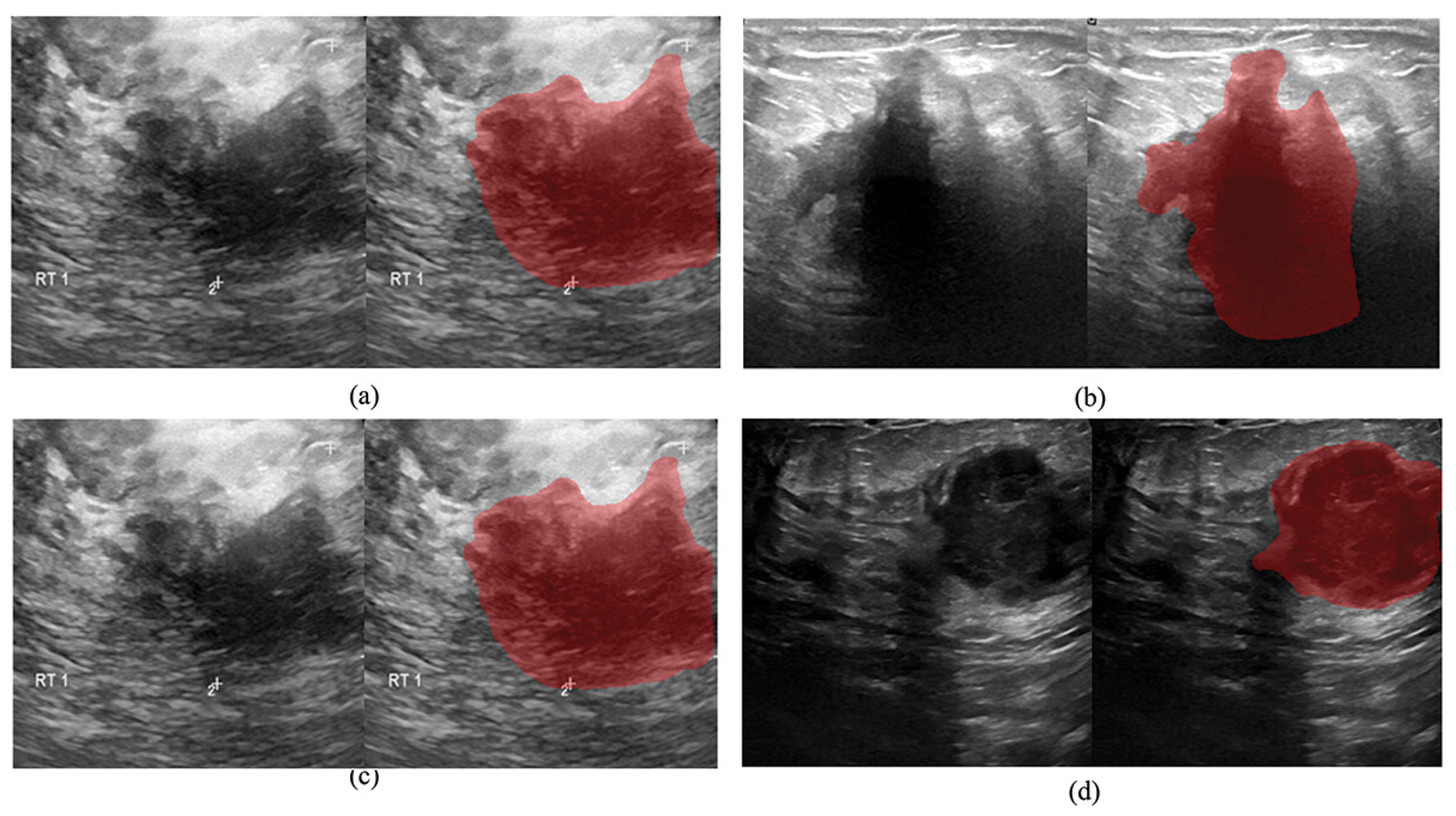
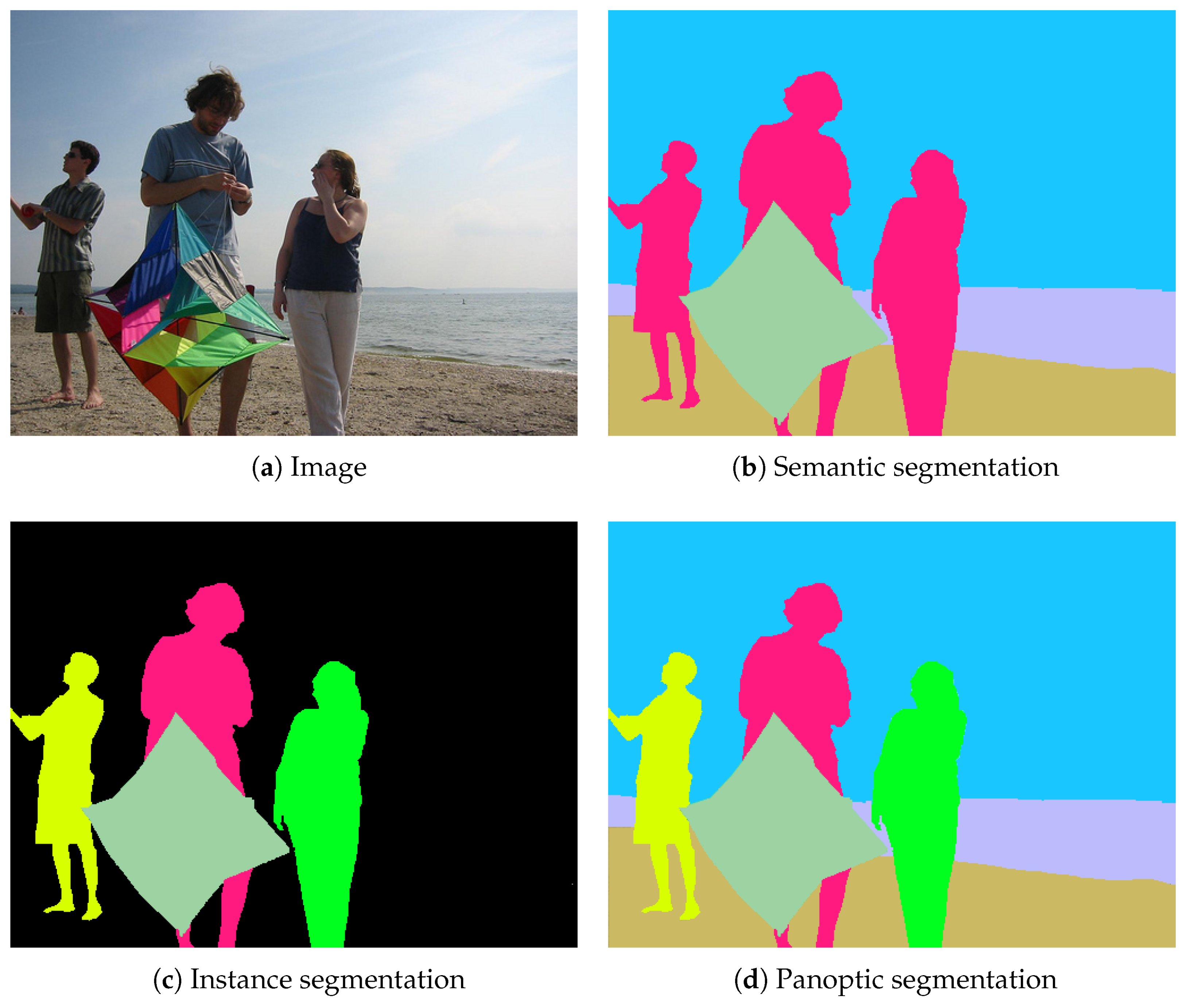
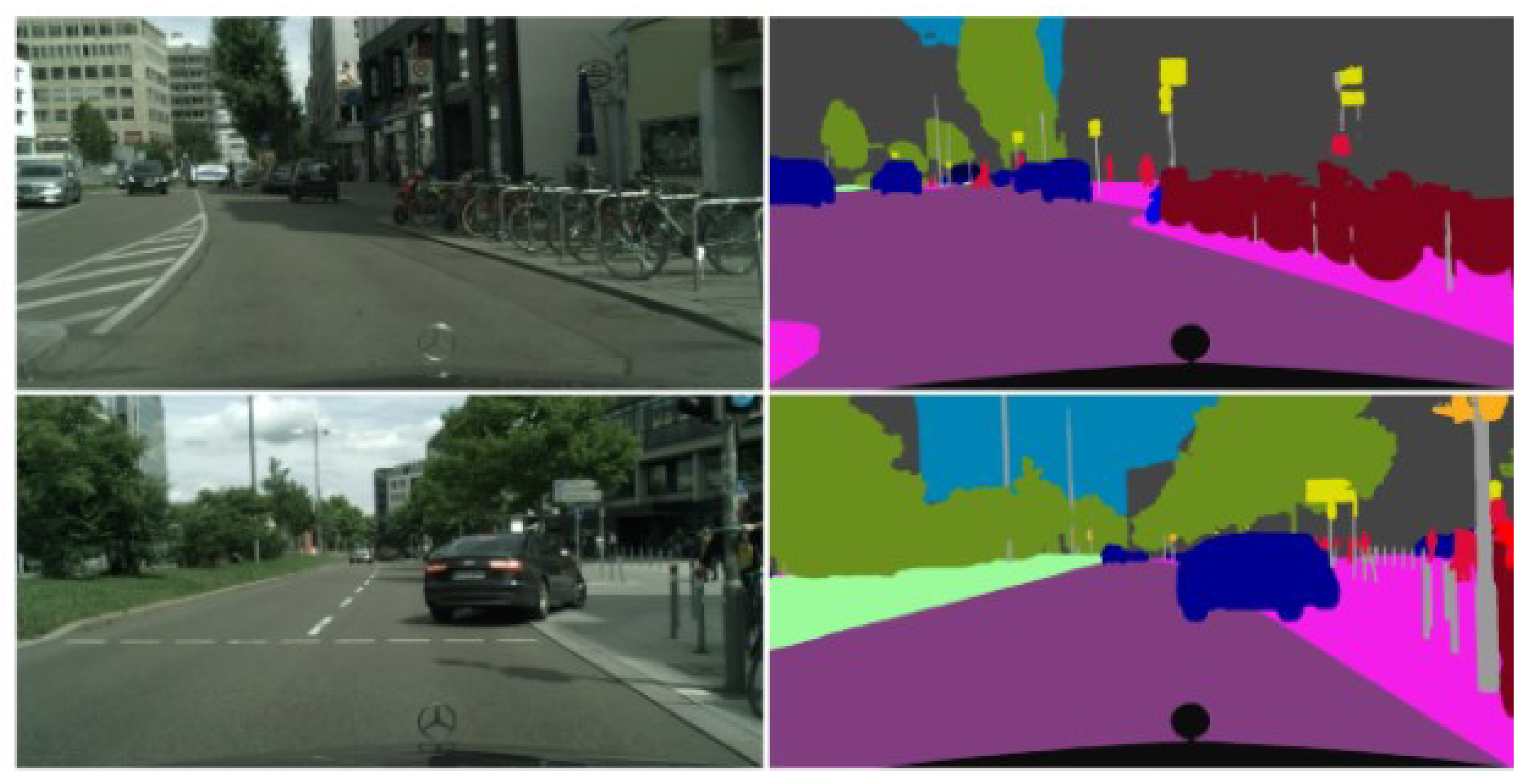
1. Introduction
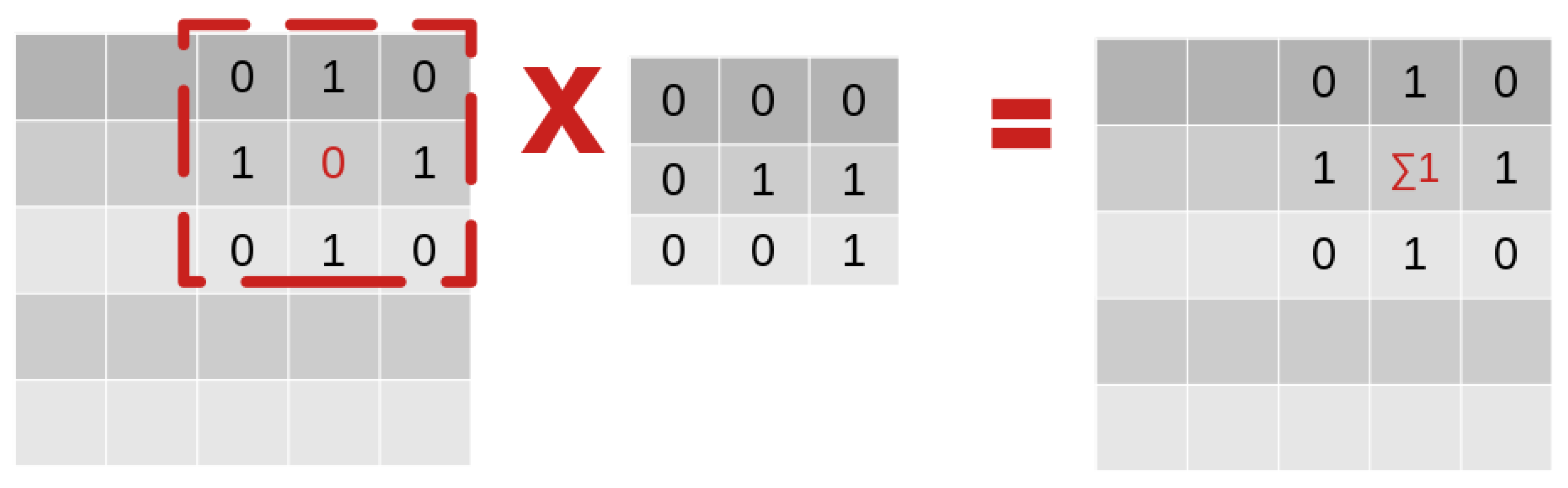
2. Fully Convolutional Neural Networks
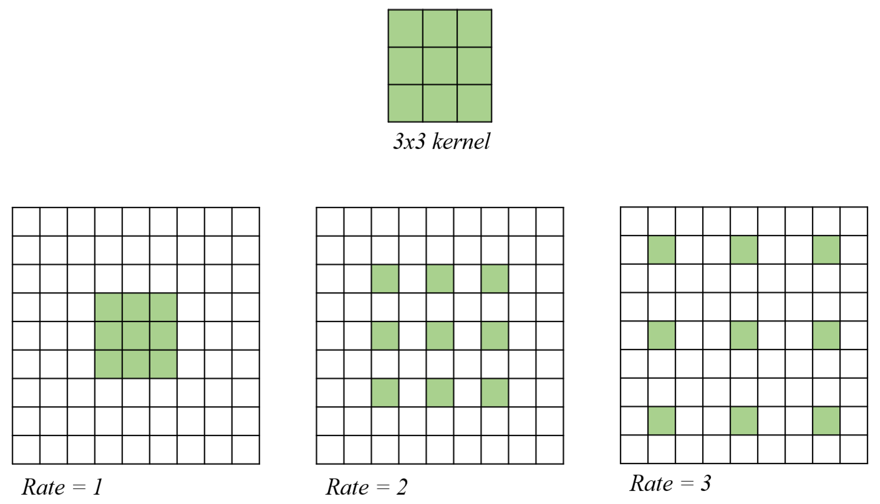
2.1. Atrous Convolution
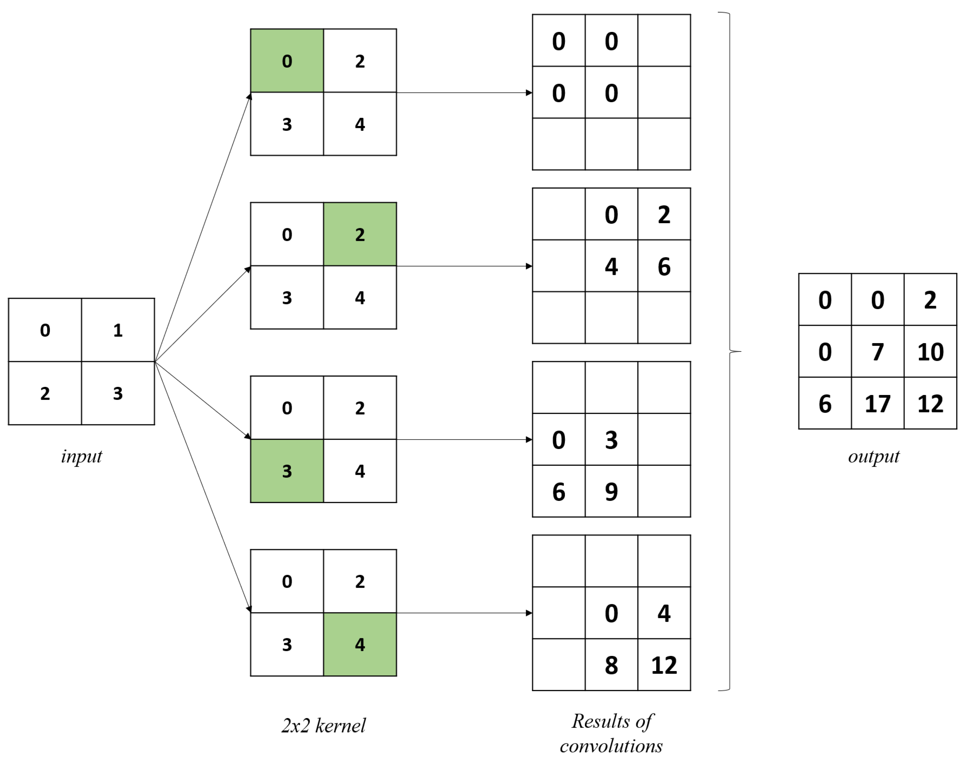
2.2. Transposed Convolution
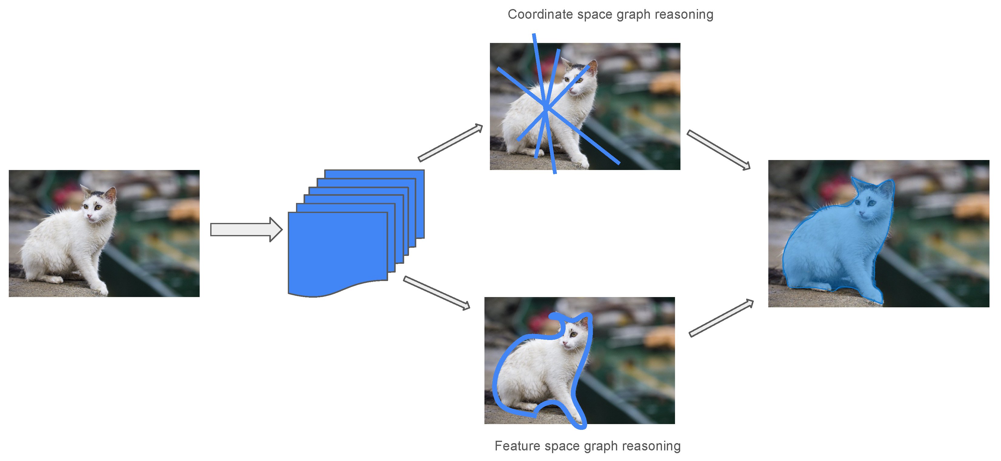
3. Graph Convolutional Networks
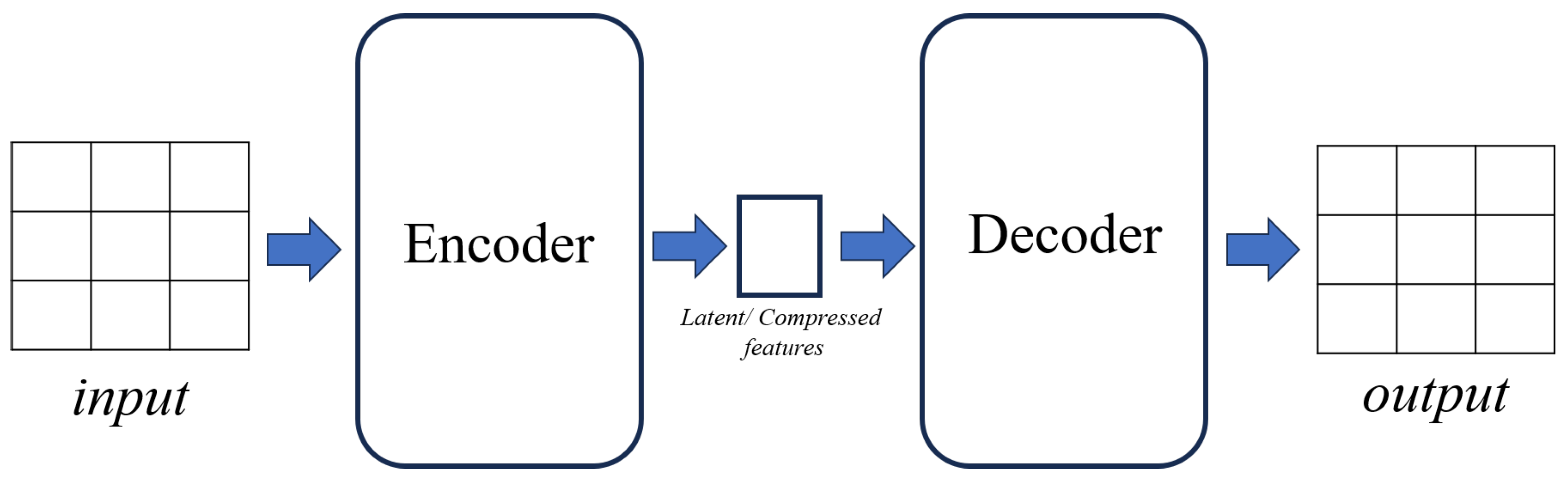
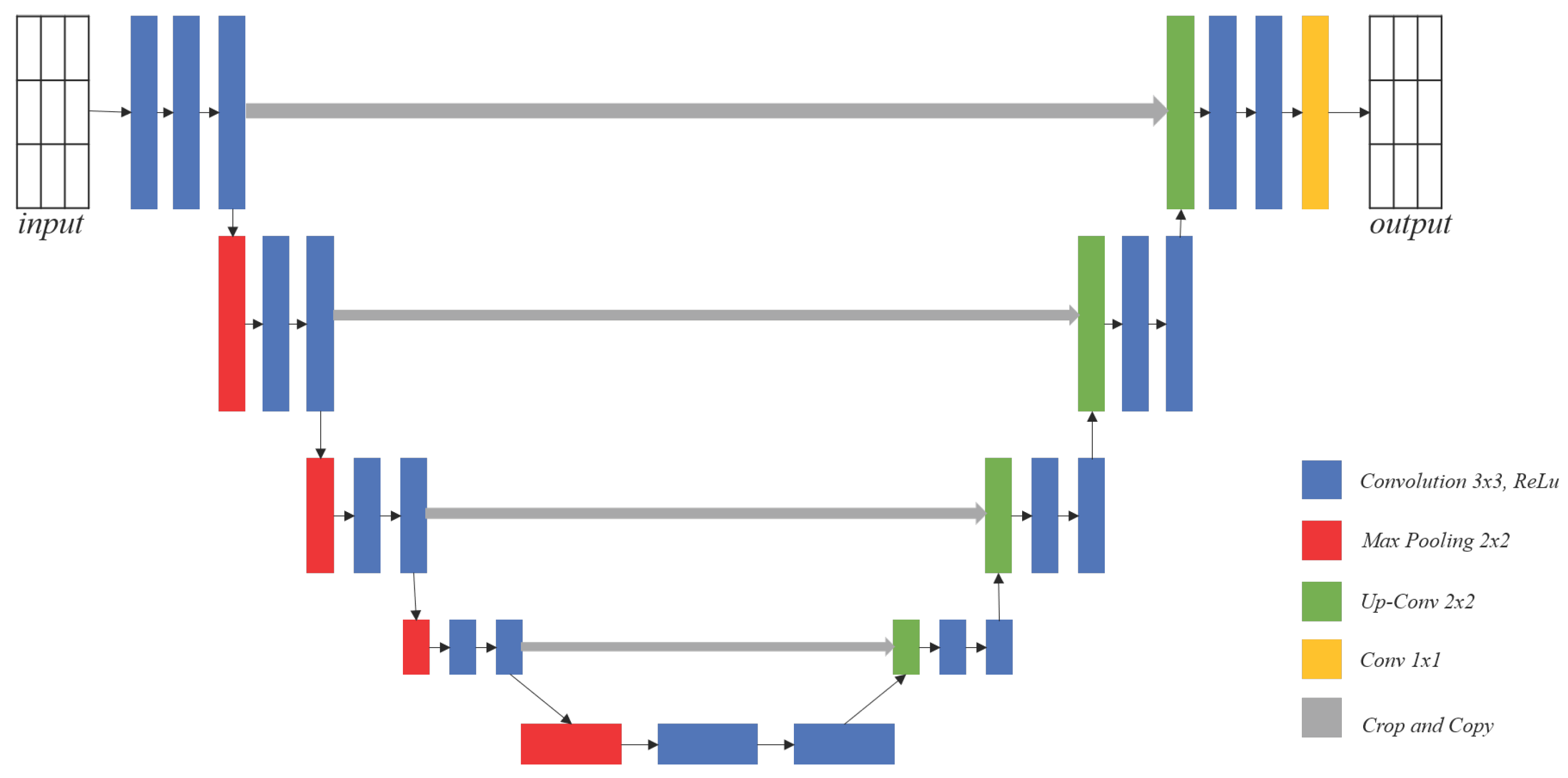
4. Encoder–Decoder Models and U-Nets
5. Feature Pyramid Networks
- The bottom-up pathway, responsible for the feed-forward computation of the convolutional network’s backbone. This pathway aggregates feature maps from multiple scales, scaling them by a factor of 2 to establish the feature hierarchy.
- Top-down pathways, which generate higher-resolution features by upsampling feature maps with lower spatial resolutions but richer semantic content from higher pyramid levels.
- Lateral connections, which merge maps from both the bottom-up and top-down pathways, ensuring that maps with matching spatial sizes are combined. The bottom-up pathway provides detailed information about lower-level semantics and precise object locations, while the top-down pathway contributes to higher-level semantic context. This merging process involves element-wise addition, followed by a convolution to reduce aliasing effects resulting from upsampling.
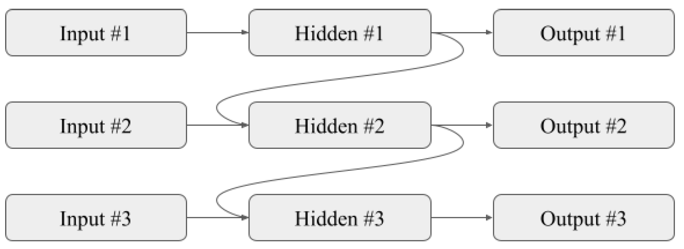
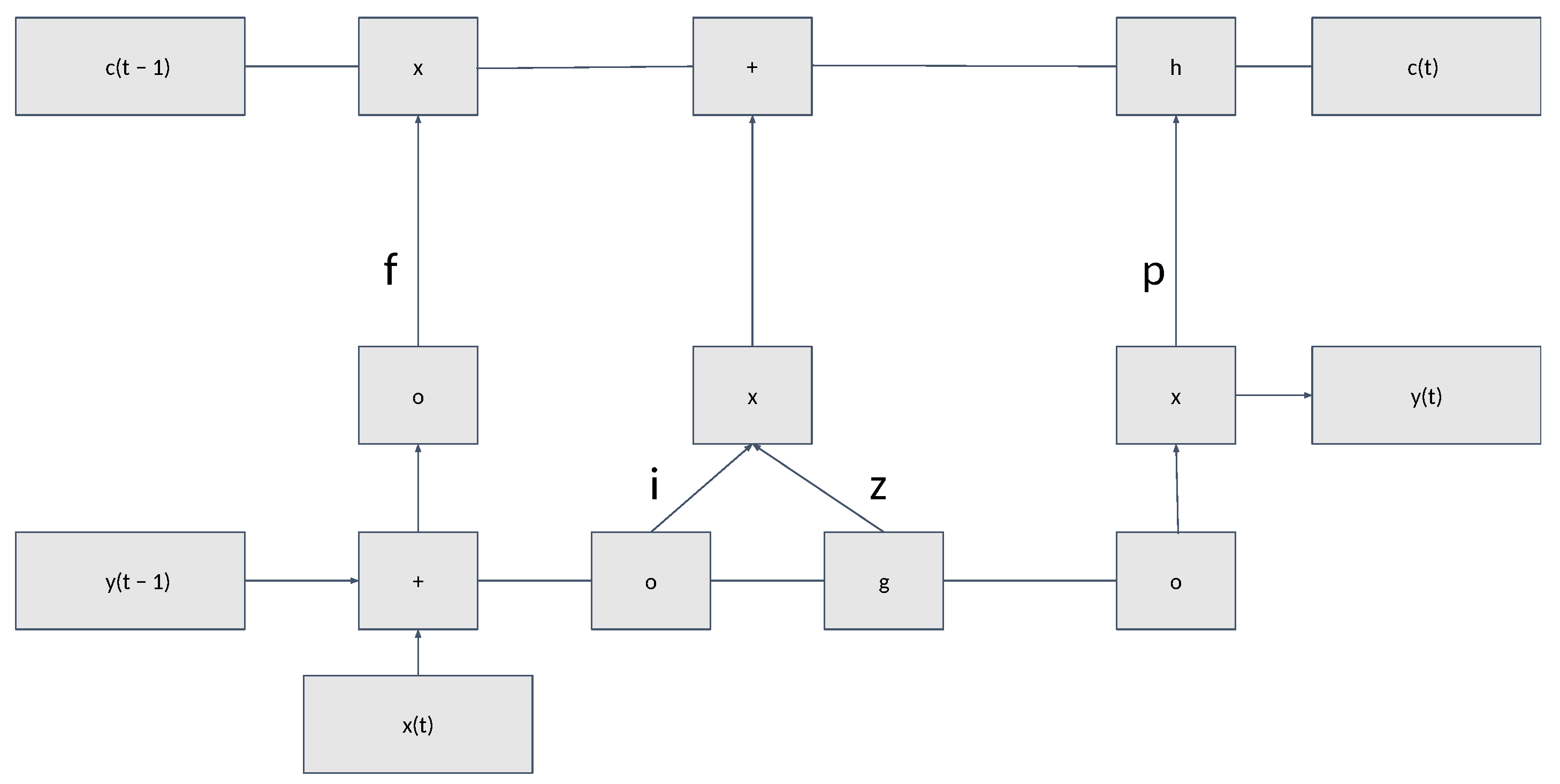
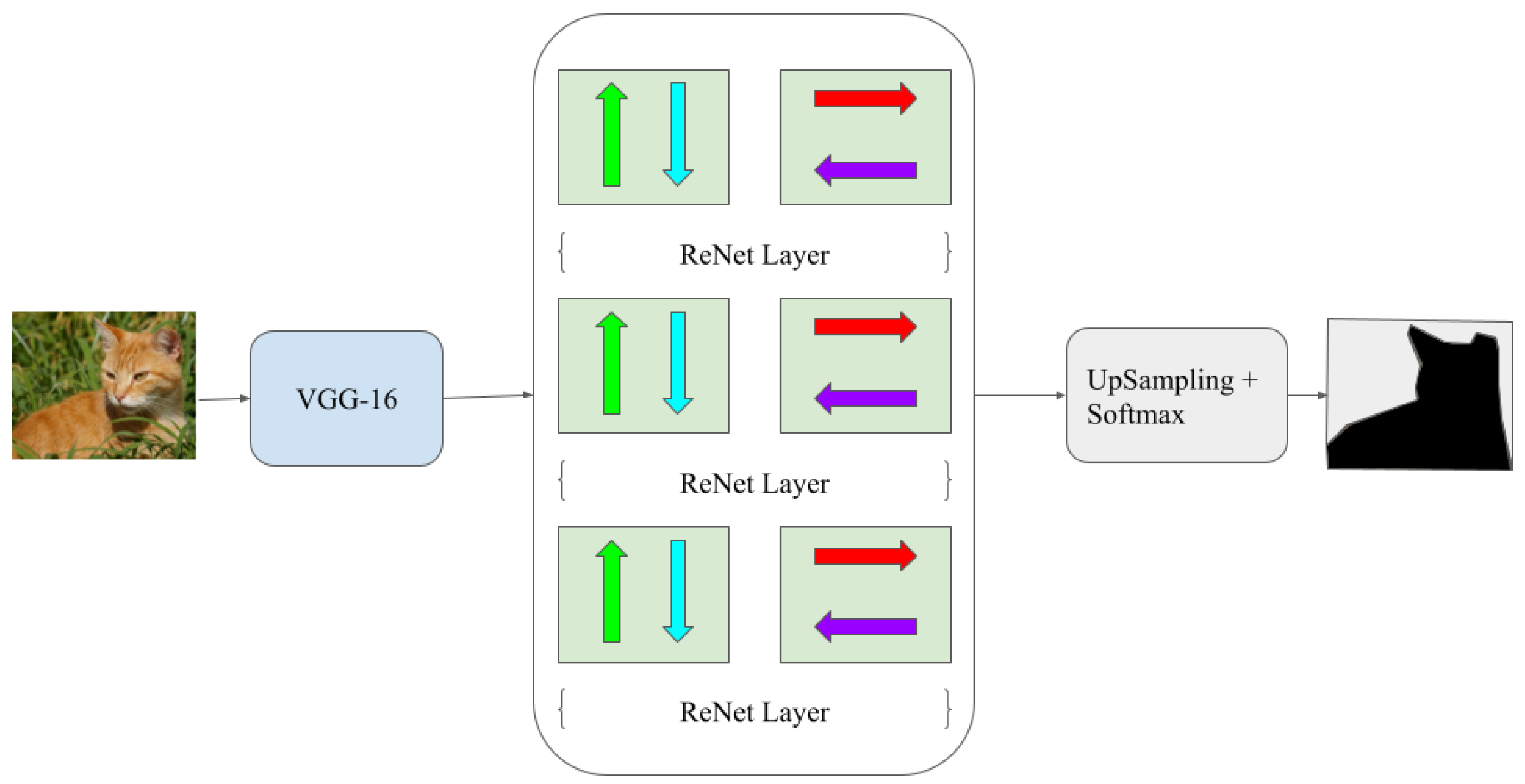
6. Recurrent Neural Networks
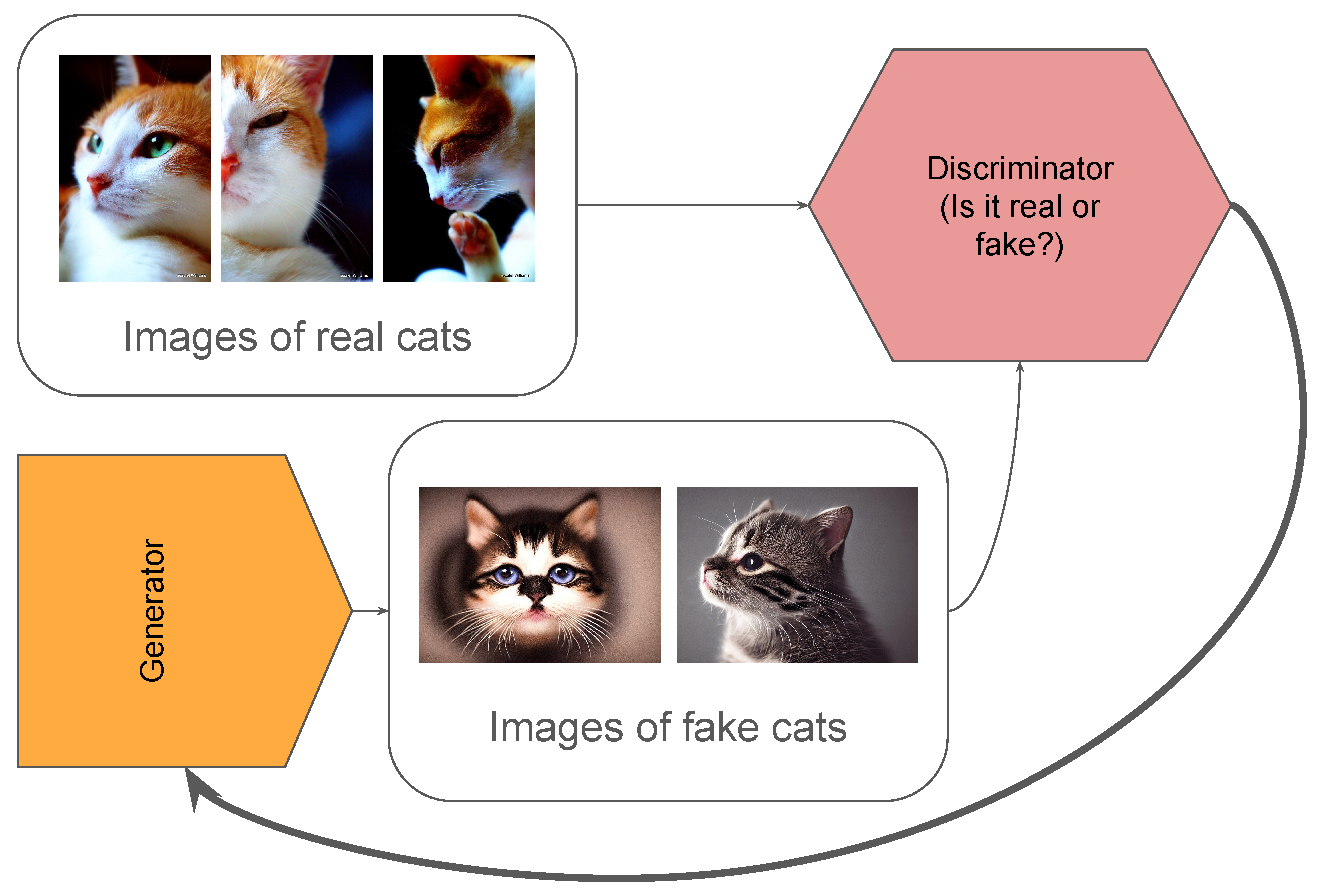
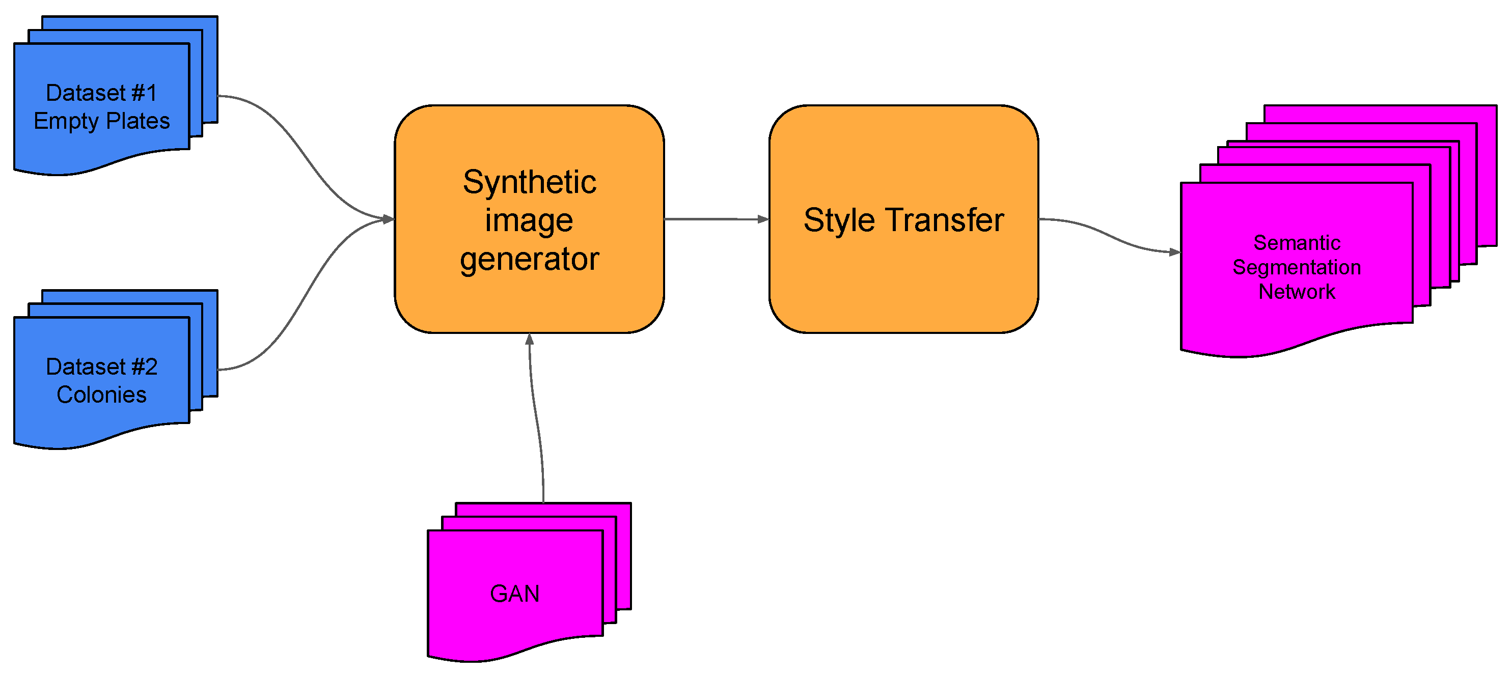
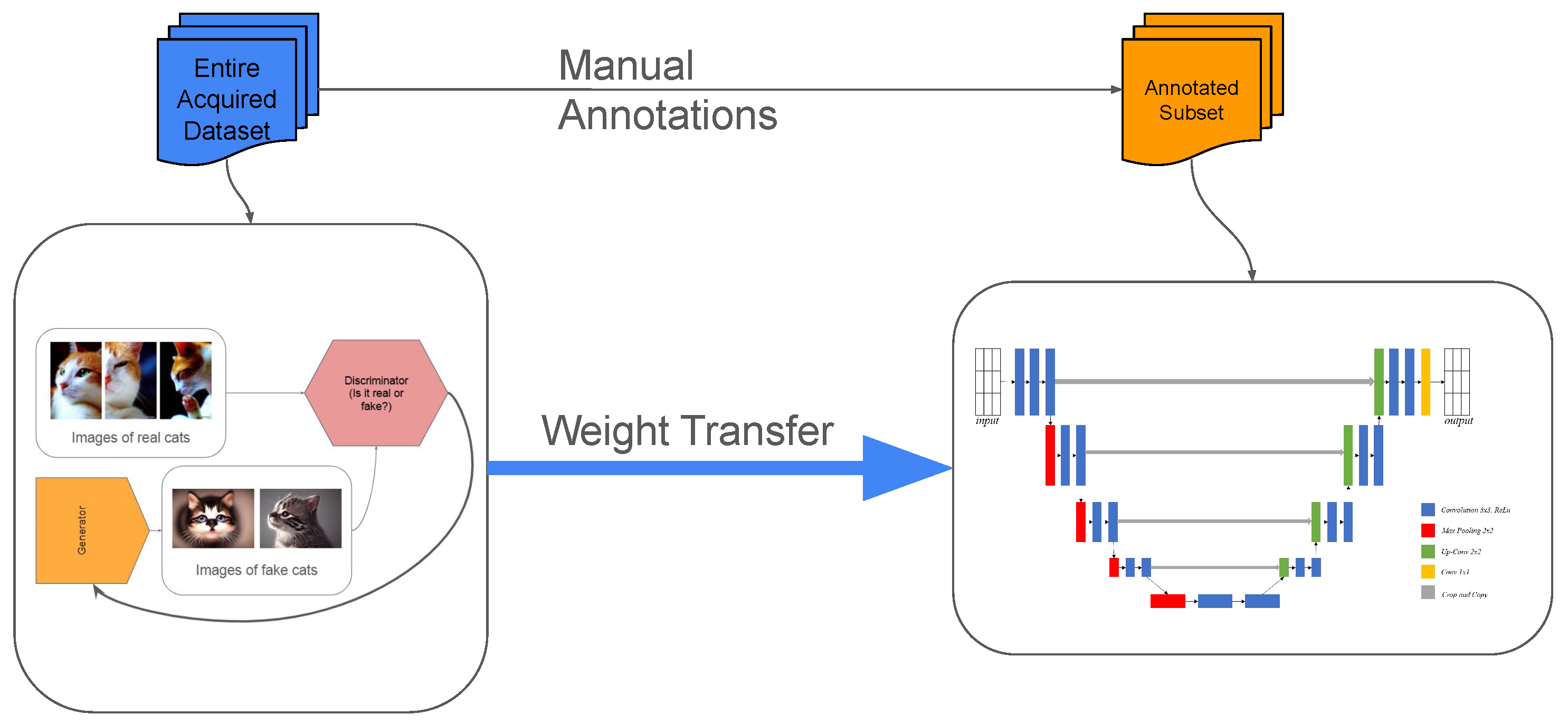
7. Generative Adversarial Networks
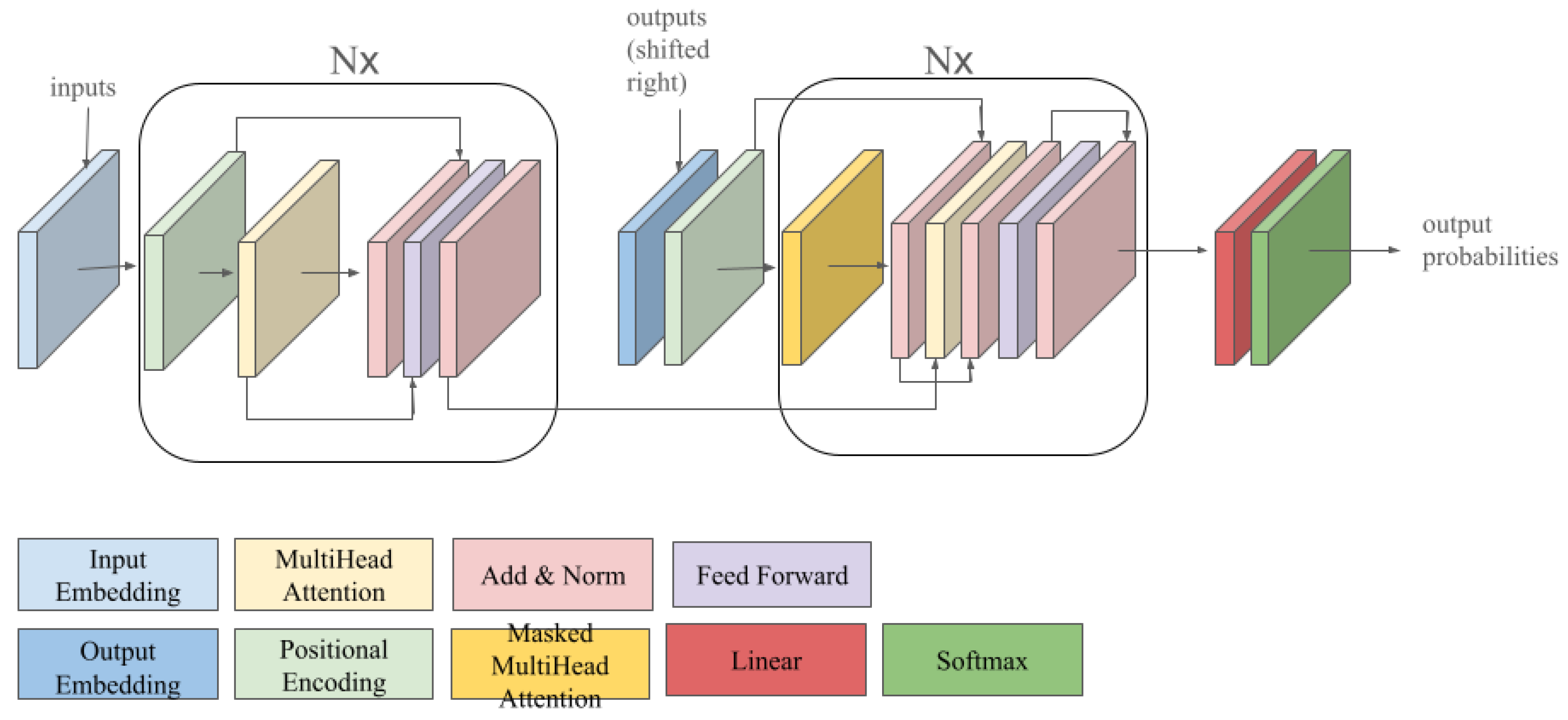
8. Attention-Based Networks
9. Spatial Transformer Networks
10. Neural Architecture Search
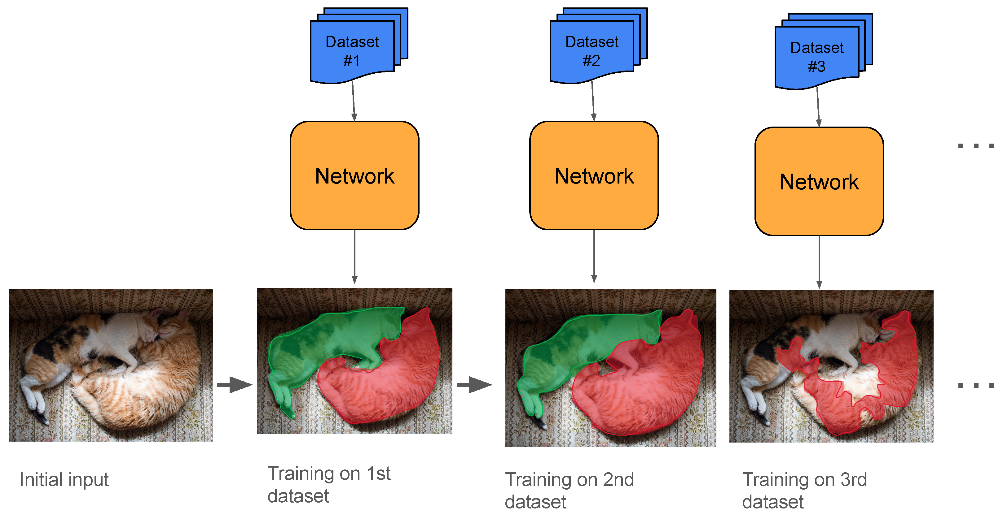
11. Continual Semantic Segmentation
12. Datasets

| Type | Dataset | Use Cases | Size | Classes | Notes |
|---|---|---|---|---|---|
| 2D | PASCAL VOC 2012 [119] | People, animals, vehicles, objects | 11,530 | 20 | 27,450 ROI and 6929 segmentations |
| PASCAL Context [120] | Objects, stuff, and hybrids | 10,103 | 400 | 9637 testing images | |
| MSCOCO [128] | Objects and stuff | 330K | 171 | 80 object classes and 91 stuff categories | |
| Cityscapes [17] | Street scenes and objects | 25K | 30 | 5K fine annotated and 20K coarsely annotated images | |
| ADE20K [129] | Scene images | 25,574 | 150 | Validation set of 2K images | |
| BSDS500 [130] | Contour and edge detection | 300 | Training set of 200 and test set of 100 images 12K hand labelled ROIs | ||
| YouTube-Objects [126] | YouTube videos | 10 | Each class has 9–24 videos of 3 s to 3 min length | ||
| CamVid [121] | Road driving scenes | 701 | 32 | Samples taken at 1 fps and 15 fps and manually annotated | |
| SBD [131] | Contour and edge detection | 11,355 | 20 | Images taken from PASCAL VOC 2011 | |
| PASCAL Part [127] | Body parts of each object | 10K+ | Testing set of 9637 images | ||
| OpenEarthMap [132] | Aereal images | 5000 | 8 | Over 64 regions, across 6 continents | |
| SIFTFlow [133] | Scene images | 33 | Two types of labelling: semantic and geometrical, has unannotated images | ||
| Stanford Background [134] | Scene images | 715 | 11 | 8 object classes and 3 geometric classes | |
| KITTI [122,123,124,125] | Road driving scenes | pixel-level and instance-level segmentation images and videos | |||
| BraTS [135] | Brain tumor segmentation | 775K+ | 4 | Multimodal MRI Dataset | |
| CHAOS [136] | Abdominal organ segmentation | 4.3K+ | 3 | CT and Multimodal MRI (T1-Dual, T2-SPIR) | |
| ISIC [137] | Skin lesion segmentation | 25K+ | 1 | Dermoscopic RGB Images | |
| DeepGlobe [138] | Satellite image segmentation | 24K+ | 7 | High-resolution Satellite RGB Imagery (0.5 m/pixel) | |
| SpaceNet [139] | Building footprint segmentation | 40K+ | 1 | Satellite RGB and Multispectral Imagery | |
| 2.5D | NYU-Depth V2 [140] | Indoor scenes | Video sequences of indoor scenes | ||
| SUN RGB-D [141] | RGB-D indoor scenes | 10,335 | Includes depth and segmentation masks | ||
| ScanNet [142] | Indoor scenes | 1513 | Instance level with 2D and 3D data | ||
| Stanford 2D-3D [143] | Indoor scenes | 70K+ | Includes raw sensor data, depth, surface normals, and semantic annotations |
13. Implementation Considerations
14. Metrics
14.1. Pixel Accuracy
14.2. Mean Pixel Accuracy
14.3. Intersection over Union
14.4. Mean IoU
14.5. Dice Coefficient
15. Discussion
16. Current and Future Directions in Semantic Segmentation
17. Conclusions
Author Contributions
Funding
Institutional Review Board Statement
Informed Consent Statement
Data Availability Statement
Conflicts of Interest
Abbreviations
| CNN | Convolutional Neural Network |
| CCTV | Closed Circuit Television |
| CRF | Conditional Random Fields |
| VSS | Video Semantic Segmentation |
| VPS | Video Panoptic Segmentation |
| FCN | Fully Convolutional Network |
| FPN | Feature Pyramid Network |
| NAS | Neural Architecture Search |
| GCN | Graph Convolutional Networks |
| CT | Computed Tomography |
| MRI | Magnetic Resonance Imaging |
| RNN | Recurrent Neural Network |
| GAN | Generative Adversarial Network |
| NLP | Natural Language Processing |
| STN | Spatial Transformer Network |
| RL | Reinforcement Learning |
| GPT | Generative Pre-training Transformer |
| PA | Pixel Accuracy |
| mPA | Mean Pixel Accuracy |
| IoU | Intersection Over Union |
| mIoU | Mean Intersection Over Union |
References
- Long, J.; Shelhamer, E.; Darrell, T. Fully convolutional networks for semantic segmentation. In Proceedings of the 2015 IEEE Conference on Computer Vision and Pattern Recognition (CVPR), Boston, MA, USA, 7–12 June 2015; pp. 3431–3440. [Google Scholar] [CrossRef]
- Xian, M.; Zhang, Y.; Cheng, H.; Xu, F.; Zhang, B.; Ding, J. Automatic Breast Ultrasound Image Segmentation: A Survey. arXiv 2017, arXiv:1704.01472. [Google Scholar] [CrossRef]
- Li, B.; Liu, S.; Xu, W.; Qiu, W. Real-time object detection and semantic segmentation for autonomous driving. In Proceedings of the MIPPR 2017: Automatic Target Recognition and Navigation, Xiangyang, China, 28–29 October 2017; Liu, J., Udupa, J.K., Hong, H., Eds.; International Society for Optics and Photonics, SPIE: California, CA, USA, 2018; Volume 10608, pp. 167–174. [Google Scholar] [CrossRef]
- Yasuno, M.; Yasuda, N.; Aoki, M. Pedestrian detection and tracking in far infrared images. In Proceedings of the 2004 Conference on Computer Vision and Pattern Recognition Workshop, Washington, DC, USA, 27 June–2 July 2004; p. 125. [Google Scholar] [CrossRef]
- Victoria Priscilla, C.; Agnes Sheila, S.P. Pedestrian Detection—A Survey. In Proceedings of the First International Conference on Innovative Computing and Cutting-Edge Technologies (ICICCT 2019), Istanbul, Turkey, 30–31 October 2019; Jain, L.C., Peng, S.L., Alhadidi, B., Pal, S., Eds.; Springer Nature: Cham, Switzerland, 2020; pp. 349–358. [Google Scholar] [CrossRef]
- Deepak, G.D.; Bhat, S.K. A comparative study of breast tumour detection using a semantic segmentation network coupled with different pretrained CNNs. Comput. Methods Biomech. Biomed. Eng. Imaging Vis. 2024, 12, 2373996. [Google Scholar] [CrossRef]
- Kohler, R. A segmentation system based on thresholding. Comput. Graph. Image Process. 1981, 15, 319–338. [Google Scholar] [CrossRef]
- Gómez, O.; González, J.A.; Morales, E.F. Image Segmentation Using Automatic Seeded Region Growing and Instance-Based Learning. In Progress in Pattern Recognition, Image Analysis and Applications; Rueda, L., Mery, D., Kittler, J., Eds.; Springer Nature: Berlin/Heidelberg, Germany, 2007; pp. 192–201. [Google Scholar]
- Roslin, A.; Marsh, M.; Provencher, B.; Mitchell, T.; Onederra, I.; Leonardi, C. Processing of micro-CT images of granodiorite rock samples using convolutional neural networks (CNN), Part II: Semantic segmentation using a 2.5D CNN. Miner. Eng. 2023, 195, 108027. [Google Scholar] [CrossRef]
- Lapa, P.A.F. Conditional Random Fields Improve the CNN-Based Prostate Cancer Classification Performance. Master’s Thesis, NOVA Information Management School, Lisbon, Portugal, 2019. [Google Scholar]
- Zhang, M.; Dong, B.; Li, Q. Deep active contour network for medical image segmentation. In Proceedings of the Medical Image Computing and Computer Assisted Intervention–MICCAI 2020: 23rd International Conference, Lima, Peru, 4–8 October 2020; Proceedings, Part IV 23. Springer: Berlin/Heidelberg, Germany, 2020; pp. 321–331. [Google Scholar]
- Li, P.; Xia, H.; Zhou, B.; Yan, F.; Guo, R. A Method to Improve the Accuracy of Pavement Crack Identification by Combining a Semantic Segmentation and Edge Detection Model. Appl. Sci. 2022, 12, 4714. [Google Scholar] [CrossRef]
- Yuheng, S.; Hao, Y. Image Segmentation Algorithms Overview. arXiv 2017, arXiv:1707.02051. [Google Scholar] [CrossRef]
- Tian, D.; Han, Y.; Wang, B.; Guan, T.; Gu, H.; Wei, W. Review of object instance segmentation based on deep learning. J. Electron. Imaging 2021, 31, 041205. [Google Scholar] [CrossRef]
- Kim, D.; Woo, S.; Lee, J.; Kweon, I.S. Video Panoptic Segmentation. arXiv 2020, arXiv:2006.11339. [Google Scholar] [CrossRef] [PubMed]
- Kirillov, A.; He, K.; Girshick, R.; Rother, C.; Dollar, P. Panoptic Segmentation. In Proceedings of the 2019 IEEE/CVF Conference on Computer Vision and Pattern Recognition (CVPR), Long Beach, CA, USA, 15–20 June 2019; pp. 9396–9405. [Google Scholar] [CrossRef]
- Cordts, M.; Omran, M.; Ramos, S.; Rehfeld, T.; Enzweiler, M.; Benenson, R.; Franke, U.; Roth, S.; Schiele, B. The Cityscapes Dataset for Semantic Urban Scene Understanding. In Proceedings of the 2016 IEEE Conference on Computer Vision and Pattern Recognition (CVPR), Las Vegas, NV, USA, 27–30 June 2016; pp. 3213–3223. [Google Scholar] [CrossRef]
- Prakash, V.J.; Nithya, L.M. A Survey on Semi-Supervised Learning Techniques. arXiv 2014, arXiv:1402.4645. [Google Scholar] [CrossRef]
- Chen, T.; Kornblith, S.; Swersky, K.; Norouzi, M.; Hinton, G.E. Big Self-Supervised Models are Strong Semi-Supervised Learners. In Advances in Neural Information Processing Systems; Larochelle, H., Ranzato, M., Hadsell, R., Balcan, M., Lin, H., Eds.; Curran Associates, Inc.: Red Hook, NY, USA, 2020; Volume 33, pp. 22243–22255. [Google Scholar]
- Ran, L.; Li, Y.; Liang, G.; Zhang, Y. Pseudo Labeling Methods for Semi-Supervised Semantic Segmentation: A Review and Future Perspectives. IEEE Trans. Circuits Syst. Video Technol. 2025, 35, 3054–3080. [Google Scholar] [CrossRef]
- Zhang, B.; Zhang, Y.; Li, Y.; Wan, Y.; Guo, H.; Zheng, Z.; Yang, K. Semi-supervised deep learning via transformation consistency regularization for remote sensing image semantic segmentation. IEEE J. Sel. Top. Appl. Earth Obs. Remote Sens. 2023, 16, 5782–5796. [Google Scholar] [CrossRef]
- Xie, J.; Shuai, B.; Hu, J.F.; Lin, J.; Zheng, W.S. Improving fast segmentation with teacher-student learning. arXiv 2018, arXiv:1810.08476. [Google Scholar] [CrossRef]
- Wang, W.; Zhou, T.; Porikli, F.; Crandall, D.J.; Gool, L.V. A Survey on Deep Learning Technique for Video Segmentation. arXiv 2021, arXiv:2107.01153. [Google Scholar] [CrossRef]
- Jung, S.; Heo, H.; Park, S.; Jung, S.U.; Lee, K. Benchmarking Deep Learning Models for Instance Segmentation. Appl. Sci. 2022, 12, 8856. [Google Scholar] [CrossRef]
- Portillo-Portillo, J.; Sanchez-Perez, G.; Toscano-Medina, L.K.; Hernandez-Suarez, A.; Olivares-Mercado, J.; Perez-Meana, H.; Velarde-Alvarado, P.; Orozco, A.L.S.; García Villalba, L.J. FASSVid: Fast and Accurate Semantic Segmentation for Video Sequences. Entropy 2022, 24, 942. [Google Scholar] [CrossRef] [PubMed]
- Chen, L.C.; Papandreou, G.; Schroff, F.; Adam, H. Rethinking Atrous Convolution for Semantic Image Segmentation. arXiv 2017, arXiv:1706.05587. [Google Scholar] [CrossRef]
- Chen, L.C.; Papandreou, G.; Kokkinos, I.; Murphy, K.; Yuille, A.L. Deeplab: Semantic image segmentation with deep convolutional nets, atrous convolution, and fully connected crfs. IEEE Trans. Pattern Anal. Mach. Intell. 2017, 40, 834–848. [Google Scholar] [CrossRef] [PubMed]
- Dumoulin, V.; Visin, F. A guide to convolution arithmetic for deep learning. arXiv 2018, arXiv:1603.07285. [Google Scholar] [CrossRef]
- Minaee, S.; Boykov, Y.; Porikli, F.; Plaza, A.; Kehtarnavaz, N.; Terzopoulos, D. Image Segmentation Using Deep Learning: A Survey. IEEE Trans. Pattern Anal. Mach. Intell. 2022, 44, 3523–3542. [Google Scholar] [CrossRef] [PubMed]
- Fukushima, K. Neocognitron: A self-organizing neural network model for a mechanism of pattern recognition unaffected by shift in position. Biol. Cybern. 2004, 36, 193–202. [Google Scholar] [CrossRef] [PubMed]
- Albawi, S.; Mohammed, T.A.; Al-Zawi, S. Understanding of a convolutional neural network. In Proceedings of the 2017 International Conference on Engineering and Technology (ICET), Antalya, Turkey, 21–23 August 2017; pp. 1–6. [Google Scholar] [CrossRef]
- Scherer, D.; Müller, A.; Behnke, S. Evaluation of Pooling Operations in Convolutional Architectures for Object Recognition. In Proceedings of the Artificial Neural Networks—ICANN 2010, Thessaloniki, Greece, 15–18 September 2010; Diamantaras, K., Duch, W., Iliadis, L.S., Eds.; Springer Nature: Cham, Switzerland, 2010; pp. 92–101. [Google Scholar] [CrossRef]
- O’Shea, K.; Nash, R. An Introduction to Convolutional Neural Networks. arXiv 2015, arXiv:1511.08458. [Google Scholar] [CrossRef]
- Estrach, J.B.; Szlam, A.; LeCun, Y. Signal recovery from Pooling Representations. In Proceedings of the 31st International Conference on Machine Learning, Bejing, China, 22–24 June 2014; Xing, E.P., Jebara, T., Eds.; Proceedings of Machine Learning Research. Volume 32, pp. 307–315. [Google Scholar]
- Wang, S.H.; Lv, Y.D.; Sui, Y.; Liu, S.; Wang, S.J.; Zhang, Y.D. Alcoholism detection by data augmentation and Convolutional Neural Network with stochastic pooling. J. Med. Syst. 2017, 42, 2. [Google Scholar] [CrossRef] [PubMed]
- Kassani, S.H.; Kassani, P.H.; Wesolowski, M.J.; Schneider, K.A.; Deters, R. Breast Cancer Diagnosis with Transfer Learning and Global Pooling. In Proceedings of the 2019 International Conference on Information and Communication Technology Convergence (ICTC), Jeju, Republic of Korea, 16–18 October 2019; pp. 519–524. [Google Scholar] [CrossRef]
- Lv, Y.; Ma, H.; Li, J.; Liu, S. Attention guided u-net with atrous convolution for accurate retinal vessels segmentation. IEEE Access 2020, 8, 32826–32839. [Google Scholar] [CrossRef]
- Qiao, S.; Chen, L.C.; Yuille, A. DetectoRS: Detecting objects with recursive feature pyramid and switchable atrous convolution. In Proceedings of the IEEE/CVF Conference on Computer Vision and Pattern Recognition, Nashville, TN, USA, 20–25 June 2021; pp. 10208–10219. [Google Scholar] [CrossRef]
- Kyrkou, C.; Theocharides, T. EmergencyNet: Efficient aerial image classification for drone-based emergency monitoring using atrous convolutional feature fusion. IEEE J. Sel. Top. Appl. Earth Obs. Remote Sens. 2020, 13, 1687–1699. [Google Scholar] [CrossRef]
- Zhou, Y.; Chang, H.; Lu, Y.; Lu, X. CDTNet: Improved image classification method using standard, Dilated and Transposed Convolutions. Appl. Sci. 2022, 12, 5984. [Google Scholar] [CrossRef]
- Odena, A.; Dumoulin, V.; Olah, C. Deconvolution and Checkerboard Artifacts. Distill 2016. [Google Scholar] [CrossRef]
- Gao, H.; Yuan, H.; Wang, Z.; Ji, S. Pixel transposed convolutional networks. IEEE Trans. Pattern Anal. Mach. Intell. 2019, 42, 1218–1227. [Google Scholar] [CrossRef] [PubMed]
- Zhang, S.; Tong, H.; Xu, J.; Maciejewski, R. Graph convolutional networks: A comprehensive review. Comput. Soc. Netw. 2019, 6, 11. [Google Scholar] [CrossRef] [PubMed]
- Tenenbaum, J.B.; de Silva, V.; Langford, J.C. A Global Geometric Framework for Nonlinear Dimensionality Reduction. Science 2000, 290, 2319–2323. [Google Scholar] [CrossRef] [PubMed]
- Roweis, S.T.; Saul, L.K. Nonlinear Dimensionality Reduction by Locally Linear Embedding. Science 2000, 290, 2323–2326. [Google Scholar] [CrossRef] [PubMed]
- Belkin, M.; Niyogi, P. Laplacian Eigenmaps and Spectral Techniques for Embedding and Clustering. In Advances in Neural Information Processing Systems; Dietterich, T., Becker, S., Ghahramani, Z., Eds.; MIT Press: Cambridge, MA, USA, 2001; Volume 14. [Google Scholar]
- Perozzi, B.; Al-Rfou, R.; Skiena, S. DeepWalk: Online Learning of Social Representations. arXiv 2014, arXiv:1403.6652. [Google Scholar] [CrossRef]
- Grover, A.; Leskovec, J. node2vec: Scalable Feature Learning for Networks. arXiv 2016, arXiv:1607.00653. [Google Scholar] [CrossRef]
- Wu, F.; Souza, A.; Zhang, T.; Fifty, C.; Yu, T.; Weinberger, K. Simplifying Graph Convolutional Networks. In Proceedings of the 36th International Conference on Machine Learning, PMLR, Long Beach, CA, USA, 9–15 June 2019; Chaudhuri, K., Salakhutdinov, R., Eds.; Proceedings of Machine Learning Research. Volume 97, pp. 6861–6871. [Google Scholar]
- Chen, M.; Wei, Z.; Huang, Z.; Ding, B.; Li, Y. Simple and Deep Graph Convolutional Networks. In Proceedings of the 37th International Conference on Machine Learning, PMLR, Online, 13–18 July 2020; Daumé, H., Singh, A., Eds.; Proceedings of Machine Learning Research. Volume 119, pp. 1725–1735. [Google Scholar]
- Zhang, L.; Li, X.; Arnab, A.; Yang, K.; Tong, Y.; Torr, P.H.S. Dual Graph Convolutional Network for Semantic Segmentation. arXiv 2019, arXiv:1909.06121. [Google Scholar] [CrossRef]
- Bian, T.; Xiao, X.; Xu, T.; Zhao, P.; Huang, W.; Rong, Y.; Huang, J. Rumor Detection on Social Media with Bi-Directional Graph Convolutional Networks. Proc. AAAI Conf. Artif. Intell. 2020, 34, 549–556. [Google Scholar] [CrossRef]
- Schulte-Sasse, R.; Budach, S.; Hnisz, D.; Marsico, A. Graph Convolutional Networks Improve the Prediction of Cancer Driver Genes. In Proceedings of the Artificial Neural Networks and Machine Learning—ICANN 2019: Workshop and Special Sessions, Munich, Germany, 17–19 September 2019; Tetko, I.V., Kůrková, V., Karpov, P., Theis, F., Eds.; Springer Nature: Cham, Switzerland, 2019; pp. 658–668. [Google Scholar] [CrossRef]
- Wang, H.; Zhao, M.; Xie, X.; Li, W.; Guo, M. Knowledge Graph Convolutional Networks for Recommender Systems. In Proceedings of the The World Wide Web Conference (WWW ’19), San Francisco, CA, USA, 13–17 May 2019; pp. 3307–3313. [Google Scholar] [CrossRef]
- Sun, M.; Zhao, S.; Gilvary, C.; Elemento, O.; Zhou, J.; Wang, F. Graph convolutional networks for computational drug development and discovery. Briefings Bioinform. 2019, 21, 919–935. [Google Scholar] [CrossRef] [PubMed]
- Yao, L.; Mao, C.; Luo, Y. Graph Convolutional Networks for Text Classification. Proc. AAAI Conf. Artif. Intell. 2019, 33, 7370–7377. [Google Scholar] [CrossRef]
- Ghosh, S.; Das, N.; Das, I.; Maulik, U. Understanding Deep Learning Techniques for Image Segmentation. arXiv 2019, arXiv:1907.06119. [Google Scholar] [CrossRef]
- Oktay, O.; Schlemper, J.; Folgoc, L.L.; Lee, M.C.H.; Heinrich, M.P.; Misawa, K.; Mori, K.; McDonagh, S.G.; Hammerla, N.Y.; Kainz, B.; et al. Attention U-Net: Learning Where to Look for the Pancreas. arXiv 2018, arXiv:1804.03999. [Google Scholar] [CrossRef]
- Alom, M.Z.; Yakopcic, C.; Hasan, M.; Taha, T.M.; Asari, V.K. Recurrent residual U-Net for medical image segmentation. J. Med. Imaging 2019, 6, 014006. [Google Scholar] [CrossRef] [PubMed]
- Chen, J.; Lu, Y.; Yu, Q.; Luo, X.; Adeli, E.; Wang, Y.; Lu, L.; Yuille, A.L.; Zhou, Y. TransUNet: Transformers Make Strong Encoders for Medical Image Segmentation. arXiv 2021, arXiv:2102.04306. [Google Scholar] [CrossRef]
- Alom, M.Z.; Hasan, M.; Yakopcic, C.; Taha, T.M.; Asari, V.K. Recurrent Residual Convolutional Neural Network based on U-Net (R2U-Net) for Medical Image Segmentation. arXiv 2018, arXiv:1802.06955. [Google Scholar] [CrossRef]
- Lin, T.Y.; Dollár, P.; Girshick, R.; He, K.; Hariharan, B.; Belongie, S. Feature Pyramid Networks for Object Detection. arXiv 2017, arXiv:1612.03144. [Google Scholar] [CrossRef]
- Hu, M.; Li, Y.; Fang, L.; Wang, S. A2-FPN: Attention Aggregation Based Feature Pyramid Network for Instance Segmentation. In Proceedings of the IEEE/CVF Conference on Computer Vision and Pattern Recognition (CVPR), Nashville, TN, USA, 20–25 June 2021; pp. 15338–15347. [Google Scholar] [CrossRef]
- Kirillov, A.; Girshick, R.; He, K.; Dollar, P. Panoptic Feature Pyramid Networks. In Proceedings of the IEEE/CVF Conference on Computer Vision and Pattern Recognition (CVPR), Long Beach, CA, USA, 15–20 June 2019; pp. 6392–6401. [Google Scholar] [CrossRef]
- Rumelhart, D.E.; Hinton, G.E.; Williams, R.J. Learning representations by back-propagating errors. Nature 1986, 323, 533–536. [Google Scholar] [CrossRef]
- Ribeiro, A.H.; Tiels, K.; Aguirre, L.A.; Schön, T. Beyond exploding and vanishing gradients: Analysing RNN training using attractors and smoothness. In Proceedings of the Twenty Third International Conference on Artificial Intelligence and Statistics, PMLR, Online, 26–28 August 2020; Chiappa, S., Calandra, R., Eds.; Proceedings of Machine Learning Research. Volume 108, pp. 2370–2380. [Google Scholar]
- Hochreiter, S.; Schmidhuber, J. Long Short-Term Memory. Neural Comput. 1997, 9, 1735–1780. [Google Scholar] [CrossRef] [PubMed]
- Cho, K.; van Merrienboer, B.; Gülçehre, Ç.; Bougares, F.; Schwenk, H.; Bengio, Y. Learning Phrase Representations using RNN Encoder-Decoder for Statistical Machine Translation. arXiv 2014, arXiv:1406.1078. [Google Scholar] [CrossRef]
- Miao, Y.; Gowayyed, M.; Metze, F. EESEN: End-to-end speech recognition using deep RNN models and WFST-based decoding. In Proceedings of the 2015 IEEE Workshop on Automatic Speech Recognition and Understanding (ASRU), Scottsdale, AZ, USA, 13–17 December 2015; pp. 167–174. [Google Scholar] [CrossRef]
- Mikolov, T.; Kombrink, S.; Burget, L.; Černocký, J.; Khudanpur, S. Extensions of recurrent neural network language model. In Proceedings of the 2011 IEEE International Conference on Acoustics, Speech and Signal Processing (ICASSP), Prague, Czech Republic, 22–27 May 2011; pp. 5528–5531. [Google Scholar] [CrossRef]
- Li, D.; Qian, J. Text sentiment analysis based on long short-term memory. In Proceedings of the 2016 First IEEE International Conference on Computer Communication and the Internet (ICCCI), Wuhan, China, 13–15 October 2016; pp. 471–475. [Google Scholar] [CrossRef]
- Visin, F.; Romero, A.; Cho, K.; Matteucci, M.; Ciccone, M.; Kastner, K.; Bengio, Y.; Courville, A. ReSeg: A Recurrent Neural Network-Based Model for Semantic Segmentation. In Proceedings of the 2016 IEEE Conference on Computer Vision and Pattern Recognition Workshops (CVPRW), Las Vegas, NV, USA, 26 June–1 July 2016; pp. 426–433. [Google Scholar] [CrossRef]
- Simonyan, K.; Zisserman, A. Very Deep Convolutional Networks for Large-Scale Image Recognition. In Proceedings of the 3rd International Conference on Learning Representations, ICLR 2015, San Diego, CA, USA, 7–9 May 2015; Bengio, Y., LeCun, Y., Eds.; ICLR: Appleton, WI, USA, 2015. [Google Scholar]
- Goodfellow, I.; Pouget-Abadie, J.; Mirza, M.; Xu, B.; Warde-Farley, D.; Ozair, S.; Courville, A.; Bengio, Y. Generative Adversarial Nets. In Advances in Neural Information Processing Systems; Ghahramani, Z., Welling, M., Cortes, C., Lawrence, N., Weinberger, K., Eds.; Curran Associates, Inc.: Red Hook, NY, USA, 2014; Volume 27. [Google Scholar]
- Zhang, X.; Jian, W.; Chen, Y.; Yang, S. Deform-GAN: An Unsupervised Learning Model for Deformable Registration. arXiv 2020, arXiv:2002.11430. [Google Scholar] [CrossRef]
- Dai, Z.; Yang, Z.; Yang, F.; Cohen, W.W.; Salakhutdinov, R.R. Good Semi-supervised Learning That Requires a Bad GAN. In Advances in Neural Information Processing Systems; Guyon, I., Luxburg, U.V., Bengio, S., Wallach, H., Fergus, R., Vishwanathan, S., Garnett, R., Eds.; Curran Associates, Inc.: Red Hook, NY, USA, 2017; Volume 30. [Google Scholar]
- Aggarwal, A.; Mittal, M.; Battineni, G. Generative adversarial network: An overview of theory and applications. Int. J. Inf. Manag. Data Insights 2021, 1, 100004. [Google Scholar] [CrossRef]
- Zhan, F.; Zhu, H.; Lu, S. Spatial Fusion GAN for Image Synthesis. In Proceedings of the IEEE/CVF Conference on Computer Vision and Pattern Recognition (CVPR), Long Beach, CA, USA, 15–20 June 2019. [Google Scholar] [CrossRef]
- Tran, N.T.; Tran, V.H.; Nguyen, N.B.; Nguyen, T.K.; Cheung, N.M. On Data Augmentation for GAN Training. IEEE Trans. Image Process. 2021, 30, 1882–1897. [Google Scholar] [CrossRef] [PubMed]
- Liang, X.; Lee, L.; Dai, W.; Xing, E.P. Dual Motion GAN for Future-Flow Embedded Video Prediction. In Proceedings of the IEEE International Conference on Computer Vision (ICCV), Venice, Italy, 22–29 October 2017. [Google Scholar] [CrossRef]
- Neyshabur, B.; Bhojanapalli, S.; Chakrabarti, A. Stabilizing GAN Training with Multiple Random Projections. arXiv 2017, arXiv:1705.07831. [Google Scholar] [CrossRef]
- Zhang, Z.; Li, M.; Yu, J. On the Convergence and Mode Collapse of GAN. In Proceedings of the SIGGRAPH Asia 2018 Technical Briefs, Tokyo, Japan, 4–7 December 2018. [Google Scholar] [CrossRef]
- Oeldorf, C.; Spanakis, G. LoGANv2: Conditional Style-Based Logo Generation with Generative Adversarial Networks. In Proceedings of the 2019 18th IEEE International Conference on Machine Learning And Applications (ICMLA), Boca Raton, FL, USA, 16–19 December 2019; pp. 462–468. [Google Scholar] [CrossRef]
- Andreini, P.; Bonechi, S.; Bianchini, M.; Mecocci, A.; Scarselli, F. Image generation by GAN and style transfer for agar plate image segmentation. Comput. Methods Programs Biomed. 2020, 184, 105268. [Google Scholar] [CrossRef] [PubMed]
- Majurski, M.; Manescu, P.; Padi, S.; Schaub, N.; Hotaling, N.; Simon, C., Jr.; Bajcsy, P. Cell Image Segmentation Using Generative Adversarial Networks, Transfer Learning, and Augmentations. In Proceedings of the 2019 IEEE/CVF Conference on Computer Vision and Pattern Recognition Workshops (CVPRW), Long Beach, CA, USA, 16–17 June 2019; pp. 1114–1122. [Google Scholar] [CrossRef]
- Jaderberg, M.; Simonyan, K.; Zisserman, A.; kavukcuoglu, k. Spatial Transformer Networks. In Advances in Neural Information Processing Systems; Cortes, C., Lawrence, N., Lee, D., Sugiyama, M., Garnett, R., Eds.; Curran Associates, Inc.: Red Hook, NY, USA, 2015; Volume 28. [Google Scholar]
- Chowdhary, K.R. Natural Language Processing. In Fundamentals of Artificial Intelligence; Springer: New Delhi, India, 2020; pp. 603–649. [Google Scholar] [CrossRef]
- Parvaiz, A.; Khalid, M.A.; Zafar, R.; Ameer, H.; Ali, M.; Fraz, M.M. Vision Transformers in medical computer vision—A contemplative retrospection. Eng. Appl. Artif. Intell. 2023, 122, 106126. [Google Scholar] [CrossRef]
- Strudel, R.; Garcia, R.; Laptev, I.; Schmid, C. Segmenter: Transformer for Semantic Segmentation. In Proceedings of the IEEE/CVF International Conference on Computer Vision (ICCV), Montreal, QC, Canada, 10–17 October 2021; pp. 7242–7252. [Google Scholar] [CrossRef]
- Khan, S.; Naseer, M.; Hayat, M.; Zamir, S.W.; Khan, F.S.; Shah, M. Transformers in Vision: A Survey. ACM Comput. Surv. 2022, 54, 1–41. [Google Scholar] [CrossRef]
- Xu, M.; Dai, W.; Liu, C.; Gao, X.; Lin, W.; Qi, G.J.; Xiong, H. Spatial-Temporal Transformer Networks for Traffic Flow Forecasting. arXiv 2021, arXiv:2001.02908. [Google Scholar] [CrossRef]
- Giuliari, F.; Hasan, I.; Cristani, M.; Galasso, F. Transformer Networks for Trajectory Forecasting. In Proceedings of the 2020 25th International Conference on Pattern Recognition (ICPR), Milan, Italy, 10–15 January 2021; pp. 10335–10342. [Google Scholar] [CrossRef]
- Dwivedi, V.P.; Bresson, X. A Generalization of Transformer Networks to Graphs. arXiv 2020, arXiv:2012.09699. [Google Scholar] [CrossRef]
- Han, K.; Wang, Y.; Chen, H.; Chen, X.; Guo, J.; Liu, Z.; Tang, Y.; Xiao, A.; Xu, C.; Xu, Y.; et al. A Survey on Visual Transformer. arXiv 2020, arXiv:2012.12556. [Google Scholar] [CrossRef]
- Liu, C.; Zoph, B.; Neumann, M.; Shlens, J.; Hua, W.; Li, L.J.; Fei-Fei, L.; Yuille, A.; Huang, J.; Murphy, K. Progressive Neural Architecture Search. In Proceedings of the European Conference on Computer Vision (ECCV), Munich, Germany, 8–14 September 2018; Ferrari, V., Hebert, M., Sminchisescu, C., Weiss, Y., Eds.; Springer Nature: Cham, Switzerland, 2018; pp. 19–35. [Google Scholar] [CrossRef]
- Ren, P.; Xiao, Y.; Chang, X.; Huang, P.Y.; Li, Z.; Chen, X.; Wang, X. A comprehensive survey of neural architecture search: Challenges and solutions. ACM Comput. Surv. (CSUR) 2021, 54, 1–34. [Google Scholar] [CrossRef]
- White, C.; Safari, M.; Sukthanker, R.; Ru, B.; Elsken, T.; Zela, A.; Dey, D.; Hutter, F. Neural Architecture Search: Insights from 1000 Papers. arXiv 2023, arXiv:2301.08727. [Google Scholar] [CrossRef]
- Zoph, B.; Le, Q.V. Neural Architecture Search with Reinforcement Learning. arXiv 2016, arXiv:1611.01578. [Google Scholar] [CrossRef]
- Mellor, J.; Turner, J.; Storkey, A.; Crowley, E.J. Neural Architecture Search without Training. In Proceedings of the 38th International Conference on Machine Learning, PMLR, Online, 18–24 July 2021; Meila, M., Zhang, T., Eds.; Proceedings of Machine Learning Research. Volume 139, pp. 7588–7598. [Google Scholar]
- Xie, L.; Chen, X.; Bi, K.; Wei, L.; Xu, Y.; Wang, L.; Chen, Z.; Xiao, A.; Chang, J.; Zhang, X.; et al. Weight-sharing neural architecture search: A battle to shrink the optimization gap. ACM Comput. Surv. (CSUR) 2021, 54, 1–37. [Google Scholar] [CrossRef]
- Real, E.; Aggarwal, A.; Huang, Y.; Le, Q.V. Regularized Evolution for Image Classifier Architecture Search. arXiv 2018, arXiv:1802.01548. [Google Scholar] [CrossRef]
- Real, E.; Moore, S.; Selle, A.; Saxena, S.; Leon-Suematsu, Y.I.; Le, Q.V.; Kurakin, A. Large-Scale Evolution of Image Classifiers. arXiv 2017, arXiv:1703.01041. [Google Scholar] [CrossRef]
- White, C.; Neiswanger, W.; Savani, Y. Bananas: Bayesian optimization with neural architectures for neural architecture search. In Proceedings of the AAAI Conference on Artificial Intelligence, Online, 2–9 February 2021; Volume 35, pp. 10293–10301. [Google Scholar] [CrossRef]
- Weng, Y.; Zhou, T.; Li, Y.; Qiu, X. NAS-Unet: Neural Architecture Search for Medical Image Segmentation. IEEE Access 2019, 7, 44247–44257. [Google Scholar] [CrossRef]
- Liu, C.; Chen, L.C.; Schroff, F.; Adam, H.; Hua, W.; Yuille, A.L.; Fei-Fei, L. Auto-DeepLab: Hierarchical Neural Architecture Search for Semantic Image Segmentation. In Proceedings of the IEEE/CVF Conference on Computer Vision and Pattern Recognition (CVPR), Long Beach, CA, USA, 15–20 June 2019; pp. 82–92. [Google Scholar] [CrossRef]
- Fan, Z.; Hu, G.; Sun, X.; Wang, G.; Dong, J.; Su, C. Self-attention neural architecture search for semantic image segmentation. Knowl.-Based Syst. 2022, 239, 107968. [Google Scholar] [CrossRef]
- Zhang, X.; Xu, H.; Mo, H.; Tan, J.; Yang, C.; Wang, L.; Ren, W. DCNAS: Densely Connected Neural Architecture Search for Semantic Image Segmentation. In Proceedings of the IEEE/CVF Conference on Computer Vision and Pattern Recognition (CVPR), Nashville, TN, USA, 20–25 June 2021; pp. 13951–13962. [Google Scholar] [CrossRef]
- Liu, H.; Simonyan, K.; Yang, Y. DARTS: Differentiable Architecture Search. arXiv 2018, arXiv:1806.09055. [Google Scholar] [CrossRef]
- Shaw, A.; Hunter, D.; Landola, F.; Sidhu, S. SqueezeNAS: Fast Neural Architecture Search for Faster Semantic Segmentation. In Proceedings of the IEEE/CVF International Conference on Computer Vision (ICCV) Workshops, Seoul, Republic of Korea, 27–28 October 2019; pp. 2014–2024. [Google Scholar] [CrossRef]
- Yuan, B.; Zhao, D. A Survey on Continual Semantic Segmentation: Theory, Challenge, Method and Application. arXiv 2023, arXiv:2310.14277. [Google Scholar] [CrossRef] [PubMed]
- Wu, W.; Zhao, Y.; Li, Z.; Shan, L.; Zhou, H.; Shou, M.Z. Continual Learning for Image Segmentation with Dynamic Query. arXiv 2023, arXiv:2311.17450. [Google Scholar] [CrossRef]
- González, C.; Sakas, G.; Mukhopadhyay, A. What is Wrong with Continual Learning in Medical Image Segmentation? arXiv 2020, arXiv:2010.11008. [Google Scholar] [CrossRef]
- Álvarez, L.; Valverde, S.; Rovira, À.; Lladó, X. Mitigating catastrophic forgetting in Multiple sclerosis lesion segmentation using elastic weight consolidation. NeuroImage Clin. 2025, 46, 103795. [Google Scholar] [CrossRef] [PubMed]
- Douillard, A.; Chen, Y.; Dapogny, A.; Cord, M. PLOP: Learning without Forgetting for Continual Semantic Segmentation. In Proceedings of the 2021 IEEE/CVF Conference on Computer Vision and Pattern Recognition (CVPR), Nashville, TN, USA, 20–25 June 2021; pp. 4039–4049. [Google Scholar] [CrossRef]
- Liu, H.; Zhou, Y.; Liu, B.; Zhao, J.; Yao, R.; Shao, Z. Incremental learning with neural networks for computer vision: A survey. Artif. Intell. Rev. 2022, 56, 4557–4589. [Google Scholar] [CrossRef]
- Tian, M.; Yang, Q.; Gao, Y. Multi-scale Multi-task Distillation for Incremental 3D Medical Image Segmentation. In Proceedings of the Computer Vision—ECCV 2022 Workshops, Tel Aviv, Israel, 23–27 October 2022; Proceedings, Part III. Springer Nature: Berlin/Heidelberg, Germany, 2023; pp. 369–384. [Google Scholar] [CrossRef]
- Michieli, U.; Zanuttigh, P. Continual Semantic Segmentation via Repulsion-Attraction of Sparse and Disentangled Latent Representations. arXiv 2021, arXiv:2103.06342. [Google Scholar] [CrossRef]
- Maracani, A.; Michieli, U.; Toldo, M.; Zanuttigh, P. RECALL: Replay-based Continual Learning in Semantic Segmentation. arXiv 2021, arXiv:2108.03673. [Google Scholar] [CrossRef]
- Everingham, M.; van Gool, L.; Williams, C.; Winn, J.; Zisserman, A. The PASCAL Visual Object Classes (VOC) Challenge. Int. J. Comput. Vis. 2010, 88, 303–338. [Google Scholar] [CrossRef]
- Mottaghi, R.; Chen, X.; Liu, X.; Cho, N.G.; Lee, S.W.; Fidler, S.; Urtasun, R.; Yuille, A. The Role of Context for Object Detection and Semantic Segmentation in the Wild. In Proceedings of the IEEE Conference on Computer Vision and Pattern Recognition (CVPR), Columbus, OH, USA, 23–28 June 2014; pp. 891–898. [Google Scholar] [CrossRef]
- Lepelaars, C. CamVid (Cambridge-Driving Labeled Video Database). 2020. Available online: https://www.kaggle.com/datasets/carlolepelaars/camvid (accessed on 14 May 2025).
- Geiger, A.; Lenz, P.; Urtasun, R. Are we ready for Autonomous Driving? The KITTI Vision Benchmark Suite. In Proceedings of the Conference on Computer Vision and Pattern Recognition (CVPR), Providence, RI, USA, 16–21 June 2012; pp. 3354–3361. [Google Scholar] [CrossRef]
- Geiger, A.; Lenz, P.; Stiller, C.; Urtasun, R. Vision meets Robotics: The KITTI Dataset. Int. J. Robot. Res. (IJRR) 2013, 32, 1231–1237. [Google Scholar] [CrossRef]
- Fritsch, J.; Kuehnl, T.; Geiger, A. A New Performance Measure and Evaluation Benchmark for Road Detection Algorithms. In Proceedings of the International Conference on Intelligent Transportation Systems (ITSC), The Hague, The Netherlands, 6–9 October 2013; pp. 1693–1700. [Google Scholar] [CrossRef]
- Menze, M.; Geiger, A. Object Scene Flow for Autonomous Vehicles. In Proceedings of the Conference on Computer Vision and Pattern Recognition (CVPR), Boston, MA, USA, 7–12 June 2015; pp. 3061–3070. [Google Scholar] [CrossRef]
- Brox, T.; Malik, J. Object Segmentation by Long Term Analysis of Point Trajectories. In Proceedings of the Computer Vision—ECCV 2010, Heraklion, Crete, Greece, 5–11 September 2010; Daniilidis, K., Maragos, P., Paragios, N., Eds.; Springer Nature: Berlin/Heidelberg, Germany, 2010; pp. 282–295. [Google Scholar] [CrossRef]
- Chen, X.; Mottaghi, R.; Liu, X.; Fidler, S.; Urtasun, R.; Yuille, A. Detect What You Can: Detecting and Representing Objects using Holistic Models and Body Parts. In Proceedings of the 2014 IEEE Conference on Computer Vision and Pattern Recognition (CVPR), Columbus, OH, USA, 23–28 June 2014; pp. 1979–1986. [Google Scholar] [CrossRef]
- Lin, T.Y.; Maire, M.; Belongie, S.; Hays, J.; Perona, P.; Ramanan, D.; Dollar, P.; Zitnick, L. Microsoft COCO: Common Objects in Context. In Proceedings of the 13th European Conference, Zurich, Switzerland, 6–12 September 2014; Fleet, D., Pajdla, T., Schiele, B., Tuytelaars, T., Eds.; Springer Nature: Cham, Switzerland, 2014; pp. 740–755. [Google Scholar] [CrossRef]
- Zhou, B.; Zhao, H.; Puig, X.; Fidler, S.; Barriuso, A.; Torralba, A. Scene Parsing through ADE20K Dataset. In Proceedings of the 2017 IEEE Conference on Computer Vision and Pattern Recognition (CVPR), Honolulu, HI, USA, 21–26 July 2017; pp. 5122–5130. [Google Scholar] [CrossRef]
- Martin, D.; Fowlkes, C.; Tal, D.; Malik, J. A Database of Human Segmented Natural Images and its Application to Evaluating Segmentation Algorithms and Measuring Ecological Statistics. In Proceedings of the Proceedings Eighth IEEE International Conference on Computer Vision, ICCV 2001, Vancouver, BC, Canada, 7–14 July 2001; Volume 2, pp. 416–423. [Google Scholar]
- Hariharan, B.; Arbelaez, P.; Bourdev, L.; Maji, S.; Malik, J. Semantic Contours from Inverse Detectors. In Proceedings of the International Conference on Computer Vision (ICCV), Barcelona, Spain, 6–13 November 2011; pp. 991–998. [Google Scholar] [CrossRef]
- Xia, J.; Yokoya, N.; Adriano, B.; Broni-Bediako, C. OpenEarthMap: A Benchmark Dataset for Global High-Resolution Land Cover Mapping. arXiv 2022, arXiv:2210.10732. [Google Scholar] [CrossRef]
- Liu, C.; Yuen, J.; Torralba, A. SIFT Flow: Dense Correspondence Across Scenes and Its Applications. In Dense Image Correspondences for Computer Vision; Hassner, T., Liu, C., Eds.; Springer International Publishing: Cham, Switzerland, 2016; pp. 15–49. [Google Scholar] [CrossRef]
- Gould, S.; Fulton, R.; Koller, D. Decomposing a Scene into Geometric and Semantically Consistent Regions. In Proceedings of the 2009 IEEE 12th International Conference on Computer Vision, Kyoto, Japan, 29 September–2 October 2009; pp. 1–8. [Google Scholar] [CrossRef]
- Menze, B.H.; Jakab, A.; Bauer, S.; Kalpathy-Cramer, J.; Farahani, K.; Kirby, J.; Burren, Y.; Porz, N.; Slotboom, J.; Wiest, R.; et al. The Multimodal Brain Tumor Image Segmentation Benchmark (BRATS). IEEE Trans. Med. Imaging 2015, 34, 1993–2024. [Google Scholar] [CrossRef] [PubMed]
- Kavur, A.E.; Gezer, N.S.; Barış, M.; Aslan, S.; Conze, P.H.; Groza, V.; Pham, D.D.; Chatterjee, S.; Ernst, P.; Özkan, S.; et al. CHAOS Challenge-combined (CT-MR) healthy abdominal organ segmentation. Med. Image Anal. 2021, 69, 101950. [Google Scholar] [CrossRef] [PubMed]
- Codella, N.; Rotemberg, V.; Tschandl, P.; Celebi, M.E.; Dusza, S.; Gutman, D.; Helba, B.; Kalloo, A.; Liopyris, K.; Marchetti, M.; et al. Skin Lesion Analysis Toward Melanoma Detection 2018: A Challenge Hosted by the International Skin Imaging Collaboration (ISIC). arXiv 2019, arXiv:1902.03368. [Google Scholar] [CrossRef]
- Demir, I.; Koperski, K.; Lindenbaum, D.; Pang, G.; Huang, J.; Basu, S.; Hughes, F.; Tuia, D.; Raskar, R. DeepGlobe 2018: A Challenge to Parse the Earth through Satellite Images. In Proceedings of the 2018 IEEE/CVF Conference on Computer Vision and Pattern Recognition Workshops (CVPRW), Salt Lake City, UT, USA, 18–22 June 2018. [Google Scholar] [CrossRef]
- Etten, A.V.; Lindenbaum, D.; Bacastow, T.M. SpaceNet: A Remote Sensing Dataset and Challenge Series. arXiv 2019, arXiv:1807.01232. [Google Scholar] [CrossRef]
- Silberman, N.; Hoiem, D.; Kohli, P.; Fergus, R. Indoor Segmentation and Support Inference from RGBD Images. In Proceedings of the 12th European Conference on Computer Vision (ECCV 2012), Florence, Italy, 7–13 October 2012; Fitzgibbon, A., Lazebnik, S., Perona, P., Sato, Y., Schmid, C., Eds.; Springer Nature: Berlin/Heidelberg, Germany, 2010; pp. 746–760. [Google Scholar] [CrossRef]
- Song, S.; Lichtenberg, S.P.; Xiao, J. SUN RGB-D: A RGB-D scene understanding benchmark suite. In Proceedings of the 2015 IEEE Conference on Computer Vision and Pattern Recognition (CVPR), Boston, MA, USA, 7–12 June 2015; pp. 567–576. [Google Scholar] [CrossRef]
- Dai, A.; Chang, A.X.; Savva, M.; Halber, M.; Funkhouser, T.A.; Nießner, M. ScanNet: Richly-annotated 3D Reconstructions of Indoor Scenes. arXiv 2017, arXiv:1702.04405. [Google Scholar] [CrossRef]
- Armeni, I.; Sax, A.; Zamir, A.R.; Savarese, S. Joint 2D-3D-Semantic Data for Indoor Scene Understanding. arXiv 2017, arXiv:1702.01105. [Google Scholar] [CrossRef]
- Paszke, A.; Gross, S.; Massa, F.; Lerer, A.; Bradbury, J.; Chanan, G.; Killeen, T.; Lin, Z.; Gimelshein, N.; Antiga, L.; et al. PyTorch: An imperative style, high-performance deep learning library. In Proceedings of the NIPS’19: 33rd International Conference on Neural Information Processing Systems, Vancouver, BC, Canada, 8–14 December 2019; Volume 32. [Google Scholar]
- Abadi, M.; Agarwal, A.; Barham, P.; Brevdo, E.; Chen, Z.; Citro, C.; Corrado, G.S.; Davis, A.; Dean, J.; Devin, M.; et al. TensorFlow: Large-Scale Machine Learning on Heterogeneous Systems. 2015. Available online: https://www.tensorflow.org (accessed on 14 May 2025).
- Micikevicius, P.; Narang, S.; Alben, J.; Diamos, G.; Elsen, E.; Garcia, D.; Ginsburg, B.; Houston, M.; Kuchaiev, O.; Venkatesh, G.; et al. Mixed precision training. arXiv 2018, arXiv:1710.03740. [Google Scholar] [PubMed]
- Lin, T.Y.; Goyal, P.; Girshick, R.; He, K.; Dollár, P. Focal loss for dense object detection. In Proceedings of the 2017 IEEE International Conference on Computer Vision (ICCV), Venice, Italy, 22–29 October 2017; pp. 2999–3007. [Google Scholar] [CrossRef]
- Matos-Carvalho, J.P.; Correia, S.D.; Tomic, S. Sensitivity Analysis of LSTM Networks for Fall Detection Wearable Sensors. In Proceedings of the 2023 6th Conference on Cloud and Internet of Things (CIoT), Lisbon, Portugal, 20–22 March 2023; pp. 112–118. [Google Scholar] [CrossRef]
- Correia, S.D.; Matos-Carvalho, J.P.; Tomic, S. Quantization with Gate Disclosure for Embedded Artificial Intelligence Applied to Fall Detection. In Proceedings of the GoodIT ’24 2024 International Conference on Information Technology for Social Good, Bremen, Germany, 4–6 September 2024; pp. 84–87. [Google Scholar] [CrossRef]
- Buongiorno, R.; Germanese, D.; Colligiani, L.; Fanni, S.C.; Romei, C.; Colantonio, S. Chapter 9—Artificial intelligence for chest imaging against COVID-19: An insight into image segmentation methods. In Artificial Intelligence in Healthcare and COVID-19; Chatterjee, P., Esposito, M., Eds.; Intelligent Data-Centric Systems; Academic Press: Cambridge, MA, USA, 2023; pp. 167–200. [Google Scholar] [CrossRef]
- Ulku, I.; Akagündüz, E. A Survey on Deep Learning-based Architectures for Semantic Segmentation on 2D Images. Appl. Artif. Intell. 2022, 36, 2032924. [Google Scholar] [CrossRef]
- Rezatofighi, H.; Tsoi, N.; Gwak, J.; Sadeghian, A.; Reid, I.; Savarese, S. Generalized Intersection Over Union: A Metric and a Loss for Bounding Box Regression. In Proceedings of the IEEE/CVF Conference on Computer Vision and Pattern Recognition (CVPR), Long Beach, CA, USA, 15–20 June 2019; pp. 658–666. [Google Scholar] [CrossRef]
- Yu, C.; Wang, J.; Peng, C.; Gao, C.; Yu, G.; Sang, N. Learning a discriminative feature network for semantic segmentation. In Proceedings of the 2018 IEEE/CVF Conference on Computer Vision and Pattern Recognition (CVPR), Salt Lake City, UT, USA, 18–23 June 2018; pp. 1857–1866. [Google Scholar] [CrossRef]
- Setiawan, A.W. Image Segmentation Metrics in Skin Lesion: Accuracy, Sensitivity, Specificity, Dice Coefficient, Jaccard Index, and Matthews Correlation Coefficient. In Proceedings of the 2020 International Conference on Computer Engineering, Network, and Intelligent Multimedia (CENIM), Surabaya, Indonesia, 17–18 November 2020; pp. 97–102. [Google Scholar] [CrossRef]
- Long, J.; Shelhamer, E.; Darrell, T. Fully Convolutional Networks for Semantic Segmentation. arXiv 2014, arXiv:1411.4038. [Google Scholar] [CrossRef]
- Zheng, S.; Jayasumana, S.; Romera-Paredes, B.; Vineet, V.; Su, Z.; Du, D.; Huang, C.; Torr, P.H.S. Conditional Random Fields as Recurrent Neural Networks. arXiv 2015, arXiv:1502.03240. [Google Scholar] [CrossRef]
- Dai, J.; He, K.; Sun, J. BoxSup: Exploiting Bounding Boxes to Supervise Convolutional Networks for Semantic Segmentation. arXiv 2015, arXiv:1503.01640. [Google Scholar] [CrossRef]
- Lin, G.; Shen, C.; Reid, I.D.; van den Hengel, A. Efficient piecewise training of deep structured models for semantic segmentation. arXiv 2015, arXiv:1504.01013. [Google Scholar] [CrossRef]
- Liu, Z.; Li, X.; Luo, P.; Loy, C.C.; Tang, X. Semantic Image Segmentation via Deep Parsing Network. arXiv 2015, arXiv:1509.02634. [Google Scholar] [CrossRef]
- Chen, L.; Papandreou, G.; Kokkinos, I.; Murphy, K.; Yuille, A.L. DeepLab: Semantic Image Segmentation with Deep Convolutional Nets, Atrous Convolution, and Fully Connected CRFs. arXiv 2016, arXiv:1606.00915. [Google Scholar] [PubMed]
- Wu, Z.; Shen, C.; van den Hengel, A. Wider or Deeper: Revisiting the ResNet Model for Visual Recognition. arXiv 2016, arXiv:1611.10080. [Google Scholar] [CrossRef]
- Zhao, H.; Shi, J.; Qi, X.; Wang, X.; Jia, J. Pyramid Scene Parsing Network. arXiv 2016, arXiv:1612.01105. [Google Scholar] [CrossRef]
- Peng, C.; Zhang, X.; Yu, G.; Luo, G.; Sun, J. Large Kernel Matters—Improve Semantic Segmentation by Global Convolutional Network. In Proceedings of the 2017 IEEE Conference on Computer Vision and Pattern Recognition (CVPR), Honolulu, HI, USA, 21–26 July 2017; pp. 1743–1751. [Google Scholar] [CrossRef]
- Yu, C.; Wang, J.; Peng, C.; Gao, C.; Yu, G.; Sang, N. BiSeNet: Bilateral Segmentation Network for Real-time Semantic Segmentation. arXiv 2018, arXiv:1808.00897. [Google Scholar] [CrossRef]
- Li, Y.; Song, L.; Chen, Y.; Li, Z.; Zhang, X.; Wang, X.; Sun, J. Learning Dynamic Routing for Semantic Segmentation. arXiv 2020, arXiv:2003.10401. [Google Scholar] [CrossRef]
- Wang, W.; Howard, A. MOSAIC: Mobile Segmentation via decoding Aggregated Information and encoded Context. arXiv 2021, arXiv:2112.11623. [Google Scholar] [CrossRef]
- Jeevan, P.; Viswanathan, K.; Sethi, A. WaveMix-Lite: A Resource-efficient Neural Network for Image Analysis. arXiv 2022, arXiv:2205.14375. [Google Scholar] [CrossRef]
- Wu, J.; Kuang, H.; Lu, Q.; Lin, Z.; Shi, Q.; Liu, X.; Zhu, X. M-FasterSeg: An Efficient Semantic Segmentation Network Based on Neural Architecture Search. arXiv 2022, arXiv:2112.07918. [Google Scholar] [CrossRef]
- Bhardwaj, K.; Cheng, H.P.; Priyadarshi, S.; Li, Z. ZiCo-BC: A Bias Corrected Zero-Shot NAS for Vision Tasks. arXiv 2023, arXiv:2309.14666. [Google Scholar] [CrossRef]
- Jeong, J.; Yu, J.; Park, G.; Han, D.; Yoo, Y. GeNAS: Neural Architecture Search with Better Generalization. arXiv 2023, arXiv:2305.08611. [Google Scholar] [CrossRef]
- Xiong, Z.; Amein, M.; Therrien, O.; Gross, W.J.; Meyer, B.H. FMAS: Fast Multi-Objective SuperNet Architecture Search for Semantic Segmentation. arXiv 2023, arXiv:2303.16322. [Google Scholar] [CrossRef]
- Radford, A.; Kim, J.W.; Hallacy, C.; Ramesh, A.; Goh, G.; Agarwal, S.; Sastry, G.; Askell, A.; Mishkin, P.; Clark, J.; et al. Learning Transferable Visual Models From Natural Language Supervision. arXiv 2021, arXiv:2103.00020. [Google Scholar] [CrossRef]
- Liu, H.; Li, C.; Wu, Q.; Lee, Y.J. Visual Instruction Tuning. arXiv 2023, arXiv:2304.08485. [Google Scholar] [CrossRef] [PubMed]
- Xu, M.; Zhang, Z.; Wei, F.; Lin, Y.; Cao, Y.; Hu, H.; Bai, X. A Simple Baseline for Open-Vocabulary Semantic Segmentation with Pre-trained Vision-language Model. arXiv 2022, arXiv:2112.14757. [Google Scholar] [CrossRef]
- Kirillov, A.; Mintun, E.; Ravi, N.; Mao, H.; Rolland, C.; Gustafson, L.; Xiao, T.; Whitehead, S.; Berg, A.C.; Lo, W.Y.; et al. Segment Anything. arXiv 2023, arXiv:2304.02643. [Google Scholar] [CrossRef] [PubMed]
- Dong, X.; Bao, J.; Zheng, Y.; Zhang, T.; Chen, D.; Yang, H.; Zeng, M.; Zhang, W.; Yuan, L.; Chen, D.; et al. MaskCLIP: Masked Self-Distillation Advances Contrastive Language-Image Pretraining. arXiv 2023, arXiv:2208.12262. [Google Scholar] [CrossRef]
- Liu, Q.; Wen, Y.; Han, J.; Xu, C.; Xu, H.; Liang, X. Open-world Semantic Segmentation via Contrasting and Clustering Vision-Language Embedding. arXiv 2022, arXiv:2207.08455. [Google Scholar] [CrossRef]
- Baranchuk, D.; Rubachev, I.; Voynov, A.; Khrulkov, V.; Babenko, A. Label-Efficient Semantic Segmentation with Diffusion Models. arXiv 2022, arXiv:2112.03126. [Google Scholar] [CrossRef]
- Zou, X.; Yang, J.; Zhang, H.; Li, F.; Li, L.; Wang, J.; Wang, L.; Gao, J.; Lee, Y.J. Segment Everything Everywhere All at Once. arXiv 2023, arXiv:2304.06718. [Google Scholar] [CrossRef]


| Model | Year | Cityscapes | VOC 2011 | VOC 2012 |
|---|---|---|---|---|
| FCN [155] | 2014 | - | 42.5 | - |
| CRF-RNN [156] | 2015 | - | 72.4 | - |
| BoxSup [157] | 2015 | - | - | 75.2 |
| Efficient Piecewise [158] | 2015 | - | - | 75.3 |
| DPN [159] | 2015 | - | - | 77.5 |
| DeepLab-CRF [160] | 2016 | - | - | 79.7 |
| Wide ResNet [161] | 2016 | - | - | 82.5 |
| PSPNet [162] | 2016 | - | - | 85.4 |
| GCN [163] | 2017 | - | - | 82.2 |
| BiSeNet [164] | 2018 | 76.8 | - | - |
| Auto-DeepLab [105] | 2019 | 82.04 | - | - |
| RefineNet [165] | 2020 | 73.6 | - | - |
| Dynamic Routing [165] | 2020 | - | - | 79 |
| MOSAIC [166] | 2021 | 75.67 | - | - |
| WaveMix-Lite [167] | 2022 | 75.32 | - | - |
| M-FasterSeg [168] | 2022 | 69.8 | - | - |
| ZiCo [169] | 2023 | 78.62 | - | - |
| ZiCo-BC [169] | 2023 | 79.71 | - | - |
| GeNAS [170] | 2023 | 72.58 | - | - |
| FMAS [171] | 2023 | - | - | 67.39 |
Disclaimer/Publisher’s Note: The statements, opinions and data contained in all publications are solely those of the individual author(s) and contributor(s) and not of MDPI and/or the editor(s). MDPI and/or the editor(s) disclaim responsibility for any injury to people or property resulting from any ideas, methods, instructions or products referred to in the content. |
© 2025 by the authors. Licensee MDPI, Basel, Switzerland. This article is an open access article distributed under the terms and conditions of the Creative Commons Attribution (CC BY) license (https://creativecommons.org/licenses/by/4.0/).
Share and Cite
Sulemane, S.; Fachada, N.; Matos-Carvalho, J.P. A Brief Perspective on Deep Learning Approaches for 2D Semantic Segmentation. Eng 2025, 6, 165. https://doi.org/10.3390/eng6070165
Sulemane S, Fachada N, Matos-Carvalho JP. A Brief Perspective on Deep Learning Approaches for 2D Semantic Segmentation. Eng. 2025; 6(7):165. https://doi.org/10.3390/eng6070165
Chicago/Turabian StyleSulemane, Shazia, Nuno Fachada, and João P. Matos-Carvalho. 2025. "A Brief Perspective on Deep Learning Approaches for 2D Semantic Segmentation" Eng 6, no. 7: 165. https://doi.org/10.3390/eng6070165
APA StyleSulemane, S., Fachada, N., & Matos-Carvalho, J. P. (2025). A Brief Perspective on Deep Learning Approaches for 2D Semantic Segmentation. Eng, 6(7), 165. https://doi.org/10.3390/eng6070165