Evaluation of Pavement Marking Damage Degree Based on Rotating Target Detection in Real Scenarios

Abstract

Damaged road markings are widespread, and timely detection and repair of severely damaged areas is critical to the maintenance of transport infrastructure. This study proposes a method for detecting the degree of marking damage based on the top view perspective. The method improves the minimum outer rectangle detection algorithm through pavement data enhancement and multi-scale feature fusion detection head, and establishes mathematical models of different types of markings and their minimum outer rectangles to achieve accurate detection of the degree of marking damage. The experimental results show that the improved minimum bounding rectangle detection method achieves an mAP of 97.4%, which is 4.5% higher than that of the baseline model, and the minimum error in the detection of the degree of marking damage reaches 0.54%. The experimental data verified the simplicity and efficiency of the proposed method, providing important technical support for realizing large-scale road repair and maintenance in the future.

1. Introduction

Road markings refer to symbols, patterns, and words painted on the road surface, with common forms including centerlines, dotted lines, slow-moving signs, and arrows [1,2,3,4]. As a critical component of traffic infrastructure, road markings play a vital role in regulating vehicle trajectories, guiding driver behavior, and providing reliable and accurate location information to drivers [5]. Clearly visible road markings can significantly reduce the risk of traffic accidents, alleviate traffic congestion, and enhance the efficiency of public road utilization. Particularly during adverse weather conditions such as rainy nights, fog, and snow, clear road markings are essential for ensuring driving safety and maintaining traffic mobility [6]. However, over time, road markings are prone to wear, cracking, and spalling due to environmental and mechanical stresses [7]. Such degradation significantly compromises the visibility and guidance functions of the markings, thereby posing a potential threat to traffic safety and increasing the risk of accidents. Therefore, rapid and accurate detection of damaged road markings, along with targeted repairs of severely degraded areas, is an essential measure for ensuring road safety and enhancing traffic management efficiency.

Currently, the primary methods for pavement marking damage detection include manual detection, LiDAR-based detection, traditional image processing techniques, and deep learning-based approaches. Manual detection methods rely on human visual inspection or handheld reflective measuring instruments for on-site assessment of pavement markings [8,9]. This approach is not only time-consuming and labor-intensive but also exhibits limited detection accuracy and poses safety risks to personnel during on-site operations. The LiDAR-based detection method leverages the principle that the reflectivity of pavement markings is highly correlated with the intensity of LiDAR laser beams [10], making it widely applicable for pavement marking detection. However, LiDAR sensors typically offer a limited field of view and are highly susceptible to variations in ground material and color, rendering them unsuitable for non-planar pavement scenarios. Traditional image-based detection methods primarily rely on feature extraction algorithms that exploit differences in color, pattern, and edge features between pavement markings and the background. Common techniques for marking line detection include Principal Component Analysis (PCA) [11], Hough transform [12], waveform analysis [13], and boundary-based inverse perspective mapping [14]. Undeniably, these methods [11,15,16] have been successfully applied to the extraction, recognition, and classification of road marking features in specific scenarios. However, these methods often fail to adequately capture the complexity of real-world road environments [8]. In particular, these traditional methods assume fixed lighting conditions and intact markings, whereas in real-world environments, factors such as marking degradation and lighting variations can significantly degrade their detection performance.

Compared to traditional image-based detection methods, deep learning-based techniques have garnered significant attention in the field of road marking detection. Deep learning methods exhibit significant advantages in automatic feature extraction, pattern recognition, and large-scale data processing, enabling them to achieve accurate learning and distribution modeling of road marking features through the construction of complex convolutional neural networks (CNNs) and the utilization of extensive annotated road marking datasets. In the context of pavement disease detection, common approaches include image segmentation-based methods [8,17,18,19,20,21] and object detection-based methods [22,23,24,25,26]. Literature analysis indicates that image segmentation-based methods are typically employed for road crack detection and road marking detection in driving assistance systems, whereas object detection-based methods are more effective for identifying damaged marking areas but lack the capability to quantify the extent of damage accurately. In contrast, assessing the degree of road marking damage necessitates not only the detection of damaged markings but also a quantitative analysis of the severity of the damage to provide targeted guidance for road maintenance. Currently, methods for assessing the degree of marking line damage typically utilize deep learning to extract pixel differences between intact and damaged markings, which are then used to quantify the damage extent [8,27,28]. However, while segmentation methods can effectively detect damaged areas, they struggle to accurately segment the integrity of markings when the damage severity is high [8]. Object detection methods can only identify the presence of damaged markings, and obtaining the specific degree of damage requires the preparation of labels for varying damage levels, which is highly challenging in practice. Additionally, most existing object detection methods rely on horizontal bounding boxes, which may encompass multiple markings, thereby compromising detection accuracy.

To more accurately assess the degree of damage to pavement markings, this study proposes a novel method for quantifying pavement marking damage that is applicable to real-world scenarios, addressing the limitations of existing approaches. Considering that distal markings are prone to image distortion and deformation in the front view, this study transforms the front view into a top view by segmenting lane lines and applying the least squares method, thereby mitigating the impact of perspective deformation on damage detection and providing a more accurate foundation for subsequent damage quantification. By establishing a mathematical relationship between different types of pavement markings and their minimum bounding rectangles, the bounding rectangles are utilized to assess the area of intact markings. The area of damaged markings within the current rectangle is then quantified by applying a predefined threshold, enabling the calculation of the damage degree. To further enhance the robustness and accuracy of minimum bounding rectangle detection, this study introduces a data augmentation technique for simulating damaged markings and a multi-scale feature fusion detection head, significantly improving the detection performance of bounding rectangles. The main contributions of this study are as follows:

(1)

A novel method for pavement marking damage detection is proposed. The method estimates the theoretical intact area of a marking from its minimum bounding rectangle and, by comparing it with the actual damaged area under a predefined threshold, quantitatively assesses the degree of damage.

(2)

A mathematical model is developed for different types of pavement markings to describe the relationship between the marking area and its minimum bounding rectangle, providing a theoretical basis for quantitative damage assessment.

(3)

To handle the elongated and diverse shapes of pavement markings and improve minimum bounding rectangle detection, this study proposes a Multi-Scale Feature Fusion-based Detector Head (MSFDH). By fusing multi-scale features, the proposed head enhances boundary perception and significantly boosts detection accuracy and robustness.

(4)

A Broken Marker Augmentation (BMA) method is proposed to simulate road markings under varying degrees of damage, thereby enhancing data diversity and improving the model’s accuracy and robustness in detecting severely damaged markings.

The rest of this paper is organized as follows. Section 2 reviews existing deep learning-based approaches for road defect detection. Section 3 introduces the proposed framework and its refinement strategies. Section 4 reports experimental results and analyses. Section 5 explains the limitations of the proposed method. Section 6 concludes the study.

2. Related Work

This section reviews the latest research on road marking detection. It also explains the methods and refinement strategies used in this study.

2.1. Deep Learning-Based Road Marking Detection

Owing to their superior feature extraction capabilities, deep learning methods often outperform traditional image processing techniques in terms of accuracy for image recognition and analysis tasks. By leveraging multi-layer neural network architectures, deep learning methods can automatically and efficiently learn hierarchical features from image data, capturing complex patterns and subtle variations. These methods have demonstrated exceptional performance in tasks such as image classification, object detection, and segmentation. Consequently, a growing number of researchers are adopting deep learning techniques for road marking detection. Chong et al. [18] proposed a two-stage road marking damage detection strategy. They used Faster R-CNN to identify road marking regions in top-view images and then applied the U-Net semantic segmentation method to segment the detected markings, obtaining pre- and post-damage areas. Additionally, modifying the receptive field size of the original network improved segmentation robustness, enabling more precise detection. Wu et al. [27] compared the areas of road marking damage before and after deterioration using semantic segmentation, inverse perspective mapping, and image thresholding methods, categorizing the damage into light, moderate, and severe levels. They then applied YOLOv11 to detect these three levels of damage. To address the limitations of high-precision segmentation models in the application of damaged road markings, Wang [28] proposed MALNet, which combines multi-scale convolution with an adaptive attention module to improve accuracy, integrity, and robustness. Through a knowledge distillation strategy, insights were transferred from the teacher model to the student model, enhancing the segmentation capability. Olatz et al. [24] evaluated various object detection methods for damaged road marking detection and provided a dataset comprising over 1000 road marking images, serving as a valuable resource for future research. Tong et al. [1] tackled the challenge of detecting severely damaged road markings by modifying the network architecture to minimize feature information loss. This paper proposes a method for assessing the quality of pavement markings based on a minimum enclosing rectangle (MBR). Through mathematical modeling, this method correlates the area of the MAR with the actual area of the markings, quantifying the area of the markings before and after damage, thus enabling a quantitative assessment of pavement marking quality.

2.2. YOLOv8 Object Detection

The YOLOv8 [29] object detection algorithm was released in January 2023. It is a high-precision, state-of-the-art (SOTA) one-stage detection model that builds upon the efficient performance of previous versions with further optimizations to its network architecture. The backbone network retains the CSPDarkNet architecture from YOLOv5 but replaces the original C3 structure with the more lightweight C2f module. This modification leverages cross-stage feature fusion to enhance feature representation while reducing redundant computations, significantly improving computational efficiency and detection performance. For feature fusion, YOLOv8 adopts the PAN structure from YOLOv7, integrating three different-scale feature layers to effectively extract multi-scale object information. Additionally, it employs the VarifocalNet loss function [30] as the classification loss to mitigate class imbalance issues and improve the model’s ability to focus on hard-to-distinguish positive samples. To accommodate diverse application scenarios, YOLOv8 provides five different model sizes. In this study, YOLOv8-s was adopted as the baseline detection framework. Considering the morphological and structural characteristics of pavement markings, several architectural optimizations were introduced to enhance detection accuracy.

2.3. Oriented Object Detection (OOD)

Oriented Object Detection (OOD) introduces an angle parameter into the bounding box, providing a more comprehensive representation of an object’s spatial pose. This approach exhibits greater flexibility and accuracy when handling irregularly shaped or variably oriented objects. Compared to horizontal object detection methods, rotated object detection enables more precise localization of target regions while effectively reducing interference from complex backgrounds [31,32]. Moreover, OOD not only indicates the orientation of objects but also accurately describes their geometric properties, such as length and width [33]. This technique is widely applied in scenarios like building and ship detection in remote sensing images [34]. In this study, we first apply the geometric characteristics of OOD to road marking detection. By establishing a mathematical relationship between road markings and their minimum enclosing rectangles, we achieve an efficient estimation of the internal marking area. This significantly enhances the detection and quantification of road marking damage.

2.4. Data Augmentation

Deep learning models are highly dependent on high-quality datasets. The diversity and richness of data not only directly determine the model’s detection performance but also have a significant impact on its generalization ability. However, in practice, data distributions are often uneven, causing models to learn features from more abundant classes while neglecting detection capabilities for less frequent classes, thereby weakening overall performance. To address this, data augmentation has become an essential method for improving model performance. Traditional data augmentation techniques, such as rotation, cropping, and flipping, can increase the diversity of minority samples, but they may generate samples with limited practical application, which do not meet real-world needs. In recent years, methods like Mixup [35] and Mosaic [36] have created more diverse and effective training samples by randomly cropping, scaling, and stitching multiple images together. However, these methods often introduce a significant amount of irrelevant background information during the augmentation process and struggle to perform precise augmentation for specific class data, leading to limitations in model detection performance in imbalanced data scenarios. Therefore, this paper proposes a data augmentation method focused on damaged road markings. By simulating different levels of road marking damage, this method significantly increases the number of damaged samples.

2.5. Feature Fusion

Feature information enhancement plays a crucial role in improving model performance and robustness. By refining feature selection and extraction, feature transformation, and efficiently fusing multi-scale features, models can capture and integrate more multidimensional information at the spatial level, thereby enhancing their ability to analyze complex and diverse data. In literature [37], channel concatenation was used to fuse semantic feature information from three different depths, achieving more accurate target detection. Building upon this, higher-level feature fusion techniques, such as PANet [38] and BiFPN [39], were proposed. To reduce redundancy in the model’s training features and enrich feature information of various sizes, literature [40] effectively aggregated multi-scale features through bidirectional (top-down and bottom-up) information interaction, enhancing the model’s multi-scale detection capability. Furthermore, literature [41] fused feature information from different receptive field sizes to capture more comprehensive feature details, further improving remote sensing object detection.

Given the critical importance of feature fusion for object detection, this paper proposes a multi-scale feature fusion detection head. By integrating features from different scales, this approach enhances the detector’s ability to perceive road marking boundaries, thereby improving the detection accuracy and robustness of the minimum enclosing rectangle.

3. Proposed Approach

The key to evaluating the damage degree of road markings lies in accurately obtaining the pixel area of the markings before and after damage. Currently, the majority of research attempts to reconstruct the original area of the damaged road markings from post-damage images using semantic segmentation methods [18,19]. However, this approach often exhibits significant limitations when handling severely damaged areas. To address this issue, this paper proposes a novel method for evaluating the damage degree of road markings. Figure 1 presents the overall framework of the proposed method. The entire detection framework consists of three parts. To solve the problem of distant road markings being occluded by the foreground due to geometric distortion from the front view, the first part of the detection method uses perspective transformation to convert the front view into a top-down view. Unlike the segmentation-based approach for obtaining the area of road markings before damage, we propose indirectly estimating the pre-damage area by establishing a mathematical model between the road marking and its minimum enclosing rectangle. The third part of the detection method employs an improved rotated object detection technique to obtain the minimum enclosing rectangle of the road marking.

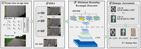
Figure 1. Overall workflow of the proposed methods.

3.1. Transformation of Front View to Top View

Due to the camera’s tilted angle during capturing, the distant part of the road marking is occluded by the foreground, and parallel edges appear to intersect in the image, resulting in compression and deformation of the distant road marking. This deformation not only affects the integrity of the road marking but also reduces the accuracy of damage detection. Therefore, to accurately obtain complete information about the road marking and improve the damage detection accuracy, it is necessary to transform the front view image into a top-down view [42].

The transformation from the front view to the top-down view requires estimating a 3 × 3 homography matrix. To achieve this, four corresponding coordinate points must be identified in both the front and top-down views. It is essential to ensure that the coordinate points in the front view, after being transformed by the homography matrix, accurately correspond to the coordinate points in the top-down view. Figure 2 further illustrates the positional relationship between the four coordinate points in the front view and those in the top-down view. The homography matrix calculation is shown in Equations (1) and (2).

$$\left[\begin{array}{l}{x}^{\prime }\hfill \\ y^{\prime }\hfill \\ 1\hfill \end{array}\right]=H\cdot \left[\begin{array}{l}x\hfill \\ y\hfill \\ 1\hfill \end{array}\right]$$

(1)

where $(x^{\prime },y^{\prime })$ and $(x,y)$ are denoted as the corresponding coordinate points in the top and front views, respectively. $H$ is the homograph matrix of $3\times 3$ of the form:

$$H=\left[\begin{array}{lll}{h}_{11}\hfill & h_{12}\hfill & h_{13}\hfill \\ h_{21}\hfill & h_{22}\hfill & h_{23}\hfill \\ h_{31}\hfill & h_{32}\hfill & h_{33}\hfill \end{array}\right]$$

(2)

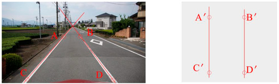
Figure 2. Position of the four coordinate points in the front view in relation to the coordinate points in the top view.

Once the homograph matrix is obtained, any pixel in the front view can be mapped to its corresponding pixel in the top-down view. Therefore, the accurate selection of point coordinates before and after perspective transformation is crucial for estimating the homograph matrix.

Prior to perspective transformation, four coordinates must be selected from the lane lines through lane line fitting. To accomplish this, the semantic segmentation model DeepLabv3 [43] is first employed to extract pixel-level mask values of the lane lines, precisely identifying the positions of each pixel within the lane lines. Based on the extracted mask values, all pixel coordinates of the lane line or lane boundary are collected. These coordinates are fitted using the least squares method to generate a mathematical representation of the lane line. The detailed fitting process is illustrated in Equations (3) and (4).

$$f(x)=Kx+b$$

(3)

$$\underset{\min }{Loss}={{\displaystyle \sum _{i=1}^n(y_i-f(x))}}^2$$

(4)

Equation (4) describes the fitted straight line model, where K is the slope and b denotes the intercept. By minimizing the cost function in this formula, the optimal parameters K, b of the straight line can be obtained, making the fitting more accurate. $y_i$ represents the true value, and $f(x)$ represents the predicted value.

The relative positions of the four coordinate points before and after the perspective transformation are shown in Figure 3.

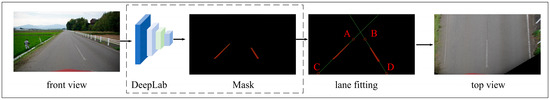
Figure 3. Correspondence of coordinates before and after perspective transformation.

In the transformation process, we assume that the two coordinate points at the bottom before and after the perspective transformation correspond equally, i.e., $\left(x_c,y_c\right)=\left(x_{c^{\prime }},y_{c^{\prime }}\right)$ and $\left(x_D,y_D\right)=\left(x_{D^{\prime }},y_{D^{\prime }}\right)$, and at the same time, the vertical coordinates of A and B take the value of $(height-1100)$, where height is expressed as the height of the picture. Then, the remaining two coordinate points after the transformation can be expressed as shown in Equations (5) and (6).

$$\left(x_{A^{\prime }},y_{A^{\prime }}\right)=\left(x_c,0\right)$$

(5)

$$\left(x_{B^{\prime }},y_{B^{\prime }}\right)=\left(x_D,0\right)$$

(6)

After obtaining the corresponding coordinate points before and after the perspective transformation, the homology matrix can be calculated according to Equation (2). Through this homology matrix, any pixel point in the front view can be accurately mapped to the top view, thus realizing the geometric transformation of the perspective.

3.2. Establishing a Mathematical Model Between a Rectangular Box and a Marked Line

Accurately obtaining the road marking area before and after damage is a critical step in quantifying the damage degree. Currently, mainstream evaluation methods rely on semantic segmentation techniques, which estimate the original area by identifying the marking region. However, when road markings are severely damaged, the lack of sufficient pixel information as feature guidance hinders semantic segmentation methods from accurately reconstructing the original boundaries of the markings, resulting in significant estimation errors in the area.

In real-world environments, road markings of the same type typically exhibit consistent shapes and areas, implying that their corresponding minimum bounding rectangles should theoretically maintain similar dimensions and areas. Leveraging this characteristic, this study proposes a road marking damage assessment method based on the minimum bounding rectangle. By establishing a mathematical mapping relationship between the road marking and its minimum bounding rectangle, the original area of the road marking can be indirectly inferred without relying on complete pixel information, thereby enabling the quantification of the damage degree. To establish the mathematical relationship between the road marking and its minimum bounding rectangle, it is essential to obtain the minimum bounding rectangle of the marking and the corresponding complete road marking area.

As shown in Figure 4, to establish the relationship between the road marking and its minimum enclosing rectangle, we first manually label each pixel of the marking on the original image to obtain the corresponding mask values. After obtaining the mask values, we use OpenCV [44] to find the minimum enclosing rectangle on the mask. The complete road marking area can then be obtained by counting the number of mask values within the enclosing rectangle.

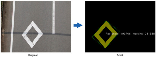
Figure 4. Establish the relationship between the road marking and its minimum enclosing rectangle.

The proposed estimation method based on the minimum enclosing rectangle does not rely on the completeness of the road marking, ensuring high estimation accuracy even in the case of severe damage. Moreover, this method significantly reduces the dependence on the original marking data, making it robust and practical even in scenarios with missing data or complex marking shapes.

3.3. Broken Marker Data Augmentation Method (BMA)

Certain road markings are confined to specific road sections, leading to a limited number of samples. Moreover, the primary focus of this study is to accurately assess the specific degree of damage in road markings. Therefore, during the detection process, special emphasis is placed on precisely identifying severely damaged marking areas to ensure accurate localization and facilitate effective repair of these regions.

Simultaneously, we observed that damaged road markings tend to blend with the color of the road surface. Based on this observation, we propose the BMA data augmentation method. This method randomly overlays road surface color pixels onto the road markings to simulate varying degrees of damage. During this process, no redundant background information is introduced, ensuring that the augmented marking images closely align with the feature distribution of real-world scenarios. The image enhancement process is illustrated in Figure 5, and the corresponding mathematical formulations are provided in Equations (7)–(10).

$$p_{max}=\arg {\max }_p\left({\displaystyle \sum _{(x,y)}\mathbb{I}}(I(x,y)=p)\right)$$

(7)

$$N_{fill}={\displaystyle \frac{r}{100}}\times \mathrm{Area}(R)$$

(8)

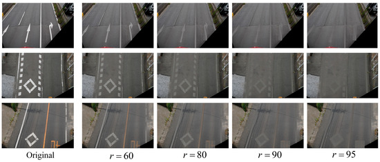
Figure 5. Augmented pavement markings with different levels of damage.

In Equation (7), I(x,y) represents the pixel value of the image at the pixel coordinates (x,y). I(.) is the indicator function, which takes the value of 1 when the condition is true and 0 otherwise. P refers to the possible range of pixel values.

In Equation (8), Area (R) represents the area of the rotated rectangle. Here, r∈{60,80,90,95} denotes the fill percentage within the rotated rectangle R, and $N_{fill}$ represents the total number of filled pixels.

$$S_{flii}=\left\{(x,y)|(x,y)\in R,\left|S_{flii}\right|=N_{flii}\}\right.$$

(9)

$$I^{\prime }(x,y)=\left\{\begin{array}{ll}{p}_{max},\hfill & if(x,y)\in S_{fill};\hfill \\ I(x,y),\hfill & or\hfill \end{array}\right.$$

(10)

In Equation (9), a set of $N_{fill}$ pixel coordinates is randomly selected from the rotated rectangle R for filling. $N_{fill}$ represents the set of selected coordinates. I′ denotes the updated pixel values after the filling process. Algorithm 1 presents the pseudo-code of the proposed method. In Equation (10) $S_{fill}$ denotes the set of coordinates of randomly filled background pixel points. $(x,y)\in R$ means that only the pixel points currently belonging to the rotating rectangular box R are considered. In Equation (17), $I(x,y)$ denotes the pixel value of the original image at $(x,y)$.

Algorithm 1 Pseudo-code of the proposed method BMA. Damaged road marking data augmentation

Input: Input a picture and the rotated label file that corresponds to it.

Output: Updating a BMA-processed image

1: Counts the values of the most frequently occurring pixels in an image in Equation (7). 2: Calculate the number of filled pixel points in Equation (8). 3: Randomly selects the pixel point locations to be filled in Equation (9). 4: Fills the most frequent pixel values to the specified position in Equation (10). 5: End

3.4. Improved Rotating Object Detection Based on YOLOv8

In this study, we propose a method to estimate the intact area of road markings by establishing a mathematical relationship between the markings and their corresponding minimum bounding rectangles. Building upon the YOLOv8 network, we introduce an additional angle prediction branch in the detection head to enable oriented object detection. Additionally, we implement corresponding modifications to other components of the network to improve its adaptability for road marking detection. Figure 6 illustrates the network architecture before and after the modifications.

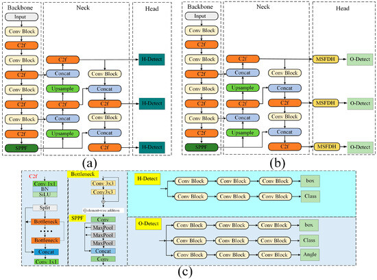
Figure 6. Diagram of YOLOv8 and the modified network structure. (a) Original network; (b) proposed modified network; (c) network module specific components. H-Detect denotes horizontal detection heads, while O-Detect denotes rotational detection heads.

MSFDH: Multi-scale features are essential for road marking detection, as they provide global contextual information and a wider field of view, thereby enhancing the accuracy and consistency of detecting severely damaged markings. Even when parts of the markings are missing or blurred, multi-scale features effectively guide the extension and connection of markings, thereby reducing misdetections. Furthermore, their adaptability to environmental variations, such as lighting changes, occlusions, and weather conditions, significantly improves the robustness and reliability of detection.

Based on this, we propose an MSFDH for road marking detection. MSFDH adopts a multi-branch parallel structure, where different scales of convolutional operations are applied within the same feature map to extract features with various receptive fields. This helps the model better capture pixel relationships and prevents information loss during feature sampling.

Figure 7 illustrates the detailed structure of the proposed MSFDH. The MSFDH structure consists of four parallel branches and a residual branch. The main branches include convolutional modules with kernel sizes of 1 × 1, 3 × 3, 5 × 5, and 7 × 7, while the residual branch consists of a single 1 × 1 convolution module. Notably, each block incorporates a convolutional layer, batch normalization, and a SiLU activation function.

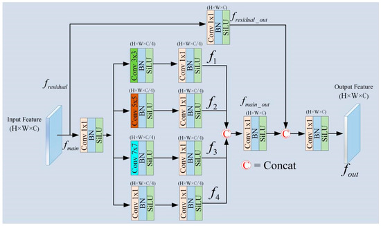
Figure 7. Detailed structure of MSFDH. H and W represent the image size, and C represents the number of channels.

The detailed extraction process of MSFDH features is as follows. Firstly, the feature map with input size H × W × C is divided into the residual branch and main branch. In the main branch, a 1 × 1 convolution is first applied to keep the feature map size constant (Equation (11)). Subsequently, the feature map of the main branch is divided into four sub-branches: the first branch uses only a 1 × 1 convolution for feature extraction; the second branch uses a 3 × 3 convolution followed by a 1 × 1 convolution; and the third and fourth branches use 5 × 5 and 7 × 7 convolutions, respectively, with each convolution operation followed by a 1 × 1 convolution, to integrate the channel information and enhance the model’s ability to understand the multi-channel features. understanding of multi-channel features. At this time, the size of the four branches is H × W × C. In the residual branch, only a 1 × 1 convolution is used for feature extraction, and then the features of the main branch and the residual branch are spliced in the direction of the channel, and the size of the feature map is H × W × 2C. In order to obtain the original size of the feature map, the 1 × 1 convolution is used for the downscaling, so that the final output of the MSFDH is H × W × C, as shown in Equations (11)–(13), and the final output of the MSFDH is H × W × C, which is shown in Equation (13).

$$f_{residual\_out}=\partial (con{v}_{1\times 1}(f_{residual}))$$

(11)

$$f_{main\_out}=\partial (con{v}_{1\times 1}(cat(f_1,f_2,f_3,f_4))$$

(12)

$$f_{main\_out}=\partial (con{v}_{1\times 1}(cat(f_{main\_out},f_{residual\_out}))$$

(13)

where $\partial (•)$ denotes BN and SiLU operations, $conv(•)$ denotes convolution operation, and $cat(•)$ denotes channel splicing.

4. Experimental Verification and Analysis

This section begins by introducing the evaluation metrics for the model, along with the training environment and parameter configurations. Subsequently, the data collection process and the labeling methodology employed in this study are described in detail. For experimental validation, we first establish a mathematical relationship between the intact road marking area and its corresponding minimum bounding rectangle. Next, the performance of the improved rotated object detection method is evaluated in detecting road markings with varying degrees of damage. Ablation studies are conducted to analyze the contributions of individual components of the proposed method, further validating its effectiveness. Finally, the performance of the proposed pavement damage degree detection method is tested on pavement markings of various types and damage degrees.

4.1. Model Evaluation Indicators and Experimental Setting

For better evaluation of deep learning models, the paper uses the most common evaluation metrics including average precision (AP), recall (R), and total average precision (mAP).

$$\mathrm{R}={\displaystyle \frac{TP}{TP+FN}}$$

(14)

$$AP={\displaystyle {\int }_0^{1}p}(r)dr$$

(15)

$$mAP={\displaystyle \frac{1}{N}}{\displaystyle \sum _{i=1}^{N}A{P}_i}$$

(16)

where TP, FP, and FN denote the number of true positives, false positives, and false negatives, respectively. $p(r)$ denotes the precision as a function of the rate of checking completeness, and N denotes the number of target categories detected.

In establishing the mathematical relationship between the area of a pavement marking when it is complete and the corresponding minimum outer rectangle, we used the Pearson correlation coefficient (r), the coefficient of determination (R2), and the mean absolute error (MAE).

$$r={\displaystyle \frac{{\displaystyle \sum \left(x_i-\overline{x}\right)}\left(y_i-\overline{y}\right)}{\sqrt{{\displaystyle \sum {\left(x_i-\overline{x}\right)}^2}{\displaystyle \sum {\left(y_i-\overline{y}\right)}^2}}}}$$

(17)

$$R^2=1-{\displaystyle \frac{{\displaystyle \sum {\left(y_i-{\widehat{y}}_i\right)}^2}}{{\displaystyle \sum {\left(y_i-\overline{y}\right)}^2}}}$$

(18)

$$\mathrm{MAE}={\displaystyle \frac{1}{n}}{\displaystyle \sum _{i=1}^n\left|y_i-{\widehat{y}}_i\right|}$$

(19)

In the formulas, $x_i$ represents the independent variable, which is set as the area of the minimum bounding rectangle corresponding to the road marking in this experiment. $y_i$ represents the dependent variable, defined as the actual road marking area when intact.

The Pearson correlation coefficient ranges from [−1, 1], where r > 0 indicates a positive correlation, r < 0 indicates a negative correlation, and values closer to 1 indicate a stronger positive correlation. In Equation (18), ${\widehat{y}}_i$ denotes the predicted value obtained from the regression model for the i-th dependent variable. The coefficient of determination (R²) ranges from [0, 1], where R² = 1 indicates that the model fully explains the variation in the dependent variable, while R2 = 0 indicates no explanatory power. Additionally, the MAE is used to assess model bias, with lower values closer to zero indicating better performance.

All experimental models in this paper were run on a Windows 11 computer with an Intel(R)Core(TM), i9-14900K, 3.20GHz processor and a 24G-sized 4090 graphics card. All code was run in Python within the pytorch framework. Table 1 shows a more specific model runtime environment configuration.

Table 1. Experimental environment and hyperparameter settings.

Experimental Environment		Model Hyperparameter Settings
GPU	4090(24 G)	Image Size	640 × 640
CPU	Intel, i9-14900K, 3.20 GHz	Epochs	200
Python	3.8.18	Batch Size	4
Pytorch	2.1.1	Momentum	0.937
Cuda	11.8	Initial learning rate	0.01
systems	Windows 11	Final learning rate	0.01

4.2. Dataset

In this study, a comprehensive road marking dataset was constructed to validate the proposed method and facilitate deep learning model training and testing. The dataset was collected using a Sony α6500 camera mounted on the roof of a vehicle, as illustrated in Figure 8. The images were captured at two resolutions: 3008 × 1688 and 4240 × 2400. The dataset comprises 3200 images, all captured from real-world road scenes. To ensure image clarity, all photographs were captured under clear weather conditions. The dataset exhibits significant diversity, encompassing various road conditions, marking types (including arrow indicators, zebra crossings, lane boundary lines, guide lines, and speed bump markings), and varying degrees of damage. This diversity ensures the dataset’s broad applicability for model training and evaluation.

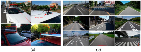
Figure 8. Data acquisition equipment. (a) Data collection and pictures (b) Road markings.

4.3. Data Labeling

In this study, road marking damage detection is primarily based on the mathematical relationship between the area of the minimum bounding rectangle and the intact marking area within it. To accurately obtain the minimum bounding rectangle, OOD is utilized for labeling. The method described in Section 3.2 is applied to determine the minimum bounding rectangle for each marking. Once the minimum rotated rectangle is obtained, its center coordinates (cx, cy), width, height, and rotation angle are recorded in an XML file to generate training labels. This study focuses on detecting seven distinct types of road markings. Therefore, a dataset was constructed for these seven marking types, with the specific categories and label names illustrated in Figure 9. During model training, the dataset was divided into a ratio of 7:2:1 for training, testing, and validation, respectively.

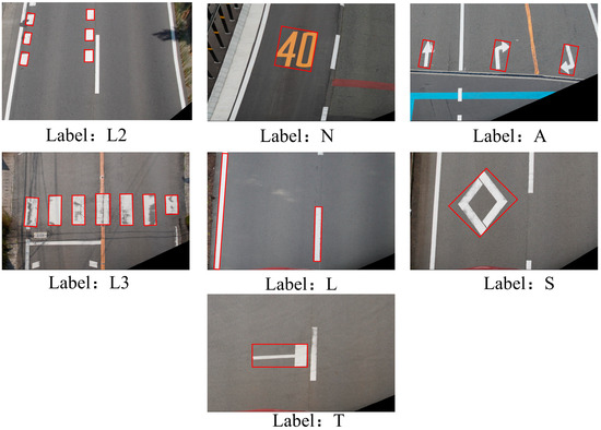
Figure 9. The different types of markers detected and the corresponding labels.

4.4. Experimental Verification

4.4.1. Mathematical Relationship Between a Labeled Line and Its Minimum Outer Rectangle

To accurately establish the mathematical relationship between the intact road marking area and its corresponding minimum bounding rectangle area, this experiment analyzed clear and complete road markings, including typical samples such as directional arrows, zebra crossings, lane edge lines, and speed bumps. The results are illustrated in Figure 10, where the red scatter plot represents the relationship between the minimum bounding rectangle area and the corresponding road marking area. In the figure, the minimum bounding rectangle area is treated as the independent variable (x-axis), while the actual road marking area serves as the dependent variable (y-axis).

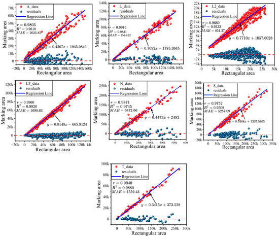
Figure 10. Illustrates the relationship between the area of a pavement marking and the area of its corresponding minimum outer rectangle.

Figure 10 presents a red scatter plot illustrating the distribution trend between the x-axis (minimum bounding rectangle area) and the y-axis (road marking area). The analysis reveals a significant linear relationship between the two, and a linear model was derived through data fitting. The fitting results for seven distinct types of road markings (arrow indication A, zebra crossing L3, lane edge line L, speed bump S, speed limit sign N, speed limit warning L2, and straight-line intersection) indicate that for the detected L, T, S, L3, N, and A road marking types, the Pearson correlation coefficient r exceeds 0.97, and the coefficient of determination R2 exceeds 0.95, demonstrating the high accuracy of the linear model fitting. A very strong linear relationship exists between the two variables. For the L2 road marking type, the Pearson correlation coefficient is r = 0.9660, and the coefficient of determination is R2 = 0.9332. Although slightly lower than the other categories, a strong linear relationship still exists, and the mathematical relationship between them can be accurately represented by a linear model. Additionally, the corresponding residual distribution plot is provided. From the residual distribution, it is evident that the residual points are predominantly concentrated near x = 0, and the residual mean is close to zero, indicating that the model’s predictions closely align with the actual values, with no systematic error. Moreover, the residual distribution does not exhibit any noticeable trend with changes in the independent variable (minimum bounding rectangle area), indicating that the model performs stably across different ranges of the independent variable and that the fitting is effective. Based on this analysis, it can be further confirmed that a significant linear correlation exists between the minimum bounding rectangle area and the road marking area, and the relationship between the two can be accurately represented by a linear model.

4.4.2. Minimum Outer Rectangular Box Detection

(1)

Analysis of experimental results

To validate the performance and advantages of the proposed method over the YOLOv8 series rotated object detection method for damaged road surfaces, a quantitative analysis was performed on our self-built dataset, as presented in Table 2. The proposed method achieved an accuracy of 97.4% on the self-built dataset, representing a 4.5% improvement in mAP50 over the baseline YOLOv8s model. Figure 11 illustrates the loss values and mAP trends during the training process of the proposed method and other models. Compared to other models, the proposed method exhibits faster convergence. Furthermore, the improved model achieves the best detection performance in the mAP50:95 metric. As presented in Table 3, the improved model demonstrates strong robustness and generalization across various IoU thresholds, enabling more precise localization and identification of road markings. This indicates that the proposed method offers a significant advantage in balancing detection accuracy and localization precision. More accurate road marking localization ensures the precise identification of the minimum bounding rectangle, providing a reliable foundation for the subsequent calculation of road marking damage severity.

Table 2. mAP50 performance comparison.

Methods	AP50							mAP50
	L	L2	L3	N	S	A	T
YOLOv8n	0.955	0.972	0.874	0.977	0.889	0.931	0.887	0.927
YOLOv8s	0.96	0.974	0.872	0.975	0.914	0.924	0.881	0.929
YOLOv8m	0.962	0.975	0.879	0.968	0.920	0.939	0.871	0.931
YOLOv8l	0.963	0.977	0.916	0.974	0.946	0.951	0.886	0.945
YOLOv8x	0.963	0.979	0.924	0.978	0.948	0.969	0.907	0.953
ours	0.976	0.985	0.935	0.992	0.993	0.995	0.941	0.974

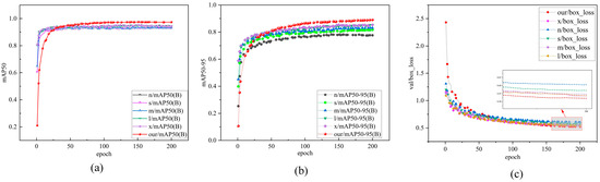
Figure 11. Comparison of training metrics for different models. (a) mAP50. (b) mAP50:95. (c) Training loss.

Table 3. mAP50:95 performance comparison.

Methods	AP50:95							mAP50:95
	L	L2	L3	N	S	A	T
YOLOv8n	0.821	0.869	0.788	0.821	0.722	0.767	0.707	0.784
YOLOv8s	0.854	0.889	0.803	0.843	0.755	0.797	0.761	0.816
YOLOv8m	0.866	0.910	0.814	0.849	0.791	0.838	0.751	0.831
YOLOv8l	0.869	0.912	0.852	0.868	0.843	0.848	0.781	0.853
YOLOv8x	0.86	0.907	0.849	0.873	0.839	0.864	0.907	0.855
ours	0.862	0.903	0.878	0.879	0.957	0.960	0.799	0.891

Additionally, Figure 11 shows the changes in mAP50, mAP50:95, and bounding box loss during training across different models. The results indicate that after 50 training epochs, the proposed method demonstrates significant advantages in detecting the minimum enclosing rectangle for road markings. However, in the early stages of training (especially when the epoch is less than 50), the detection performance of this method is notably lower than that of other methods. This is primarily due to the modified network structure, which includes some reinitialized network layers, resulting in lower metrics in the early training phase. It is worth noting that after 100 training epochs, the bounding box loss of the proposed method significantly converges, exhibiting superior stability and generalization compared to other models.

Figure 12 presents the mixing matrices of different methods, quantifying the model’s prediction errors across categories and clearly showing the correspondence between true labels and predicted results. Analyzing the mixing matrices of different models reveals that the proposed minimum enclosing rectangle-based road marking detection method outperforms all other models. Specifically, the detection accuracy of this method for road marking categories L, L2, L3, N, S, A, and T reaches 0.96, 0.97, 0.89, 0.98, 0.98, 0.99, and 0.87, respectively, all of which are higher than the classification accuracy of other models.

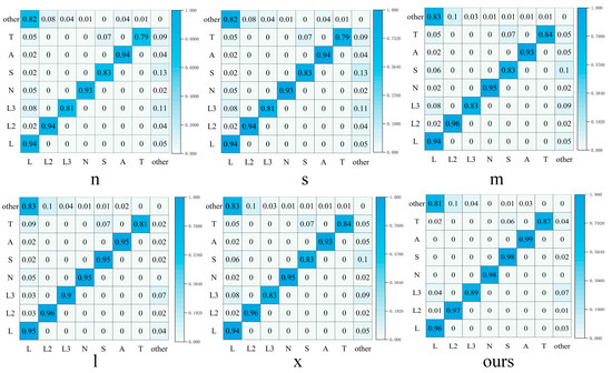
Figure 12. Comparison of mixing matrices of different models.

Table 4 presents a comparative analysis of the proposed method and the YOLOv8 series in terms of detection efficiency, model parameters, and computational complexity. It can be observed that although our method increases the number of parameters from 20.5M to 27.8M and the FLOPs from 24.3G to 29.1G based on the YOLOv8s model, the inference time per image only slightly increases by 0.2 ms. Combined with the experimental results in Table 2 and Table 3, it demonstrates that the proposed method achieves a notable improvement in detection accuracy while maintaining near real-time performance, thus offering a more favorable trade-off between performance and efficiency.

Table 4. Comparative analysis of different models in terms of parameter size, computational complexity, and inference speed.

Methods	Category	Size(M)	FLOPs	Processing Time
YOLOv8	n	5.8	7.1G	3.3 ms
	s	20.5	24.3G	3.3 ms
	m	47.9	69.6G	3.4 ms
	l	81.8	148.9G	3.8 ms
	x	126.4	232.5G	4.5 ms
	ours	27.8	29.1G	3.5 ms

In order to further verify the generalization performance of the proposed method under different detection frameworks, as well as its adaptability and accuracy in oriented target detection tasks, this paper conducts extended experiments on multiple mainstream lightweight target detection models. Specifically, they include modified versions of YOLOv3, YOLOv5, YOLOv6, YOLOv9 and Mobilev3. For these models, we introduce angle regression branches into their original structures to enable them to have the ability to predict the rotated bounding box, thereby realizing the oriented detection of road marking targets. Table 5 shows the comparison results of the detection performance of each model on multiple types of road marking datasets. The comparison mainly revolves around two groups of models: one group is a baseline version that only adds the angle prediction branch on the basis of the original lightweight model, and the other group further introduces the improved module proposed in this paper on this basis. From the experimental results, it can be seen that after introducing the improved method proposed in this paper into each detection model, its detection performance is significantly improved compared with the baseline model that only adds the angle prediction branch. This result shows that the proposed method has good versatility, can stably adapt to lightweight detection frameworks of different structures, and effectively improve the accuracy and robustness of directional target detection.

Table 5. Comparison of mAP50 of different models, w/ indicates that the network structure is modified using the method proposed in this paper.

Methods	AP50							mAP50
	L	L2	L3	N	S	A	T
YOLOv3-tiny	0.913	0.94	0.824	0.986	0.904	0.926	0.896	0.913
w/	0.932	0.955	0.902	0.989	0.989	0.986	0.915	0.952
YOLOv5n	0.953	0.972	0.844	0.991	0.921	0.939	0.836	0.922
w/	0.905	0.965	0.878	0.954	0.987	0.99	0.936	0.945
YOLOv5s	0.959	0.982	0.874	0.973	0.902	0.942	0.89	0.932
w/	0.973	0.985	0.921	0.987	0.991	0.995	0.914	0.966
YOLOv6n	0.947	0.969	0.826	0.974	0.868	0.909	0.854	0.907
w/	0.876	0.976	0.859	0.956	0.964	0.976	0.815	0.917
YOLOv6s	0.951	0.969	0.856	0.993	0.901	0.917	0.884	0.924
w/	0.873	0.974	0.885	0.98	0.972	0.991	0.876	0.936
YOLOv9-tiny	0.96	0.977	0.87	0.989	0.902	0.936	0.849	0.926
w/	0.893	0.984	0.921	0.98	0.992	0.991	0.913	0.953
YOLOv9s	0.963	0.98	0.87	0.983	0.93	0.934	0.899	0.937
w/	0.976	0.985	0.948	0.985	0.987	0.995	0.935	0.973
Mobilev3	0.923	0.945	0.836	0.983	0.924	0.937	0.894	0.921
w/	0.937	0.956	0.902	0.989	0.989	0.983	0.914	0.953
ours	0.976	0.985	0.935	0.992	0.993	0.995	0.941	0.974

(2)

Analysis of ablation experiments

A: BMA ablation experiments

To verify the effectiveness and importance of the proposed data augmentation method in the network structure, this study conducted a validation experiment focusing on evaluating the performance of medium-complexity models. The experiment compared the effects of not applying any data augmentation, applying the Mosaic and Mixup methods, and applying the proposed BMA method. In the BMA experiment, selective augmentation was applied to datasets with relatively fewer samples. The comparison of the training and validation datasets before and after augmentation is shown in Figure 13. Table 6 displays the experimental results of different network structures after adding various data augmentation methods.

Figure 13. Distribution of data before and after enhancement. (a) Data used for training. (b) Data used for validation.

Table 6. Comparison of the effect of different data enhancement methods.

Methods	Mosaic	Mixup	BMA	Map50	Map50:95
YOLOv8n	-	-	-	92.7	78.3
	√	-	-	93.5	79.2
	-	√	-	93.0	79.1
	-	-	√	95.7	86.1
YOLOv8s	-	-	-	92.9	81.6
	√	-	-	94.4	82.3
	-	√	-	93.6	81.8
	-	-	√	97.1	89.0
YOLOv8m	-	-	-	93.1	83.2
	√	-	-	94.1	83.6
	-	√	-	94.0	84.4
	-	-	√	96.8	90.1

In the data augmentation validation experiment, we selected smaller-scale and less complex N, S, and M versions for the comparative experiment, rather than the larger L and X versions. The main reason for this choice is that the N, S, and M models strike a balance between computational efficiency and model size, making them suitable for evaluating the effectiveness of data augmentation methods. In contrast, the L and X models, with their higher model complexity and computational requirements, can extract more detailed features, which may lead to performance improvements that partially stem from the complexity of the network itself. Therefore, selecting the N, S, and M models allows for a more accurate evaluation of the actual effect of data augmentation strategies across different model scales.

The experimental results shown in Table 4 indicate that the proposed BMA data augmentation method significantly improved detection performance. Using the BMA augmentation method in the N model increased the mAP50 and mAP50:95 to 95.7 and 86.1, respectively, achieving a clear performance advantage over the Mosaic and MixUp methods. Additionally, the proposed method also demonstrated strong performance in the S and M models, indicating that the proposed damage data augmentation method can simulate road markings with varying levels of damage. This enhancement improves the model’s ability to perceive features of damaged markings, thereby improving overall performance.

B: MSFDH Ablation Experiment

To further validate the effectiveness and importance of the proposed MSFD in the model, we also conducted a standalone verification experiment for the MSFDH. To assess the proposed method’s effectiveness more comprehensively, we performed experimental comparisons using SE [45], CA [46], and CBAM [47] at the same positions. Table 7 presents the results of these comparative experiments. The evaluation was based on three metrics: mAP50, mAP50:95, and R (Recall).

Table 7. Comparison of model performance by different modules at the same location.

Method	SE	CA	CBAM	MSFDH	Map50	Map50:95	R
YOLOv8s	-	-	-	-	92.9	81.6	89.5
	√	-	-	-	93.1	81.7	90.4
	-	√	-	-	92.9	81.5	89.7
	-	-	√	-	92.5	80.9	86.9
	-	-	-	√	93.5	81.9	90.1

Table 5 presents the detailed experimental results. When no modules were added to the detection head, the model’s mAP50, mAP50:95, and R values were 92.9%, 81.6%, and 89.5%, respectively. After incorporating the SE attention module, there was a slight increase in mAP50 and mAP50:95, with values rising to 93.1% and 81.7%, while R showed a noticeable improvement, increasing to 90.4%. This indicates that the SE attention module enhances feature representation and improves recall in the damaged road marking scenario. When the CA attention module was introduced, there was little change in mAP50 and mAP50:95, with values remaining at 92.9% and 81.5%, while R slightly increased to 89.7%. However, when the CBAM attention module was applied, all three performance metrics showed a significant decline, suggesting that CBAM is less suitable for this specific task. In contrast, after using the proposed MSFDH detection head, the model’s performance showed significant improvement, with mAP50, mAP50:95, and R reaching 93.5%, 81.9%, and 90.1%, respectively. This demonstrates that the proposed MSFDH detection head is better suited for the current task scenario and further confirms its ability to extract feature information with different receptive fields within the same feature map, enabling the model to better understand pixel relationships.

C: MSFDH and BMA ablation experiments

Table 8 presents the results of the ablation experiments on the baseline model, focusing on the impact of the BMA and the proposed MSFDH modules on model detection accuracy. The baseline model (without BMA and MSFDH) achieved mAP50 and mAP50:95 values of 92.9% and 81.6%, respectively. When the BMA module was introduced alone, mAP50 and mAP50:95 significantly improved to 97.1% and 89.0%, demonstrating that BMA effectively enhances detection performance. Introducing the MSFDH module alone resulted in mAP50 and mAP50:95 values of 93.5% and 81.9%, indicating that MSFDH also positively contributes to detection accuracy. When both the BMA and MSFDH modules were introduced simultaneously, mAP50 further increased to 97.4%, and mAP50:95 reached 89.1%, suggesting that MSFDH can further optimize target detection performance on top of the improvements made by BMA. Overall, BMA has a more significant impact on improving detection accuracy, while the inclusion of MSFDH further enhances detection capabilities and may offer additional structural optimization advantages.

Table 8. Effect of BMA and MSFDH modules on detection performance.

Method	BMA	MSFDH	Map50	Map50:95	R
YOLOv8s	-	-	92.9	81.6	89.5
	√	-	97.1	89.0	95.6
	-	√	93.5	81.9	90.1
	√	√	97.4	89.1	94.1

Additionally, to more clearly present the performance metrics of the proposed method, Figure 14 illustrates the mAP50 and mAP50:95 trends during the training process for the baseline model, models with only BMA or MSFDH, and the model with both BMA and MSFDH. From the figure, it can be observed that both BMA and MSFDH significantly outperform the baseline model when introduced individually. However, the model with both BMA and MSFDH performs the best, further validating the synergistic optimization effect of the two modules.

Figure 14. Training process of BMA and MSFDH module.

Figure 15 shows the detection results of the proposed minimum bounding rectangle method when applied to different types of road markings with varying levels of damage. The results indicate that for intact road markings with clear edges, the method is able to reliably obtain their minimum bounding rectangle. Even in cases of severe damage with discontinuous textures, the proposed method can still accurately determine the minimum bounding rectangle while maintaining a high confidence level. This result further validates the robustness and accuracy of the method in complex scenarios.

Figure 15. Minimum bounding rectangle detection of pavement markings with different levels of damage.

(3)

Experimental detection of the degree of damage

The assessment of road marking damage requires knowledge of the area before and after damage. For the pre-damage area, we use the proposed method to evaluate the area of the marking before damage by detecting the minimum bounding rectangle. For the post-damage area, we perform pixel counting within the detected minimum bounding rectangle by setting a threshold, where the actual marking color is typically yellow or white. The formula for calculating the damage rate is given in Equation (20).

$$Rate={\displaystyle \frac{|S_2-S_1|}{S_2}}\times 100\%$$

(20)

In Equation (20), S2 represents the estimated marking area using the minimum bounding rectangle (the area of the marking when intact). The area estimation formula for different types of markings is given in Equation (21). Here, Class denotes the detected marking category, and there exists a different mathematical relationship between the minimum bounding rectangle area and the actual marking area for each category. The variable x represents the area of the detected minimum bounding rectangle. In Equation (20), S1 represents the total area of white (or yellow) pixels within the minimum bounding rectangle (i.e., the area after marking damage). The calculation of S1 is as follows: within the current minimum bounding rectangle, a pixel intensity threshold is set. Pixels with intensity values greater than the threshold are classified as belonging to the white (or yellow) marking region, and their total area is then computed.

$$S_2=\left\{\begin{array}{cc}0.7692x+1785.3645\hfill & \hfill class=L\\ 0.5488x+1307.5465\hfill & \hfill class=S\\ 0.3415x+373.5280\hfill & \hfill class=T\\ 0.7710x+1057.6028\hfill & \hfill class=L2\\ 0.4473x+2492.2043\hfill & \hfill class=N\\ 0.4267x+1945.0846\hfill & \hfill class=A\\ 0.9148x-665.9124\hfill & \hfill class=L3\end{array}\right.$$

(21)

Figure 16 illustrates the degree of damage detected by the proposed method for pavement markings in relatively intact conditions. In the figure, each rotated rectangular box corresponds to a category label. Equation (21) is used to calculate S2 based on the category label, and the rotated box is traversed to calculate S1. Finally, Equation (20) is applied to determine the final damage rate of the marking. The percentage following each label in Figure 16 indicates the degree of damage of the labeled marking at that location. From the figure, it is evident that for various types of pavement markings with different degrees of damage, the proposed method can accurately calculate their specific damage values.

Figure 16. Detection of the degree of damage of different types of pavement markings.

It can be observed in the figure that the theoretical breakage rate should be 0 for the breakage markers of category ‘L’, but the experimental results show slightly higher values than 0 for this category (0.93%, 5.20%, 4.94%, 2.83%, etc.). Despite the deviation in values, the overall value is close to 0 and the margin of error is within the acceptable range. The main reason for this deviation is that the simple judgment method based on pixel thresholds was used to calculate the indicator S1, which is easily affected by changes in lighting conditions, leading to a small calculation result, which in turn introduces a certain degree of error.

For the markers with category ‘N’, the main source of calculation error is that the data labeling process unifies numerical markers such as ‘40’, ‘50’, and ‘30’. ‘30’, ‘40’, ‘50’ and other digital markers are uniformly classified as “N”, and when calculating the mathematical relationship between the minimum external rotating rectangular box and the area of the internal markers, the actual area of different digital markers varies, resulting in a certain degree of bias in the calculation results. Similarly, for markings with category ‘A’, since the arrows indicating different driving directions (e.g., straight ahead, left turn, right turn) are uniformly classified as ‘A’ in the data labeling, there are significant differences in their morphological characteristics, so errors are also inevitably introduced in the establishment of mathematical relationships to calculate the breakage rate. Therefore, when establishing the mathematical relationship to calculate the breakage rate, errors are inevitably introduced. However, from the overall results, the method proposed in this paper can still accurately reflect the degree of damage of different types of markings, which proves the effectiveness of the method in the task of detecting the damage of pavement markings.

5. Methodological Limitations and Future Research Directions

The evaluation method proposed in this paper efficiently quantifies road marking quality by constructing a mathematical mapping between the area of road markings and their minimum bounding rectangle. However, this approach still has limitations in certain complex scenarios. For example, for lane markings with significant geometric curvature (category L), a single rectangle cannot accurately depict their true shape, potentially introducing significant evaluation errors. Furthermore, when the image does not fully cover the entire length of the marking, the accuracy of the evaluation results is also affected. To address these issues, future research could focus on the following three directions: First, curved road markings could be segmented and modeled using multi-rectangle fitting to improve the accuracy of morphological representation; second, a road marking integrity detection module could be incorporated into the evaluation framework to quantify damage only when the marking is completely captured, enhancing robustness; finally, road marking categories could be further refined. For example, corresponding mathematical mapping models could be established for speed limit signs in category N (e.g., “40” and “50”), enabling more targeted quality assessment.

6. Summary and Discussion

In this study, a novel method for detecting the degree of damage to pavement markings is proposed. Specifically, a mathematical model is established between different types of pavement markings and their minimum bounding rectangles based on the top-view perspective, enabling the assessment of the intact area of internal markings through the detection of these bounding rectangles. Additionally, to accurately determine the minimum bounding rectangle of the markings, several improvement methods are proposed to enhance the accuracy and robustness of detection. The experimental results demonstrate that in the detection of minimum bounding rectangles, the proposed improvement methods achieve the best performance on the small model, providing a foundation for the subsequent accurate determination of pavement marking damage degree. Furthermore, the experiments also demonstrate that the proposed pavement marking damage detection method can accurately determine the damage degree for various types of markings, further validating the correctness and reliability of the proposed method. The method proposed in this paper is simple and effective, and can accurately obtain the degree of damage to the marking, providing accurate data support for timely maintenance and repair of pavement marking.

In future research, we plan to further refine the categories of markings and establish more precise mathematical models for different types of markings to enhance the accuracy of damage degree assessment. Additionally, when calculating S, the integration of image segmentation technology is considered to further improve detection accuracy and enhance the practical application value of this method in road traffic safety.

References

- Chen, T.; Dai, J.; Dong, B.; Zhang, T.; Xu, W.; Wang, Z. Road marking defect detection based on CFG_SI_YOLO network. Digit. Signal Process. 2024, 153, 104614. [Google Scholar] [CrossRef]
- Zou, Q.; Jiang, H.; Dai, Q.; Yue, Y.; Chen, L.; Wang, Q. Robust Lane Detection From Continuous Driving Scenes Using Deep Neural Networks. IEEE Trans. Veh. Technol. 2019, 69, 41–54. [Google Scholar] [CrossRef]
- Jin, D.; Park, W.; Jeong, S.-G.; Kwon, H.; Kim, C.-S. Eigenlanes: Data-Driven Lane Descriptors for Structurally Diverse Lanes. In Proceedings of the 2022 IEEE/CVF Conference on Computer Vision and Pattern Recognition (CVPR), New Orleans, LA, USA, 18–24 June 2022; pp. 17142–17150. [Google Scholar]
- Zhang, Y.; Lu, Z.; Ma, D.; Xue, J.-H.; Liao, Q. Ripple-GAN: Lane Line Detection With Ripple Lane Line Detection Network and Wasserstein GAN. IEEE Trans. Intell. Transp. Syst. 2020, 22, 1532–1542. [Google Scholar] [CrossRef]
- Yu, Y.; Li, Y.; Liu, C.; Wang, J.; Yu, C.; Jiang, X.; Wang, L.; Liu, Z.; Zhang, Y. MarkCapsNet: Road Marking Extraction From Aerial Images Using Self-Attention-Guided Capsule Network. IEEE Geosci. Remote Sens. Lett. 2021, 19, 1–5. [Google Scholar] [CrossRef]
- Cao, J.; Song, C.; Song, S.; Xiao, F.; Peng, S. Lane Detection Algorithm for Intelligent Vehicles in Complex Road Conditions and Dynamic Environments. Sensors 2019, 19, 3166. [Google Scholar] [CrossRef]
- Andreev, S.; Petrov, V.; Huang, K.; Lema, M.A.; Dohler, M. Dense Moving Fog for Intelligent IoT: Key Challenges and Opportunities. IEEE Commun. Mag. 2019, 57, 34–41. [Google Scholar] [CrossRef]
- Dong, Z.; Zhang, H.; Zhang, A.A.; Liu, Y.; Lin, Z.; He, A.; Ai, C. Intelligent pixel-level pavement marking detection using 2D laser pavement images. Measurement 2023, 219, 113269. [Google Scholar] [CrossRef]
- Chimba, D.; Kidando, E.; Onyango, M. Evaluating the Service Life of Thermoplastic Pavement Markings: Stochastic Approach. J. Transp. Eng. Part B Pavements 2018, 144, 04018029. [Google Scholar] [CrossRef]
- Pike, A.M.; Whitney, J.; Hedblom, T.; Clear, S. How Might Wet Retroreflective Pavement Markings Enable More Robust Machine Vision? Transp. Res. Rec. J. Transp. Res. Board 2019, 2673, 361–366. [Google Scholar] [CrossRef]
- Chen, T.; Chen, Z.; Shi, Q.; Huang, X. Road marking detection and classification using machine learning algorithms. In Proceedings of the IEEE Intelligent Vehicles Symposium, Seoul, Republic of Korea, 28 June–1 July 2015; pp. 617–621. [Google Scholar] [CrossRef]
- Mammeri, A.; Boukerche, A.; Lu, G. Lane detection and tracking system based on the MSER algorithm, hough transform and kalman filter. In Proceedings of the MSWiM’14: 17th ACM International Conference on Modeling, Analysis and Simulation of Wireless and Mobile Systems, Montreal, QC, Canada, 21 September 2014; pp. 259–266. [Google Scholar]
- Ye, Y.Y.; Chen, H.J.; Hao, X.L. Lane marking detection based on waveform analysis and CNN. In Proceedings of the Second International Workshop on Pattern Recognition, Singapore, 19 June 2017; pp. 211–215. [Google Scholar]
- Ying, Z.; Li, G. Robust lane marking detection using boundary-based inverse perspective mapping. In Proceedings of the 2016 IEEE International Conference on Acoustics, Speech and Signal Processing (ICASSP), Shanghai, China, 20–25 March 2016; pp. 1921–1925. [Google Scholar]
- Zheng, B.; Tian, B.; Duan, J.; Gao, D. Automatic detection technique of preceding lane and vehicle. In Proceedings of the 2008 IEEE International Conference on Automation and Logistics (ICAL), Qingdao, China, 1–3 September; pp. 1370–1375.
- Zhou, S.; Jiang, Y.; Xi, J.; Gong, J.; Xiong, G.; Chen, H. A novel lane detection based on geometrical model and gabor filter. In Proceedings of the 2010 IEEE Intelligent Vehicles Symposium, La Jolla, CA, USA, 21–24 June 2010; pp. 59–64. [Google Scholar]
- Al-Huda, Z.; Peng, B.; Algburi, R.N.A.; Al-Antari, M.A.; Al-Jarazi, R.; Zhai, D. A hybrid deep learning pavement crack semantic segmentation. Eng. Appl. Artif. Intell. 2023, 122, 106142. [Google Scholar] [CrossRef]
- Wei, C.; Li, S.; Wu, K.; Zhang, Z.; Wang, Y. Damage inspection for road markings based on images with hierarchical semantic segmentation strategy and dynamic homography estimation. Autom. Constr. 2021, 131, 103876. [Google Scholar] [CrossRef]
- Jang, W.; Hyun, J.; An, J.; Cho, M.; Kim, E. A Lane-Level Road Marking Map Using a Monocular Camera. IEEE/CAA J. Autom. Sin. 2021, 9, 187–204. [Google Scholar] [CrossRef]
- Sun, L.; Yang, Y.; Yang, Z.; Zhou, G.; Li, L. DUCTNet: An Effective Road Crack Segmentation Method in UAV Remote Sensing Images Under Complex Scenes. IEEE Trans. Intell. Transp. Syst. 2024, 25, 12682–12695. [Google Scholar] [CrossRef]
- Kong, W.; Zhong, T.; Mai, X.; Zhang, S.; Chen, M.; Lv, G. Automatic Detection and Assessment of Pavement Marking Defects with Street View Imagery at the City Scale. Remote Sens. 2022, 14, 4037. [Google Scholar] [CrossRef]
- Wu, P.; Wu, J.; Xie, L. Pavement distress detection based on improved feature fusion network. Measurement 2024, 236, 115119. [Google Scholar] [CrossRef]
- Li, J.; Yuan, C.; Wang, X. Real-time instance-level detection of asphalt pavement distress combining space-to-depth (SPD) YOLO and omni-scale network (OSNet). Autom. Constr. 2023, 155, 105062. [Google Scholar] [CrossRef]
- Iparraguirre, O.; Iturbe-Olleta, N.; Brazalez, A.; Borro, D. Road Marking Damage Detection Based on Deep Learning for Infrastructure Evaluation in Emerging Autonomous Driving. IEEE Trans. Intell. Transp. Syst. 2022, 23, 22378–22385. [Google Scholar] [CrossRef]
- Hoang, T.M.; Nguyen, P.H.; Truong, N.Q.; Lee, Y.W.; Park, K.R. Deep RetinaNet-Based Detection and Classification of Road Markings by Visible Light Camera Sensors. Sensors 2019, 19, 281. [Google Scholar] [CrossRef]
- Azmi, N.H.; Sophian, A.; Bawono, A.A. Deep-learning-based detection of missing road lane markings using YOLOv5 algorithm. IOP Conf. Ser. Mater. Sci. Eng. 2022, 1244, 012021. [Google Scholar]
- Wu, J.; Liu, W.; Maruyama, Y. Street View Image-Based Road Marking Inspection System Using Computer Vision and Deep Learning Techniques. Sensors 2024, 24, 7724. [Google Scholar] [CrossRef]
- Wang, J.; Zeng, X.; Wang, Y.; Ren, X.; Wang, D.; Qu, W.; Liao, X.; Pan, P. A Multi-Level Adaptive Lightweight Net for Damaged Road Marking Detection Based on Knowledge Distillation. Remote Sens. 2024, 16, 2593. [Google Scholar] [CrossRef]
- Jocher, G.; Chaurasia, A. Ultralytics YOLO. Available online: https://github.com/ultralytics/ultralytics (accessed on 3 June 2024).
- Zhang, H.; Wang, Y.; Dayoub, F.; Sunderhauf, N. Varifocalnet: An iou-aware dense object detector. In Proceedings of the IEEE/CVF Conference on Computer Vision and Pattern Recognition, Nashville, TN, USA, 20–25 June; pp. 8514–8523.
- Lin, H.; Liu, J.; Zhi, N. Yolov7-DROT: Rotation Mechanism Based Infrared Object Fault Detection for Substation Isolator. IEEE Trans. Power Deliv. 2024, 40, 50–61. [Google Scholar] [CrossRef]
- Zou, H.; Wang, Z. An enhanced object detection network for ship target detection in SAR images. J. Supercomput. 2024, 80, 17377–17399. [Google Scholar] [CrossRef]
- Zhang, C.; Xiong, B.; Li, X.; Zhang, J.; Kuang, G. Learning Higher Quality Rotation Invariance Features for Multioriented Object Detection in Remote Sensing Images. IEEE J. Sel. Top. Appl. Earth Obs. Remote Sens. 2021, 14, 5842–5853. [Google Scholar] [CrossRef]
- Tan, Z.; Jiang, Z.; Yuan, Z.; Zhang, H. OPODet: Toward Open World Potential Oriented Object Detection in Remote Sensing Images. IEEE Trans. Geosci. Remote Sens. 2024, 62, 1–13. [Google Scholar] [CrossRef]
- Zhang, H.; Cisse, M.; Dauphin, Y.N.; Lopez-Paz, D. mixup: Beyond empirical risk minimization. arXiv 2017, arXiv:1710.09412. [Google Scholar]
- Bochkovskiy, A.; Wang, C.Y.; Liao, H.Y.M. Yolov4: Optimal speed and accuracy of object detection. arXiv 2020, arXiv:2004.10934. [Google Scholar] [CrossRef]
- Lin, T.Y.; Dollár, P.; Girshick, R.; He, K.; Hariharan, B.; Belongie, S. Feature pyramid networks for object detection. In Proceedings of the IEEE Conference on Computer Vision and Pattern Recognition, Honolulu, HI, USA, 21–26 July 2017. [Google Scholar] [CrossRef]
- Liu, S.; Qi, L.; Qin, H.; Shi, J.; Jia, J. Path Aggregation Network for Instance Segmentation. In Proceedings of the 2018, IEEE/CVF Conference on Computer Vision and Pattern Recognition (CVPR), Salt Lake City, UT, USA, 18–23 June 2018. [Google Scholar] [CrossRef]
- Tan, M.; Pang, R.; Le, Q.V. EfficientDet: Scalable and efficient object detection. In Proceedings of the IEEE/CVF Conference on Computer Vision and Pattern Recognition, Seattle, WA, USA, 13–19 June 2020. [Google Scholar] [CrossRef]
- Sun, Z.; Leng, X.; Lei, Y.; Xiong, B.; Ji, K.; Kuang, G. BiFA-YOLO: A Novel YOLO-Based Method for Arbitrary-Oriented Ship Detection in High-Resolution SAR Images. Remote Sens. 2021, 13, 4209. [Google Scholar] [CrossRef]
- Jiang, L.; Yuan, B.; Du, J.; Chen, B.; Xie, H.; Tian, J.; Yuan, Z. MFFSODNet: Multiscale Feature Fusion Small Object Detection Network for UAV Aerial Images. IEEE Trans. Instrum. Meas. 2024, 73, 1–14. [Google Scholar] [CrossRef]
- Wang, C.; Ding, Y.; Cui, K.; Li, J.; Xu, Q.; Mei, J. A Perspective Distortion Correction Method for Planar Imaging Based on Homography Mapping. Sensors 2025, 25, 1891. [Google Scholar] [CrossRef] [PubMed]
- Chen, L.C.; Papandreou, G.; Schroff, F.; Adam, H. Rethinking atrous convolution for semantic image segmentation. arXiv 2019, arXiv:1706.05587. [Google Scholar]
- Bradski, G.; Kaehler, A. Learning OpenCV: Computer Vision with the OpenCV Library, 2nd ed.; O’Reilly Media, Inc.: Sebastopol, CA, USA, 2008. [Google Scholar]
- Hu, J.; Shen, L.; Sun, G. Squeeze-and-excitation networks. In Proceedings of the IEEE Conference on Computer Vision and Pattern Recognition, Salt Lake City, UT, USA, 18–23 June 2018. [Google Scholar]
- Hou, Q.; Zhou, D.; Feng, J. Coordinate Attention for Efficient Mobile Network Design. In Proceedings of the 2021 IEEE/CVF Conference on Computer Vision and Pattern Recognition (CVPR), Nashville, TN, USA, 20–25 June 2021; pp. 13708–13717. [Google Scholar]
- Woo, S.; Park, J.; Lee, J.-Y.; Kweon, I.S. CBAM: Convolutional Block Attention Module. In Proceedings of the European Conference on Computer Vision (ECCV), Berlin, Germany, 6 October 2018. [Google Scholar]
Disclaimer/Publisher’s Note: The statements, opinions and data contained in all publications are solely those of the individual author(s) and contributor(s) and not of MDPI and/or the editor(s). MDPI and/or the editor(s) disclaim responsibility for any injury to people or property resulting from any ideas, methods, instructions or products referred to in the content. |
© 2025 by the authors. Licensee MDPI, Basel, Switzerland. This article is an open access article distributed under the terms and conditions of the Creative Commons Attribution (CC BY) license (https://creativecommons.org/licenses/by/4.0/).