Automatic Irrigation System Based on Computer Vision and an Artificial Intelligence Technique Using Raspberry Pi

Abstract

Efficient irrigation water use directly affects crop productivity as demand increases for various agricultural products due to population growth worldwide. While technologies are being developed in various fields, it has become desirable to develop automatic irrigation systems to reduce the waste of water caused by traditional irrigation processes. This paper presents a novel approach to an automated irrigation system based on a non-contact computer vision system to enhance the irrigation process and reduce the need for human intervention. The proposed system is based on a stand-alone Raspberry Pi camera imaging system mounted at an agricultural research facility which monitors changes in soil color by capturing images sequentially and processing captured images with no involvement from the facility’s staff. Two types of soil samples (sand soil and peat moss soil) were utilized in this study under three different scenarios, including dusty, sunny, and cloudy conditions of wet soil and dry soil, to take control of irrigation decisions. A relay, pump, and power bank were used to achieve the stability of the power source and supply it with regular power to avoid the interruption of electricity.

1. Introduction

Computer vision is considered an effective tool for the processing and analyzing of images, which can be used in a wide array of applications such as manufacturing automation and the medical sector [1], as well as in different agriculture applications [2,3] such as automated irrigation systems and remote plant growth monitoring, in addition to weed recognition [4], fruit grading [5], and food industry production [6].

In the last ten years, much research has been carried out on smart-automatic irrigation systems to reduce water consumption, reduce the need for human resources, and provide remote information via monitoring of plant growth, soil mixture, etc. Most of these studies conduct irrigation monitoring utilizing different types of sensors, embedded microcontrollers [7], electromechanical devices such as water flow meters, and other process control sensors to achieve better use of water through optimal irrigation management. Such technology will enhance the productivity of crops in both greenhouses and the outdoors. Every control system consists of three major parts: sensors for giving information about soil moisture, a controller housing the logic and potentially the intelligence of the system, and a water pump with a delivery system.

Recently, many studies about irrigation systems have been conducted using different types of sensors planted into the soil to identify different parameters, such as the PH sensor [8] for soil moisture, which indicates the level of acidity of the soil mixture, and thus the mineral and nutrient quantity available in the soil. Moreover, humidity sensors and temperature sensors [9] describe environmental growing conditions. The microcontroller provides an interface between the sensors and the delivery system; furthermore, it is considered the system’s brain, responsible for processing data and making decisions. In another study [10], a non-contact vision system using a feed-forward back propagation neural network was proposed to predict the irrigation requirements of soil depends on the analysis of images of loam soil captured by an RGB camera under natural lighting conditions. This study is testing a new system based on computer vision technology to analyze and process images taken of the outer surface of the soil and observe soil color in different weather situations, such as dusty, cloudy, and sunny. Furthermore, this work presents an exploration of the possibility of a non-contact approach being able to replace arrays of contact sensors that are more subject to degradation in the harsh conditions offered by wet soil, compost, salt, etc. In addition, this study provides fully automated irrigation control without human involvement to overcome the challenges and weaknesses presented in previous research and to test the feasibility of doing this with computer vision techniques which can be used on modest computers, such as the Raspberry Pi.

The remainder of this paper is structured as follows: Section 2 presents related work. Section 3 describes the materials and methods of the proposed automatic irrigation system, including data collection, system framework, and hardware design, which discusses hardware and soil image analysis. Section 4 presents the experimental results and discussion. Finally, Section 5 presents the conclusion.

2. Related Work

In this section, a summary of some of the research studies that have focused on the design of automatic irrigation systems in the agricultural field are presented. For example, a design of an auto-drip system was proposed in [11], allowing users to control the drip irrigation process remotely by sending on/off email message commands via a Raspberry Pi and receiving them through an Arduino via an XBee module to obtain feedback information about the water level in a tank to control the water flow by activating a solenoid valve. Another study provided a web page design to interface between a user and a system to monitor soil moisture and soil temperature and to control water remotely through a mesh of node sensors connected wirelessly via a ZigBee and a Raspberry Pi [12]. A study by Dhanekula and Kumar [13] implemented a control system based on a GSM module and web application that enabled monitoring of soil temperature, soil moisture, and water level, as well as control of an irrigation process using a Raspberry Pi 2 with 8051 microcontroller that communicated with sensor nodes via a Zigbee module. Another study [14] presented an auto-drip irrigation system using an Arduino microcontroller to collect data acquired by sensors transmitting the signal to the Raspberry Pi via the Zigbee module, where the resulting data were uploaded to the cloud by the Raspberry Pi to control solenoid valves with the help of ultrasonic level sensors. Another study by Sharma et al. [15] used a webcam, a custom capacitive sensor, and a soil moisture sensor connected with an Android application through a Raspberry Pi using the Java programming language to control water flow by detecting the capacitive threshold value of soil. A remote automatic irrigation monitoring system using a mobile telephone’s webcam, Wi-Fi, and Raspberry Pi with temperature and soil moisture sensors was proposed by [16] to indicate the irrigation water quantity needed. Another monitoring system could track the water level after the irrigation process to maintain the plant’s required water quantity by monitoring the soil’s moisture level. The proposed system included a Raspberry Pi model 3, Arduino microcontroller, Wi-Fi module, GSM shield, and sensors that provide analog data via the Arduino, which in turn translates the data into a digital signal and transmits it via a Wi-Fi module to the Pi to provide the user with the required information; moreover, the user could interact with the system via GSM by sending a specified message. Another study [17] examined soil pH based on sensors attached to the microcontroller, thereby determining the soil’s acidity (which indicates the circumstances for plant growth) and analyzing images taken by mobile telephone cameras to estimate the condition of the plant. In [17], a smart water management system was proposed based on a smartphone and PHP web interface application with a Raspberry Pi to control individual valves after receiving a signal from the serial UART of an Arduino. The flow meter was used to provide feedback about water flow by calculating the mechanical speed of the magnet on the turbine, which translated to pulses in the RPi, in addition to connecting humidity, rain, and temperature sensors to give more information about the soil and enhance the irrigation control process. A Graphical User Interface (GUI) based on an Android application was proposed by [18] to control a water delivery system by controlling a solenoid valve using a Raspberry Pi microcontroller. Multiple sensors, including ultrasonic sensors, soil moisture sensors, and light sensors, were included in the design of this system. In addition, the proposed system could automatically send an email message to notify the user of a normal or abnormal situation. Another study by Padyal et al. [19] connected an Arduino microcontroller with a hygrometer, temperature sensors, and humidity sensors to provide soil moisture status. The readings were recorded and saved in individual files over the cloud to enable the user to access and track the soil status at any time. Another design for an automatic irrigation-based IoT system was proposed by [20] to monitor crops using several sensors, such as soil moisture, humidity, and temperature sensors that wirelessly interfaced with the Raspberry Pi microcontroller. In [21], the environmental information around plants was collected by many sensors based on an IoT interface to transmit many parameters, including humidity, temperature, soil moisture, and light intensity, that could all be observed by the user via a web app. An infrared sensor was also used to check if an object had entered the agriculture field via an audible alert. Another smart irrigation system based on the IoT and a Raspberry Pi was proposed by [22] to control an irrigation process depending on sensor signal information such as temperature, humidity, and rain sensors. The user could also monitor the process live through a webcam using a Wi-Fi network. The IoT technology was also used in a special automatic irrigation system designed for monitoring the reading of sensor values, such as soil moisture, water pH, temperature, and humidity, via the cloud and a dashboard. A laser and an IP camera were also utilized for irrigation zone security, where the Android application integrated the overall system through Wi-Fi. Another work by Kuswidiyanto et al. [23] proposed an automatic water level measurement system in an irrigation channel using computer vision technology to monitor the water level using a gauge placed in a water canal where a color detection technique was used to measure the length of the pixels on the gauge to estimate the water level in a canal. However, each proposed work presented above has its strengths and weaknesses with different assumptions, leading to several issues to be considered. Therefore, this work proposed a real-time smart imaging system for directly analyzing soil color and identifying whether the soil needs to be irrigated or not, where cost, soil type, and weather conditions are the main considerations. The current challenges faced by the industry and future prospects are noted to guide scholars and engineers. Hence, every piece of farmland is important to enhance crop production by dealing with every inch of land using sustainable IoT-based sensors and communication technologies.

3. Materials and Methods

3.1. Data Collection and Experimental Setup

The soil data set in this experiment was gathered in a domestic garden over three months according to weather status at different times. Sand flies serve as vectors for leishmaniosis, a major health concern, but a neglected tropical disease. The risk of vector activity was governed by climatic factors that vary in different geographic zones in the country. A digital Raspberry Pi 4 camera compatible with modules 2, 3, and 4 was mounted at the research zone in the range of 1~1.5 m from the 2 sample soil types at a 45-degree angle. The Pi camera took images using an image sensor: OV5647 with a resolution of up to 5 MP in JPG format on a Raspberry Pi mini-computer with a resolution of 2592 × 1944 pixels, as shown in Figure 1.

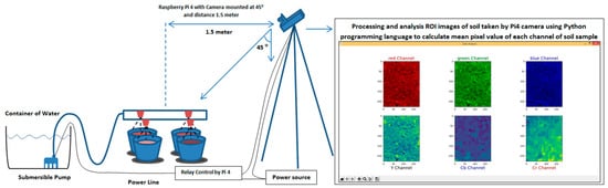
Figure 1. The experimental setup of the proposed imaging system.

The experimental setup of the proposed imaging system depended on the observation and analysis of soil color through processing images taken using an algorithm written in the Python 3.10 programming language. The experiment was undertaken using two samples of soil (sand soil and peat moss soil) under three different scenarios, as shown in Figure 2 and Table 1, where every scenario had over 300 sample images. The first scenario was executed on a dusty day, the second scenario was cloudy, and the last scenario was sunny. All images in this experiment were taken in real-time through an RPi 4 camera for processing to decide whether irrigation was required.

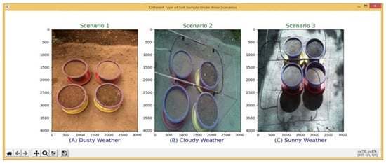
Figure 2. Data collection under three scenarios: (A) dry-dusty; (B) dry-cloudy; (C) dry-sunny.

Table 1. Data collection scenarios.

No. of Soil Types per Scenario	Exp. Scenario	Conditions
1, 2	Dusty	Dry
		Wet
1, 2	Cloudy	Dry
		Wet
1, 2	Sunny	Dry
		Wet

Furthermore, improving the quality and reliability of collected data involved choosing the appropriate sensor type and installing it correctly. Yet, in order to be helpful in making timely and well-informed irrigation decisions, the data needed to be available. Accessing the data gathered by soil moisture sensors can be performed either automatically or manually. To obtain data manually, one must go to the sensor location and utilize the integrated gauges and screens to read the data, or they can connect a reader, laptop computer, or other portable device to download the data. Since there are fewer data transmission units with manual access, it is typically less expensive than automatic access. Wireless signal transmission may be impeded by towering foliage, as shown in Figure 3a. Extending the antenna may be a solution in this case. With shorter vegetation, signals can be transferred more easily, as shown in Figure 3b.

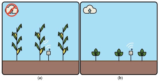
Figure 3. Data transmission with (a) Tall vegetation may block the transfer of the wireless signal, and (b) Extending the antenna may be a solution in this case (with shorter vegetation, signals can be transferred more easily).

Automated data access via websites and mobile applications is available at any time, based on wireless data transfer to servers. Nearly real-time monitoring is made possible by the databases, which are typically updated every five to thirty minutes. Wireless data transfer can occur at the sensor location via a communication tower or at a base station that connects to several nodes where sensors are located. Certain producers of drip and sprinkler irrigation systems additionally provide the option of connecting soil moisture sensors to the irrigation system’s control panel, after which the data, along with other details like system pressure and flow rate, are sent wirelessly to servers.

When selecting a wireless data transfer method, keep in mind that tall, thick canopies may prevent the antennas from transmitting a signal. In certain situations, longer antennas might be required. There may be situations where even the extended antennas are unable to transmit a wireless signal, necessitating the use of additional signal relay capabilities (as well as the related expenditures and equipment).

3.2. System Framework and Hardware Design

This paper proposes an automatic irrigation system that recognizes soil images as wet or dry. The captured soil image passes through three stages before achieving the classification result that includes the following: the preprocessing stage, which includes ROI detection, segmentation, and storage; and the feature extraction stage. The mean value is computed for every channel individually to create a dataset for use in the next stage. Finally, the classification stage uses a random forest algorithm to classify the soil image. The block diagram of the proposed imaging system is shown in Figure 4. The system framework consists of two main parts: the hardware design for capturing images and controlling irrigation processes and the software for analyzing soil image color and undertaking irrigation control.

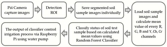
Figure 4. The block diagram of the proposed imaging system.

The automatic selection of the region of interest (ROI) detection and ROI segmentation are shown in Figure 5. In an open loop system, the operator makes the decision on the amount of water to be applied and the timing of the irrigation event. The controller is programmed correspondingly and the water is applied according to the desired schedule. Open loop control systems use either the irrigation duration or a specified applied volume for control purposes. Open-loop controllers normally come with a clock that is used to start irrigation. Termination of the irrigation can be based on a pre-set time or may be based on a specified volume of water passing through a flow meter (Boman et al. 2006).

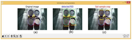
Figure 5. Detection and segmentation of ROI.

3.2.1. Soil Image Dataset

The entire frame size of the captured image is shown in Figure 5. It was designed to preprocess and segment only soil samples, considering all soil types (4 planting pots). These segmented images were stored sequentially to create a dataset including different soil appearances captured at different times. Using the Hough transform technique [24] to detect and segment planting pot by replacing the detected circle with a rectangle border, the center of the detected shape was then taken as a reference point to crop the soil sample by holding a fixed pixel size around 227 × 180 pixels of detection border as shown in Figure 5c.

The next step was loading cropped-stored images, as shown in Figure 6, to calculate the mean values of (R, G, B) and (Y, Cb, and Cr) channels for every single image and saving these values in Excel format sequentially to create the dataset used in the machine learning model. The total number of stored images in the overall collected samples was 900 feature rows and 6 columns. The equations below represent the mean value calculations of all channels.

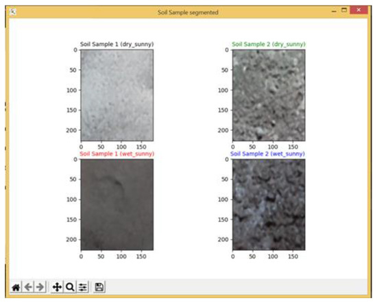
Figure 6. Segmentation of every sample individually to calculate the mean pixel value for RGB channels.

The intensity $i_c$ was obtained by averaging all image pixel values within the selected ROI as follows:

$$i_c=\frac{{\sum }_{x,y\in ROI}I\left(x,y\right)}{\left|{ROI}_1\right|}$$

(1)

where $I\left(x,y\right)$ is the intensity pixel value at the image location ($x,y$) and $\left|{ROI}_1\right|$ is the size of the selected ROI for the soil type. Similarly, for Gm, Bm, Ym, Cbm, and Crm channels, Rm is the red channel. The mean value, k, is the number of image pixels, and rn represents pixel value.

3.2.2. Soil Image Analysis

In an image processing context, every image is composed of intensity and color that combine to form an integrated picture. The image color space [25,26] can be classified according to the types of channels included, such as RGB, HSV, YUV, CMYK, and YCbCr [27] color spaces and so on. This study utilized RGB images captured by the Pi 4 camera, which were converted to YCbCr images to extract three different channels: R (red channel), G (green channel), and B (blue channel). Also, Y-luminance (luma), Cb (blue-difference), and Cr (red-difference) can be used for analyzing soil color easily. The soil color brightness values are affected by different weather conditions, such as dusty, cloudy, and sunny. On the other hand, the surface color of wet soil is also different from the surface color of dry soil. These different situations are considered to help us analyze the soil color to estimate if it needs to be irrigated or not. The brightness effect can be observed in Figure 6 by taking a histogram for the same sample of peat moss-type soil in the cases of wet and dry, giving two different mean values.

After that, the ROI of the soil samples was cropped and saved individually and automatically using an algorithm written in Python 3.10. In the next step, the system read the stored images to calculate the mean value for each channel individually, which ranged from 0 to 255 and was computed using the Stat function from the Image Stat library installed in the virtual Python environment using the PyCharm program.

The threshold value was selected based on the mean value of each channel of the color image through the use of over 300 sample images for each scenario under the (wet, dry) conditions where the total number of image samples became over 900 sample images. This threshold, for every case, is used as a reference value (collected from 900 sample images) to compare the real-time computed results for (R, G, B and Y, Cb, Cr) channels with reference to pre-computed results (R, G, B and Y, Cb, Cr) channels. The threshold values for each scenario are illustrated in Table 2. Finally, the system works fully automatically by taking out the soil image in real time and extracting features that compare with the data set feature to make the irrigation decision.

Table 2. The threshold values under different scenarios.

Soil Type	Exp. Scenario	Condition	Threshold Value for RGB and YCbCr Channels, Respectively
Peat moss soil	Dusty	Dry	(146, 90, 57, 87, 106, 161)
Sandy soil			(213, 140, 92, 134, 98, 172)
Peat moss soil		Wet	(77, 9, 2, 15, 118, 163)
Sandy soil			(45, 39, 6, 30, 110, 136)
Peat moss soil	Cloudy	Dry	(99.58, 96.39, 95.27, 96.43, 127.20, 129.70)
Sandy soil			(133.89, 144.22, 146.62, 143.74, 129.98, 122.50)
Peat moss soil		Wet	(51.98, 56.20, 55.99, 55.68, 128.28, 126.09)
Sandy soil			(84.41, 90.64, 85.24, 88.43, 125.78, 125.86)
Peat moss soil	Sunny	Dry	(126.38, 127.12, 125.08, 126.3, 126.96, 127.99)
Sandy soil			(96.46, 99.26, 102.29, 99.88, 129.82, 126.18)
Peat moss soil		Wet	(84.70, 83.86, 87.57, 85.06, 129.84, 127.79)
Sandy soil			(90.74, 87.47, 86.31, 87.45,126.94, 129.67)

From Table 2, the variation of the mean value of the same soil sample in different scenarios can be observed. For example, the first row of dusty/dry conditions contains RGB and YCbCr mean values, respectively, of peat moss soil samples, which are different in cloudy/dry conditions and sunny/dry conditions. This concept is the same in all other cases caused by variations in the luminance value.

3.2.3. Random Forest Classifier Model

A random forest is a meta-estimator that fits many decision tree classifiers on various sub-samples of the dataset and uses averaging to improve predictive accuracy and control over-fitting. The RF classifier model can be applied in the classification stage to recognize the soil class. The soil training dataset was used as an input feature with their corresponding classes and the testing dataset, where the output is the soil class in the testing soil dataset. The RF is considered a suitable machine learning tool with higher stability by combining multiple de-correlated decision trees, especially when dealing with a large dataset which consists of a cluster of tree estimators based on a bagging technique using a training dataset randomly sampled through all tree branches in the forest, where every tree gives an estimated result which determines the class, as shown in Figure 7. The randomized samples affect the tree’s construction when selecting the node and the coordinate of dividing the tree [28]. The RF algorithm mechanism is as follows:

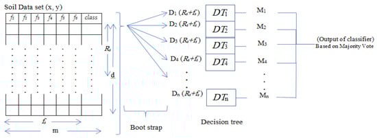
Figure 7. The RF algorithm mechanism.

• Drawing M-tree bootstrap samples from the training data.
• For each of the bootstrap sample data entries, growing an un-pruned classification tree.
• At each internal node, randomly selecting an entry from the N predictors and determining the best split using only those predictors.
• Saving the tree as-is, alongside those built thus far (not performing cost complexity pruning).
• Forecasting new data by aggregating the forecasts of the M-tree trees.

RF is ideally suited for the analysis of complex ecological data. RF predictors are an ensemble-learning approach based on regression or classification trees. Instead of building one classification tree (classifier), the RF algorithm builds multiple classifiers using randomly selected subsets of the observations and random subsets of the predictor variables. The predictions from the ensemble of trees are then averaged in the case of regression trees, or tallied using a voting system for classification trees. RF is efficient to support flexible modelling strategies. RF is capable of detecting and making use of more complex relationships among the variables. RF is unexcelled in accuracy among current algorithms and does not over-fit. It also generates an internal unbiased estimate of the generalization error as the forest building progresses. Potential applications of RF to ecology include the following: classification and regression analysis, survival analysis, variable importance estimate, and data proximities. Proximities can be used for clustering, detecting outliers, multiple dimensional scaling, and unsupervised classification. RF can interpolate missing values and maintain high accuracy even when a large proportion of the data are missing. RF can handle thousands of input variables without variable exclusion. It runs efficiently on large databases. RF can also handle a spectrum of response types, including categorical, numeric, ratings, and survival data. Another advantage of RF is that it requires only two user-defined parameters (the number of trees and the number of randomly selected predictive variables used to split the nodes) to be defined. These two parameters should be optimized in order to improve predictive accuracy. In recent years, RF has been widely used by ecologists to model complex ecological relationships because they are easy to implement and easy to interpret.

3.3. Evaluation Metrics

Confusion matrix, accuracy, precision, recall, F1 score, and MCC are a few of the common assessment measures that were used to assess the RF model’s performance. The confusion matrix, which displays the quantity of true positive (TP), true negative (TN), false positive (FP), and false negative (FN) predictions, offers a tabular depiction of the model’s performance. The ratio of correct forecasts to total forecasts is known as accuracy. The precision, also referred to as a positive predictive value, represents the percentage of TP forecasts among all of the model’s positive predictions. Recall, often called sensitivity or TP rate, is the percentage of true positive cases among all TP forecasts. The balance between accuracy and recovery is captured by the F1 score, which is a harmonic measure of both. It offers a single metric to evaluate the accuracy and recall of the model at the same time. Last, the MCC is a quality metric for binary classification models that takes TP, TN, FP, and FN predictions into account. It assesses the degree of agreement between the true and predicted labels overall, with a score of +1 denoting a perfect prediction, 0 a random prediction, and −1 a total disagreement. The definitions of these variables are as follows:

Accuracy = (((TP + TN)))/(((TP + TN + FP + FN)))

(2)

Precision = TP/(((TP + FP)))

(3)

Recall = TP/(((TP + FN)))

(4)

F1Score = ((2 × (Precision × Recall)))/(((Precision + Recall)))

(5)

MCC = (((TP × TN − FP × FN)))/√(((TP + FN)(TN + FP)(TP + FP)(TN + FN)))

(6)

4. Experimental Results

4.1. Hardware

The Raspberry Pi 4 Model B that was used in this study can be used as a stand-alone mini-computer, having a Quad-core Cortex-A72 processor (ARM v8) 64-bit SoC @1.5GHz and 2GB LPDDR4-3200 SDRAM, wireless, Bluetooth 5.0, BLEGigabit Ethernet, and standard 40 pin GPIO headers. The GPIO 4 pin was used to drive the relay circuit to activate an AC submersible water pump. The Pi 4 microcontroller is suitable for many advanced applications because of its small size, efficient interrupt structure, and ease of programming with open-source Python software (IDE). Also, the Pi can be easily linked to a computer through an Ethernet cable or wirelessly to receive and transmit data. The hardware design for the proposed imaging smart irrigation system is shown in Figure 8.

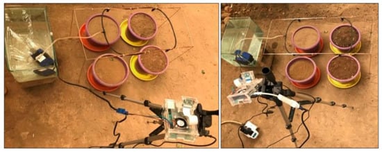
Figure 8. The hardware design of the proposed imaging system.

The classification result was interpreted as a command sent via the GPIO pin of Pi4 to control the relay driving circuit to turn on/off the submersible water pump through the irrigation process. The proposed system’s experimental results were achieved using PyCharm Community Edition 2022.1 supported with library access (OpenCV, NumPy, Image Stat, pandas, sklearn, and matplot libraries) and implemented in the Raspberry Pi4 operating system Debian version: 11 (bullseye). The soil state prediction is based on image gradient familiarity using R, G, B and Y, Cb, Cr information in the RF classifier that provides an accurate correlation between the tested image and its class. The 900 samples of the soil color dataset were split with 90% being randomly sampled into the decision trees for model training and the remaining 10% for testing. The histogram of the wet and dry case of the same soil sample is shown in Figure 9.

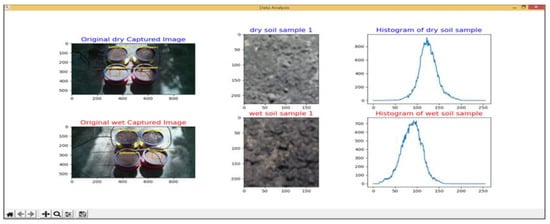
Figure 9. The histogram of the wet and dry case of the same soil sample.

4.2. Evaluation of the RF Classifier Model

The adopted RF classifier parameters were six input layers per sample image utilized with 25 tree estimators. The performance of the RF model was evaluated for classifying soil images into six classes as shown in Table 2. The color intensity data for RGB and YCbCr from each soil’s selected ROI were collected and recorded in an Excel file named “train.csv” to assess the acquired data. First, to assess how well a classification model was performing, a confusion matrix was used to compare the actual results to the predictions made by the RF model, as shown in Figure 10.

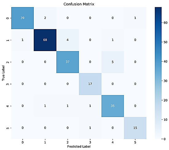
Figure 10. Confusion matrix for testing data.

Figure 10 provides insights into the model’s ability to predict each class correctly for all six cases of both soil types in the different categories of “dusty”, “cloudy”, and “sunny” with a prediction accuracy of 0.921. Furthermore, it is possible to compute a number of performance indicators using the values given from the confusion matrix, including precision, recall, F1 score, and MCC. These indicators offer several viewpoints on how well a categorization model is performing. The precision provides a broad indication of correctness with an accuracy of 0.92 and an F1 score of 0.91, which compromises between precision and recall, whereas the MCC of 0.9 reflected a strong positive correlation, suggesting that RF was a highly effective classification model in this application.

An illustration of the trade-off between recall and precision for a classification model at different thresholds is a Precision-Recall (PR) curve. The PR curve is an evaluation metric that works with unbalanced datasets when one class is significantly more abundant than the other. This is important because even high accuracy may not signify anything if the model can only predict the majority class in imbalanced datasets. On the other hand, PR curves let the viewer comprehend how well the model performs in comparison to the minority class. Figure 11 illustrates the PR curve for different classification thresholds.

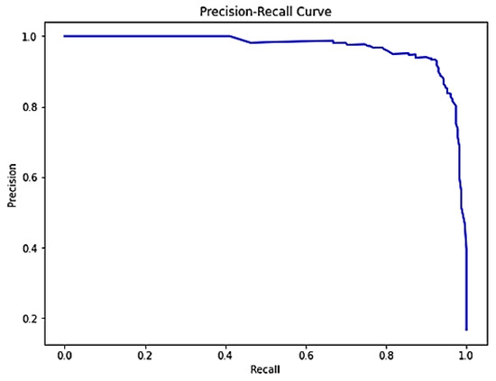
Figure 11. PR Curve on the proposed created dataset.

A Receiver Operating Characteristic (ROC) curve is another curve to illustrate how well the model can distinguish between different classes. When a discriminating threshold is changed, the ROC curve visually depicts the trade-off between the true positive rate (sensitivity) and false positive rate (specificity) for a binary classification system. It is a useful tool to assess how well a classification model performs at different threshold settings. Figure 12 illustrates the ROC curve for different classification thresholds.

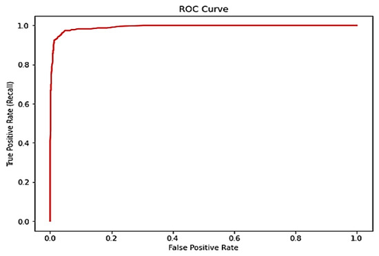
Figure 12. ROC curve on the proposed created dataset.

The histogram of predicted probabilities for all six classes is illustrated in Figure 13, providing insights into the distribution of model confidence scores. Plots of histograms display the distribution of the expected values. The intended outcome is well-defined forecasts that are near 0 or 1, signifying a strong likelihood for any of the two groups. The dataset yielded highly precise estimates, with nearly all probabilities falling between 0 and 1. Even if there is a backdrop of predictions across the range, here the first class generated a larger frequency of probability near 0 or 1 than the other classes.

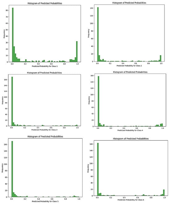
Figure 13. Histogram of predicted probabilities for 6 classes.

The bar chart in Figure 14 represents the importance of each feature in the RF model. Features are sorted in descending order based on their contribution to the model’s decision-making process, where the soil image features such as Cr-channel and Cb-channel are the most dependent in the classification process rather than (R, B, G, and Y) channels via the RF classifier.

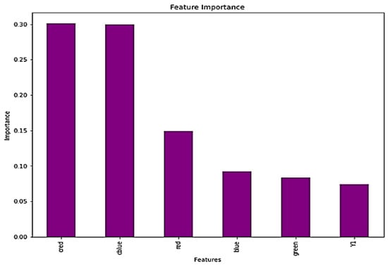
Figure 14. Feature importance.

The box plot in Figure 15 illustrates the distribution of a specific feature between different classes, offering insights into the feature’s discriminatory power.

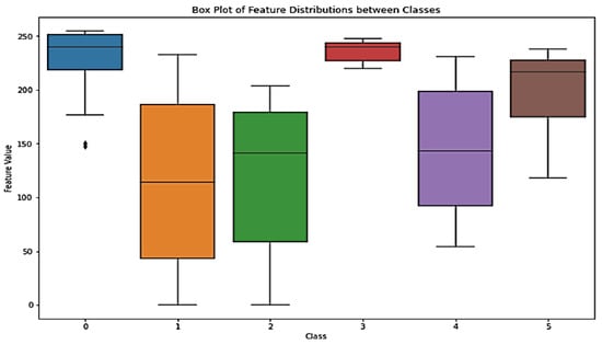
Figure 15. Box plot of feature distribution among classes.

5. Conclusions

This study explored the feasibility of using computer vision technology to evaluate an automatic soil irrigation system by extracting soil sample images in real-time using a Raspberry Pi4 camera in an agricultural environment and classifying these images to identify whether the soil needs to be irrigated or not. In other words, the need for soil irrigation, while taking into consideration the cost, soil type, and weather conditions, is determined by directly analyzing the soil color using a real-time smart imaging system.

The implementation results were satisfactory and achieved the goal of this study, although it presents some limitations, such as the need to implement the experiment on bare ground or locations such as orchards of trees or nurseries of seedlings rather than fields of wheat and barley or similar agricultural applications. Four different soil samples were utilized in this study, two with different types of peat moss soil and others with sandy soil where the color was slightly different, but every type gave a different mean value based on RBG, YCbCr channel analysis. The proposed system can be installed individually in an environment by providing a power source covering the Pi4 requirement and that of the water pump switch, where the Pi4 is responsible for implementing the software and controlling irrigation. Significant power savings are possible by putting the system into sleep mode and only waking it twice a day, which would allow a small solar cell and battery to provide power for the computer and pump control electronics. In future work, the Raspberry Pi should be connected to a network via Wi-Fi to allow remote monitoring and control, and additional soil moisture and humidity sensors could be used to achieve larger training datasets and a lower need for supervision. Hence, for future direction, it is recommended to use the capabilities and availability of cheaper, more sensitive, and sophisticated sensors for gases, particulates, water quality, noise, and other environmental measurements. These types of sensors have improved and are enabling researchers to collect data in unprecedented spatial, temporal, and contextual detail, optimize irrigation algorithms, and/or explore applications beyond traditional agriculture.

References

- Esteva, A.; Chou, K.; Yeung, S.; Naik, N.; Madani, A.; Mottaghi, A.; Liu, Y.; Topol, E.; Dean, J.; Socher, R. Deep learning-enabled medical computer vision. Npj Digit. Med. 2021, 4, 1–9. [Google Scholar] [CrossRef] [PubMed]
- Narendra, V.G.; Hareesha, K.S. Prospects of computer vision automated grading and sorting systems in agricultural and food products for quality evaluation. Int. J. Comput. Appl. 2010, 1, 1–9. [Google Scholar] [CrossRef]
- Tian, H.; Wang, T.; Liu, Y.; Qiao, X.; Li, Y. Computer vision technology in agricultural automation—A review. Inf. Process. Agric. 2020, 7, 1–19. [Google Scholar] [CrossRef]
- Wu, Z.; Chen, Y.; Zhao, B.; Kang, X.; Ding, Y. Review of weed detection methods based on computer vision. Sensors 2021, 21, 3647. [Google Scholar] [CrossRef]
- Azarmdel, H.; Jahanbakhshi, A.; Mohtasebi, S.S.; Muñoz, A.R. Evaluation of image processing technique as an expert system in mulberry fruit grading based on ripeness level using artificial neural networks (ANNs) and support vector machine (SVM). Postharvest Biol. Technol. 2020, 166, 111201. [Google Scholar] [CrossRef]
- Kakani, V.; Nguyen, V.H.; Kumar, B.P.; Kim, H.; Pasupuleti, V.R. A critical review on computer vision and artificial intelligence in food industry. J. Agric. Food Res. 2020, 2, 100033. [Google Scholar] [CrossRef]
- Muhammad, Z.; Hafez, M.A.A.M.; Leh, N.A.M.; Yusoff, Z.M.; Hamid, S.A. Smart agriculture using internet of things with Raspberry Pi. In Proceedings of the 2020 10th IEEE International Conference on Control System, Computing and Engineering (ICCSCE), Penang, Malaysia, 21–22 August 2020; pp. 85–90. [Google Scholar]
- Scheberl, L.; Scharenbroch, B.C.; Werner, L.P.; Prater, J.R.; Fite, K.L. Evaluation of soil pH and soil moisture with different field sensors: Case study urban soil. Urban For. Urban Green. 2019, 38, 267–279. [Google Scholar] [CrossRef]
- Shi, W.; Zhang, S.; Wang, M.; Zheng, W. Design and performance analysis of soil temperature and humidity sensor. IFAC-PapersOnLine 2018, 51, 586–590. [Google Scholar] [CrossRef]
- Al-Naji, A.; Fakhri, A.B.; Gharghan, S.K.; Chahl, J. Soil color analysis based on a RGB camera and an artificial neural network towards smart irrigation: A pilot study. Heliyon 2021, 7, e06078. [Google Scholar] [CrossRef]
- Agrawal, N.; Singhal, S. Smart drip irrigation system using raspberry pi and Arduino. In Proceedings of the International Conference on Computing, Communication & Automation, Greater Noida, India, 15–16 May 2015; pp. 928–932. [Google Scholar]
- Tarange, P.H.; Mevekari, R.G.; Shinde, P.A. Web based automatic irrigation system using wireless sensor network and embedded Linux board. In Proceedings of the 2015 International Conference on Circuits, Power and Computing Technologies [ICCPCT-2015], Nagercoil, India, 19–20 March 2015; pp. 1–5. [Google Scholar]
- Dhanekula, H.; Kumar, K.K. GSM and Web Application based Real-Time Automatic Irrigation System using Raspberry pi 2 and 8051. Indian J. Sci. Technol. 2016, 9, 1–6. [Google Scholar] [CrossRef]
- Ashok, G.; Rajasekar, G. Smart drip irrigation system using Raspberry Pi and Arduino. Int. J. Sci. Eng. Technol. Res. 2016, 5, 9891–9895. [Google Scholar]
- Sharma, S.; Gandhi, T. An automatic irrigation system using self-made soil moisture sensors and Android App. In Proceedings of the Second National Conference on Recent Trends in Instrumentation and Electronics, Gwalior, India, 30 September–1 October 2016. [Google Scholar]
- Chate, B.K.; Rana, J.G. Smart irrigation system using Raspberry Pi. Int. Res. J. Eng. Technol. 2016, 3, 247–249. [Google Scholar]
- Koprda, Š.; Magdin, M.; Vanek, E.; Balog, Z. A Low Cost Irrigation System with Raspberry Pi–Own Design and Statistical Evaluation of Efficiency. Agris-Line Pap. Econ. Inform. 2017, 9, 79–90. [Google Scholar] [CrossRef][Green Version]
- Ishak, S.N.; Malik, N.N.N.A.; Latiff, N.M.A.; Ghazali, N.E.; Baharudin, M.A. Smart home garden irrigation system using Raspberry Pi. In Proceedings of the 2017 IEEE 13th Malaysia International Conference on Communications (MICC), Johor Bahru, Malaysia, 28–30 November 2017; pp. 101–106. [Google Scholar]
- Padyal, A.; Shitole, S.; Tilekar, S.; Raut, P. Automated Water Irrigation System using Arduino Uno and Raspberry Pi with Android Interface. Int. Res. J. Eng. Technol. 2018, 5, 768–770. [Google Scholar]
- Vineela, T.; NagaHarini, J.; Kiranmai, C.; Harshitha, G.; AdiLakshmi, B. IoT based agriculture monitoring and smart irrigation system using raspberry Pi. Int. Res. J. Eng. Technol. 2018, 5, 1417–1420. [Google Scholar]
- Mahadevaswamy, U.B. Automatic IoT based plant monitoring and watering system using Raspberry Pi. Int. J. Eng. Manuf. 2018, 8, 55. [Google Scholar]
- Hasan, M. Real-time and low-cost IoT based farming using raspberry Pi. Indones. J. Electr. Eng. Comput. Sci. 2020, 17, 197–204. [Google Scholar]
- Kuswidiyanto, L.W.; Nugroho, A.P.; Jati, A.W.; Wismoyo, G.W.; Arif, S.S. Automatic water level monitoring system based on computer vision technology for supporting the irrigation modernization. In Proceedings of the IOP Conference Series: Earth and Environmental Science, Yogyakarta, Indonesia, 4–5 November 2020; Volume 686, p. 12055. [Google Scholar]
- Mukhopadhyay, P.; Chaudhuri, B.B. A survey of Hough Transform. Pattern Recognit. 2015, 48, 993–1010. [Google Scholar] [CrossRef]
- Chavolla, E.; Zaldivar, D.; Cuevas, E.; Perez, M.A. Color spaces advantages and disadvantages in image color clustering segmentation. In Advances in Soft Computing and Machine Learning in Image Processing; Springer: Berlin/Heidelberg, Germany, 2018; pp. 3–22. [Google Scholar]
- Sharfina, G.; Gunawan, H.A.; Redjeki, S. The comparison of color space systems analysis on enamel whitening with infusion extracts of strawberry leaves. J. Int. Dent. Med. Res. 2018, 11, 1011–1017. [Google Scholar]
- Tan, Y.; Qin, J.; Xiang, X.; Ma, W.; Pan, W.; Xiong, N.N. A robust watermarking scheme in YCbCr color space based on channel coding. IEEE Access 2019, 7, 25026–25036. [Google Scholar] [CrossRef]
- Belgiu, M.; Drăguţ, L. Random forest in remote sensing: A review of applications and future directions. ISPRS J. Photogramm. Remote Sens. 2016, 114, 24–31. [Google Scholar] [CrossRef]
Disclaimer/Publisher’s Note: The statements, opinions and data contained in all publications are solely those of the individual author(s) and contributor(s) and not of MDPI and/or the editor(s). MDPI and/or the editor(s) disclaim responsibility for any injury to people or property resulting from any ideas, methods, instructions or products referred to in the content. |
© 2024 by the authors. Licensee MDPI, Basel, Switzerland. This article is an open access article distributed under the terms and conditions of the Creative Commons Attribution (CC BY) license (https://creativecommons.org/licenses/by/4.0/).