Abstract
Composite curing through infrared radiation (IR) has become a popular autoclave alternative due to lower energy costs and short curing cycles. As such, understanding and measuring the effect of all parameters involved in the process can aid in selecting the proper constituents as well as curing cycles to produce parts with a high degree of cure and low curing time. In this work, a numerical model that takes inputs such as part geometry, material properties, curing-related properties and applied curing cycle is created. Its outputs include the degree of cure, maximum curing temperature and total curing time. A genetic algorithm and a design of experiments (DOE) sequence cover the range of each input variable and multiple designs are evaluated. Correlations are examined and factor analysis on each output is performed, indicating that the most important inputs are activation energy, specimen precuring, applied curing temperature and curing duration, while all the others can be considered constant. Finally, response surfaces are created in order to effectively map and provide estimations of the design space, resulting in a curing cycle optimizer given certain restrictions over the input parameters.
1. Introduction
Composite materials such as carbon fiber-reinforced polymer composites offer some of the highest strength-to-weight and stiffness-to-weight ratios among all structural materials and can provide major weight reductions and corresponding energy savings (fuel savings during the use of a vehicle, for example) when used to replace traditional structural materials such as steel. However, to fully exploit the fuel savings, an optimized energy-intensive manufacturing process must be employed as the manufacturing of carbon fiber composites, from raw materials to prepreg creation, can require up to 223 MJ/kg until curing [1,2]. The net energy impact depends both on the initial energy expenditure and the fuel savings that accumulate over time during product use. The complex energy tradeoffs and their effect on the net life cycle impacts of composite products have been analyzed in several studies [3,4]. Clearly, composites present a great R&D potential for reducing manufacturing energy intensity (Figure 1).
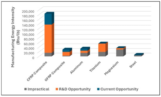
Figure 1.
Comparison of manufacturing energy intensities [3].
While autoclave curing systems are known for producing parts with high quality, their high purchase and running costs, along with long energy-hungry curing cycles, can often be prohibitive (Figure 2) [5,6,7,8,9].
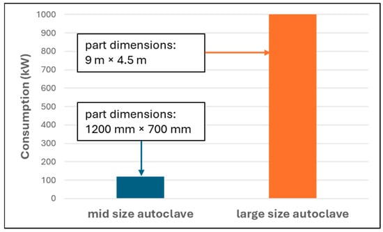
Figure 2.
Comparative consumption of different autoclaves [5,6,7,8,9].
Thus, fast and energy-efficient curing systems are especially interesting to industries, such as automotive, to satisfy the requirements of large-batch production with short cycle duration, compatible with common automatized processes in the sector [10].
While conventional convection and conduction methods are well researched and controllable [11], they exhibit small margins in energy savings [3]. Microwave curing provides an energy-efficient alternative to autoclave curing, showcasing low running and maintenance costs along with potential energy savings of up to 45% [3,11]. However, it requires compatible consumables and particular health and safety measures, and demonstrates low handling flexibility with parts often curing non-uniformly [1,11]. Similarly, radio frequency curing leads to non-uniform curing in irregular shapes with some products lacking a temperature rise in a dielectric field [3,12]. Magnetic induction curing enables high heating rates with low running and maintenance costs [3,11]. However, several issues are reported as limitations of this method. The edge effect and local heating effect as well as requirements for specific coil design for each heating pattern or component geometry prevent the adoption of induction curing on a large scale [3,11,13]. Ultraviolet curing (UV) exhibits low running and maintenance costs but requires UV-curable materials and, due to low penetration capabilities, is limited to mostly thin films and coatings [11,14,15,16]. UV curing on thin composites (≤2 mm) has been applied by Saenz-Dominguez et al. [17] along with numerical modeling for the degree of cure prediction, but requires the use of photoinitiators. Electron beam curing requires high installation costs and trained operators while resulting in subpar cured surfaces [16,18]. It is used mostly in thin films or in conjunction with other curing methods (microwave curing) as shown by other researchers [19]. Among all the alternatives, IR curing seems the most promising curing technique, being able to reach a necessary quality standard while providing an energy cost reduction of 50% [3]. IR is an emerging curing technology for composites due to its high energy efficiency, predictable heating rate (the temperature change in unit time), and volumetric heating mechanism.
The curing of glass fiber-reinforced composites with infrared radiation has been investigated by Kiran Kumar et al. [20]. The authors concluded that it is possible to reduce the curing time by 75% and still reach the same properties as conventional thermal curing. They also found that the distance from the IR source and volume of the composite contributed almost 70% on both the tensile and flexural strength when they analyzed variance. Similar results regarding reductions in curing time were found by Igor Zhilyaev et al. [21], who showed that it is possible to use a 40 °C/min heating rate on their system. However, the mechanical properties were not examined in that study. Alpay et al. [22] studied the developed temperatures during IR heating. The authors showed that for a four-layer structure (3 mm thickness), a maximum difference of 8.94 °C occurred between the top and bottom layer, proving the feasibility of uniform curing.
Regarding numerical modeling of cure kinetics to predict cure, many researchers have provided corresponding works. Okabe et al. [23] paired a curing simulation based on the Arrhenius equation with a molecular dynamics simulation of the cross-linked structure to predict density and Young’s modulus. Struzziero et al. [24] performed autoclave curing simulation on L-shape, flat-panel and T-joint composites in order to minimize the process duration and the maximum temperature overshoot. They connected a genetic algorithm with a finite element solver and created an optimal Pareto Front of the multi-objective problem. Their results indicate reductions up to 50% in process time and temperature overshoot for thick components. Patil et al. [25] performed a coupled thermomechanical analysis, based on the autocatalytic cure kinetics model, to simulate process-induced shape distortions occurring from tool removal after autoclave curing. The error compared to experimental data was up to 20%. Shah et al. [26] performed curing simulations to minimize curing time and residual stresses. A genetic algorithm was used to identify the optimal cure cycle, which, for thick laminates, reduced residual stresses by 47%. Redmann A. et al. [27] performed a kinetic study on a dual-curing epoxy resin used in the DLS printing process. Through DSC, a best-fitting model that involved both autocatalysis and diffusion control was developed to generate different Stage 2 curing cycles. The optimal curing cycle reduced the second-stage curing time by 73% without a significant decrease in the mechanical properties. Yuan et al. [28] used multi-scale modeling to predict the residual stresses of composites during curing. Macroscopic temperature, degree of cure gradients and curing residual stresses are calculated and used by representative volume elements (RVEs) to calculate the micro-scale residual stresses for different composite architectures. Their results indicate that the diamond-array RVE exhibited the highest residual stresses while the square-array RVE showed the lowest residual stresses. Jouyandeha M. et al. [29] studied the nonisothermal cure process of an epoxy nanocomposite containing Mn-doped Fe3O4 nanoparticles. Their results indicate that the autocatalytic is a suitable model to express cure kinetics of the examined materials, while the additives resulted in about 17% lower activation energy values compared to neat epoxy. Moreover, MnxFe3-xO4 nanoparticles increased the average autocatalytic reaction order, reflected in a drop in the frequency factor.
In all the above works, the feasibility of accurate cure prediction and mechanical properties from the applied curing cycle is evident, with some works optimizing the procedure as well. However, to the best of our knowledge, we found no study that captures the effect of each input variable on the total outcome. Also, no complete parametric optimization procedure of the IR curing was found. Hence, in this work, a parametric study of all the factors (part geometry, material properties, curing cycle) affecting the curing of a unidirectional (UD) composite through IR is performed. The goal is to identify the factors with the highest significance while also providing a framework for optimizing the procedure (low curing duration with high degree of cure) for different input variables (part geometry, material properties, etc.). Finally, the use of response surfaces enables the identification and prediction of designs that are not simulated but can be used as optimal solutions.
2. Workflow and Input Variables Properties
A simplified workflow of the current study is presented in Figure 3. Initially, a design of experiments is created involving different combinations of part geometry, material properties and IR heating cycle data. Then, a finite element model is created and used to simulate the IR curing process. A genetic algorithm is employed to optimize the curing process by creating designs with a high degree of uniform curing and permissible heat build-up. The above procedure is performed until all designs have been evaluated. Factor analysis is performed to identify the significant factors affecting the process while the data generated from the analysis are used to train response surfaces capable of producing the optimal cure cycle. In the rest of Section 2, each parameter used as input in the FEM solver will be identified along with its range and step. Range defines the variation between the upper and lower limits of each parameter, while step determines how finely the parameter space is sampled. To limit the computational cost, the average number of steps inside each parameter’s design space is 4–6, while parameters that exhibit large ranges, with high variance, or have been shown by the literature to affect the results in a significant manner can have more than 20 steps. Finally, parameters that depend on the use case (e.g., geometry) and display small parameter ranges have 2–3 steps inside the design space.
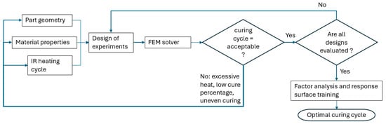
Figure 3.
Problem approach flowchart schematic.
2.1. Geometry
Geometric complexities will be studied in a future analysis after the effect of all other parameters has been examined and validated through experiments. So, in the current study, only flat specimens are considered. As such, the geometry can be parametrically defined by the length of the specimen in the x- and y-directions and its thickness. The maximum in-plane dimension is restricted by the apparatus and should be able to fit inside the area of the emitted radiation from the lamps. The apparatus (Figure 4) that will be used in future analysis can fit specimens of up to 280 mm, so in this study, a range of [100–250] mm is considered. Regarding thickness, most composites in the aeronautic or automotive industries are thin laminates of 1–3 mm. The range and step of each geometric parameter along with the variable name used in the rest of the analysis are given in Table 1.
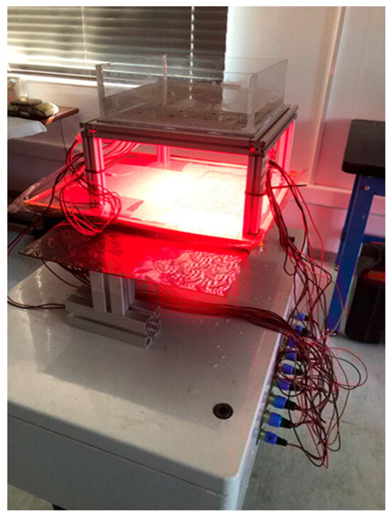
Figure 4.
Example of infrared radiation curing apparatus.

Table 1.
Geometric properties of the numerical model.
2.2. Temperature-Related Material Properties
Table 2 provides all the temperature-related material properties with the corresponding range and step in the design space. The volume fraction for aeronautic and automotive applications ranges from 0.3 to 0.6 as lower values result in low mechanical properties and higher values lead to manufacturing errors [30,31,32,33]. The orthotropic thermal conductivity depends significantly on the direction of the fibers and the fiber volume fraction. Significantly, higher values are observed in the fiber direction, due to the higher thermal conductivity of the reinforcement, while in the other directions, values closer to the resin thermal conductivity are observed [34,35,36]. Unlike thermal conductivity, specific heat capacity is a property dependent on the constitution of the composite, rather than the direction of the reinforcement, with the rule of mixtures providing good estimates [37,38]. Thus, using the properties of the constituents [39,40] with the rule of mixtures (Equation (1)), the effective specific heat capacity can be calculated, with many researchers providing results corresponding to the region indicated in Table 2 [41,42].
where is the composite’s effective specific heat, is the fiber volume fraction, is the specific heat capacity of the reinforcement and is the specific heat capacity of the matrix.
Table 2.
Temperature-related material properties.
Similarly, the density can be calculated from Equation (1) by applying the density of the reinforcement on the term and the density of the matrix on the term , with many researchers providing the range presented in Table 2 [30,33,36,41,43].
2.3. Curing-Related Material Properties
Table 3 provides all the curing-related material properties along with their range and step in the design space. In this study, according to Equation (2), the autocatalytic cure kinetic equation is used, as it is widely used in cure prediction studies [23,25,44,45]:
where is the degree of cure, is the pre-exponential factor, is the activation energy, is the universal gas constant, is the temperature and and are dimensionless constants. The range of each parameter is supported by several studies in the field [43,44,45,46,47,48,49,50].
Table 3.
Curing-related material properties.
2.4. Radiation Data
Table 4 provides all the IR-related material properties and the corresponding range and step in the design space. Absorptivity depends on many factors such as the texture of the surface, material, wavelength and temperature. For our case, an infrared region with rough, dark surfaces, grey incident radiation can be assumed, with absorptivity values in the corresponding region [51,52,53]. The curing temperature and duration span are applied in a big range to cover all possible resin formulations, while the time required to reach the temperature of the curing cycle depends on the heat generation capabilities of the apparatus.
Table 4.
IR-related properties.
2.5. Analytical Workflow and Genetic Algorithm Implementation
The analytical workflow of the current multi-parametric study is depicted in Figure 5. Essentially, geometric data (length in x-direction, length in y-direction, thickness), temperature-related material properties (density, orthotropic thermal conductivity, specific heat, fiber volume fraction), curing-related material properties (pre-exponential factor, activation energy, power m, power n, heat of reaction, initial degree of cure, maximum degree of cure) and radiation data (absorptivity, temperature, time to reach curing temperature, cure duration) are fed into a finite element solver (ANSYS) to simulate the process. Each design’s output involves the average degree of cure of all the elements, the minimum degree of cure on a single element exhibiting the lowest value, the maximum temperature observed during the simulation and total time, which is the sum of the time required to reach the applied temperature, and the curing duration.
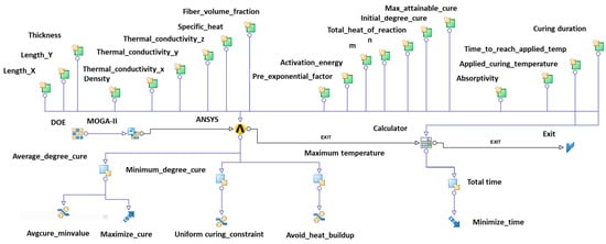
Figure 5.
Analytical workflow.
The Sobol algorithm is a proven exploration DOE generator, so a sequence of 60 Sobol points is chosen to eliminate subjective bias and allow a good initial sampling of the configuration space [54,55,56]. The above exploration DOEs serve as the starting point for the subsequent optimization process, connected to a multi-objective genetic algorithm (MOGA-II). The parameters of the genetic algorithm are presented in Table 5. The 60 initial points along with the 15 generations lead to a total of 900 evaluated designs with a computational cost of 70 h. Increasing the number of Sobol points and number of generations leads to unreasonable computational costs, while 900 designs are deemed satisfactory in the context of this analysis.
Table 5.
MOGA-II settings.
The objectives are to maximize the average degree of cure and minimize total time. The objective function penalizes violations of constraints (Treat constraints). Based on Tournament selection (Probability of selection) MOGA-II chooses solutions for reproduction. Then, it applies cross-over operators (Probability of directional cross-over, Random generator seed) to pairs of parent solutions to generate offspring solutions. Finally, mutation operators (Probability of mutation, Random generator seed) are applied to the offspring solutions. By enabling elitism, the best solution from the current population is carried over to the next generation without any modification. The combined population of parents and offspring is ranked based on Pareto dominance:
where are solution vectors and is the i-th objective function.
Solutions with the same Pareto rank are sorted based on the crowding distance. Crowding distance measures the density of solutions around each solution in the objective space:
where is the crowding distance and and are solutions adjacent to in sorted population.
Solutions for the next generation are selected from the combined population based on Pareto dominance and crowding distance.
Finally, the following constraints are added to achieve a complete, uniform cure without excessive heat built up:
- Average cure constraint (average degree of cure: minimum value ≥ 0.93): high degree of cure.
- minimum cure constraint (minimum degree of cure: minimum value ≥ 0.9): uniform curing.
- Maximum temperature constraint (maximum temperature observed during simulation ≤ 210): avoids excess heat generation and resin carbonization.
The data are split into 80% and 20% samples, used for training and validation, respectively. Since the DOE is not fully factorial and activation energy is the dominant factor in the analysis, the 20% validation points are equally spread across the activation energy range. R-squared is chosen as the metric for validation of the response surface methodology (RSM). The first form of response surfaces is based on the kriging interpolation method with data normalization:
where is the kriging estimate at the unobserved location , is the observed value at location and are the kriging weights.
The kriging weights and the variance of the estimation error can be obtained by solving the kriging system of equations:
where is the covariance between and , and is a Lagrange multiplier used in the minimization of the kriging error to honor the unbiasedness condition.
The Gaussian variogram model is chosen with its formulation being
where is the variogram value at separation distance , is the sill (variance of the process) and is the range (distance at which the correlation between values is negligible).
The covariance function is related to the variogram by
The parameters and are estimated by maximizing the likelihood function. The log-likelihood function for the kriging model is
where is the vector of variogram parameters, is the vector of observed values and is the covariance matrix.
The second form of response surfaces is based on classical feedforward Neural Networks, with Levenberg–Marquardt back propagation chosen as the training algorithm. Network sizing is automatically handled by the software.
The output of the k-th neuron in the output layer is given by
where is the weight from the j-th neuron in the hidden layer to the k-th neuron in the output layer, is the output of the j-th neuron in the hidden layer, is the bias term for the k-th neuron in the output layer and is the activation function used in the output layer.
The output of the j-th neuron in the hidden layer is given by
where is the weight from the i-th neuron in the input layer to the j-th neuron in the hidden layer, is the input to the i-th neuron in the input layer, is the bias term for the j-th neuron in the hidden layer and is the activation function used in the hidden layer.
In this study, rectified linear unit (ReLU) is used as the activation function, while the loss function is mean squared error (MSE):
where is the number of samples or data points, is the actual or observed value for the i-th sample and is the predicted or estimated value for the i-th sample.
Finally, Multivariate Polynomial Interpolation based on the Singular Value Decomposition (SVD) algorithm with a 3rd-degree polynomial function and variable normalization is chosen for the fitting of the 3rd response surface option. The vector of the coefficient can be obtained by solving the system of linear equations using Singular Value Decomposition:
where is the matrix of the input variables and is the vector containing the values of the target variable corresponding to each data point.
The SVD of matrix is given by
where and are orthogonal matrices and is a diagonal matrix containing the singular values. The vector of the coefficient can then be obtained as follows:
The genetic algorithm implementation and the response surface creation are performed in ModeFRONTIER software version 2014 [57].
3. Numerical Modeling
This study aims to capture the curing phenomenon through time, so the parametric geometry is meshed, and transient thermal analysis is performed in ANSYS [58]. Briefly, 20-Node Hexahedral Thermal Solid elements are used with their type being SOLID279. The element has one degree of freedom, namely the temperature, at each node. To accurately capture convection with strong gradients, a consistent convection matrix is applied, by setting the option of KEYOPT(5) to a value of 1 [58].
Figure 6 shows the applied boundary conditions used to simulate the process. The radiation boundary condition is applied at the top surface (Figure 6D) according to Equation (16):
where is the radiation heat transfer rate, is the Stefan–Boltzmann constant, is the surface area of the object, is the emissivity or absorptivity (due to gray body radiation assumption) of the object and is defined as an input parameter in Table 4, is the curing temperature occurring from the IR lamps and specified as input property in Table 4 and is the temperature of the object at each timestep.
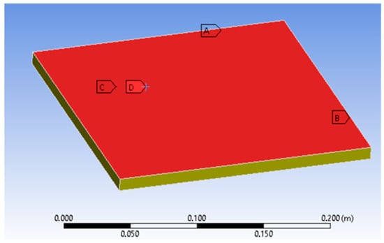
Figure 6.
Applied boundary conditions.
The side surfaces (Figure 6A,B) and bottom surface (Figure 6C) exhibit convection and radiation thermal losses with the environment according to Equations (16) and (17).
where is the convection heat transfer rate, is the convection heat transfer coefficient, is the surface area, is the surface temperature of the object and is the temperature of the surrounding air (22 °C). The convective heat transfer coefficient of air can be estimated utilizing the Nusselt number, in which the Nusselt number itself varies, depending on problem geometry and flow conditions [59]. For this case (natural convection), the studied geometry consists of planar surfaces, so the convection coefficient can be estimated as 5 for the side surfaces and 2 for the bottom surface. These values are provided in ANSYS [58] and are also supported by heat transfer theory [60,61,62].
An iterative solver with a Newton–Raphson method is chosen and the heat convergence criterion is enabled, with the value automatically calculated by the solver () to be acceptable. Regarding the selection of timestep and mesh size, a convergence analysis for the mean case is performed according to Figure 7. The dense grid ensures mesh convergence, while a relatively low timestep size has to be chosen to accurately capture the designs with low heat of reaction, low activation energy and high applied temperature. The above values can capture the transient nature of the phenomenon while also providing reasonable computational cost.
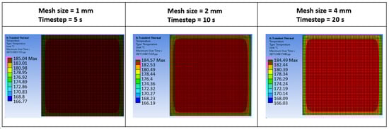
Figure 7.
Maximum temperature results for the mesh and timestep convergence analysis.
4. Results
Before examining the results and obtaining conclusions, the correlation between the inputs of the analysis has to be examined. A partial correlation coefficient is chosen as it provides more accurate results in non-full factorial designs (for 20 input variables with three to five levels each, a full factorial analysis would result in unreasonable computational cost). Since each variable provides a different quantity in the examined problem, the inputs should be uncorrelated. These are presented in Figure 8, where the correlation matrix between inputs exhibits the highest value of 0.272. This serves as an initial validation test of the data presented in this work.
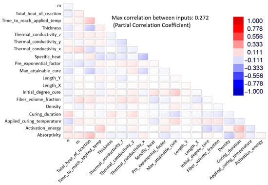
Figure 8.
Correlation matrix of the input variables.
To examine the effect of each parameter on each output (explained in Section 2.5), a factor analysis is performed using the Student method. Figure 9 shows the main factors (high significance) of each output variable. The average and minimum degrees of cure (Figure 9A,B) exhibit the same factors: initial degree of cure, activation energy and applied curing temperature. Precured specimens (~10% degree of cure) tend to slightly cure more uniformly, while, as expected, higher applied temperatures lead to higher overall cure values. Low activation values mean that lower energy requirements are needed to complete the process, and thus, an inverse effect is reasonable. The main factors affecting total curing time (Figure 9C) are cure duration, activation energy and power n. Total curing time is linearly dependent on cure duration, while higher activation energy values indicate that more energy is required to be provided, which, for a constant temperature, translates to higher curing times. Higher power n values indicate an increased rate of reaction at low curing percentages, while a slower rate of reaction at high percentages results in slightly longer total cure times. As expected, the main factor affecting maximum measured temperature (Figure 9D) during the analysis is the applied curing temperature, which further validates the numerical results. Lower activation energy values indicate that the curing reaction is more easily started and the exothermic heat is more rapidly generated, especially at higher applied temperatures. Initially, uncured specimens possess more exothermic heat generation capabilities (higher total heat of reaction), which is contradictory to the findings of higher measured temperatures. However, due to the low range of initial degree of cure [0–0.1] and its effect size (value of 36), being almost at the value of the high-significance criterion (≥30), the result can be regarded as negligible.
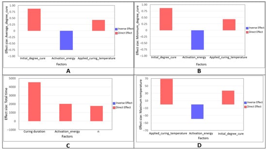
Figure 9.
Factor analysis for output variable: (A) average degree of cure; (B) minimum degree of cure; (C) total cure duration; (D) maximum temperature.
Finally, Figure 10 indicates the Pareto Front of time minimization with respect to applied temperature, where designs with high Pareto dominance (Equation (4)) are highlighted in green. Higher temperatures complete the curing process faster, while applied temperatures over 194 °C produce designs that violate the max temperature constraint.
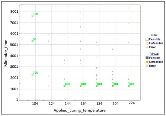
Figure 10.
Pareto Front of time minimization with respect to applied temperature.
Table 6 indicates the predictive performance of each response surface type on each output. The Neural Network outperforms kriging and SVD in terms of curing prediction, while kriging exhibits the highest score in the maximum temperature prediction. All models exhibit high accuracy in total curing time due to their simple forms. Figure 11 plots the predictions of the kriging response surface methodology. Average degree of cure (z-axis) is plotted with activation energy (x-axis) and applied curing temperature (y-axis), with all the other variables at mean value (Table 1, Table 2 and Table 3). The model has captured the non-linearity exhibited in the problem while also indicating that higher activation energy values require higher temperatures to achieve a high degree of cure. The above, along with the absence of unreasonable points and local extrema, further validates the results.
Table 6.
Predictive performance of each RSM.
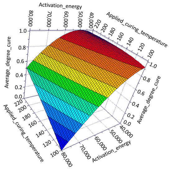
Figure 11.
Prediction of average degree of cure with respect to activation energy and curing temperature using the kriging response surface methodology.
In Figure 12, through the use of the RSM, factors that displayed minimal effect on curing results during the factor analysis are examined. In Figure 12A,B, density, specific heat, power m, and thermal conductivity in the x-direction are set at the lower and upper ends (Table 2 and Table 3), respectively. All other input parameters are set at mean values. The occurring RSM plots present high similarity between them and with the RSM plot, with all parameters at mean values (Figure 11). This validates that these parameters contribute negligibly to the curing results.
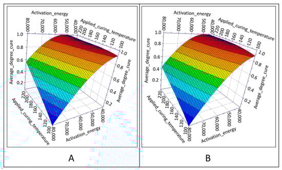
Figure 12.
Comparative RSM plots with density, specific heat, power m, and thermal conductivity in x-direction at lower end (A) and higher end (B) with all other parameters at mean value.
Figure 13 examines the effect of thickness on both curing and maximum temperature difference throughout the plate. Specifically, the thinnest allowable plate in the design space of this study is compared with the corresponding thickest one, while all other parameters are set at mean values (Table 1, Table 2, Table 3 and Table 4). The degree of cure reveals similar patterns for the thin and thick plates, while differences of 3.5 °C and 8 °C are observed.
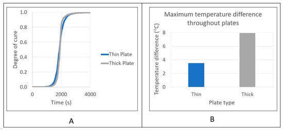
Figure 13.
(A) Comparative degree of cure evolution between thin and thick plates; (B) Comparative maximum temperature difference throughout the thick and thin plates.
Use Case
Finally, to demonstrate and prove the utility of the data-driven models presented in this study, an optimization of the cure cycle of a 2 mm thick plate carbon fiber–epoxy composite is performed. Resoltech® 1070 is chosen as the resin, which possesses a density of 1100 [63]. The cure-related properties were examined by Lascano D. et al. and are given in Table 7 [49]. Their analysis showed very good agreement between experimental and numerical data (autocatalytic model). To capture the average composite case, all temperature-related properties (Table 2) are set at mean values. This choice is further validated since temperature-related properties exhibit low significance in the factor analysis and the density and cure-related properties of the resin are close to the mean values of each parameter presented in this study.
Table 7.
Cure-related properties of Resoltech® 1070 resin [49].
These values are used in the RSM (kriging) to find the cure cycle that enables uniform, complete curing without excessive heat generation within the time constraint of 1 h:
- Average degree if cure ≥ 0.95.
- Minimum degree of cure ≥ 0.95.
- Maximum temperature ≤ 200.
- Total cure duration ≤ 1 h.
Kriging was selected due to its higher accuracy in maximum temperature prediction. The optimal cure cycles are near the maximum temperature constraint, and using NN can result in temperature overshoot and enter the degradation temperature region of the resin. The cure cycles proposed by the RSM are simulated in ANSYS according to Section 3 to account for possible inaccuracies arising from data-driven models, given their overall high but not perfect R-squared values. Also, this way, an assessment between cycles can be performed and the optimal cure cycle can be identified. The corresponding results are given in Figure 14. Essentially, temperatures above 160 °C finish the process (degree of cure ≥ 0.995) between 50 min and 1 h, while temperatures below 120 °C do not provide enough energy to complete the curing of the composite within the time limit. The maximum temperature is 198 °C when applied temperature is 188 °C. In Figure 15, the duration of the cycle produced by the current methodology is compared with the cure cycles proposed by the manufacturer [63] and the cure cycle used by Lascano Diego et al. [49] in specimens used for dynamic mechanical thermal analysis (DMTA). Cure cycle duration reductions of 94% and 44%, respectively, are achieved.
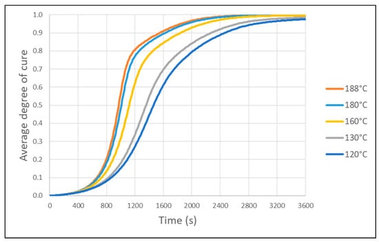
Figure 14.
Cure cycles proposed by the RSM for the use case.
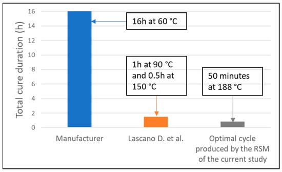
Figure 15.
Comparison of cure cycle duration for Resoltech® 1070 (Lascano D. et al. [49], manufacturer [63]).
5. Conclusions
In this numerical study, the effect of each parameter involved in the IR curing of composites is examined. The range of all parameters involved in the process (geometry, material properties, IR-curing heat transfer) is initially recorded. These data are fed into a finite element solver to obtain the average and minimum degrees of cure, the maximum temperature during curing and curing duration. Through parametric simulation based on 60 Sobol points and a multi-objective genetic algorithm, the effect of each parameter is examined. The results indicate the following:
- All input variables were found to be uncorrelated.
- The curing cycle was mostly dependent on resin properties (activation energy was found to be the most important parameter).
- Higher energy activation values require higher applied temperatures to complete uniform curing but also lead to higher curing duration times.
- Precured specimens (~10% degree of cure) tend to cure slightly more uniformly but have little to no effect on total curing time.
- Thicknesses of [1–3] mm have little effect on the curing results. The max temperature difference throughout the thickest plate (3 mm) is 8 °C and 3.5 °C throughout the slimmest plate for all other parameters at mean value. Similar differences were experimentally observed by other researchers [21].
- Density, specific heat, power m, and thermal conductivity in the x-direction show insignificant effects on the results and can be considered as constants in future analyses.
- Response surfaces are created with the Neural Network outperforming kriging and polynomial SVD in terms of cure prediction but exhibiting smaller accuracy in maximum temperature prediction. All models show excellent accuracy in total cure time prediction.
- Applying the data-driven models on a 2 mm thick composite plate manufactured using Resoltech® 1070 resin resulted in 94% and 44% faster curing compared to the proposed curing duration of the manufacturer [58] and other researchers [44].
Finally, the results presented in this work provide support for a carbon–epoxy or graphene–epoxy (UD) composite, as they are the ones applied typically in aeronautic or automotive applications, where fast and energy-efficient curing systems (IR curing) are required.
6. Future Work
This study deals with the IR curing of composites in automotive or aeronautic applications. In future, more complex cure kinetic models will be examined for resin formulations that deviate from activation-controlled reactions (epoxy–amines). Also, thick laminates (10–15 mm) with different layup orientations will be examined. The process should also be examined from a mechanical point of view, so in the future, the authors will connect the cure kinetics solver with the mechanical one to calculate process-induced distortions, while the numerical results (mechanical properties, degree of cure, energy consumption) will be compared with specimens manufactured from a mid-size autoclave.
Author Contributions
Conceptualization, A.K. and V.K.; methodology, P.G.; software, P.G.; validation, P.G., A.K. and I.K.; formal analysis, P.G.; investigation, P.G.; resources, V.K.; data curation: P.G.; writing—original draft preparation, P.G.; writing—review and editing, A.K. and I.K.; visualization, P.G.; supervision, A.K., I.K. and V.K.; project administration, A.K., I.K. and V.K.; funding acquisition, A.K. and V.K. All authors have read and agreed to the published version of the manuscript.
Funding
This research has received funding from the European Union’s Horizon Europe “REPOXYBLE” under grant agreement 101091891.
Data Availability Statement
The data presented in this study are available on request from the corresponding author. This is because the raw/processed data required to reproduce these findings cannot be shared at this time due to technical/confidentiality restrictions.
Conflicts of Interest
The authors declare no conflict of interest.
References
- Collinson, M.; Bower, M.; Swait, T.J.; Atkins, C.; Hayes, S.; Nuhiji, B. Novel composite curing methods for sustainable manufacture: A review. Compos. Part C Open Access 2022, 9, 100293. [Google Scholar] [CrossRef]
- Song, Y.S.; Youn, J.R.; Gutowski, T.G. Life cycle energy analysis of fiber-reinforced composites. Compos. Part A Appl. Sci. Manuf. 2009, 40, 1257–1265. [Google Scholar] [CrossRef]
- Liddell, H.; Brueske, S.; Carpenter, A.; Cresko, J. Manufacturing Energy Intensity and Opportunity Analysis for Fiber-Reinforced Polymer Composites and Other Lightweight Materials. In Proceedings of the Manufacturing Energy Intensity and Opportunity Analysis for Fiber-Reinforced Polymer Composites and Other Lightweight Materials, Williamsburg, VA, USA, 19–22 September 2016. [Google Scholar]
- Das, S.; Graziano, D.; Upadhyayula, V.K.; Masanet, E.; Riddle, M.; Cresko, J. Vehicle lightweighting energy use impacts in U.S. light-duty vehicle fleet. Sustain. Mater. Technol. 2016, 8, 5–13. [Google Scholar] [CrossRef]
- Manral, A.; Ahmad, F.; Sharma, B. Advances in Curing Methods of Reinforced Polymer Composites. In Reinforced Polymer Composites: Processing, Characterization and Post Life Cycle Assessment; Wiley-VCH Verlag GmbH & Co. KGaA: Weinheim Germany, 2019. [Google Scholar] [CrossRef]
- Available online: https://www.mk-technology.com/?pageID=131 (accessed on 1 March 2024).
- Available online: https://www.alibaba.com/product-detail/PLC-Control-Prepreg-Composite-Carbon-Fiber_1600562371699.html?spm=a2700.7735675.0.0.6dfcAum5Aum5By&s=p (accessed on 1 March 2024).
- Chowdhury, I.R.; Summerscales, J. Cool-Clave—An Energy Efficient Autoclave. J. Compos. Sci. 2023, 7, 82. [Google Scholar] [CrossRef]
- Zaychenko, I.V.; Bazheryanu, V.V.; Gordin, S.A. Improving the Energy Efficiency of Autoclave Equipment by Optimizing the Technology of Manufacturing Parts from Polymer Composite Materials. IOP Conf. Ser. Mater. Sci. Eng. 2020, 753, 032069. [Google Scholar] [CrossRef]
- Available online: https://www.compositesworld.com/articles/fast-and-faster-rapid-cure-epoxies-drive-down-cycle-times (accessed on 1 March 2024).
- Abliz, D.; Duan, Y.; Steuernagel, L.; Xie, L.; Li, D.; Ziegmann, G. Curing Methods for Advanced Polymer Composites—A Review. Polym. Polym. Compos. 2013, 21, 341–348. [Google Scholar] [CrossRef]
- Thermo Energy Corporation. EPRl Radio-Frequency Dielectric Heating in Industry; EPRI: Palo Alto, CA, USA, 1987. [Google Scholar]
- Lucia, O.; Maussion, P.; Dede, E.J.; Burdio, J.M. Induction Heating Technology and Its Applications: Past Developments, Current Technology, and Future Challenges. IEEE Trans. Ind. Electron. 2013, 61, 2509–2520. [Google Scholar] [CrossRef]
- Available online: https://www.zicaichemical.com/news/advantages-and-disadvantages-of-uv-adhesive/ (accessed on 1 March 2024).
- CMendes-Felipe; Oliveira, J.; Etxebarria, I.; Vilas-Vilela, J.L.; Lanceros-Mendez, S. State-of-the-Art and Future Challenges of UV Curable Polymer-Based Smart Materials for Printing Technologies. Adv. Mater. Technol. 2019, 4, 1800618. [Google Scholar] [CrossRef]
- Wali, A.S.; Kumar, S.; Khan, D. A review on recent development and application of radiation curing. Mater. Today Proc. 2023, 82, 68–74. [Google Scholar] [CrossRef]
- Saenz-Dominguez, I.; Tena, I.; Sarrionandia, M.; Torre, J.; Aurrekoetxea, J. An analytical model of through-thickness photopolymerisation of composites: Ultraviolet light transmission and curing kinetics. Compos. Part B Eng. 2020, 191, 107963. [Google Scholar] [CrossRef]
- Gao, C.; Qiu, J.; Wang, S. In-situ curing of 3D printed freestanding thermosets. J. Adv. Manuf. Process. 2022, 4, e10114. [Google Scholar] [CrossRef]
- Zhang, J.; Duan, Y.; Wang, B.; Zhang, X. Interfacial enhancement for carbon fibre reinforced electron beam cured polymer composite by microwave irradiation. Polymer 2020, 192, 122327. [Google Scholar] [CrossRef]
- Kumar, P.K.; Raghavendra, N.V.; Sridhara, B.K. Optimization of infrared radiation cure process parameters for glass fiber reinforced polymer composites. Mater. Des. 2021, 32, 1129–1137. [Google Scholar] [CrossRef]
- Zhilyaev, I.; Brauner, C.; Queloz, S.; Jordi, H.; Lüscher, R.; Conti, S.; Conway, R. Controlled curing of thermoset composite components using infrared radiation and mathematical modelling. Compos. Struct. 2021, 259, 113224. [Google Scholar] [CrossRef]
- Alpay, Y.; Uygur, I.; Kilincel, M. On the optimum process parameters of infrared curing of carbon fiber-reinforced plastics. Polym. Polym. Compos. 2020, 28, 433–439. [Google Scholar] [CrossRef]
- Okabe, T.; Oya, Y.; Tanabe, K.; Kikugawa, G.; Yoshioka, K. Molecular dynamics simulation of crosslinked epoxy resins: Curing and mechanical properties. Eur. Polym. J. 2016, 80, 78–88. [Google Scholar] [CrossRef]
- Struzziero, G.; Skordos, A.A. Multi-objective optimisation of the cure of thick components. Compos. Part A Appl. Sci. Manuf. 2017, 97, 126–136. [Google Scholar] [CrossRef]
- Patil, A.S.; Moheimani, R.; Dalir, H. Thermomechanical analysis of composite plates curing process using ANSYS composite cure simulation. Therm. Sci. Eng. Prog. 2019, 14, 100419. [Google Scholar] [CrossRef]
- Shah, P.; Halls, V.; Zheng, J.; Batra, R. Optimal cure cycle parameters for minimizing residual stresses in fiber-reinforced polymer composite laminates. J. Compos. Mater. 2018, 52, 773–792. [Google Scholar] [CrossRef]
- Redmann, A.; Oehlmann, P.; Scheffler, T.; Kagermeier, L.; Osswald, T.A. Thermal curing kinetics optimization of epoxy resin in Digital Light Synthesis. Addit. Manuf. 2020, 32, 101018. [Google Scholar] [CrossRef]
- Yuan, Z.; Wang, Y.; Yang, G.; Tang, A.; Yang, Z.; Li, S.; Li, Y.; Song, D. Evolution of curing residual stresses in composite using multi-scale method. Compos. Part B Eng. 2018, 155, 49–61. [Google Scholar] [CrossRef]
- Jouyandeh, M.; Paran, S.M.R.; Khadem, S.S.M.; Ganjali, M.R.; Akbari, V.; Vahabi, H.; Saeb, M.R. Nonisothermal cure kinetics of epoxy/MnxFe3-xO4 nanocomposites. Prog. Org. Coat. 2020, 140, 105505. [Google Scholar] [CrossRef]
- Mark, T.; Tory, S.; Bruno, B. Simplifying certification of discontinuous composite material forms for primary aircraft structures. In Proceedings of the SAMPE 2010 Spring Symposium & Exhibition, Conference Proceedings, Seattle, WA, USA, 17–20 May 2010. [Google Scholar]
- Abbott, R. Analysis and Design of Composite and Metallic Flight Vehicle Structure; Abbott Aerospace SEZC Ltd.: Collingwood, ON, Canada, 2017. [Google Scholar]
- Khan, J.B.; Smith, A.C.; Tuohy, P.M.; Gresil, M.; Soutis, C.; Lambourne, A. Experimental electrical characterisation of carbon fibre composites for use in future aircraft applications. IET Sci. Meas. Technol. 2019, 13, 1131–1138. [Google Scholar] [CrossRef]
- Parveez, B.; Kittur, M.I.; Badruddin, I.A.; Kamangar, S.; Hussien, M.; Umarfarooq, M.A. Scientific Advancements in Composite Materials for Aircraft Applications: A Review. Polymers 2022, 14, 5007. [Google Scholar] [CrossRef]
- Burger, N.; Laachachi, A.; Ferriol, M.; Lutz, M.; Toniazzo, V.; Ruch, D. Review of thermal conductivity in composites: Mechanisms, parameters and theory. Prog. Polym. Sci. 2016, 61, 1–28. [Google Scholar] [CrossRef]
- Wang, Y.; Tang, B.; Gao, Y.; Wu, X.; Chen, J.; Shan, L.; Sun, K.; Zhao, Y.; Yang, K.; Yu, J.; et al. Epoxy Composites with High Thermal Conductivity by Constructing Three-Dimensional Carbon Fiber/Carbon/Nickel Networks Using an Electroplating Method. ACS Omega 2021, 6, 19238–19251. [Google Scholar] [CrossRef]
- Kim, H.S.; Bae, H.S.; Yu, J.; Kim, S.Y. Thermal conductivity of polymer composites with the geometrical characteristics of graphene nanoplatelets. Sci. Rep. 2016, 6, 26825. [Google Scholar] [CrossRef] [PubMed]
- Lattimer, B.Y.; Goodrich, T.W.; Chodak, J.; Cain, C. Properties of composite materials for modeling high temperature response. In Proceedings of the ICCM International Conferences on Composite Materials, Edinburgh, UK, 27–31 July 2009. [Google Scholar]
- Available online: https://compositeskn.org/KPC/A214 (accessed on 1 March 2024).
- Available online: https://www.engineeringtoolbox.com/specific-heat-polymers-d_1862.html (accessed on 1 March 2024).
- Available online: https://www.engineeringtoolbox.com/specific-heat-solids-d_154.html (accessed on 1 March 2024).
- Ronald, J. Thermal properties of carbon fiber/epoxy composites with different fabric weaves. In Proceedings of the SAMPE International Symposium Proceedings, Paris, France, 26–27 March 2012. [Google Scholar]
- Tranchard, D.P. High Temperature-Dependent Thermal Properties of a Carbon-Fiber Epoxy Composite. 2018. Available online: https://api.semanticscholar.org/CorpusID:150378149 (accessed on 30 January 2024).
- Tranchard, P.; Samyn, F.; Duquesne, S.; Estèbe, B.; Bourbigot, S. Modelling Behaviour of a Carbon Epoxy Composite Exposed to Fire: Part I-Characterisation of Thermophysical Properties. Materials 2017, 10, 494. [Google Scholar] [CrossRef] [PubMed]
- Cruz-Cruz, I.; Ramírez-Herrera, C.A.; Martínez-Romero, O.; Castillo-Márquez, S.A.; Jiménez-Cedeño, I.H.; Olvera-Trejo, D.; Elías-Zúñiga, A. Influence of Epoxy Resin Curing Kinetics on the Mechanical Properties of Carbon Fiber Composites. Polymers 2022, 14, 1100. [Google Scholar] [CrossRef]
- Chen, K.; Zhu, X.; Zhao, G.; Chen, J.; Guo, S. Cure Kinetics of a Carbon Fiber/Epoxy Prepreg by Dynamic Differential Scanning Calorimetry. Int. J. Polym. Sci. 2023, 2023, 5244722. [Google Scholar] [CrossRef]
- Mphahlele, K.; Ray, S.S.; Kolesnikov, A. Cure kinetics, morphology development, and rheology of a high-performance carbon-fiber-reinforced epoxy composite. Compos. Part B Eng. 2019, 176, 107300. [Google Scholar] [CrossRef]
- Abenojar, J.; Del Real, J.C.; Ballesteros, Y.; Martinez, M.A. Kinetics of curing process in carbon/epoxy nano-composites. IOP Conf. Ser. Mater. Sci. Eng. 2018, 369, 012011. [Google Scholar] [CrossRef]
- Liang, J.; Liu, L.; Qin, Z.; Zhao, X.; Li, Z.; Emmanuel, U.; Feng, J. Experimental Study of Curing Temperature Effect on Mechanical Performance of Carbon Fiber Composites with Application to Filament Winding Pressure Vessel Design. Polymers 2023, 15, 982. [Google Scholar] [CrossRef]
- Lascano, D.; Quiles-Carrillo, L.; Balart, R.; Boronat, T.; Montanes, N. Kinetic Analysis of the Curing of a Partially Biobased Epoxy Resin Using Dynamic Differential Scanning Calorimetry. Polymers 2019, 11, 391. [Google Scholar] [CrossRef] [PubMed]
- Karami, M.H.; Kalaee, M.R.; Mazinani, S.; Shakiba, M.; Shafiei Navid, S.; Abdouss, M.; Beig Mohammadi, A.; Zhao, W.; Koosha, M.; Song, Z.; et al. Curing Kinetics Modeling of Epoxy Modified by Fully Vulcanized Elastomer Nanoparticles Using Rheometry Method. Molecules 2022, 27, 2870. [Google Scholar] [CrossRef]
- Available online: https://www.engineeringtoolbox.com/emissivity-coefficients-d_447.html (accessed on 1 March 2024).
- Available online: https://www.engineeringtoolbox.com/solar-radiation-absorbed-materials-d_1568.html (accessed on 1 March 2024).
- Gao, Y.; Gao, L.; Ma, C.; Ma, Z.; Zhang, X.; Peng, G.; Tian, Z. Thermal response of carbon fiber reinforced epoxy composites irradiated by thermal radiation. Mater. Res. Express 2020, 7, 045302. [Google Scholar] [CrossRef]
- Navid, A.; Khalilarya, S.; Abbasi, M. Diesel engine optimization with multi-objective performance characteristics by non-evolutionary Nelder-Mead algorithm: Sobol sequence and Latin hypercube sampling methods comparison in DoE process. Fuel 2018, 228, 349–367. [Google Scholar] [CrossRef]
- Dimov, I.; Georgieva, R. Monte Carlo algorithms for evaluating Sobol’ sensitivity indices. Math. Comput. Simul. 2010, 81, 506–514. [Google Scholar] [CrossRef]
- Available online: https://support.zemax.com/hc/en-us/articles/1500005487181-Understanding-Sobol-sampling (accessed on 1 March 2024).
- Available online: https://www.esteco.com/ (accessed on 1 March 2024).
- ANSYS Thermal Theory Guide; ANSYS, Inc.: Canonsburg, PA, USA, 2019.
- Malekan, M.; Khosravi, A.; El Haj Assad, M. Chapter 6—Parabolic trough solar collectors. In Rosen, Design and Performance Optimization of Renewable Energy Systems; El Haj Assad, M., Marc, A., Eds.; Academic Press: Cambridge, MA, USA, 2021; pp. 85–100. [Google Scholar] [CrossRef]
- Bergman, T.L.; Frank, P. Incropera. Fundamentals of Heat and Mass Transfer, 7th ed.; Wiley: Hoboken, NJ, USA, 2011. [Google Scholar]
- Available online: https://www.engineersedge.com/heat_transfer/convective_heat_transfer_coefficients__13378.htm (accessed on 1 March 2024).
- Available online: https://www.sfu.ca/~mbahrami/ENSC%20388/Notes/Natural%20Convection.pdf (accessed on 1 March 2024).
- Available online: https://www.resoltech.com/en/markets/marine-construction/1070-s-clear-detail.html (accessed on 1 March 2024).
Disclaimer/Publisher’s Note: The statements, opinions and data contained in all publications are solely those of the individual author(s) and contributor(s) and not of MDPI and/or the editor(s). MDPI and/or the editor(s) disclaim responsibility for any injury to people or property resulting from any ideas, methods, instructions or products referred to in the content. |
© 2024 by the authors. Licensee MDPI, Basel, Switzerland. This article is an open access article distributed under the terms and conditions of the Creative Commons Attribution (CC BY) license (https://creativecommons.org/licenses/by/4.0/).