Field Monitoring of Harvest Timing in Brassica rapa subsp. sylvestris Using Portable VIS–NIR Hyperspectral Imaging

Abstract

Advanced sensing technologies increasingly support monitoring and decision-making processes in modern agriculture. This study investigates the feasibility of developing a harvest timing monitoring workflow based on a portable hyperspectral imaging (HSI) system in the visible–near-infrared (VIS-NIR: 400–1000 nm) range, coupled with machine learning. A hierarchical Partial Least Squares–Discriminant Analysis (Hi-PLS-DA) model was developed and tested to discriminate harvestable from non-harvestable plants of Brassica rapa subsp. sylvestris through the identification of open flowers within otherwise closed flower buds in the raceme. The classification included four target plant classes, i.e., green inflorescences, green leaves, yellow flowers, and yellow leaves, along with two non-target classes, background and not-classified (NC), which were included to support the classification process. The predicted hyperspectral images demonstrated a clear distinction between closed and open flowers, supported by satisfactory classification performance (sensitivity, specificity, precision, and F1-score: 0.78–1.00). This workflow proved effective in handling intrinsic outdoor hyperspectral variability, mitigating illumination and canopy texture, and offers useful methodological insights for the possible future integration of HSI-based approaches into automated field applications, paving the way for rapid, real-time harvest decision support.

1. Introduction

The accurate determination of harvest timing is crucial for crop quality and marketability, as the visual appearance and biochemical traits of vegetables change sharply across developmental stages [1]. Growers often base harvest decisions on visual assessment and field experience, guided by morphological cues such as the presence of closed flower buds, head compactness, and leaf color. However, these empirical indicators are often imprecise and subject to observer bias [2]. Moreover, ongoing climate change alters phenological dynamics via shifts in temperature and precipitation patterns; these traditional visual cues may no longer reliably correspond to ideal harvest windows [3]. In this context, digital and precision agriculture technologies are increasingly explored to support data-driven crop management, with successful adoption depending on usability and integration into practical decision-support workflows [4,5].

RGB imaging has become a widely adopted and cost-effective approach for crop phenotyping and flowering detection. For example, Kior et al. [6] highlighted its versatility as a remote sensing tool for plant trait assessment; Song et al. [7] demonstrated that consumer-grade RGB-D cameras can dynamically capture three-dimensional crop structures, supporting phenological analyses without specialized multispectral equipment. However, RGB approaches face intrinsic limits when different plant parts exhibit similar colors, while changes in illumination and sensor sensitivity further limit separability [8,9].

Visible-near-infrared (VIS-NIR) spectroscopy provides a powerful alternative for detecting flowering stages in horticultural crops. By sensing pigments such as chlorophyll and carotenoids, which exhibit specific absorption features in the blue–red and red-edge/NIR regions, VIS-NIR enables reliable discrimination of leaves, stems, and inflorescences even when visual colors overlap [10,11,12]. Spectral vegetation indices have also been effectively applied to detect foliar diseases, such as rust infection in wheat [13]. However, accurate measurements in field conditions generally require close-range or contact acquisition to minimize variability due to illumination and measurement geometry [14].

In this context, hyperspectral imaging (HSI) in the VIS-NIR range has emerged as a powerful tool for crop and food analysis. By capturing contiguous spectral bands while retaining spatial details, HSI provides detailed information on plant phenotypic traits, such as pigment composition (e.g., chlorophyll and carotenoids), leaf biochemical status, and stress indicators [15]. Several recent reviews have demonstrated the effectiveness of HSI for non-destructive quality assessment of root and tuber crops, as well as for both external and internal attributes in fruits and vegetables [16,17,18,19,20]. White-reference calibration is an additional advantage, as it corrects for variations in illumination and sensor response, ensuring reproducible reflectance data under varying environmental conditions [21]. Despite these benefits, field applications of HSI face challenges due to spectral variability introduced by edge effects, micro-shadowing, and sensor noise, which can cause spectral signatures of different tissues to overlap. Under these conditions, the careful design of a representative calibration dataset that adequately covers the intrinsic spectral variability of the scene becomes more critical than simply increasing the number of samples [22]. Thus, specific preprocessing protocols and chemometric strategies are needed to resolve subtle spectral differences and reduce noise impact, enabling the extraction of physically meaningful spectral features that can be directly linked to the physicochemical properties of the analyzed material, as discussed in the context of hyperspectral imaging and chemometrics [23]. The strong collinearity and high dimensionality of HSI data also require robust multivariate and machine-learning methods to extract relevant features and develop reliable predictive or classification models [23,24,25,26].

In recent years, research in precision agriculture has increasingly emphasized the development of cost-effective, portable, and potentially real-time hyperspectral sensing platforms, together with efficient data processing strategies suitable for field deployment. However, the transition from controlled or laboratory-based hyperspectral systems to portable, field-deployable configurations introduces additional challenges related to environmental variability, canopy complexity, and operational constraints, which still require dedicated investigation and validation through real-field applications [27]. Building on this potential, the present study applies HSI to a case study on the leafy vegetable Brassica rapa subsp. sylvestris, traditionally consumed in Italy as local varieties of “cime di rapa” or “friarielli”, and internationally known as “broccoli rabe”. The quality of this crop is highly dependent on precise harvest timing, as racemes (syn. inflorescences) reach their maximum nutritional, organoleptic, and aesthetic value when they are still green, compact, and closed [28]. In contrast, flower opening (anthesis), evident from the appearance of yellow petals, together with any leaf chlorotic events, adversely affects consumer visual perception, key nutrients, and, ultimately, marketability [29,30].

Currently, broccoli rabe seeds available on the market derive from local populations adapted to specific cultivation areas, such as southern Italy, and not from targeted breeding programs ensuring product uniformity, consistent emergence, or synchronized flowering. To date, no patented or genetically uniform varieties are available. Existing types are classified by growth cycle duration (approximately 40, 90, or 120 days) and display high phenotypic variability, for instance, in raceme size. When grown outside their original selection areas, this variability tends to increase, exacerbated by ongoing climate change. Practically, the occurrence of unexpected flowering and increasing asynchrony of anthesis poses challenges for quality control and optimal harvest scheduling. Moreover, open or prematurely open racemes hinder fresh-cut products and shorten shelf life, limiting the marketability of a crop with rising demand and profitability in the large-scale retail sector.

To address the challenges posed by asynchronous maturation and climate-driven phenological variability, which complicate optimal harvest scheduling, this study developed and validated a hierarchical classification strategy based on HSI in the VIS-NIR range (400–1000 nm) for the automated identification of pre- and post-anthesis plants under real field conditions. This approach is designed to overcome the limitations of manual inspection and highlights the potential of integrating HSI with machine learning to support precision harvesting and sustainable crop management [31,32]. Specifically, this study provides the following contributions:

• An operational and interpretable chemometric workflow based on a portable VIS–NIR (400–1000 nm) HSI system for in situ monitoring of harvest timing of Brassica rapa subsp. sylvestris under real open-field conditions, explicitly designed to handle spectral variability and acquisition noise.
• A hierarchical classification strategy that decomposes a complex multiclass problem into simpler sequential decisions, enabling progressive separation of spectrally similar plant tissues and improved robustness under heterogeneous field conditions.
• Spatially explicit hyperspectral classification maps of pre- and post-anthesis plants as an operational output, supporting data-driven field monitoring and harvest decision support.
• A modular methodological framework designed to be extensible, allowing future integration of additional classes, operational conditions, or new field datasets, and readily transferable to portable HSI systems deployed on mobile platforms.

2. Materials and Methods

2.1. Plants and Growth Conditions

Three genotypes of Cima di Rapa “Novantina”, “Barese Marzatica”, and “Broccoletto Aprilatica” (Blumen Group S.p.A., Milano, Italy) were used, each characterized by crop cycles of 90, 130, and 140 days from sowing to harvest, respectively. These were cultivated under open field (Figure 1) at the certified organic farm BioCaramadre (Fiumicino, Rome, Italy; 41°53′45″ N, 12°13′36″ E; 10 m a.s.l.) during the autumn-winter season of 2023–2024, in compliance with Regulation (EU) No. 2018/848. Sequential sowings of the 140-, 130-, and 90-day cycle genotypes were performed in mid-October, early November, and early January, respectively, to extend harvests from February to late March. Detailed information on soil characteristics and cultural practices is provided in [33]. Plants were established on ridges at a density of 33 ± 4 plants per square meter (200–230 p/m²). Climate data for the Fiumicino-Maccarese area are available from the Regional Agency for Agricultural Development and Innovation of Lazio (https://siarl.arsial.it/ (accessed on 1 February 2026)). During the entire period, elaborated data indicated that the average min and max air temperatures (°C) were 7.8 ± 3.7 and 18.9 ± 3.6, respectively; average min and max relative humidity values (%) were 65 ± 2.7 and 97.8 ± 0.8, respectively; the mean monthly rainfall was 60.4 ± 28.4 mm, with a cumulative total of 604 mm for the period.

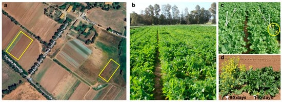
Figure 1. (a) Satellite image from Google Maps (web version Google LLC, Mountain View, CA, USA; accessed on 1 April 2024) showing the experimental fields of the BioCaramadre company (highlighted with yellow rectangles). (b) Overview of the field corresponding to the left yellow rectangle in panel (a), cultivated with a 90-day cycle genotype shown in November and photographed in January. (c) Example of a selected parcel for analysis; the yellow circle indicates plants that reached anthesis earlier than others. (d) Comparison of genotypes with different flowering times: the 90-day cycle genotype (left) versus the 140-day cycle genotype (right), both shown in November and photographed in February.

2.2. Hyperspectral Image Acquisition

Hyperspectral images of Brassica rapa subsp. sylvestris were acquired under open-field conditions at the BioCaramadre crop site (Fiumicino, Rome, Italy) using a Specim IQ camera (Specim Ltd., Oulu, Finland) working in the VIS-NIR range (400–1000 nm), a miniaturized portable device enabling in-field acquisition and real-time visualization of hyperspectral data (Figure 2) (https://www.specim.com/iq/ (accessed on 1 February 2026)). The camera operates in push-broom mode (line scanning), with a spatial resolution of 512 pixels per line and a spectral resolution of 7 nm, resulting in 204 spectral bands. Each image is square, with a resolution of 512 × 512 pixels. A built-in RGB viewfinder camera, aligned with hyperspectral optics, assists in framing and target alignment.

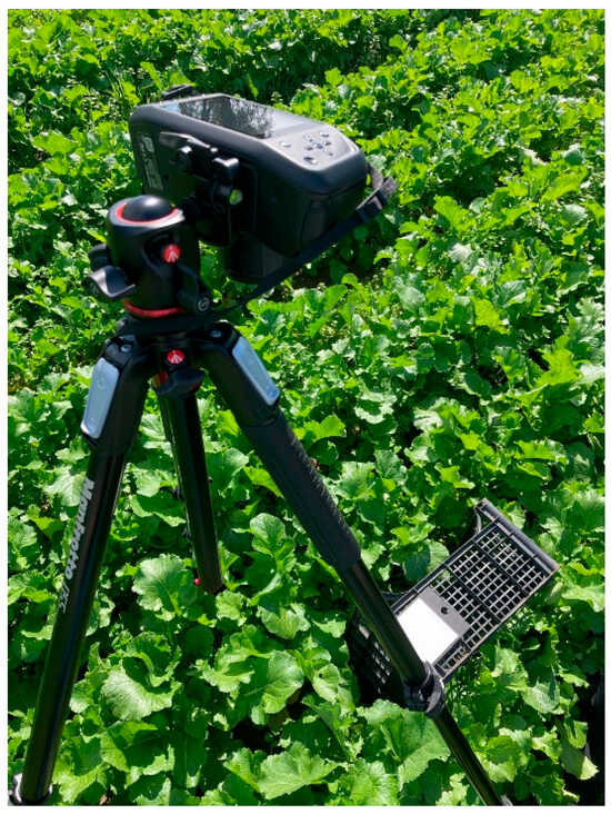
Figure 2. Specim IQ hyperspectral camera mounted on a tripod during in-field acquisition of B. rapa subsp. sylvestris.

To ensure stable data collection, the camera was mounted on a tripod (Figure 3). This stationary configuration was intentionally adopted as a proof-of-concept to validate the feasibility of the portable HSI system under real open-field conditions within a controlled field of view. The acquisition workflow included three main steps: (i) positioning and framing the target sample and the white reference at a working distance of approximately 150 cm; (ii) adjusting integration time and focus, and (iii) capturing the hyperspectral image. The Specim white reference panel (Product code: 0605221, Specim Ltd., Oulu, Finland) was positioned adjacent to each target within the scene to enable radiometric correction.

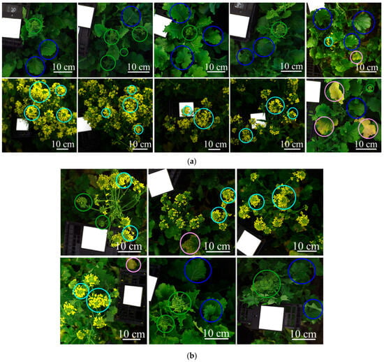
Figure 3. Sixteen source images were used to define the training and validation mosaic datasets of the classification model: (a) ten images for the training and (b) six images for the validation. Colored circles highlight representative examples of the target structures: green circles = green inflorescences; blue circles = green leaves; light blue circles = yellow flowers; pink circles = yellow leaves. Each image contains the Specim white reference panel (Product code: 0605221, Specim Ltd., Oulu, Finland).

All images were exported in reflectance mode and normalized using reference white and dark-camera images, scaling pixel values from 0 (no reflectance, dark reference) to 1 (maximum reflectance, white reference).

The acquired hyperspectral images were used to build the training (ten hyperspectral images) and validation datasets (six hyperspectral images), as shown in Figure 3. These datasets were constructed to develop and test the classification model, which was designed to identify the target plant structures—labeled as follows: green inflorescences, green leaves, yellow flowers, and yellow leaves (representative examples are highlighted with colored circles in Figure 3). The images were selected from field campaigns to be representative of the main sources of spectral variability observed under real field conditions and to support the development of an operational chemometric HSI workflow consistent with the target classes considered in this study. Furthermore, the training and validation datasets were each merged into a single mosaic to obtain representative pixel populations for all target classes. In this context, green inflorescences refer to the apical portion of the plant containing closed buds, corresponding to the stage before anthesis; green leaves indicate fully expanded photosynthetically active leaves; yellow flowers correspond to open inflorescences at anthesis, and yellow leaves represent senescent tissues showing visible chlorosis.

2.3. Hyperspectral Data Processing

Hyperspectral data processing was carried out in the MATLAB^® environment (version R2024b, The MathWorks Inc., Natick, MA, USA) using two software tools. Spectral smile correction and radiometric normalization of the hyperspectral images (Section 2.3.1) were implemented through the Hyperspectral Imaging Library for the Image Processing Toolbox™ of MATLAB^®. Subsequent chemometric preprocessing, exploratory data analysis, and classification model development were performed using the PLS_Toolbox (version 9.3, Eigenvector Research Inc.) integrated within MATLAB^®.

2.3.1. Spectral Smile and Radiometric Corrections

To account for variable illumination conditions during field acquisitions, hyperspectral data were preprocessed through a dedicated workflow based on spectral smile and radiometric corrections, aimed at minimizing spectral distortions and ensuring comparability among images [34,35,36,37,38,39,40].

Spectral smile correction was used to realign spectra along the across-track dimension, ensuring that each spatial column corresponds to a consistent wavelength across the image width. This correction reduced band misregistration and mitigated sensor-induced spectral variability [34,35,36,37,38].

Flat-field radiometric correction was applied to normalize the hyperspectral data cube [39,40]. This procedure included: (i) dark current subtraction, based on the mean dark spectrum recorded from masked or unilluminated pixels, and (ii) white reference normalization, in which a homogeneous region of interest (ROI) was selected on a Specim white reference panel (Product code: 0605221, Specim Ltd., Oulu, Finland) acquired under the same conditions; its mean spectrum was computed, and each pixel of the hyperspectral cube was divided by this mean reference spectrum. Negative values resulting from dark subtraction were set to zero to preserve physical consistency in reflectance units [39,40].

All hyperspectral images were reflectance-calibrated using a single Specim white reference panel acquired at the beginning of each acquisition session. Additional white reference measurements collected during the session served exclusively as quality checks to verify the temporal stability of illumination and sensor response.

2.3.2. Hierarchical Classification Model Building

Following the spectral smile and radiometric corrections, the hyperspectral spectra were subjected to chemometric preprocessing to enhance diagnostically meaningful spectral features and improve the robustness and generalizability of the classification model. The preprocessing strategies adopted in this study are widely used in HSI investigations coupled with multivariate analysis, particularly when dealing with complex field-acquired data affected by scattering, baseline drift, and noise [41,42,43,44,45,46,47]. Accordingly, the following set of standard preprocessing algorithms was applied:

• Detrend: a low-order polynomial was fitted to the entire spectrum of each pixel and subsequently subtracted to remove constant or linear offsets associated with background interference [44].
• Standard Normal Variate (SNV): each spectrum was mean-centered and scaled by its own standard deviation computed across all variables of that sample, giving each spectrum unit variance. This procedure acts as a zero-order detrend and mitigates scattering and multiplicative effects. SNV is a weighted normalization in which spectral points that deviate more from the sample mean contribute more strongly to the scaling [45].
• Gap Derivative: computed a gap–segment derivative in which differences were taken between two moving windows (segments) of adjacent variables separated by a fixed gap, rather than between single neighboring points. The filter is defined by the derivative order, segment size, and gap size, and operates as a linear convolution filter that attenuates low-frequency baseline variations while enhancing local spectral features [46].
• Derivative (Savitzky–Golay): derivatives were applied as a high-pass filtering operation to attenuate smooth, low-frequency baseline components and emphasize sharper, high-frequency spectral features related to chemical information. A Savitzky–Golay algorithm was used to compute the derivative while simultaneously smoothing the spectra, thereby limiting noise amplification. The method assumes that adjacent variables are strongly correlated and preserves linear relationships within the data [44].
• Mean Centering (MC): each spectral variable (column) was centered by subtracting its mean across all samples, resulting in a data matrix with zero-mean columns. This step facilitates multivariate modeling by placing all variables on a common scale around zero [47].

Principal Component Analysis (PCA) was then applied as an exploratory tool to investigate the structure of the preprocessed hyperspectral data. PCA decomposes the processed spectral data into several principal components (PCs), which are linear combinations of the original variables, reviewing spectral variability [48].

PCA score plots were used to visualize the distribution of samples (pixels) in the reduced multivariate space and to identify grouping patterns. PCA loading plots were examined to interpret the spectral variables (wavelengths) most responsible for the observed variability. These analyses enabled an assessment of the overall spectral structure of the data and the design of a hierarchical classification strategy.

Based on the PCA observations, the classification problem was decomposed into sequential decision rules, progressively addressing more challenging class separations at subsequent levels. This hierarchical decomposition was driven by the variance detected by PCA and subsequently modeled in terms of class feature covariance through PLS-DA. In this way, the original multiclass problem was organized into a dendrogram-like hierarchy, particularly suited to complex datasets in which some classes share similar spectral signatures [49]. Accordingly, a sequence of four classification models was developed to implement the hierarchical strategy, with each model built using Partial Least Squares–Discriminant Analysis (PLS-DA). PLS-DA is a linear classification method combining the regression capabilities of PLS with the discriminative power of classification techniques. It projects the original spectral variables onto a set of latent variables (LVs), which capture the most relevant sources of variability for class discrimination. This also enables graphical visualization and interpretation of data patterns and relationships through LV scores and loadings [50].

The hierarchical classification model based on PLS-DA (Hi-PLS-DA) was designed to identify six classes: (1) background, (2) green inflorescences, (3) green leaves, (4) yellow flowers, (5) yellow leaves, and (6) an additional class labeled NC (Not Classified). The NC class was assigned when a sample did not fall within any predefined class, typically due to exceeding threshold values for Q-residuals or Hotelling’s T-squared (T²) statistic [51]. To evaluate the model complexity and to select the proper number of LVs, each PLS-DA model was cross-validated using the Contiguous Block method with a window of 10 splits [52,53].

The performance of the Hi-PLS-DA model was evaluated using prediction maps and pixel-level statistical metrics. Sensitivity and specificity were calculated for both calibration and cross-validation phases, whereas sensitivity, specificity, precision, and F1-score were computed for the independent prediction phase. Both training and validation mosaic datasets were class-balanced for statistical purposes by randomly sampling an equal number of pixels per class, corresponding to the least represented class.

In terms of predicted maps, the performance of the Hi-PLS-DA model was visually evaluated by comparing the validation dataset with the corresponding ground-truth. For improved visualization and to reflect the real operational scenario, the visual comparison was reported according to the six original hyperspectral images (each image: 512 × 512 pixels) of the validation mosaic dataset.

Sensitivity (Equation (1)) refers to the model’s capability to correctly identify positive cases (i.e., the proportion of true positives among all actual positives) [54]. Specificity (Equation (2)) refers to the model’s ability to correctly identify negative cases (i.e., the proportion of true negatives among all actual negatives), thereby rejecting samples belonging to other classes [54]. Precision (Equation (3)) quantifies the proportion of correctly classified positive samples among all samples predicted as positive by the model [54]. F1-score (Equation (4)) represents the harmonic mean between precision and sensitivity, combining both metrics into a single index that accounts for false positives and false negatives. This metric is particularly informative in the presence of class imbalance, as it provides a more balanced evaluation of classification performance [54,55]. These statistical metrics range from 0 to 1, where 1 corresponds to the ideal value [55].

$$\mathrm{S}\mathrm{e}\mathrm{n}\mathrm{s}\mathrm{i}\mathrm{t}\mathrm{i}\mathrm{v}\mathrm{i}\mathrm{t}\mathrm{y}={\displaystyle \frac{\mathrm{T}\mathrm{P}}{\mathrm{T}\mathrm{P}+\mathrm{F}\mathrm{N}}}$$

(1)

$$\mathrm{S}\mathrm{p}\mathrm{e}\mathrm{c}\mathrm{i}\mathrm{f}\mathrm{i}\mathrm{c}\mathrm{i}\mathrm{t}\mathrm{y}={\displaystyle \frac{\mathrm{T}\mathrm{N}}{\mathrm{T}\mathrm{N}+\mathrm{F}\mathrm{P}}}$$

(2)

$$\mathrm{P}\mathrm{r}\mathrm{e}\mathrm{c}\mathrm{i}\mathrm{s}\mathrm{i}\mathrm{o}\mathrm{n}={\displaystyle \frac{\mathrm{T}\mathrm{P}}{\mathrm{T}\mathrm{P}+\mathrm{F}\mathrm{P}}}$$

(3)

$$\mathrm{F}1-\mathrm{s}\mathrm{c}\mathrm{o}\mathrm{r}\mathrm{e}={\displaystyle \frac{2\mathrm{T}\mathrm{P}}{2\mathrm{T}\mathrm{P}+\mathrm{F}\mathrm{P}+\mathrm{F}\mathrm{N}}}$$

(4)

where TP are true positives, TN are true negatives, FP are false positives, and FN are false negatives.

3. Results

3.1. Spectral Features and Explorative Analysis

Figure 4a shows the hyperspectral mosaic that constitutes the training dataset (the corresponding source images are shown in Figure 3a), comprising a total of 2,621,440 pixels, divided into components as follows: 641,249 pixels of the Background class; 75,062 pixels of the Green inflorescences; 1,630,375 pixels of the Green leaves; 245,729 pixels of the Yellow flowers class; 29,025 pixels of the Yellow leaves class. Figure 4b shows the corresponding average raw reflectance spectra. Figure 4c,d display the PCA score and loading plots, which are useful for exploring spectral variability among the classes studied. As shown in Figure 4b, the VIS-NIR range offers key spectral information for characterizing the target plant structures. The background class, representing a combination of non-target elements such as shadows, soil, and the white reference panel, exhibited a spectral signature with no marked features and only a modest increase in reflectance approaching 900 nm. Both green inflorescences and green leaves displayed reflectance minima around 450 nm and 680 nm, corresponding to chlorophyll absorption, followed by a sharp red-edge transition between 680 nm and 750 nm and a high NIR plateau from 750 nm to 900 nm [56,57]. Green leaves maintained stable reflectance values beyond 900 nm. Meanwhile, green inflorescences showed slightly higher overall reflectance but a decline after 900 nm, a pattern attributed to reduced intercellular spaces compared with leaf mesophyll, which decreases multiple scattering [58]. This structural compactness of sepal tissues, closer to stem-like morphology than to leaf mesophyll, likely explains the lower near-infrared scattering and provides the spectral basis to distinguish green inflorescences from green leaves despite their similar chlorophyll content. The yellow flowers’ spectrum was characterized by reduced absorption in the red region, consistent with the absence of chlorophyll and a broad absorption in the blue–green region (around 450–480 nm) associated with carotenoids, which dominate the spectral signature of yellow petals [59,60,61]. Yellow leaves, in contrast, showed spectral features linked to chlorophyll breakdown, cell wall collapse, and reduced water content, resulting in lower near-infrared reflectance and a slight blue shift in the red edge compared with yellow flowers [62,63].

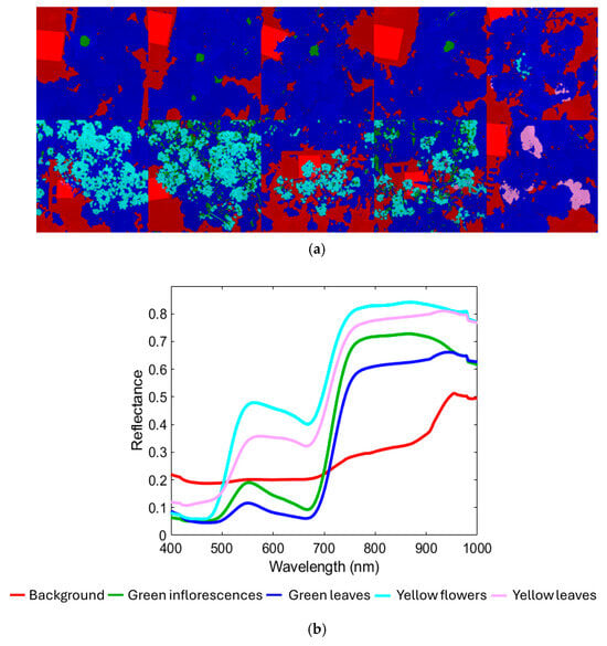
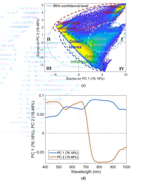
Figure 4. (a) Training dataset with classes (background, green inflorescences, green leaves, yellow flowers, and yellow leaves) and the corresponding: (b) average raw reflectance spectra in the VIS-NIR range (400–1000 nm), (c) PCA score, and (d) loadings plots.

The PCA score plot (Figure 4c) showed that most of the variance was captured by the first two PCs, where PC1 and PC2 explained 76.18% and 19.48% of the total variance, respectively. The score plot revealed a clear separation between three main clusters: (i) background; (ii) green inflorescence + green leaves; (iii) yellow flowers + yellow leaves. Furthermore, the background class formed two distinct clusters: (i) white reference mainly distributed in the first (I) quadrant; (ii) dark background elements (e.g., shadows and soil) mainly concentrated in the second (II) quadrant. Green inflorescences and green leaves classes were mostly located in the central region of the plot, spanning the second (II), third (III), and fourth (IV) quadrants. Yellow flowers and yellow leaves classes were mainly positioned between the first (I) and fourth (IV) quadrants.

The corresponding loading plots (Figure 4d) indicated that PC1 was mainly associated with spectral regions of 450 and 680 nm, reflecting the predominance of chlorophyll-related features, and with a high reflectance plateau from 720 nm to 900 nm. PC2 showed strong contributions in the 680–750 nm range, likely related to variability in the red-edge transition. The patterns observed in the score and loading plots explained the partial separation of yellow tissues (yellow leaves and yellow flowers) from green tissues (green inflorescences and green leaves), as senescent or floral tissues typically exhibit a blue shift in the red edge compared with chlorophyll-rich tissues [56,57]. However, classes dominated by the same pigments (e.g., chlorophyll-rich tissues: green leaves vs. green inflorescences; carotenoid-rich tissues: yellow leaves vs. yellow flowers) exhibited similar spectral signatures, leading to overlap in the score plot.

Overall, these observations suggested that a hierarchical classification structure based on progressive spectral separability could be organized as follows: an initial separation between background and plant tissues, followed by a progressive refinement first between green and yellow tissues, and then between spectrally similar subclasses (green inflorescences vs. green leaves, and yellow flowers vs. yellow leaves).

3.2. Hi-PLS-DA Model Building Results

Starting with the pattern observed during exploratory analysis with PCA, a total of four sequential decision rules were developed and assembled to form the Hi-PLS-DA model. Each rule corresponded to a distinct PLS-DA model, differing in preprocessing strategy and LVs, as summarized below:

• Rule 1, developed with three LVs, applied MC as a preprocessing method and produced three outputs: (1) background; (2) green inflorescences, green leaves, yellow flowers, yellow leaves; (3) NC.
• Rule 2, based on three LVs and built using SNV, second derivative (order 2, window 21 points), and MC, generating three outputs: (1) green inflorescences and green leaves; (2) yellow flowers and yellow leaves; (3) NC.
• Rule 3, constructed with three LVs, was built using SNV, first derivative (order 2, window 17 points, weighted tails), and MC, and produced three outputs: (1) green inflorescences; (2) green leaves; (3) NC.
• Rule 4, developed with three LVs, involved SNV, second derivative (order 2, window 9 points, including only weighted tails), and MC, providing three outputs: (1) yellow flowers; (2) yellow leaves; (3) NC.

The sequence of decision rules reflects the progressive spectral separability observed with PCA, where an initial separation distinguished background from plant structures (Rule 1), followed by a discrimination between green and yellow tissues (Rule 2). At deeper levels of the hierarchy, increasingly spectrally similar subclasses were resolved, first separating green inflorescences from green leaves (Rule 3) and then yellow flowers from yellow leaves (Rule 4).

Figure 5 illustrates the outcome of combining the four decision rules (i.e., four PLS-DA models), showing the dendrogram structure of the Hi-PLS-DA model.

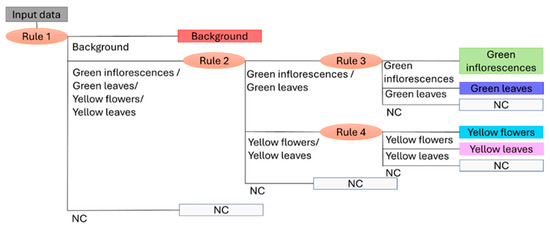
Figure 5. Dendrogram structure of the Hi-PLS-DA model built by assembling 4 rules and utilized to classify the target classes: background, green inflorescences, green leaves, yellow flowers, yellow leaves, and NC (Not Classified).

3.3. Hi-PLS-DA Results

Figure 6a–r displays the classification results for the validation dataset, presented as individual images corresponding to the six original hyperspectral acquisitions (each image: 512 × 512 pixels) composing the validation mosaic dataset. For each hyperspectral images, the source image (Figure 6a,d,g,j,m,p), the corresponding expected (ground-truth) class map (Figure 6b,e,h,k,n,q) and predicted class map (Figure 6c,f,i,l,o,r) are reported, allowing a direct visual comparison between the expected and predicted outcomes.

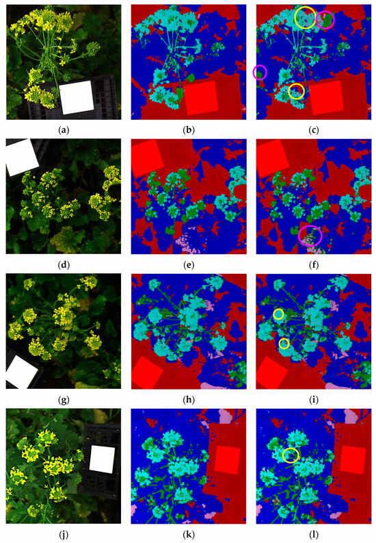
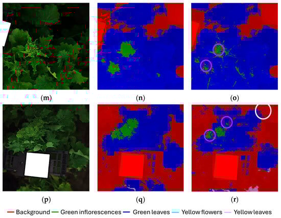
Figure 6. Classification results of the validation dataset, shown separately for each original hyperspectral acquisition: (a,d,g,j,m,p) source images, (b,e,h,k,n,q) expected (ground-truth) class maps and (c,f,i,l,o,r) predicted maps obtained using the Hi-PLS-DA model. Colored circles, highlighted in the predicted maps, indicate representative examples of misclassifications: yellow circles = yellow flower pixels misclassified as yellow leaves; purple circles = green leaf pixels misclassified as green inflorescences; white circles = green leaf pixels misclassified as background.

The model was able to correctly identify the presence of harvestable inflorescences within the field scene, demonstrating the robustness of the hierarchical strategy in addressing this critical task. The green inflorescences showed the highest degree of confusion with green leaves. This can be attributed to both classes being dominated by chlorophyll and exhibiting very similar reflectance features in the 400–1000 nm range. From a biological perspective, immature inflorescences are externally formed by green sepals, which are morphologically and biochemically very similar to leaves, thus contributing to their spectral overlap. In contrast, yellow flowers were easily identified and only minimally confused with yellow leaves. This separability can be attributed to the distinct reflectance patterns of floral tissues dominated by carotenoids compared with senescent leaves, which combine carotenoid dominance with structural degradation and water loss. Some residual confusion was observed between green leaves and the background class. This can be explained by the heterogeneity of the background, which included not only soil and the white reference panel, but also shaded leaves partially occluded by other plant structures. To further support results interpretation, selected misclassifications are highlighted in the predicted maps, as follows:

• Figure 6c,i,l: yellow circles indicate examples of yellow flower pixels misclassified as yellow leaves.
• Figure 6c,f,o,r: purple circles indicate examples of green leaf pixels misclassified as green inflorescences.
• Figure 6r: white circle highlights indicate examples of green leaf pixels misclassified as background.

The sensitivity and specificity values of the model for the calibration and cross-validation phases are reported in Table 1, showing high performance metrics ranging from 0.84 to 0.99. These results refer to calibration and cross-validation performances computed on the class-balanced training mosaic dataset, with 29,025 pixels per class, corresponding to the least represented class (i.e., Yellow leaves class).

Table 1. Sensitivity and specificity values in calibration (Cal) and cross-validation (CV) phases, for each rule of the Hi-PLS-DA model.

Rules	Classes	Background	Green inflorescences + Green leaves + Yellow flowers + Yellow leaves
Rule 1	Sensitivity (Cal)	0.99	0.97
	Specificity (Cal)	0.97	0.99
	Sensitivity (CV)	0.99	0.97
	Specificity (CV)	0.97	0.99
Rule 2	Classes	Green inflorescences + Green leaves	Yellow flowers + Yellow leaves
	Sensitivity (Cal)	0.97	0.99
	Specificity (Cal)	0.99	0.97
	Sensitivity (CV)	0.96	0.99
	Specificity (CV)	0.99	0.96
Rule 3	Classes	Yellow flowers	Yellow leaves
	Sensitivity (Cal)	0.94	0.90
	Specificity (Cal)	0.90	0.94
	Sensitivity (CV)	0.84	0.91
	Specificity (CV)	0.91	0.84
Rule 4	Classes	Green inflorescences	Green leaves
	Sensitivity (Cal)	0.91	0.91
	Specificity (Cal)	0.91	0.91
	Sensitivity (CV)	0.90	0.90
	Specificity (CV)	0.90	0.90

Rule 1, separating background from all vegetation classes, achieved the highest values (sensitivity and specificity >0.97), confirming the robustness of the model in excluding non-target elements. Rule 2, distinguishing green tissues (green inflorescences + green leaves) from yellow tissues (yellow flowers + yellow leaves), also performed very well, with sensitivity and specificity values above 0.96 in both calibration and cross-validation. Rule 3, separating yellow flowers from yellow leaves, showed slightly lower performance (sensitivity ranging from 0.84 to 0.94), reflecting the strong spectral similarity between these two classes. Finally, Rule 4, discriminating green inflorescences from green leaves, also achieved balanced values (around 0.90–0.91), indicating that the model was able to capture subtle spectral differences between these chlorophyll-rich tissues.

The sensitivity, specificity, precision, and F1-score values of the Hi-PLS-DA model for the prediction phase are reported in Table 2, showing performance metrics ranging from 0.78 to 1.00. These results refer to prediction performances computed on the class-balanced validation mosaic dataset, with 2708 pixels per class, corresponding to the least represented class (i.e., Yellow leaves class). The lowest value was observed for the green inflorescences class, consistent with the misclassifications identified in the predicted HSI maps and explained by its spectral similarity to the green leaves class. All other classes achieved sensitivity and specificity values above 0.87, confirming the robustness of the hierarchical model.

Table 2. Statistical metrics values in the prediction phase (Pred) of the Hi-PLS-DA model.

Class	Sensitivity (Pred)	Specificity (Pred)	Precision	F1-Score
Background	0.99	0.95	0.96	0.98
Green inflorescences	0.78	0.99	0.84	0.80
Green leaves	0.93	0.97	0.93	0.92
Yellow flowers	0.93	1.00	0.93	0.92
Yellow leaves	0.87	0.99	0.79	0.86

In summary, while classes dominated by different pigments (chlorophyll vs. carotenoids) were effectively separated, some misclassification remained between classes sharing similar biochemical and structural features. Despite these challenges, the model successfully captured the essential agronomic information by accurately discriminating harvestable (non-flowering) from non-harvestable (flowering) plants under real field conditions.

4. Discussion

Recent literature shows that hyperspectral and spectroscopic approaches are increasingly being explored to support selective harvesting and agricultural decision-making processes with different specific objectives, sensors, and data-processing strategies [64,65,66,67,68,69]. In fruit crops, Ma et al. [64] developed a portable, field-deployable VIS–NIR spatially resolved spectroscopic (SRS) system for kiwifruit to estimate firmness and soluble solids content directly in the orchard, demonstrating that portable optical sensing can support “time-to-harvest” decisions under real-field conditions. This work highlights both the feasibility and the practical challenges of in situ spectral measurements, particularly the influence of skin properties and light scattering on prediction accuracy.

Similarly, Tsakiridis et al. [65] applied in situ VIS-NIR HSI on grapes, proposing deep autoencoders to compensate for variable illumination in open-field conditions before estimating sugar content. This study underscores that illumination variability, shadowing, and canopy geometry are key limiting factors for field HSI, and that advanced data normalization strategies may be required to mitigate these effects before quantitative modeling. Moreover, the authors explicitly discuss the future mounting of hyperspectral cameras on mobile or robotic platforms, highlighting the transition from stationary to mobile sensing as a key research frontier.

In Brassica crops, Guo et al. [66] used HSI combined with spectral unmixing and machine learning to monitor glucosinolate dynamics and early senescence in stored broccoli. This confirms the capacity of HSI to capture subtle biochemical changes in Brassica tissues, but it remains laboratory-based and postharvest.

Recent systematic reviews further emphasize that the field is moving toward real-time, embedded hyperspectral analysis, although only a limited number of ground-based systems currently achieve true operational deployment [27,67,68]. Building on these advances, the present study provides a practical basis for using a portable VIS–NIR HSI system directly in the field to support harvest-timing decisions in Brassica rapa subsp. sylvestris. In contrast to many previous studies that were either laboratory-based or focused mainly on biochemical traits, this work offers an operational, ground-based pathway from raw field acquisitions to actionable harvest maps under open-field conditions.

While deep-learning approaches are gaining traction, their practical deployment in real agricultural environments can still be constrained by data availability and computational requirements [16,67,68]. In this context, the hierarchical classification strategy represents a pragmatic and transferable alternative under current technological conditions, relying on PLS-DA as a well-established chemometric method valued for its interpretability and robustness in applied hyperspectral studies [69]. By integrating dedicated spectral preprocessing with this interpretable hierarchical PLS-DA strategy, pixel-by-pixel mapping of pre- and post-anthesis plants was achieved under real environmental conditions. Therefore, the resulting maps support data-driven monitoring and decision-making for precision harvesting and pave the way for possible future integration with automated mobile platforms, including ground-based vehicles or unmanned aerial systems, which have been increasingly explored in recent work on operational HSI in field environments [16,27].

5. Conclusions

In this study, a hierarchical classification workflow based on a portable HSI system in the VIS–NIR range (400–1000 nm) was developed and applied under real field conditions to discriminate harvestable (pre-anthesis) and non-harvestable (post-anthesis) plants. Using Brassica rapa subsp. sylvestris as a case study, the approach demonstrated reliable prediction performance and robustness to spectral variability typically encountered in outdoor HSI data. The proposed model achieved satisfactory prediction results, with performance metrics (sensitivity, specificity, precision, and F1-score) values ranging from 0.78 to 1.00 across classes and consistent classification maps despite challenges, such as changing illumination and heterogeneous canopy structure. The hierarchical model successfully identified the target plant structures, green inflorescences, green leaves, yellow flowers, and yellow leaves, demonstrating its ability to resolve even subtle spectral differences between plant tissues. The most frequent misclassifications occurred between green inflorescences and green leaves due to their similar chemical composition, while flower structures (yellow flower class) were recognized more accurately, supporting their relevance in harvesting decisions. Despite the presence of confounding factors such as wind-induced movement, partial occlusions, and background variability, the proposed workflow provided stable discrimination of flowering and non-flowering tissues at the canopy level, highlighting its applicability for in situ monitoring and selective harvesting.

Beyond this specific crop, the proposed workflow illustrates how hierarchical modeling can effectively address complex classification challenges where plant organs exhibit very similar spectral signatures that are difficult to distinguish. A key advantage of the hierarchical design is its modularity, which allows new classes or operational conditions (e.g., additional plant organs, stress conditions, or contaminants) to be incorporated as new nodes without redesigning the entire model. The same analytical methodology can be implemented for other vegetable crops with comparable flowering dynamics, supporting precise phenological monitoring and optimal harvest scheduling. Although the portable HSI system was used in the field in a stationary configuration in this study, the proposed workflow is potentially transferable to the same sensing technology mounted on mobile platforms operating. Its compatibility with portable HSI systems further highlights its potential for future integration into automated field platforms, enabling continuous field monitoring or selective harvesting based on user-defined operational thresholds. To further consolidate the general applicability of the proposed workflow under diverse operational conditions, future work may progressively integrate additional field sites and cropping seasons within the same modular and updatable framework.

References

- Franks, S.J.; Sim, S.; Weis, A.E. Rapid evolution of flowering time by an annual plant in response to a climate fluctuation. Proc. Natl. Acad. Sci. USA 2007, 104, 1278–1282. [Google Scholar] [CrossRef] [PubMed]
- Islam, M.; Bijjahalli, S.; Fahey, T.; Gardi, A.; Sabatini, R.; Lamb, D.W. Destructive and non-destructive measurement approaches and the application of AI models in precision agriculture: A review. Precis. Agric. 2024, 25, 1127–1180. [Google Scholar] [CrossRef]
- Piao, S.; Liu, Q.; Chen, A.; Janssens, I.A.; Fu, Y.; Dai, J.; Liu, L.; Lian, X.; Shen, M.; Zhu, X. Plant phenology and global climate change: Current progresses and challenges. Glob. Change Biol. 2019, 25, 1922–1940. [Google Scholar] [CrossRef]
- Arangurí, M.; Mera, H.; Noblecilla, W.; Lucini, C. Digital literacy and technology adoption in agriculture: A systematic review of factors and strategies. AgriEngineering 2025, 7, 296. [Google Scholar] [CrossRef]
- Kumari, K.; Mirzakhani Nafchi, A.; Mirzaee, S.; Abdalla, A. AI-driven future farming: Achieving climate-smart and sustainable agriculture. AgriEngineering 2025, 7, 89. [Google Scholar] [CrossRef]
- Kior, A.; Yudina, L.; Zolin, Y.; Sukhov, V.; Sukhova, E. RGB imaging as a tool for remote sensing of characteristics of terrestrial plants: A review. Plants 2024, 13, 1262. [Google Scholar] [CrossRef]
- Song, P.; Li, Z.; Yang, M.; Shao, Y.; Pu, Z.; Yang, W.; Zhai, R. Dynamic detection of three-dimensional crop phenotypes based on a consumer-grade RGB-D camera. Front. Plant Sci. 2023, 14, 1097725. [Google Scholar] [CrossRef]
- Thai, T.; Mansoor, S.; Le, A.; Baloch, F.; Chung, Y.; Dong-Wook, K. Limitation of RGB-Derived Vegetation Indices Using UAV Imagery for Biomass Estimation during Buckwheat Flowering. Phyton 2025, 94, 2215. [Google Scholar] [CrossRef]
- Kendal, D.; Hauser, C.E.; Garrard, G.E.; Jellinek, S.; Giljohann, K.M.; Moore, J.L. Quantifying plant colour and colour difference as perceived by humans using digital images. PLoS ONE 2013, 8, e72296. [Google Scholar] [CrossRef]
- Huang, Q.; Yang, M.; Ouyang, L.; Wang, Z.; Lin, J. VIS/NIR spectroscopy and chemometrics for non-destructive estimation of chlorophyll content in different plant leaves. Sensors 2025, 25, 1673. [Google Scholar] [CrossRef] [PubMed]
- Cattaneo, T.M.; Stellari, A. NIR Spectroscopy as a Suitable Tool for the Investigation of the Horticultural Field. Agronomy 2019, 9, 503. [Google Scholar] [CrossRef]
- Schuh, S.; Czerny, B. Spectral reflectance analysis of plant leaves during accelerated senescence in the VIS, NIR, MIR range. In Integrated Optics: Design, Devices, Systems and Applications VII; SPIE: Bellingham, WA, USA, 2023; Volume 12575, pp. 93–98. [Google Scholar]
- Devadas, R.; Lamb, D.W.; Simpfendorfer, S.; Backhouse, D. Evaluating ten spectral vegetation indices for identifying rust infection in individual wheat leaves. Precis. Agric. 2009, 10, 459–470. [Google Scholar] [CrossRef]
- Tripodi, P.; Massa, D.; Venezia, A.; Cardi, T. Sensing technologies for precision phenotyping in vegetable crops: Current status and future challenges. Agronomy 2018, 8, 57. [Google Scholar] [CrossRef]
- Sarić, R.; Nguyen, V.D.; Burge, T.; Berkowitz, O.; Trtílek, M.; Whelan, J.; Lewsey, M.G.; Čustović, E. Applications of hyperspectral imaging in plant phenotyping. Trends Plant Sci. 2022, 27, 301–315. [Google Scholar] [CrossRef]
- Lu, B.; Dao, P.D.; Liu, J.; He, Y.; Shang, J. Recent advances of hyperspectral imaging technology and applications in agriculture. Remote Sens. 2020, 12, 2659. [Google Scholar] [CrossRef]
- Patel, D.; Bhise, S.; Kapdi, S.S.; Bhatt, T. Non-destructive hyperspectral imaging technology to assess the quality and safety of food: A review. Food Prod. Process. Nutr. 2024, 6, 69. [Google Scholar] [CrossRef]
- Adesokan, M.; Alamu, E.O.; Otegbayo, B.; Maziya-Dixon, B. A review of the use of near-infrared hyperspectral imaging (NIR-HSI) techniques for the non-destructive quality assessment of root and tuber crops. Appl. Sci. 2023, 13, 5226. [Google Scholar] [CrossRef]
- Castro-Valdecantos, P.; Egea, G.; Borrero, C.; Pérez-Ruiz, M.; Avilés, M. Detection of Fusarium wilt-induced physiological impairment in strawberry plants using hyperspectral imaging and machine learning. Precis. Agric. 2024, 25, 2958–2976. [Google Scholar] [CrossRef]
- Li, L.; Jia, X.; Fan, K. Recent advance in nondestructive imaging technology for detecting quality of fruits and vegetables: A review. Crit. Rev. Food Sci. Nutr. 2025, 65, 5181–5199. [Google Scholar] [CrossRef]
- Lee, W.S.; Alchanatis, V.; Yang, C.; Hirafuji, M.; Moshou, D.; Li, C. Sensing technologies for precision specialty crop production. Comput. Electron. Agric. 2010, 74, 2–33. [Google Scholar] [CrossRef]
- Jia, W.; Pang, Y.; Tortini, R. The influence of BRDF effects and representativeness of training data on tree species classification using multi-flightline airborne hyperspectral imagery. ISPRS J. Photogramm. Remote Sens. 2024, 207, 245–263. [Google Scholar] [CrossRef]
- Amigo, J.M.; Martí, I.; Gowen, A. Hyperspectral imaging and chemometrics: A perfect combination for the analysis of food structure, composition and quality. In Data Handling in Science and Technology; Elsevier: Amsterdam, The Netherlands, 2013; Volume 28, pp. 343–370. [Google Scholar] [CrossRef]
- Amigo, J.M.; Babamoradi, H.; Elcoroaristizabal, S. Hyperspectral image analysis: A tutorial. Anal. Chim. Acta 2015, 896, 34–51. [Google Scholar] [CrossRef]
- Biancolillo, A.; Marini, F.; Ruckebusch, C.; Vitale, R. Chemometric strategies for spectroscopy-based food authentication. Appl. Sci. 2020, 10, 6544. [Google Scholar] [CrossRef]
- Calvini, R.; Ulrici, A.; Marini, F. Hyperspectral imaging and multivariate analysis for food quality assessment. Compr. Anal. Chem. 2021, 94, 275–314. [Google Scholar] [CrossRef]
- Ram, B.G.; Oduor, P.; Igathinathane, C.; Howatt, K.; Sun, X. A systematic review of hyperspectral imaging in precision agriculture: Analysis of its current state and future prospects. Comput. Electron. Agric. 2024, 222, 109037. [Google Scholar] [CrossRef]
- Conversa, G.; Bonasia, A.; Lazzizera, C.; Elia, A. Bio-physical, physiological, and nutritional aspects of ready-to-use cima di rapa (Brassica rapa L. subsp. sylvestris L. Janch. var. esculenta Hort.) as affected by conventional and organic growing systems and storage time. Sci. Hortic. 2016, 213, 76–86. [Google Scholar] [CrossRef]
- Luo, F.; Fang, H.; Wei, B.; Cheng, S.; Zhou, Q.; Zhou, X.; Zhan, X.; Zhao, Y.; Ji, S. Advances in yellowing mechanisms and regulation technology of post-harvested broccoli. Food Qual. Saf. 2020, 4, 107–113. [Google Scholar] [CrossRef]
- de Chiara, M.L.V.; Cefola, M.; Pace, B.; Palumbo, M.; Amodio, M.L.; Colelli, G. Ready-to-use broccoli raab (Brassica rapa L. subsp. sylvestris) quality and volatilome as affected by packaging. Postharvest Biol. Technol. 2024, 213, 112961. [Google Scholar] [CrossRef]
- Kitić, G.; Tagarakis, A.; Cselyuszka, N.; Panić, M.; Birgermajer, S.; Sakulski, D.; Matović, J. A new low-cost portable multispectral optical device for precise plant status assessment. Comput. Electron. Agric. 2019, 162, 300–308. [Google Scholar] [CrossRef]
- Mäkelä, M.; Geladi, P.; Rissanen, M.; Rautkari, L.; Dahl, O. Hyperspectral near infrared image calibration and regression. Anal. Chim. Acta 2020, 1105, 56–63. [Google Scholar] [CrossRef]
- Testone, G.; Sobolev, A.P.; Lambreva, M.D.; Aturki, Z.; Mele, G.; Lamprillo, M.; Magnanimi, F.; Serino, G.; Arnesi, G.; Giannino, D. The molecular pathways leading to GABA and lactic acid accumulation in florets of organic broccoli rabe (Brassica rapa subsp. sylvestris) stored as fresh or as minimally processed product. Hortic. Res. 2025, 12, uhae274. [Google Scholar] [CrossRef]
- Ceamanos, X.; Douté, S. Spectral smile correction of CRISM/MRO hyperspectral images. IEEE Trans. Geosci. Remote Sens. 2010, 48, 3951–3959. [Google Scholar] [CrossRef]
- Roberts, D.A.; Yamaguchi, Y.; Lyon, R.J. Comparison of various techniques for calibration of AIS data. NASA STI/Recon Tech. Rep. N 1986, 87, 21–30. [Google Scholar]
- The MathWorks. ReduceSmile. 2025. Available online: https://it.mathworks.com/help/images/ref/reducesmile.html (accessed on 1 February 2026).
- Souri, A.H.; Sharifi, M.A. Evaluation of scene-based empirical approaches for atmospheric correction of hyperspectral imagery. In Proceedings of the 33rd Asian Conference of Remote Sensing, Pattaya, Thailand, 26–30 November 2012; Volume 26. [Google Scholar]
- Perkins, T.; Adler-Golden, S.; Matthew, M.W.; Berk, A.; Bernstein, L.S.; Lee, J.; Fox, M. Speed and accuracy improvements in FLAASH atmospheric correction of hyperspectral imagery. Opt. Eng. 2012, 51, 111707. [Google Scholar] [CrossRef]
- The MathWorks. FlatField. 2025. Available online: https://it.mathworks.com/help/images/ref/flatfield.html (accessed on 1 February 2026).
- The MathWorks. SubtractDarkPixel. 2025. Available online: https://it.mathworks.com/help/images/ref/subtractdarkpixel.html (accessed on 1 February 2026).
- Bro, R.; Smilde, A.K. Centering and scaling in component analysis. J. Chemom. 2003, 17, 16–33. [Google Scholar] [CrossRef]
- Rinnan, Å. Pre-processing in vibrational spectroscopy–when, why and how. Anal. Methods 2014, 6, 7124–7129. [Google Scholar] [CrossRef] [PubMed]
- Bonifazi, G.; Capobianco, G.; Gasbarrone, R.; Serranti, S. Contaminant detection in pistachio nuts by different classification methods applied to short-wave infrared hyperspectral images. Food Control 2021, 130, 108202. [Google Scholar] [CrossRef]
- Eigenvector Research. Advanced Preprocessing: Noise, Offset, and Baseline Filtering. 2019. Available online: https://www.eigenvectordocs.com/index.php?title=Advanced_Preprocessing:_Noise,_Offset,_and_Baseline_Filtering#Detrend (accessed on 1 February 2026).
- Eigenvector Research. Advanced Preprocessing: Sample Normalization. 2021. Available online: https://www.eigenvectordocs.com/index.php?title=Advanced_Preprocessing:_Sample_Normalization (accessed on 1 February 2026).
- Eigenvector Research. Gapsegment. 2013. Available online: https://www.eigenvectordocs.com/index.php?title=Gapsegment (accessed on 1 February 2026).
- Eigenvector Research. Mncn. 2011. Available online: https://www.eigenvectordocs.com/index.php?title=Mncn (accessed on 1 February 2026).
- Bro, R.; Smilde, A.K. Principal component analysis. Anal. Methods 2014, 6, 2812–2831. [Google Scholar] [CrossRef]
- Monakhova, Y.B.; Hohmann, M.; Christoph, N.; Wachter, H.; Rutledge, D.N. Improved classification of fused data: Synergetic effect of partial least squares discriminant analysis (PLS-DA) and common components and specific weights analysis (CCSWA) combination as applied to tomato profiles (NMR, IR and IRMS). Chemom. Intell. Lab. Syst. 2016, 156, 1–6. [Google Scholar] [CrossRef]
- Ballabio, D.; Consonni, V. Classification tools in chemistry. Part 1: Linear models. PLS-DA. Anal. Methods 2013, 5, 3790–3798. [Google Scholar] [CrossRef]
- Eigenvector Research. T-Squared Q residuals and Contributions. 2025. Available online: https://www.eigenvectordocs.com/index.php?title=T-Squared_Q_residuals_and_Contributions (accessed on 1 February 2026).
- Eigenvector Research. Plsda. 2023. Available online: https://www.eigenvectordocs.com/index.php?title=Plsda (accessed on 1 February 2026).
- Eigenvector Research. Using Cross-Validation. 2023. Available online: https://www.eigenvectordocs.com/index.php?title=Using_Cross-Validation (accessed on 1 February 2026).
- Eigenvector Research. Confusionmatrix. 2018. Available online: https://www.eigenvectordocs.com/index.php?title=Confusionmatrix (accessed on 1 February 2026).
- Lee, N.Y.; Na, I.S.; Lee, K.W.; Lee, D.H.; Kim, J.W.; Kook, M.C.; Hong, S.J.; Son, J.Y.; Lee, A.Y.; Om, A.S.; et al. Detection of physical hazards from fruit processed products using hyperspectral imaging and prediction based on PLS-DA and logistic regression machine learning models. Appl. Food Res. 2024, 4, 100506. [Google Scholar] [CrossRef]
- Gitelson, A.; Merzlyak, M.N. Spectral reflectance changes associated with autumn senescence of Aesculus hippocastanum L. and Acer platanoides L. leaves. J. Plant Physiol. 1994, 143, 286–292. [Google Scholar] [CrossRef]
- Gitelson, A.A.; Peng, Y.; Arkebauer, T.J.; Schepers, J.S. Relationship between gross primary production and chlorophyll content in crops. J. Plant Physiol. 2014, 171, 626–633. [Google Scholar] [CrossRef]
- Jacquemoud, S.; Ustin, S. Leaf Optical Properties; Cambridge University Press: Cambridge, UK, 2019. [Google Scholar] [CrossRef]
- Kay, Q.O.N.; Daoud, H.S.; Stirton, C.H. Pigment distribution, light reflection and cell structure in petals. Bot. J. Linn. Soc. 1981, 83, 57–83. [Google Scholar] [CrossRef]
- Sims, D.A.; Gamon, J.A. Relationships between leaf pigment content and spectral reflectance across a wide range of species, leaf structures and developmental stages. Remote Sens. Environ. 2002, 81, 337–354. [Google Scholar] [CrossRef]
- Ustin, S.L.; Jacquemoud, S. How the optical properties of leaves modify the absorption and scattering of energy and enhance leaf functionality. In Remote Sensing of Plant Biodiversity; Springer International Publishing: Cham, Switzerland, 2020; pp. 349–384. [Google Scholar] [CrossRef]
- Merzlyak, M.N.; Gitelson, A. Why and what for the leaves are yellow in autumn? On the interpretation of optical spectra of senescing leaves (Acerplatanoides L.). J. Plant Physiol. 1995, 145, 315–320. [Google Scholar] [CrossRef]
- Gamon, J.A.; Surfus, J.S. Assessing leaf pigment content and activity with a reflectometer. New Phytol. 1999, 143, 105–117. [Google Scholar] [CrossRef]
- Ma, T.; Inagaki, T.; Tsuchikawa, S.; Jiang, H. A field-deployable spectroscopic approach for optimizing kiwifruit harvest timing and postharvest quality management. Postharvest Biol. Technol. 2026, 231, 113888. [Google Scholar] [CrossRef]
- Tsakiridis, N.L.; Samarinas, N.; Kokkas, S.; Kalopesa, E.; Tziolas, N.V.; Zalidis, G.C. In situ grape ripeness estimation via hyperspectral imaging and deep autoencoders. Comput. Electron. Agric. 2023, 212, 108098. [Google Scholar] [CrossRef]
- Guo, X.; Ahlawat, Y.K.; Liu, T.; Zare, A. Evaluation of postharvest senescence of broccoli via hyperspectral imaging. Plant Phenomics 2022, 2022, 9761095. [Google Scholar] [CrossRef]
- Khan, A.; Vibhute, A.D.; Mali, S.; Patil, C.H. A systematic review on hyperspectral imaging technology with a machine and deep learning methodology for agricultural applications. Ecol. Inform. 2022, 69, 101678. [Google Scholar] [CrossRef]
- Shafi, U.; Mumtaz, R.; García-Nieto, J.; Hassan, S.A.; Zaidi, S.A.R.; Iqbal, N. Precision agriculture techniques and practices: From considerations to applications. Sensors 2019, 19, 3796. [Google Scholar] [CrossRef] [PubMed]
- Lee, L.C.; Liong, C.Y.; Jemain, A.A. Partial least squares-discriminant analysis (PLS-DA) for classification of high-dimensional (HD) data: A review of contemporary practice strategies and knowledge gaps. Analyst 2018, 143, 3526–3539. [Google Scholar] [CrossRef] [PubMed]
Disclaimer/Publisher’s Note: The statements, opinions and data contained in all publications are solely those of the individual author(s) and contributor(s) and not of MDPI and/or the editor(s). MDPI and/or the editor(s) disclaim responsibility for any injury to people or property resulting from any ideas, methods, instructions or products referred to in the content. |
© 2026 by the authors. Licensee MDPI, Basel, Switzerland. This article is an open access article distributed under the terms and conditions of the Creative Commons Attribution (CC BY) license.