A Hybrid Model for Multi-Day-Ahead Electricity Price Forecasting considering Price Spikes

Abstract

This paper proposes a new hybrid model to forecast electricity market prices up to four days ahead. The components of the proposed model are combined in two dimensions. First, on the “vertical” dimension, long short-term memory (LSTM) neural networks and extreme gradient boosting (XGBoost) models are stacked up to produce supplementary price forecasts. The final forecasts are then picked depending on how the predictions compare to a price spike threshold. On the “horizontal” dimension, five models are designed to extend the forecasting horizon to four days. This is an important requirement to make forecasts useful for market participants who trade energy and ancillary services multiple days ahead. The horizontally cascaded models take advantage of the availability of specific public data for each forecasting horizon. To enhance the forecasting capability of the model in dealing with price spikes, we deploy a previously unexplored input in the proposed methodology. That is, to use the recent variations in the output power of thermal units as an indicator of unplanned outages or shift in the supply stack. The proposed method is tested using data from Alberta’s electricity market, which is known for its volatility and price spikes. An economic application of the developed forecasting model is also carried out to demonstrate how several market players in the Alberta electricity market can benefit from the proposed multi-day ahead price forecasting model. The numerical results demonstrate that the proposed methodology is effective in enhancing forecasting accuracy and price spike detection.

1. Introduction

Spot prices in competitive electricity markets exhibit seasonality, volatility, and price spike occurrence [1,2,3]. The occurrence of price spikes is associated with different system events, for instance, the scheduled and forced outage of generation and transmission assets, transmission congestion, and extreme weather events leading to increased demand or shortage of supply [2,4,5]. Accurately forecasting price spikes holds paramount importance [6] due to their potential to inflict significant financial losses upon unsuspecting business owners. Moreover, traditional forecasting models encounter significant challenges in effectively accounting for and managing these volatile market conditions [7]. Even though price volatility can be observed in all power markets, real-time markets are more prone to the price risks associated with such unforeseen spikes [1]. Higher price volatility in real-time electricity markets adds to the difficulty of producing reasonably accurate electricity price forecasts [8], while forecasting errors for day-ahead markets are often reported to be single-digit, comparable studies often report significantly higher errors for real-time markets [9,10].

There are plenty of studies in the literature that have undertaken the challenge of forecasting electricity market prices. Between a very recent review [11] and one that was published in 2014 [4], the interested reader can find a comprehensive summary of applied methods, best practices, and tips and recommendations for future research in this domain. There are, however, a few observations that are worth noting in the context of the present work. First, the vast majority of available methods are applied to day-ahead market prices. This is understandable because most electricity markets have a day-ahead market component in which most of the energy is traded [3,12,13]. There are a few jurisdictions with only a real-time market mechanism, including Alberta and Ontario provinces in Canada, Australia, and New Zealand. Second, almost all available studies have limited their forecasting horizon to the next day, with a few exceptions, e.g., [14,15], that look beyond the next day. Longer forecast horizons are useful, and sometimes necessary, for optimizing operation plans and portfolio management for market participants. For example, in Alberta, participants in the ancillary services market rely on energy price forecasts generated before 1:00 p.m. on Fridays for the following Monday to optimize their portfolio [16]. Third, only a limited number of papers have taken price spikes into account when designing their models or when evaluating the performance of their proposed models. For example, ref. [5] used an auto-regressive conditional hazard model to predict the probability of one-step-ahead price spikes in the Australian electricity market. In [8], system demand forecasts along with weather information were used in a hybrid neural-network-based model to forecast next-day normal and spike prices for Ontario’s electricity market. In [17], other exogenous variables, such as reserve capacity, variable generation, and interconnection flows, were examined to predict the probability of extremely high or low prices for the next day in the Australian market.

In this paper, we propose a hybrid model to predict the real-time electricity market prices in Alberta for up to four days in advance. The model is designed particularly to handle the extended forecasting horizon and the high volatility of prices in this market caused by frequent price spikes. This is achieved through two main contributions. The first contribution is that the proposed hybrid model combines multiple models at two dimensions. More specifically, at a “vertical” dimension, we stack up two forecasting models, namely, long short-term memory (LSTM) [18] deep neural network and extreme gradient boosting, also called XGBoost [19]. LSTM networks have proven effective in time series forecasting with nonlinear long-term patterns [20]. However, neural networks are generally prone to over-fitting and are computationally taxing. Particularly, when deployed on cloud platforms, frequent training of deep learning models leads to high computation fees [21]. XGBoost, on the other hand, is a scalable machine learning method with comparably better training speed and resilience against over-fitting. In addition, at a “horizontal” dimension, we cascade five models, each with different inputs to predict prices along the 96 h forecasting horizon. Each model takes advantage of available features, depending on its forecasting horizon. Observe that this approach can be considered as an ensemble model. Ensemble forecasting, in general, enhances forecast accuracy by leveraging the strengths of multiple models [22]. However, we not only combine the predictions of the LSTM and XGBoost models, we also concatenate the outputs of multiple models to generate the final 96-hour-ahead forecast string. This approach distinguishes our method as a hybrid model rather than a conventional ensemble model. The second contribution is to identify and successfully deploy a new input that has not previously been explored in the context of enhancing price spike forecasting. In particular, we identify the real-time ramping of large baseload units within the system as effective inputs for predicting price spike events.

The rest of this paper is organized as follows: Section 2 presents a literature review on the analyzed market, the algorithms used in the proposed electricity price forecasting model, and the actual state of research in hybrid models for electricity price forecasting. The methodology of the proposed electricity price forecasting system and research contributions are described in Section 3. Section 4 discusses the results in terms of forecast accuracy and price spike detection. In Section 5, we conduct an economic application of the proposed electricity price forecasting system in Alberta’s ancillary services market. Finally, Section 6 summarizes the findings of the proposed research work.

2. Background and Related Work

In this section, we first present a brief overview of Alberta’s electricity market operation. Moreover, we discuss price volatility and the occurrence of price spikes in Alberta, Ontario, and one representative price zone of New York’s electricity markets. We next review the basic structure of LSTM and XGBoost models and some of their previous applications in time series forecasting. We close this section with a review of a selected number of previous related papers that either have proposed hybrid models for electricity price forecasting, have focused on Alberta’s market, or have developed methods to model and forecast price spikes in electricity markets.

2.1. Alberta’s Electricity Market

The Alberta power system is consists of more than 500 substations and a network of transmission lines that covers 26,000 km in length and transports electric energy in a single control area of around 660,000 km${}^2$ [23]. Alberta also transfers electric energy across interties with three neighboring jurisdictions, i.e., British Columbia, Montana, and Saskatchewan. There are close to 350 active generation units that provide electric power to the grid in Alberta. In total, there are close to 200 market participants in both the supply and demand sides.

In Alberta, a must-comply rule exists, which means all energy from generators above 1 MW must be sold through the market. Power generators and importers submit electricity supply offers to the Alberta Electric System Operator (AESO). Exporters of electricity to neighboring jurisdictions submit bids to purchase supply generated in Alberta. Finally, consumers submit demand bids to purchase at or below a specific price [24]. The offers must be submitted a day ahead (by noon) for each hour and may be updated periodically. These offers cannot change within two hours before the applicable delivery hour [25]. This means that the offers for the hour running from 8:00 a.m. to 9:00 a.m. (denoted using AESO’s terminology as Hour Ending 9 or HE9) can be changed until 6:00 a.m. (the start of HE7). Note that these power generators are free to choose offer prices between the floor CAD 0/MWh and the cap CAD 999.99/MWh.

The AESO market clearing algorithm essentially sorts all supply (demand) offers (bids) from the lowest (highest) to the highest (lowest) price for each hour of the day into a so-called economic merit order curve. Following the changes in electricity demand throughout the day, the system controller keeps supply and demand in balance, dispatching from the merit order and maintaining, in this way, the reliability of the system. When the system demand increases, the system controller moves up the merit order and dispatches the next eligible supply or accepts the next demand bid. On the other hand, when the system demand declines, the system controller moves down the merit order and instructs suppliers to decrease their supply and/or consumers to increase demand. This way, the demand is always met with the lowest cost option available. The last supply offer used to meet the demand for each minute is called the system marginal price (SMP). The SMP reflects the intersection of supply and demand for each minute in the electricity market, and it is updated in real time. At the end of the hour, the time-weighted average of the sixty one-minute SMPs is calculated and published as the Hourly Alberta Pool Price (HAPP) [24]. A uniform HAPP applies to all loads and suppliers within the province without any consideration of location.

The energy market is run in real time, whereas the Alberta ancillary services (ASs) market is run a day ahead. The AS market includes 10 min spinning, 30 min non-spinning, and frequency regulation reserves. For each reserve, an equilibrium price is determined based on available offers, and the settlement price is the equilibrium price plus the HAPP. The equilibrium price may be positive or negative [16]. Ancillary services market participants must submit their offers to the market operator before 11:30 a.m. the day before the operation day for all 24 h of the next day. For Mondays, the offers must be submitted before 1:00 p.m. on preceding Fridays. The AESO procures standby and active volumes of each type of operating reserve. The system controller first dispatches the active reserves, which are used to maintain the balance of the electric system under normal operating conditions. When the available resources in the active reserves portfolio are not enough to meet the real-time reliability and operating requirements of the electric system, the system controller proceeds to dispatch the standby reserves [16].

Given the way the market clearing process is run, and depending on the nature of market participation, multi-hour-ahead electricity price forecasts could be used by market players to optimize their operation. For example, some large load consumers will need a short lead time to cut back their demand. For those, a one-hour-ahead or even a sub-hour-ahead forecast of high prices is often useful. On the other hand, suppliers need at least four hours heads up to change their offers within the permitted window. Furthermore, generators that participate in AS market use day-ahead for Tuesday–Friday (or multi-day-ahead for Mondays or long weekends) price predictions to increase their profits in the AS market.

One of the most important features of the Alberta electricity market is that the HAPP fluctuates considerably from hour to hour. The pool price in Alberta can unexpectedly jump to a maximum of CAD 999.99/MWh, mainly due to short-term events, like outages at generation and transmission facilities, along with extreme weather conditions. On the other hand, the pool price can reach a minimum value of CAD 0/MWh due to surplus events. Figure 1 (top) shows the price fluctuations in the Alberta electricity market over the year 2021, where the occurrence of several price spikes can be appreciated. Furthermore, in Figure 1 (bottom), a heatmap shows the average price for every month of that same year per hour of the day. High monthly average hourly prices, starting at values around CAD 100–150/MWh and up to more than CAD 200/MWh, can be observed during the on-peak period, i.e., from 7 a.m. to 11 p.m. every day [26]. Furthermore, observe the presence of clusters of very high prices during both the summer and winter seasons.

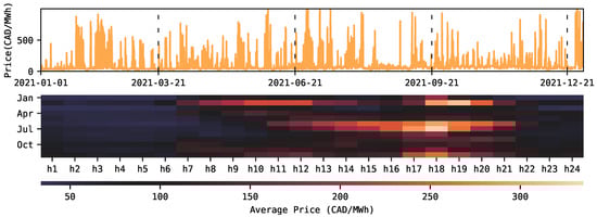
Figure 1. (Top): Alberta’s spot market prices for the year 2021. (Bottom): Monthly average of hourly Alberta’s spot prices at each hour of the day.

Figure 2 shows a comparison of the occurrence of price spikes between Alberta’s HAPP [27], Ontario’s Hourly Ontario Energy Price [28] (HOEP), and New York’s Locational-Based Marginal Price (LBMP) [29] in 2021. Prices are clustered based on different price thresholds in $/MWh (CAD/MWh for HAPP and HOEP, and USD/MWh for New York LBMP). Ontario’s electricity market [28] is also a single-settlement real-time wholesale power pool, while the New York market [29] is a two-settlement, day-ahead, and real-time market. For the latter, the real-time LBMP of a high-demand zone (i.e., Zone J or the one corresponding to New York City) is considered. Observe from Figure 2 that the occurrence of price spikes in Alberta’s market surpasses the other two markets at all the different thresholds. Furthermore, as the threshold increases towards $ 500/MWh, the occurrence of spikes for the Ontario and New York electricity markets dramatically decreases. For example, for the threshold between $ 400/MWh and $ 500/MWh, neither of these two markets registered any price spikes, while for that above $ 500/MWh, the occurrence of three price spikes for both the Ontario and New York markets was detected.

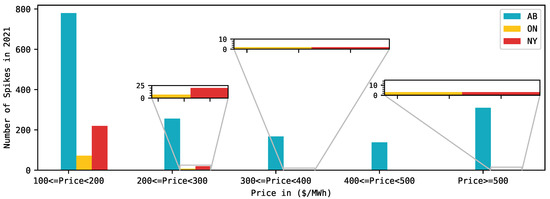
Figure 2. Comparison of the occurrence of the number of price spikes between the Alberta, Ontario, and New York (real-time) electricity markets using different price thresholds in $/MWh (CAD/MWh for HAPP and HOEP, and USD/MWh for New York LBMP). For the New York market, we show the New York City zone, i.e., the highest demand zone in the New York electricity market.

Electricity price spikes can occur for several hours and this occurrence depends upon the system’s available supply and electric demand [8], but also can depend on the bidding strategies used by different market participants [30]. Higher-cost operating generators become operative usually when the demand increases, and they normally influence the price causing the occurrence of price spikes [5]. The increasing number of price spikes in Alberta’s electricity market means that expensive operating generators (usually gas generators) have been required during the on-peak hours to meet demand. Furthermore, among other reasons, like higher demand and higher gas prices, for the year 2021, for example, the occurrence of price spikes is also associated with changes in the bidding strategies of large market participants [26], following the expiration of their long-term power purchase agreements (PPAs). In other words, those participants are no longer subject to the contractual terms established in their PPAs to recover their fixed and variable operation costs, but now, they are recovered directly from the energy market.

As previously discussed, higher volatility levels can be observed in real-time electricity markets [31]. Using the measure of return variation, ${\sigma }_{h,T}$, presented in [1], we conduct a comparative analysis of hourly spot price return variations between the Alberta, Ontario, and New York electricity markets. For the latter, again, we selected the load zone J (i.e., New York City zone), being the one having higher load concentration in that market. In this analysis, the time series of spot prices are scaled to zero–one. The return variations are calculated first, as the difference between the spot price at time, t, and the spot price at $t-h$. For example, in [1], intra-hour return variations are calculated, i.e., $h=1$. Second, each difference is divided by the average value of the spot prices over T, e.g., $T=3$ (2019, 2020, and 2021) years in our case. Finally, ${\sigma }_{h,T}$ can be estimated as the standard deviation of the price differences over T. Furthermore, due to the increasing levels of renewable penetration, zero or negative spot prices can frequently be observed in modern electricity markets [32]; hence, we decide to use ${\sigma }_{h,T}$, as defined in [1], to overcome the associated problems with arithmetic or logarithmic returns. In other words, prices differences, $r_{t,h}$, are defined as follows:

$$\begin{array}{c}\hfill r_{t,h}={\displaystyle \frac{p_t-p_{t-h}}{\frac{1}{T}{\sum }_{i=1}^T{p}_i}},\end{array}$$

(1)

where $p_t$ denotes the spot price at time, t; $p_{t-h}$ the spot price at $t-h$; and T is the overall number of prices ($T=3$ years in our case). Finally, the return variation, ${\sigma }_{h,T}$, can be calculated as follows:

$$\begin{array}{c}\hfill {\sigma }_{h,T}=\sqrt{{\displaystyle \frac{{\sum }_{t=1}^{N_o}{\left(r_{t,h}-{\overline{r}}_{h,T}\right)}^2}{N_o-1}}},\end{array}$$

(2)

where $N_o$ is the number of prices differences, $r_{t,h}$, and ${\overline{r}}_{h,T}$ is the simple $r_{t,h}$ average, all of them over the time window, T. Considering the volatility indices presented in [31], we extend the analysis for $h=\{1,24,168\}$, i.e., intra-hour, trans-day, and trans-week return variations, respectively.

Table 1 shows the results for the return variations ${\sigma }_{\{1,3\}}$, ${\sigma }_{\{24,3\}}$, and ${\sigma }_{\{168,3\}}$ for each electricity market. Higher values are shown in bold letters. From the results observed in Table 1, Alberta’s market presents the higher three-year return variations for each case, i.e., intra-day, trans-day, and trans-week. For example, Alberta’s intra-day return variations (i.e., ${\sigma }_{\{1,3\}}$) are, on average, 5.3 times higher than intra-day return variations from the other analyzed markets. Likewise, Alberta’s trans-day (i.e., ${\sigma }_{\{24,3\}}$) and trans-week (i.e., ${\sigma }_{\{168,3\}}$) return variations are, on average, 6.5 and 6.1 times higher than those from the other markets, respectively.

Table 1. Return variations for $T=3$ corresponding to the years 2019, 2020, and 2021 (unit-less numbers).

3-Year Period
	${\mathbf{\sigma }}_{\mathbf{1},\mathbf{3}}$	${\mathbf{\sigma }}_{\mathbf{24},\mathbf{3}}$	${\mathbf{\sigma }}_{\mathbf{168},\mathbf{3}}$
Alberta	0.92	1.74	2.11
Ontario	0.35	0.41	0.43
New York-RT	0.13	0.18	0.22
New York-DA	0.14	0.31	0.57

Furthermore, we observe from Table 1 that trans-week variations show the highest value in all markets. For example, on average, ${\sigma }_{\{168,3\}}$ is 2.3 times higher than ${\sigma }_{\{1,3\}}$ for all the analyzed electricity markets; similarly, ${\sigma }_{\{168,3\}}$ is 1.3 times higher than ${\sigma }_{\{24,3\}}$. As [31] found in their work, trans-week price fluctuations are wider than those observed intra-hourly. From the analyzed period T, and based on observations from Table 1, we can conclude that higher return variations tend to occur in single-settlement electricity markets like Alberta’s and Ontario’s. This is in comparison with two-settlement electricity markets, like the one in New York. Furthermore, Alberta’s market presents higher intra-hour, trans-day, and trans-week return variations, thus, showing the challenging market dynamic faced by the proposed electricity price forecasting model.

2.2. Long Short-Term Memory Networks

Deep learning techniques have recently gained strength in the field of electricity price forecasting, mainly associated with the available computational power, volumes of data, and complexities of modern electricity markets [20]. Recurrent neural networks (RNNs) are a popular method in time series forecasting. The structure of RNN consists of an input layer, one or more hidden layers, and an output layer. RNNs have a chain-like structure where connections between nodes form a directed graph along a temporal sequence. In contrast to feed-forward neural networks, RNNs include a feedback loop that allows the neural network to receive a sequence of inputs. In other words, in RNNs, the output of $t-1$ is fed back into the network, having an impact on the outcome of step t and for each subsequent step, allowing information to persist. For this reason, different types of RNNs, like long short-term memory (LSTM) or gated recurrent units (GRUs) have been used for electricity price forecasting [20,33]. In RNN, the backpropagation algorithm is used to calculate gradients and adjust weights between network layers during training [34]. Nevertheless, the weights update scheme could stop the neural network from further training. The reason is that after a long chain, the gradient could vanish or increase notoriously. In other words, RNNs face many difficulties in learning from a long-term dependency [35]. Long short-term memory neural networks are a variant of RNNs. They were proposed to address the drawbacks of the RNN on learning long-term dependencies [18] by including more interactions per module or cell and by remembering information for prolonged periods [36].

A typical LSTM network consists of memory blocks called cells. The cell state and the hidden state are transferred to the next cell. The main chain of data flow is given by the cell state, which permits the data to flow forward basically unchanged. Nevertheless, some linear transformations can happen and, via sigmoid gates, some data can be removed or added to the cell state. A gate is similar to a series of matrix operations that comprise distinct individual weights. Since the gates control the memorizing process, the LSTM networks can avoid the long-term dependency problem [36]. The operation of the LSTM network is illustrated in (3a)–(3f):

$$\begin{array}{cc}\hfill & f_t=sigmoid(W_f[h_{t-1},x_t]+b_f)\hfill \end{array}$$

(3a)

$$\begin{array}{cc}\hfill & i_t=sigmoid(W_i[h_{t-1},x_t]+b_i)\hfill \end{array}$$

(3b)

$$\begin{array}{cc}\hfill & o_t=sigmoid(W_o[h_{t-1},x_t]+b_o)\hfill \end{array}$$

(3c)

$$\begin{array}{cc}\hfill & g_t=tanh(W_g[h_{t-1},X_t]+b_g)\hfill \end{array}$$

(3d)

$$\begin{array}{cc}\hfill & c_t=f_t\odot c_{t-1}+i_t\odot g_t\hfill \end{array}$$

(3e)

$$\begin{array}{cc}\hfill & h_t=o_t\odot tanh\left(c_t\right)\hfill \end{array}$$

(3f)

where $f_t$ is the forget gate that by the sigmoid function decides which information is not required and is going to be omitted or forgotten from the cell. In (3b), $i_t$ is the input gate that determines the amount of information of the network input, $x_t$, but also the previous hidden state, $h_{t-1},$ that can pass into the memory cell. In (3c) and (3d), $g_t$ is the update gate that creates a vector of new cell values, and $o_t$ is the output gate that controls the amount of information of the current memory cell that can pass to the hidden state ($h_t$) in (3f). In (3e), $c_t$ is the cell state that updates itself recursively by the interaction of its old value ($c_{t-1}$) with forget and input gates’ values. In addition, $W_f$, $W_i$, $W_o$, and $W_g$ are the weights matrices of the forget gate, input gate, output gate, and update gate, respectively. The biases of the forget gate, input gate, output gate, and update gate are represented by $b_f$, $b_i$, $b_o$, and $b_g$.

Among others, electricity price forecasting is one of the research fields where LSTM neural networks have been used. By analyzing the market coupling impact on electricity price forecasts, different hybrid topologies of autoencoders based on LSTM and convolutional neural networks have been used to forecast the day-ahead electricity prices in the Nord Pool electricity market [37]. Similarly, considering European market integration, ref. [20] used different deep learning topologies, one consisting of a hybrid deep learning forecasting model based on an LSTM and a convolutional neural network, to generate day-ahead price forecasts for several European countries. In [15], different forecasting models consisting of a single LSTM neural network and an LSTM part of one hybrid and two ensemble forecasting models were used to forecast day-ahead prices for the German market at one-, seven-, and thirty-day-ahead forecasting horizons. Similarly, ref. [38] used a statistical spike filter [8,20,39], Wavelet decomposition on the spot prices time series, in combination with an Adam-optimized LSTM neural network, to forecast electricity prices for the New South Wales region in Australia and French electricity markets. In [33], shallow and deep architectures of LSTM neural networks were used to forecast day-ahead electricity prices for the Turkish electricity market.

2.3. Extreme Gradient Boosting

Extreme gradient boosting, also called XGBoost, is a scalable machine learning for tree boosting that was proposed by [19]. XGBoost is optimized under the gradient boosting framework. The concept of boosting is to combine a series of models with low accuracy (weak models) to build a more robust model with better prediction performance. Gradient boosting uses the residual of previous models to correct the next model. It is called gradient boosting because it uses the gradient descent algorithm to minimize the loss function when adding new models. As an improvement, XGBoost adds regularization to the loss function, having, in this way, a better performance against over-fitting.

Let us consider a data set, $S=\{(x_l,p_l):l=1,\cdots ,n,x_l\in {\mathbb{R}}^m,p_l\in \mathbb{R}\}$, where there are n samples with m features or variables. The predicted value of the model is defined as follows:

$$\begin{array}{c}\hfill {\widehat{p}}_l=\sum _{a=1}^K{f}_a\left(x_l\right),f_a\in F,\end{array}$$

(4)

where $x_l$ is the l-th training sample, $f_a$ represents an independent decision tree, $f_a\left(x_l\right)$ indicates the prediction score given by the a-th tree to the l-th sample, and F is the space of functions containing all the regression trees. XGBoost uses the same concept of gradient boosting but improves it by a adding regularization to the objective function to measure the model performance:

$$\begin{array}{c}\hfill J=\sum _{l=1}^{n}L\left(p_l,{\widehat{p}}_l\right)+\sum _{a=1}^K\mathsf{\Omega }\left(f_a\right).\end{array}$$

(5)

The L term represents a training loss function, which measures how well the model fits on training data. $\mathsf{\Omega }$ is the regularization term that avoids over-fitting by penalizing the complexity of the model (i.e., the regression tree functions), and is given by [19]:

$$\begin{array}{c}\hfill \mathsf{\Omega }\left(f_a\right)=\gamma T+{\displaystyle \frac{1}{2}}\lambda \sum _{s=1}^T{w_s}^2,\end{array}$$

(6)

where T is the number of leaves in a decision tree, $\lambda$ is a parameter to scale the penalty, $\gamma$ is the complexity of each leaf, and w is the vector of scores on leaves. The tree ensemble model is trained in an additive manner. Each time a new tree is added, the score is equal to the previous score plus the new tree’s score. Considering ${{\widehat{p}}_l}^{\left(b\right)}$, the prediction of the l-th sample at the b-th iteration, the objective function at the b-ith iteration is given by the following:

$$\begin{array}{c}\hfill J^{\left(b\right)}=\sum _{l=1}^{n}L\left(p_l,{\widehat{p}}_l^{\left(b-1\right)}+f_b\left(x_l\right)\right)+\mathsf{\Omega }\left(f_b\right).\end{array}$$

(7)

Then, the second-order Taylor expansion is used to optimize the objective in the general setting. Assuming the loss function, L, is the mean square error (MSE), the objective function can finally be estimated as follows:

$$\begin{array}{c}\hfill {\tilde{J}}^{\left(b\right)}=\sum _{l=1}^n\left[{\delta }_l{f}_b\left(x_l\right)+{\displaystyle \frac{1}{2}}{\theta }_l{f}_b{\left(x_l\right)}^2\right]+\mathsf{\Omega }\left(f_b\right),\end{array}$$

(8)

where ${\delta }_l={\partial }_{{\widehat{p}}_l^{\left(b-1\right)}}L\left(p_l,{\widehat{p}}_l^{\left(b-1\right)}\right)$ and ${\theta }_l={\partial }_{{\widehat{p}}_l^{\left(b-1\right)}}^{2}L\left(p_l,{\widehat{p}}_l^{\left(b-1\right)}\right)$ are the first and second gradient of the loss function, L. The objective function can finally be rewritten as:

$$\begin{array}{cc}\hfill & {\tilde{J}}^{\left(b\right)}=\sum _{l=1}^n\left[{\delta }_l{f}_b\left(x_l\right)+{\displaystyle \frac{1}{2}}{\theta }_l{f}_b{\left(x_l\right)}^2\right]+\gamma T+{\displaystyle \frac{1}{2}}\lambda \sum _{s=1}^T{w_s}^2,\hfill \end{array}$$

(9a)

$$\begin{array}{cc}\hfill & {\tilde{J}}^{\left(b\right)}=\sum _{s=1}^T\left[\left(\sum _{l\in I_s}{\delta }_l\right)w_s+{\displaystyle \frac{1}{2}}\left(\sum _{l\in I_s}{\theta }_l+\lambda \right){w_s}^2\right]+\gamma T,\hfill \end{array}$$

(9b)

where $I_s=\left\{l\right|q\left(x_l\right)=s\}$ denotes the instance set of a leaf, s. For a fixed tree structure, q, the optimal weight, $w_s^{*}$, of a leaf, s, and the corresponding optimal value can be obtained by:

$$\begin{array}{cc}\hfill & w_s^{*}=-{\displaystyle \frac{{\sum }_{l\in I_s}{\delta }_l}{{\sum }_{l\in I_s}{\theta }_l+\lambda }},\hfill \end{array}$$

(10a)

$$\begin{array}{cc}\hfill & {\tilde{J}}^{*}=-{\displaystyle \frac{1}{2}}\sum _{s=1}^T{\displaystyle \frac{{\left({\sum }_{l\in I_s}{\delta }_l\right)}^2}{{\sum }_{l\in I_s}{\theta }_l+\lambda }}+\gamma T.\hfill \end{array}$$

(10b)

Equation (10b) can be used as a scoring function to measure the quality of a tree structure, q. A smaller value $\tilde{J}$ means a better structure of the tree. Since it is impossible to enumerate all the possible tree structures, q, a greedy algorithm that starts from a single leaf and iteratively adds branches to the tree is used instead. $I_L$ and $I_R$ are the instance sets of the left and right nodes after the split, with $I=I_L\cup I_R$. The gain formula, which is often used for evaluating the split candidates, is obtained by enumerating the feasible segmentation points and selecting the maximum gain partition and the minimum target function:

$$\begin{array}{c}\hfill G={\displaystyle \frac{1}{2}}\left[{\displaystyle \frac{{\left({\sum }_{l\in I_L}{\delta }_l\right)}^2}{{\sum }_{l\in I_L}{\theta }_l+\lambda }}+{\displaystyle \frac{{\left({\sum }_{l\in I_R}{\delta }_l\right)}^2}{{\sum }_{l\in I_R}{\theta }_l+\lambda }}-{\displaystyle \frac{{\left({\sum }_{l\in I}{\delta }_l\right)}^2}{{\sum }_{l\in I}{\theta }_l+\lambda }}\right]-\gamma \end{array}$$

(11)

Among others, boosting tree-ensemble-based algorithms have been part of the modeling strategies of leader-board teams in important energy forecasting competitions, e.g., GEFCom2014 [40,41]. XGBoost is not the exception, and its robustness postulates it as a good candidate within the energy forecasting research field. For example, [42] used an ensemble model to generate one-hour-ahead locational marginal price forecasts for the New England day-ahead electricity market. The forecasting model is composed of two “relevance support vector machines” and an XGBoost regressor. Particularly, the latter is used to model the complex behavior of the price spikes. Additionally, [43] developed a hybrid forecasting model based on ANN with entity embedding to pre-process categorical data and an XGBoost regressor to forecast the day-ahead electricity prices in the PJM market.

2.4. Related Works

Hybrid electricity price forecasting systems consist of a combination of two or more existing price forecasting methods. These systems can be composed of only parametric, non-parametric, or a combination of both types of modeling approaches [15,44]. For example, in [45], a hybrid system consisting of committee machines was employed to recursively generate electricity price forecasts within a 4-hour-ahead forecasting horizon. Each of the two forecasting models is composed of two support vector machines and two multi-layer perceptron Levenberg–Marquardt ANNs. This hybrid system was tested using data from real-time and day-ahead electricity markets, i.e., the Alberta and West Denmark Zone (Nordic) electricity markets, respectively.

A hybrid system composed of a seasonal auto-regressive integrated moving average model and a deep belief network was used by [46] to forecast half-hourly and hourly electricity normal and spiky prices, respectively. The analyzed markets correspond to the Australian, Spanish, and PJM electricity markets. Similarly, ref. [8] proposed a hybrid forecasting model purely based on ANNs to forecast normal and spiky prices in the real-time electricity market of Ontario. Forecasts were generated for a 24-hour-ahead forecasting horizon. In [47], a hybrid mid-term electricity price forecasting system was proposed. Each of the three models consists of an auto-regressive integrated moving average model, along with principal component analysis, and an ANN model. The system is used to recursively generate forecasts of weekly average electricity prices for a 12-week forecasting horizon in the Brazilian electricity market.

Some previous studies have focused on building forecasting models for volatile, real-time markets [8]. For example, using data from the Ontario electricity market, ref. [9] forecasted 24-hour-ahead HOEP with ANN and fuzzy logic systems. Similarly, ref. [48] generated 3- and 24-hour-ahead electricity price forecasts using time series models and ANN in the Ontario market. In [49], half-hour-ahead forecasts for the Australian electricity market were generated using an extreme learning machine. Using daily electricity spot prices and a higher-order hidden Markov chain model in discrete time, the work in [50] generated one-step-ahead forecasts on a daily forecasting horizon for the Alberta electricity market. The model estimation was conducted through the decomposition of the time series of spot prices into a seasonal and stochastic component, like in [51,52]. The former was modeled as the combination of sinusoidal functions, and the latter as the combination of an Ornstein–Uhlenbeck process and an additive compound Poisson component.

Some of the existing works have focused specifically on modeling and forecasting price spikes in electricity markets. In [2], the demand-to-capacity ratio was used to estimate the probability of the occurrence of price spikes in the UK electricity market using a forecasting horizon that extends from 2 days up to 2 weeks ahead. The authors in [53] proposed an auto-regressive Poisson model to forecast one-day-ahead price spikes in different interconnected regions of the Australian electricity market. The model used three exogenous variables and the short-term history of price spike occurrence. In reference [54], the authors studied the mutual effects of interconnected regions within the Australian electricity market on the occurrence of price spikes. To do so, a dynamic copula-based multivariate discrete choice model generated one-step-ahead predictions of the probability of price spike occurrence using half-hourly historical prices of electricity. In a classification approach, reference [55] used a variable threshold, along with feature selection via the Fisher score, to classify price spikes using a support vector machine for the Australian electricity market. However, the horizon over which the classification of new spikes was made was not specified.

Our proposed method distinguishes itself from the existing approaches by employing a different approach to model combination in two dimensions. Conventional methods typically combine models in a “vertical” dimension, where multiple models are ensembled to generate forecasts for the same fixed forecast horizon. In contrast, our method combines models vertically, specifically focusing on enhancing the predictive ability of our model in detecting and predicting price spikes. Additionally, we combine models at a “horizontal” dimension to take advantage of available market data for each forecast horizon and generate forecasts for an extended 96-hour-ahead forecasting horizon. In other words, we break the forecast horizon into multiple segments and train and build a model for each segment, depending on what explanatory features are available at each horizontal dimension. Furthermore, in the existing works that have used Alberta’s market prices for their base case, no particular emphasis has been made on enhancing the ability of the models to predict the price spikes.

3. Methodology

Let us denote the hourly market price at time, t, with $p_t$. Furthermore, we refer to the feature space as $\mathbf{X}=\{{\mathbf{x}}_j,j=1,\cdots ,N\}$, where ${\mathbf{x}}_j$ is the $j^{th}$ feature. The proposed method is composed of five horizontally cascaded forecasting models, i.e., $E_i,\{i=1,\cdots ,5\}$. Each model uses a subset of $\mathbf{X}$, referred to here as ${\mathrm{\Phi }}_i$. Furthermore, each ${\mathrm{\Phi }}_i$ contains a set of observed and predicted inputs that are selected depending on their availability and usefulness. $E_i$s are only different in their corresponding set of features and the associated forecasting horizons. More specifically, $E_1$ to $E_5$ are used to generate 1-hour-ahead, 2- to 3-hour-ahead, 4-hour-ahead, 5- to 24-hour-ahead, and 25- to 96-hour-ahead price forecasts, respectively. Let us refer to the final $k_i$-step-ahead price forecasts generated by model $E_i$ using the feature set, ${\mathrm{\Phi }}_i$, as $\left\{{\widehat{p}}_{t+k_i}\right|{\mathrm{\Phi }}_i\}$; thus, $k_i$ can be specified as $k_1=1$, $k_2\in \{2,3\}$, $k_3=4$, $k_4\in \{5,\cdots ,24\}$, and $k_5\in \{25,\cdots ,96\}$. This horizontal cascading of the five models is shown in Figure 3. Observe from Figure 3 that a set of 96 price forecasts are generated at each time step, i.e., hourly, at the forecasting origin, t.

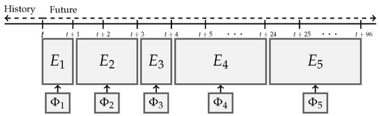
Figure 3. The horizontal dimension of the forecasting system. The width of each model represents how many forecasts are generated at each forecasting horizon. Moreover, each $E_i$ uses a different input set of features, ${\mathrm{\Phi }}_i$.

Each model, $E_i$, is composed of two predictors, i.e., an LSTM and an XGBoost. The predictors are “vertically” stacked up and independently produce what we call preliminary price forecasts for each of the associated forecasting horizons. The final price forecasts, i.e., ${\widehat{p}}_{t+k_i}$, are defined accordingly as follows:

$$\begin{array}{c}\hfill {\widehat{p}}_{t+k_i}=\left\{\begin{array}{c}{\tilde{p}}_{t+k_i}^{\left(XGB\right)}\mathrm{if}{\tilde{p}}_{t+k_i}^{\left(LSTM\right)}<T_1\hfill \\ {\tilde{p}}_{t+k_i}^{\left(LSTM\right)}\mathrm{if}{T}_1\le {\tilde{p}}_{t+k_i}^{\left(LSTM\right)}<T_2\hfill \\ {\tilde{p}}_{t+k_i}^{\left(XGB\right)}\mathrm{if}{\tilde{p}}_{t+k_i}^{\left(LSTM\right)}\ge T_2\hfill \end{array}\right.\end{array}$$

(12)

In (12), we refer to the preliminary forecasts produced by the two predictors for the k step ahead as ${\tilde{p}}_{t+k_i}^{\left(LSTM\right)}$ and ${\tilde{p}}_{t+k_i}^{\left(XGB\right)}$. The preliminary price forecasts generated by the LSTM models are compared against two price spike thresholds, $T_1$ and $T_2$, where $T_1<T_2$. Essentially, the final forecasts are picked from either the LSTM model or the XGBoost models, depending on if they are normal, i.e., ${\tilde{p}}_{t+k_i}^{\left(LSTM\right)}<T_1$; a spike, i.e., $T_1\le {\tilde{p}}_{t+k_i}^{\left(LSTM\right)}<T_2$; or a super-spike, i.e., ${\tilde{p}}_{t+k_i}^{\left(LSTM\right)}\ge T_2$. The observation is that the LSTM model performed better in predicting the trends and the sequences of prices, as expected. However, the XGBoost models outperformed the LSTM models for both low and very high prices. In this paper, finding the exact values of the two thresholds is conducted by examining the models’ performance on the training data sets with some trial and error. However, determining the thresholds and even the weight of combining the two forecasts could be automated and optimized, which is left for future work. Figure 4 presents how the LSTM models and XGBoost models are integrated in this methodology and how they contribute to obtain the final price forecasts, ${\widehat{p}}_{t+k_i}$, for each $E_i$ model along each forecasting horizon, $k_i$ (i.e., the horizontal dimension). Here, a different input set, ${\varphi }_i$, is used (i.e., the vertical dimension) depending on $k_i$.

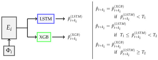
Figure 4. Integration of XGBoost and LSTM models in the proposed methodology to obtain final price forecasts, ${\widehat{p}}_{t+k_i}$, for each $E_i$ model that deploys a different input set of features, ${\mathrm{\Phi }}_i$.

A key factor to enhance the performance of the proposed model is to identify as many publicly input features that are available for a given forecast horizon. Here, we describe the features that we identified for Alberta’s market. Electricity price time series show significant autocorrelation, and the literature is accordingly rich on how to choose the most informative lags using tools such as autocorrelation functions [48,56]. We define the subset feature, ${\mathbf{x}}_1=p_{t-l}$, to include the autocorrelated lagged values of the prices [56,57] up to 168 previous hours. The AESO [27] publishes hourly load forecasts [9,11,58], wind energy production forecasts [11], and the total generation availability forecasts [20] for each technology for up to seven days ahead; we refer to these features as ${\mathbf{x}}_2$, ${\mathbf{x}}_3$, and ${\mathbf{x}}_4$, respectively. On the other hand, the AESO publishes the forecast imports/exports of energy into and from Alberta for the next 48 h. This feature is referred to here by ${\mathbf{x}}_5$. Although they do not use forecasts of the imports/exports, some works have used historical values of this variable (for example, [37,59,60]).

We propose to employ a new feature for price forecasting in this paper. Thermal generators often play a key role in electricity markets where they make up a significant portion of the supply side. This is the case, for example, in Alberta where coal and gas units make up 75% [26] of the total installed capacity (end of 2021). A sudden change in the output of the thermal units could indicate a change in the market supply curve and could help predict sharp changes in the prices in the short term. Thus, we propose to use the slope of the output of the online thermal generation capacity as a new feature, and we refer to it as ${\mathbf{x}}_6$. The slope is defined as the change in the output power over the past 10 min period. Moreover, the AESO also publishes pool price forecasts [61] for the next three hours. We, hence, define this feature subset as ${\mathbf{x}}_7$. Additionally, the latest system marginal price (SMP) values are found to be a useful input [61] in price forecasting models. The modeler may choose to feed its model with one or more of the latest available SMP values before the model is run. This feature is referred to as ${\mathbf{x}}_8$ here.

Based on the availability of the identified features, the following feature subsets, ${\mathrm{\Phi }}_i$, are proposed:

$$\begin{array}{cc}\hfill & {\mathrm{\Phi }}_1=\left\{{\mathbf{x}}_1,{\mathbf{x}}_2,{\mathbf{x}}_3,{\mathbf{x}}_4,{\mathbf{x}}_5,{\mathbf{x}}_6,{\mathbf{x}}_7,{\mathbf{x}}_8\right\}\hfill \end{array}$$

(13a)

$$\begin{array}{cc}\hfill & {\mathrm{\Phi }}_2=\left\{{\mathbf{x}}_1,{\mathbf{x}}_2,{\mathbf{x}}_3,{\mathbf{x}}_4,{\mathbf{x}}_5,{\mathbf{x}}_6,{\mathbf{x}}_7\right\}\hfill \end{array}$$

(13b)

$$\begin{array}{cc}\hfill & {\mathrm{\Phi }}_3=\{{\mathbf{x}}_1,{\mathbf{x}}_2,{\mathbf{x}}_3,{\mathbf{x}}_4,{\mathbf{x}}_5,{\mathbf{x}}_6\}\hfill \end{array}$$

(13c)

$$\begin{array}{cc}\hfill & {\mathrm{\Phi }}_4=\{{\mathbf{x}}_1,{\mathbf{x}}_2,{\mathbf{x}}_3,{\mathbf{x}}_4,{\mathbf{x}}_5\}\hfill \end{array}$$

(13d)

$$\begin{array}{cc}\hfill & {\mathrm{\Phi }}_5=\{{\mathbf{x}}_1,{\mathbf{x}}_2,{\mathbf{x}}_3,{\mathbf{x}}_4\}\hfill \end{array}$$

(13e)

In (13a)–(13b), ${\mathrm{\Phi }}_i$ corresponds to a multiple input to each $E_i$, and depending on the forecasting horizon, the output of $E_i$ is single (i.e., $k=1,4$-hour-ahead) or multiple (i.e., k = 2–3-, 5–24-, or 25–96-hour-ahead) point forecast(s). $E_1$ takes advantage of all the information that we have, including the latest SMPs, the slope of the thermal generation, and the AESO price forecasts. On the other hand, we discovered that including the latest SMP does not improve model accuracy; thus, ${\mathbf{x}}_8$ is excluded from $E_2$. AESO price forecasts are not available for a 4-hour-ahead forecasting horizon; thus, the model for this horizon does not include ${\mathbf{x}}_7$. However, it is often observed in Alberta that price spikes last longer than one hour; thus, the slope of thermal generators, i.e., ${\mathbf{x}}_6$ is included in the input set for $E_3$. When it comes to import/export forecasts, their accuracy often drops for the second day. Thus, their forecasts are only considered for the next 24 h. This is the main reason for creating model $E_4$, to focus on 5 to 24 hours ahead, where ${\mathbf{x}}_5$ is included in the input set of this model. The last model, i.e., $E_5$, benefits from the least available information, simply because not all of the identified features are available or useful for a long horizon for up to 96 h.

4. Numerical Results

In this section, we present the numerical results of the proposed hybrid forecasting system. Furthermore, we show the convenience of using the slope of the online thermal generators’ output power as a feature, i.e., ${\mathbf{x}}_6$. Alberta’s electricity market dataset comprises three years of data, ranging from January 2017 to December 2019. The training set considers data from January 2017 to July 2018; likewise, a validation set considers data from August 2018 to December 2018. The rest of the data, i.e., January 2019 to December 2019, is used for testing. In general, we use two years of data for training and validation, and one year for testing [11]. Moreover, $k_i$-step-ahead hourly price forecasts are generated following a forward rolling window. This is a common practice in electricity price forecasting [11,62]. However, in our case, the computational burden makes it challenging for the model to be recalibrated daily; thus, monthly recalibration results in a better choice.

The input data from where the LSTM [18] and XGBoost [19] models are estimated is scaled between $[-1,1]$[20]. The inverse of this transformation is applied to the price forecasts at the error calculation stage [20]. Furthermore, hyperparameter tuning for each $E_i$ is conducted via grid search and evaluated on the validation set [11]. Likewise, due to its simple implementation, computational efficiency, and small memory requirements, the Adam algorithm [63] is selected to optimize the LSTM models. The corresponding hyperparameter search spaces for the LSTM and XGBoost models are presented in Table 2 and Table 3, respectively.

Table 2. Hyperparameter search space for the LSTM models.

Hyperparameter	Values
Neurons in 1st LSTM layer	4, 8, 16, 32, 64, 96, 128
Neurons in 2nd LSTM layer	4, 8, 16, 32, 64, 96, 128
Activation function of 1st layer	Sigmoid, tanh, relu, linear
Activation function of 2nd layer	Sigmoid, tanh, relu, linear
Dimension of 1st dense layer	7, 14, 21, 28, 35

Table 3. Hyperparameter search space for the XGBoost models.

Hyper-Parameter	Values
Regularization ($\lambda$)	0.3, 0.5, 0.7
Minimum split loss $\gamma$	0.3, 0.5, 0.7
Tree depth	6, 8, 10
Learning rate ($\eta$)	0.1, 0.3, 0.5
Loss	Root-mean-square error

The grid search algorithm systematically explores all possible combinations of hyperparameter values from Table 2 and Table 3. For each combination of hyperparameters, the model is trained on the training set, and its performance is evaluated using the mean squared error as the chosen metric on the validation set. The hyperparameter combination that yields the best result, based on the chosen evaluation metric, is selected. Finally, once the best hyperparameters are identified, the model is retrained using the training dataset, incorporating the optimized hyperparameter values.

The forecasting accuracy evaluation is conducted using two performance metrics, i.e., the root-mean-square error (RMSE) and the mean absolute error (MAE). Both can be expressed as follows:

$$\begin{array}{cc}\hfill & \mathrm{MAE}={\displaystyle \frac{1}{N_h}}\sum _{e=1}^{N_h}\left|p_{m_e}-{\widehat{p}}_{m_e}\right|\hfill \end{array}$$

(14a)

$$\begin{array}{cc}\hfill & \mathrm{RMSE}=\sqrt{{\displaystyle \frac{1}{N_h}}\sum _{e=1}^{N_h}{\left(p_{m_e}-{\widehat{p}}_{m_e}\right)}^2}\hfill \end{array}$$

(14b)

In (14a) and (14b), $m\in \{1,2,3,\cdots ,96\}$, $N_h$ is the number of hours in the evaluation period, i.e., the test period. Likewise, $p_{m_e}$ and ${\widehat{p}}_{m_e}$ are the actual and predicted pool prices, respectively. Finally, the fixed price thresholds [5,53] presented in (12) correspond to $T_1\ge CAD150$/MWh and $T_2\ge CAD400$/MWh.

4.1. Electricity Price Forecasting with the Proposed Model

The proposed multi-horizon price forecasting system generates forecasts using a different set of regressors, $E_i$ (i.e., the vertical dimension), throughout the forecasting horizons (i.e., the horizontal dimension) $k_1=1$, $k_2\in \{2,3\}$, $k_3=4$, $k_4\in \{5,\cdots ,24\}$, and $k_5\in \{25,\cdots ,96\}$. Furthermore, each $E_i$ uses a different input set, ${\mathrm{\Phi }}_i$, depending on the market data availability at the forecasting origin (see Section 3).

Figure 5 displays a comparison of the RMSE and MAE between the proposed forecasting system and a set of benchmark models. These benchmark models consist of a decision tree regressor (DTR), an LSTM, and an XGBoost. All models have the same inputs and training periods. Observe that the proposed hybrid forecasting system consistently outperforms the benchmark models along all the forecasting horizons, i.e., $k_1=1$ hour ahead, $k_2\in \{2,3\}$ hours ahead, $k_3=4$ hours ahead, $k_4\in \{5,\cdots ,24\}$ hours ahead, and $k_5\in \{25,\cdots ,96\}$ hours ahead. As expected, shorter forecasting horizons present the lowest error rates. Observe, for example, the RMSE and MAE for $k_1=1$ hour ahead, $k_2\in \{2,3\}$ hours ahead, and $k_3=4$ hours ahead are somewhere around CAD 38-65/MWh and CAD 10-24/MWh, respectively. The reason is because these forecasts contain the most recent market information (i.e., close to real time) from ${\mathbf{x}}_6$, ${\mathbf{x}}_7$, and ${\mathbf{x}}_8$ (see Section 3).

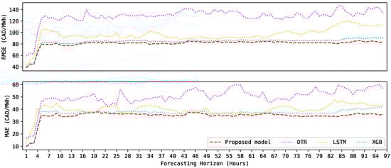
Figure 5. Performance comparison between the proposed model (dashed line) and a set of benchmark models (dotted lines) for the testing period. (Top): root-mean-square error (RMSE). (Bottom): mean absolute error (MAE).

Beyond $k_3=4$ hours ahead, i.e., from $k_4\in \{5,\cdots ,24\}$ hours ahead up to $k_5\in \{25,\cdots ,96\}$ hours ahead, both the RMSE and MAE increase by approximately CAD 15/MWh and CAD 10/MWh, respectively. Observe that once they reach somewhere around CAD 80/MWh (RMSE) and CAD 35/MWh (MAE), both error metrics are kept almost constant. This demonstrates the capabilities of the proposed hybrid forecasting system to forecast long sequences of data without considerably decreasing its performance, i.e., significantly increasing the error.

Likewise, we demonstrate the usefulness of deploying different forecasting regressors following the proposed methodology. To do so, we compare the proposed hybrid forecasting system against a single LSTM forecaster, i.e., a single regressor that generates pool price predictions ${\widehat{p}}_{t+k_{\{1-96\}}}^{\left(LSTM\right)}$. Observe that these predictions are made for all the forecasting horizons, from $k_1=1$ hour ahead up to $k_{96}=96$ hours ahead. The single forecaster is trained, validated, and tested using all input variables. Figure 6 shows the 96-hour-ahead forecasts made by the proposed forecasting system and the single forecaster for an arbitrary test period. Observe that the proposed model could effectively predict more price spikes (i.e., $p_t>T_1$) than the single forecaster model. For example, the group of spikes between August 14 and 15 in Figure 6 is better captured by the proposed multi-horizon forecasting system than from the single forecaster. Similarly, this can be observed on 16 August 2019.

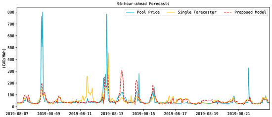
Figure 6. Forecast comparison between the proposed model and a single forecaster for the 96-hour-ahead forecasting horizon between 8 August 2019 and 22 August 2019.

Based on the results shown in Figure 6, we estimate and compare the average RMSE and MAE along all $k_i$s for the proposed forecasting model and a single forecaster. The average RMSE for the proposed forecasting model is CAD 66.41/MWh, compared to CAD 70.81/MWh for the single forecaster. Likewise, the average MAE for the proposed forecasting model is CAD 20.06/MWh, compared to CAD 21.78/MWh for the single forecaster. Overall, the proposed hybrid cascading forecasting model enhances the accuracy of the price spike predictions.

4.2. Impact of the Slope of Power Production of Thermal Generators on the Performance of the Developed Forecasting System

The slope of power production of thermal generators during the initial minutes of the first predicted hour is a novel feature (i.e., ${\mathbf{x}}_{\mathbf{6}}$) of the proposed forecasting system. For example, coal generators usually offer blocks of power at low prices; thus, a reduction in output power could be indicative of price spikes in Alberta’s electricity market. Furthermore, thermal generators (e.g., coal generators) have a steady ramp-up and ramp-down curve; therefore, their power production slope can help to determine if they are going to be available for the next two or three hours.

Figure 7 (left) shows an example case where three price spikes occurred in Alberta’s market on 8 August 2019. Each price spike is shown with a value of CAD 762.83/MWh, CAD 507.4/MWh, and CAD 801.68/MWh. Furthermore, their occurrence is within the on-peak hours window, i.e., between 2:00 p.m. and 5:00 p.m. The main cause of these price spikes is associated with a reduction in thermal generation availability. Observe in Figure 7 (left) how the thermal units Thermal Gen 1 and Thermal Gen 2 reduced their power production considerably after midday. Thermal Gen 1 goes completely offline at 2:15 p.m., and Thermal Gen 2 reduces its production around 2:00 p.m., 3:00 p.m., and, again, at 4:00 p.m. during that day.

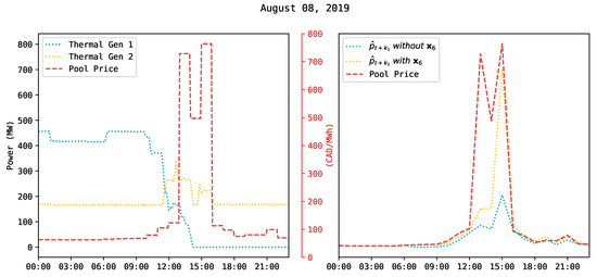
Figure 7. The arbitrarily selected period of 8 August 2019. (Left): Pool price dynamic reaction to changes in thermal generation. (Right): One-hour-ahead forecast (i.e., ${\widehat{p}}_{t_{k+1}}$) with and without using ${\mathbf{x}}_{\mathbf{6}}$ as a feature.

For the same period shown in Figure 7 (left), the dispatched energy of the economic merit order table from the AESO [27] indicates that high-price power blocks of other thermal generation units set high spot prices during these hours. To demonstrate the contribution that the slope of power production of thermal generators (i.e., ${\mathbf{x}}_{\mathbf{6}}$) has on the model’s capabilities to better predict price spikes, Figure 7 (right) compares the one-hour-ahead forecasts (i.e., ${\widehat{p}}_{t+1}$) produced by $E_1$ for the same period on 8 August 2019. As an example, we present the RMSE and MAE for this specific period. When using ${\mathbf{x}}_{\mathbf{6}}$, the RMSE and MAE are CAD 140.63/MWh and CAD 46.74/MWh, respectively. Likewise, if ${\mathbf{x}}_{\mathbf{6}}$ is not used, the RMSE and MAE are CAD 197.79/MWh and CAD 75.09/MWh, respectively. This example shows the impact of ${\mathbf{x}}_{\mathbf{6}}$ on the proposed model’s performance. In other words, using ${\mathbf{x}}_{\mathbf{6}}$ enhances the model’s ability to forecast price spikes.

4.3. Price Spike Predictions Accuracy Assessment

As previously emphasized, the proposed forecasting model is designed to enhance the prediction of price spikes. Thus, we analyze its performance to detect price spikes for the one-hour-ahead and four-hour-ahead forecasting horizons. The selection of these forecasting horizons is because, in Alberta’s market, different market participants benefit from these forecasts (see Section 1). For example, large load consumers benefit from the one-hour-ahead forecasts to decide if they need to reduce their demand. Likewise, generators benefit from the four-hour-ahead price forecasts to decide if they need to modify their bidding strategies. To conduct the analysis, we use the spike prediction confidence (SPC) and spike prediction accuracy (SPA) metrics [60]:

$$\begin{array}{c}\hfill \mathrm{SPC}(\%)={\displaystyle \frac{N_{corr}}{N_{as}}}\end{array}$$

(15)

$$\begin{array}{c}\hfill \mathrm{SPA}(\%)={\displaystyle \frac{N_{corr}}{N_{sp}}}\end{array}$$

(16)

In (15) and (16), $N_{corr}$ corresponds to the number of correctly predicted price spikes. Similarly, $N_{as}$ is the total number of predicted price spikes, and $N_{sp}$ is the actual number of price spikes. Moreover, prices greater than or equal to CAD 150/MWh (see definition of $T_1$ in Section 4) are used to decide whether a price is considered a spike, normal, or otherwise. The SPA and SPC metrics are computed for each month [61] in the test period, i.e., the year 2019. In each case, the final spike detection performance of the models is assessed with the average over this period. The higher the values of both SPA and SPC, the better the performance of the model.

Table 4 shows the results for the SPC corresponding to the one-hour-ahead forecasts. Observe that the proposed model has the highest SPC compared to the benchmark models. In other words, the proposed model outperforms the benchmark models in not labeling normal prices as price spikes. Similarly, Table 5 shows the performance of the proposed model and the benchmark models on the SPA metric for the one-hour-ahead forecasts. Here, the proposed model has the highest SPA compared to the benchmark models. Consequently, the proposed model is better at detecting price spikes compared to the benchmark models.

Table 4. SPCs (%) for one-hour-ahead price forecasts for the different models.

Month	Proposed Model	DTR	LSTM	XGB
January	100	12.5	66.7	12.5
February	87.5	44.7	72	44.7
March	87.1	61.5	84.4	70.5
April	77.8	41.1	80	56.2
May	91.7	67.1	88.2	71.4
June	83.3	75	83.3	69.7
July	69.2	54.5	75	33.3
August	70.5	40	68.8	57.1
September	83.3	64.2	89.4	44.1
October	72.7	19.3	58.3	22.2
November	72.7	65.5	82.6	43.7
December	68.7	44.4	66.7	28.6
Average	80.4	49.1	76.3	46.2

Table 5. SPAs (%) for one-hour-ahead price forecasts for the different models.

Month	Proposed Model	DTR	LSTM	XGB
January	25	25	50	25
February	65.3	62.6	72	62.7
March	71.1	63.1	71	63.2
April	58.3	58.3	66.7	75
May	78.6	87.5	80.4	80.4
June	75.8	63.6	75.8	69.7
July	64.3	42.8	64.3	57.1
August	75	50	68.8	75
September	87	78.2	73.9	65.2
October	66.7	50	58.3	33.3
November	80	63.3	63.3	46.7
December	91.7	66.6	66.7	66.7
Average	69.9	59.3	67.6	60

Likewise, Table 6 and Table 7 show the four-hour-ahead SPC and SPA of the proposed model and the benchmark models. As expected, the performance of all the models in terms of the four-hour-ahead SPC and SPA is lower than the performance shown for the one-hour-ahead. The reason for this is that as we move forward to further forecasting horizons, the spike detection capability of the models tends to decrease. Moreover, we can observe from Table 6 and Table 7 that the proposed model has again the highest SPC and SPA when compared to the benchmark models. For the SPC, the proposed model is better than the benchmark models in not labeling normal prices as price spikes. Similarly, for the SPA, the proposed model is better at detecting price spikes. Observe that for both of the analyzed forecasting horizons, the proposed model demonstrates a superior balance between SPC and SPA when compared to the benchmarks.

Table 6. SPCs (%) for four-hour-ahead price forecasts for the different models.

Month	Proposed Model	DTR	LSTM	XGB
January	23	5.8	0	5.8
February	35.7	32.2	61.7	32.2
March	43.5	28.5	22.2	6.4
April	85.7	16.7	50	26.6
May	67.1	44.1	60	32.7
June	73.3	4.0	60	24
July	42.8	53.8	14.3	12.5
August	42.8	37.5	29.6	24
September	71.4	35.7	66.7	15.6
October	29.7	12.5	36.8	11.5
November	45	30.7	58.5	18.8
December	15.3	0	13.3	9.5
Average	47.9	25.1	39.4	18.3

Table 7. SPAs (%) for four-hour-ahead price forecasts for the different models.

Month	Proposed Model	DTR	LSTM	XGB
January	75	25	0	25
February	86.7	49.3	38.7	49.3
March	44.7	15.7	5.2	7.8
April	50	33.3	8.3	33.3
May	83.9	60.7	80.4	33.9
June	66.7	3.0	27.3	18.18
July	42.8	100	7.1	7.14
August	37.5	37.5	50	37.5
September	65.2	43.4	34.8	30.4
October	91.7	16.7	58.3	25
November	76.7	80	76.7	50
December	16.7	0	16.7	33.3
Average	61.5	38.7	33.6	29.2

Finally, observe that the differences between the proposed model and the XGBoost are relatively small in terms of the RMSE and MAE ( see Figure 5). However, when evaluating their performance based on the SPC and SPA metrics (Table 4, Table 5, Table 6 and Table 7), it is evident that the proposed model outperforms the XGBoost. Thus, when enhancing the capabilities of a forecasting model to predict price spikes, it is important to evaluate not only the accuracy of the point predictions but the spike detection ability of the model.

5. Evaluation of the Economic Value of the Developed Price Forecasting Model in Alberta

In this section, we evaluate the economic advantage of the proposed price forecasting model in the ancillary services market, in particular, to the spinning reserve offers of one generation facility. Moreover, an optimization problem is proposed to maximize the revenues from the contingency reserve volume offers based on the electricity price forecasts, ${\widehat{p}}_{t+k_i}$, of each $E_i$.

For the generation facility, the optimization considers the maximum power (MW) to distribute active and standby operating reserves across the daily on-peak and off-peak periods. Likewise, the prices of each offer are not changed in the optimization problem and are assumed to be low enough to be dispatched first on their respective merit order tables. In other words, the generation facility is assumed to be a price-taker, so its operation in the market does not affect the prices. Unlike the two optimized models, which both consider maximum power for the offers in the spinning reserves market, we consider the other three approaches, i.e., the first, second, and third approach. The first approach considers 10 MW and 5 MW of the volume offers for the active and standby spinning market, respectively. Similarly, the second (third) approach uses 12 MW (8 MW) and 3 MW (7 MW). The offers for the second and third approaches also correspond to the active and standby spinning market.

The total actual revenues from January to December 2019 are calculated using daily volume offers and the actual electricity prices from both the energy and ancillary services markets. The total possible revenues are obtained using the actual electricity price to solve the optimization problem, i.e., the perfect approach. Similarly, we solve, again, the optimization problem using price forecasts, ${\widehat{p}}_{t+k_i}$, instead of the actual electricity price to calculate the revenues in this scenario. We call this approach the proposed model.

The difference between the perfect approach and the proposed model revenues represents the effect of the price forecast inaccuracies in the proposed forecasting system. Likewise, the total actual revenues are also compared against the other three approaches that do not consider any optimization techniques on their volume offers, i.e., the first, second, and third approaches.

Table 8 presents the total obtained revenues from each approach at the spinning reserves market. Observe that the proposed model provides the highest revenues when compared with the first, second, and third approaches. Its total revenues represent 89.67% of the maximum revenues that could have been obtained from the perfect approach. The difference in revenues between the developed model and the perfect approach is approximately CAD $450,000$ per year. This difference represents the economic losses brought by the forecast inaccuracies, e.g., approximately equivalent to 10% per year of the maximum possible revenues. We recognize these inaccuracies are related to the ideas presented in Section 1 on the challenges of producing single-digit price forecast errors in real-time electricity markets.

Table 8. Total revenues from the spinning reserve volume offers between January and December 2019, i.e., the test period.

Methodology	Revenue (Million CAD)
Perfect approach	4.35
Proposed model	3.90
First approach	2.70
Second approach	2.98
Third approach	2.43

Observe also from Table 8 that the proposed model outperforms, on average, by more than 30 % or approximately CAD $1,197,000$ per year compared to the revenues obtained from fixed volume offers, i.e., first, second, and third approaches. Table 8 also shows that for the case of the fixed volume offers, it is more profitable to increase the offers in the active spinning reserve market and decrease those in the standby spinning reserve market. Observe, for example, the difference in revenues of approximately more than CAD $500,000$ per year between the second and third approaches.

Finally, Figure 8 shows the combined cumulative revenues for both types of spinning reserves (i.e., active and standby) for the analyzed period in 2019. It is possible to observe that the revenues between the perfect approach and the developed model significantly differ from the other three approaches approximately after February 2019. Likewise, observe the impact of the forecast error between the perfect approach and the developed model after March 2019. Such a tendency prevails and increases towards the end of the analyzed period.

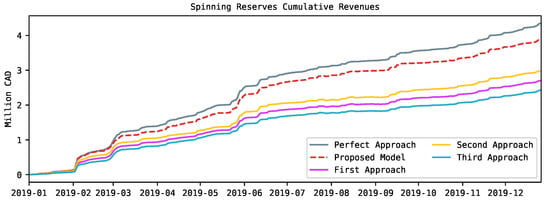
Figure 8. Total cumulative revenues from the spinning reserve volume offers in the test period. These results correspond to the economic evaluation of the proposed forecasting system compared to other approaches.

6. Conclusions

A hybrid electricity price forecasting model that takes advantage of a two-dimension strategy was presented in this paper. At the vertical dimension, the different forecasting regressors generated price predictions based on a stack array of an XGBoost and an LSTM model. Likewise, at the horizontal dimension, the proposed model took advantage of the available market information at the forecasting origin to generate price forecasts from 1 h ahead up to 96 h ahead. In addition, the novel input feature based on the slope of the output power production of thermal generators demonstrated and improvement in the price spike prediction accuracy of the proposed forecasting model.

Extensive numerical results were conducted to evaluate the accuracy of the proposed point forecasting model, and also to evaluate its ability to detect the occurrence of price spikes in the Alberta electricity market for the year 2019. In terms of MAE and RMSE, the proposed forecasting model outperformed the other benchmark models along all the forecasting horizons. The MAE and RMSE errors for price predictions from one to four hours ahead range between CAD 10–24/MWh and CAD 38–65/MWh, respectively. From five to ninety-six hours ahead, the MAE and RMSE increased by approximately CAD 10/MWh and CAD 15/MWh, respectively. Both error metrics also kept almost constant during this forecasting horizon, which demonstrates the capabilities of the proposed hybrid forecasting system to forecast long sequences of data without considerably decreasing its performance. Furthermore, our experiments showed that the proposed forecasting model enhanced the prediction of price spikes at further forecasting horizons when compared to a single forecaster. Moreover, in terms of the price spike detection assessment, we showed that the proposed forecasting model outperformed, on average, the benchmark models for both the SPC and SPA metrics. This demonstrates the importance of conducting a specific spike detection evaluation of the models to assure their performance not only in predicting, but also in detecting the occurrence of price spikes at different forecasting horizons.

Finally, the proposed price forecasting model was effectively employed to allocate, in the most profitable way possible, the contingency reserve volume offers of a hypothetical generation facility in the ancillary services market in Alberta. The output of the optimization problem showed that the proposed forecasting model was able to provide higher revenues for the generation facility when compared to the other presented approaches. Moreover, we also demonstrated that the impact of the forecast error in our study case represents a loss in revenues of approximately 10% per year of what could have been if a perfect approach was used.

One limitation of this study is that the proposed price forecasting model does not directly consider the historical offers and bids submitted by market players. By not considering these crucial inputs, the model may overlook important market dynamics and potential strategic behaviors, which could impact the accuracy of its forecasts. Incorporating the offers and bids of market players into the model has the potential to enhance its performance by capturing the influence of participant strategies and optimizing the forecasting outcomes. However, it is important to note that such types of input data are not publicly available in all markets. Future research should explore the integration of these additional inputs to further refine and strengthen the predictive capabilities of the model. Several other limitations should also be noted:

• The input of recent variations in the output power of thermal units as an indicator of unplanned outages or shifts in the supply stack may be more relevant to coal generators, as their ramp-up and ramp-down times are typically longer compared to gas generators. The proposed methodology was tested using data from Alberta’s electricity market, where more than five coal generators were still operational (the year 2019).
• The literature presents some benchmark models for comparison for day-ahead market price forecasts [11]. However, it lacks a standard benchmark model for testing price forecasting methods for real-time markets focused on price spike detection. Thus, we have reported the results of comparing the proposed method with two baseline models that we have developed to evaluate the performance of the proposed method.
• The price spike thresholds ($T_1$ and $T_2$) will vary among different electricity markets and depend on the frequency and magnitude of price spikes. The optimal selection of these thresholds should be based on the training dataset specific to the electricity market under study. Automating and optimizing the process of determining these thresholds is recommended for future research.
• The proposed methodology was only tested on the Alberta electricity market, which features the presence of more than five coal generators (the year 2019). However, it can be applied to other electricity markets where the presence of large generation units can have an impact on prices.

Furthermore, it is essential to acknowledge the significance of quantifying uncertainties associated with deterministic forecasts. As part of future research, developing a probabilistic forecasting model based on the proposed strategy would be valuable in addressing this aspect.

References

- Mayer, K.; Trück, S. Electricity Markets around the World. J. Commod. Mark. 2018, 9, 77–100. [Google Scholar] [CrossRef]
- Maryniak, P.; Weron, R. What is the Probability of an Electricity Price Spike? Evidence from the UK Power Market. In Handbook of Energy Finance: Theories, Practices Furthermore, Simulations; Goutte, S., Nguyen, D., Eds.; World Scientific: Hackensack, NJ, USA, 2019; pp. 231–245. [Google Scholar]
- Ciarreta, A.; Martinez, B.; Nasirov, S. Forecasting electricity prices using bid data. Int. J. Forecast. 2022, 39, 1253–1271. [Google Scholar] [CrossRef]
- Weron, R. Electricity price forecasting: A review of the state-of-the-art with a look into the future. Int. J. Forecast. 2014, 30, 1030–1081. [Google Scholar] [CrossRef]
- Christensen, T.; Hurn, A.; Lindsay, K. Forecasting spikes in electricity prices. Int. J. Forecast. 2012, 28, 400–411. [Google Scholar] [CrossRef]
- Haben, S.; Caudron, J.; Verma, J. Probabilistic Day-Ahead Wholesale Price Forecast: A Case Study in Great Britain. Forecasting 2021, 3, 596–632. [Google Scholar] [CrossRef]
- Tschora, L.; Pierre, E.; Plantevit, M.; Robardet, C. Electricity price forecasting on the day-ahead market using machine learning. Appl. Energy 2022, 313, 118752. [Google Scholar] [CrossRef]
- Sandhu, H.; Fang, L.; Guan, L. Forecasting day-ahead price spikes for the Ontario electricity market. Electr. Power Syst. Res. 2016, 141, 450–459. [Google Scholar] [CrossRef]
- Rodriguez, C.; Anders, G. Energy Price Forecasting in the Ontario Competitive Power System Market. IEEE Trans. Power Syst. 2004, 19, 366–374. [Google Scholar] [CrossRef]
- Aggarwal, S.K.; Saini, L.M.; Kumar, A. Electricity Price Forecasting in Ontario Electricity Market Using Wavelet Transform in Artificial Neural Network Based Model. Int. J. Control Autom. Syst. 2008, 6, 639–650. [Google Scholar]
- Lago, J.; Marcjasz, G.; De Schutter, B.; Weron, R. Forecasting day-ahead electricity prices: A review of state-of-the-art algorithms, best practices and an open-access benchmark. Appl. Energy 2021, 293, 116983. [Google Scholar] [CrossRef]
- Gomez, T.; Herrero, I.; Rodilla, P.; Escobar, R.; Lanza, S.; de la Fuente, I.; Llorens, M.L.; Junco, P. European Union Electricity Markets: Current Practice and Future View. IEEE Power Energy Mag. 2019, 17, 20–31. [Google Scholar] [CrossRef]
- Aggarwal, S.K.; Saini, L.M.; Kumar, A. Electricity Price Forecasting in Deregulated Markets: A Review and Evaluation. Int. J. Electr. Power Energy Syst. 2009, 31, 13–22. [Google Scholar] [CrossRef]
- Sgarlato, R.; Ziel, F. The Role of Weather Predictions in Electricity Price Forecasting Beyond the Day-Ahead Horizon. IEEE Trans. Power Syst. 2022, 38, 2500–2511. [Google Scholar] [CrossRef]
- Lehna, M.; Scheller, F.; Herwartz, H. Forecasting Day-Ahead Electricity Prices: A Comparison of Time Series and Neural Network Models Taking External Regressors into Account. Energy Econ. 2022, 106, 105742. [Google Scholar] [CrossRef]
- Complete Set of ISO Rules. Available online: https://www.aeso.ca/rules-standards-and-tariff/iso-rules/complete-set-of-iso-rules/ (accessed on 7 July 2020).
- Liu, L.; Bai, F.; Su, C.; Ma, C.; Yan, R.; Li, H.; Sun, Q.; Wennersten, R. Forecasting the occurrence of extreme electricity prices using a multivariate logistic regression model. Energy 2022, 247, 123417. [Google Scholar] [CrossRef]
- Hochreiter, S.; Schmidhuber, J. Long Short-Term Memory. Neural Comput. 1997, 9, 1735–1780. [Google Scholar] [CrossRef]
- Chen, T.; Guestrin, C. XGBoost: A Scalable Tree Boosting System. In Proceedings of the 22nd ACM SIGKDD International Conference On Knowledge Discovery and Data Mining, San Francisco, CA, USA, 13–17 August 2016; pp. 785–794. [Google Scholar]
- Lago, J.; De Ridder, F.; De Schutter, B. Forecasting spot electricity prices: Deep learning approaches and empirical comparison of traditional algorithms. Appl. Energy 2018, 221, 386–405. [Google Scholar] [CrossRef]
- International Institute of Forecasters. Available online: https://forecasters.org/foresight/beyond-error-measures/ (accessed on 18 July 2022).
- Wu, H.; Levinson, D. The ensemble approach to forecasting: A review and synthesis. Transp. Res. Part Emerg. Technol. 2021, 132, 103357. [Google Scholar] [CrossRef]
- AESO. Electricity in Alberta. Available online: https://www.aeso.ca/aeso/electricity-in-alberta/ (accessed on 23 March 2020).
- AESO. Understanding the Market. Available online: https://www.aeso.ca/market/understanding-the-market/ (accessed on 24 March 2020).
- AESO. Guide to Understanding Alberta’s Electricity Market. Available online: https://www.aeso.ca/aeso/understanding-electricity-in-alberta/continuing-education/guide-to-understanding-albertas-electricity-market/ (accessed on 23 March 2020).
- AESO. 2021 Annual Market Statistics. Available online: https://www.aeso.ca/market/market-and-system-reporting/annual-market-statistic-reports/ (accessed on 28 September 2022).
- AESO. Available online: http://www.aeso.ca (accessed on 19 August 2022).
- IESO. Available online: http://www.ieso.ca (accessed on 28 July 2022).
- NYISO. Available online: http://www.nyiso.com (accessed on 28 July 2022).
- Weron, R. Modeling and Forecasting Electricity Loads and Prices: A Statistical Approach; John Wiley & Sons: Chichester, UK; Hoboken, NJ, USA, 2006; pp. 25–64. [Google Scholar]
- Zareipour, H.; Bhattacharya, K.; Cañizares, C.A. Electricity market price volatility: The case of Ontario. Energy Policy 2007, 35, 4739–4748. [Google Scholar] [CrossRef]
- Uniejewski, B.; Weron, R.; Ziel, F. Variance Stabilizing Transformations for Electricity Spot Price Forecasting. IEEE Trans. Power Syst. 2018, 33, 2219–2229. [Google Scholar] [CrossRef]
- Ugurlu, U.; Oksuz, I.; Tas, O. Electricity Price Forecasting Using Recurrent Neural Networks. Energies 2018, 11, 1255. [Google Scholar] [CrossRef]
- Jiang, L.; Hu, G. Day-Ahead Price Forecasting for Electricity Market using Long-Short Term Memory Recurrent Neural Network. In Proceedings of the 2018 15th International Conference on Control, Automation, Robotics and Vision (ICARCV), Singapore, 18–21 November 2018; pp. 949–954. [Google Scholar] [CrossRef]
- Bengio, Y.; Simard, P.; Frasconi, P. Learning long-term dependencies with gradient descent is difficult. IEEE Trans. Neural Netw. 1994, 5, 157–166. [Google Scholar] [CrossRef] [PubMed]
- Le, X.H.; Ho, H.V.; Lee, G.; Jung, S. Application of Long Short-Term Memory (LSTM) Neural Network for Flood Forecasting. Water 2019, 11, 1387. [Google Scholar] [CrossRef]
- Li, W.; Becker, D.M. Day-Ahead Electricity Price Prediction Applying Hybrid Models of LSTM-based Deep Learning Methods and Feature Selection Algorithms under Consideration of Market Coupling. Energy 2021, 237, 121543. [Google Scholar] [CrossRef]
- Chang, Z.; Zhang, Y.; Chen, W. Electricity Price Prediction Based on Hybrid Model of Adam Optimized LSTM Neural Network and Wavelet Transform. Energy 2019, 187, 115804. [Google Scholar] [CrossRef]
- Lu, X.; Dong, Z.Y.; Li, X. Electricity market price spike forecast with data mining techniques. Electr. Power Syst. Res. 2005, 73, 19–29. [Google Scholar] [CrossRef]
- Gaillard, P.; Goude, Y.; Nedellec, R. Additive Models and Robust Aggregation for GEFCom2014 Probabilistic Electric Load and Electricity Price Forecasting. Int. J. Forecast. 2016, 32, 1038–1050. [Google Scholar] [CrossRef]
- Hong, T.; Pinson, P.; Fan, S.; Zareipour, H.; Troccoli, A.; Hyndman, R.J. Probabilistic Energy Forecasting: Global Energy Forecasting Competition 2014 and Beyond. Int. J. Forecast. 2016, 32, 896–913. [Google Scholar] [CrossRef]
- Agrawal, R.K.; Muchahary, F.; Tripathi, M.M. Ensemble of Relevance Vector Machines and Boosted Trees for Electricity Price Forecasting. Appl. Energy 2019, 250, 540–548. [Google Scholar] [CrossRef]
- Xie, H.; Chen, S.; Lai, C.; Ma, G.; Huang, W. Forecasting the Clearing Price in the Day-Ahead Spot Market Using eXtreme Gradient Boosting. Electr. Eng. 2022, 104, 1607–1621. [Google Scholar] [CrossRef]
- Weron, R.; Bierbrauer, M.; Trück, S. Modeling electricity prices: Jump diffusion and regime switching. Phys. Stat. Mech. Its Appl. 2004, 336, 39–48. [Google Scholar] [CrossRef]
- Motamedi, A.; Geidel, C.; Zareipour, H.; Rosehart, W.D. Electricity price forecasting considering residual demand. In Proceedings of the 2012 3rd IEEE PES Innovative Smart Grid Technologies Europe (ISGT Europe), Berlin, Germany, 14–17 October 2012; pp. 1–8. [Google Scholar] [CrossRef]
- Zhang, J.; Tan, Z.; Wei, Y. An Adaptive Hybrid Model for Short Term Electricity Price Forecasting. Appl. Energy 2020, 258, 114087. [Google Scholar] [CrossRef]
- Filho, J.C.R.; Affonso, C.d.M.; De Oliveira, R.C. Energy Price Prediction Multi-Step Ahead Using Hybrid Model in the Brazilian Market. Electr. Power Syst. Res. 2014, 117, 115–122. [Google Scholar] [CrossRef]
- Zareipour, H.; Canizares, C.; Bhattacharya, K.; Thomson, J. Application of Public-Domain Market Information to Forecast Ontario’s Wholesale Electricity Prices. IEEE Trans. Power Syst. 2006, 21, 1707–1717. [Google Scholar] [CrossRef]
- Chen, X.; Dong, Z.Y.; Meng, K.; Xu, Y.; Wong, K.P.; Ngan, H.W. Electricity Price Forecasting With Extreme Learning Machine and Bootstrapping. IEEE Trans. Power Syst. 2012, 27, 2055–2062. [Google Scholar] [CrossRef]
- Xiong, H.; Mamon, R. A higher-order Markov chain-modulated model for electricity spot-price dynamics. newblock Appl. Energy 2019, 233–234, 495–515. [Google Scholar] [CrossRef]
- Janczura, J.; Trück, S.; Weron, R.; Wolff, R.C. Identifying Spikes and Seasonal Components in Electricity Spot Price Data: A Guide to Robust Modeling. Energy Econ. 2013, 38, 96–110. [Google Scholar] [CrossRef]
- Afanasyev, D.O.; Fedorova, E.A. On the Impact of Outlier Filtering on the Electricity Price Forecasting Accuracy. Appl. Energy 2019, 236, 196–210. [Google Scholar] [CrossRef]
- Christensen, T.; Hurn, S.; Lindsay, K. It Never Rains but It Pours: Modeling the Persistence of Spikes in Electricity Prices. Energy J. 2009, 30. [Google Scholar] [CrossRef]
- Manner, H.; Türk, D.; Eichler, M. Modeling and Forecasting Multivariate Electricity Price Spikes. Energy Econ. 2016, 60, 255–265. [Google Scholar] [CrossRef]
- Vu, D.H.; Muttaqi, K.M.; Agalgaonkar, A.P.; Bouzerdoum, A. A Multi-Feature Based Approach Incorporating Variable Thresholds for Detecting Price Spikes in the National Electricity Market of Australia. IEEE Access 2021, 9, 13960–13969. [Google Scholar] [CrossRef]
- Contreras, J.; Espinola, R.; Nogales, F.; Conejo, A.J. ARIMA models to predict next-day electricity prices. IEEE Trans. Power Syst. 2003, 18, 1014–1020. [Google Scholar] [CrossRef]
- Conejo, A.J.; Contreras, J.; Espínola, R.; Plazas, M.A. Forecasting Electricity Prices for a Day-Ahead Pool-Based Electric Energy Market. Int. J. Forecast. 2005, 21, 435–462. [Google Scholar] [CrossRef]
- Marcjasz, G.; Uniejewski, B.; Weron, R. Probabilistic Electricity Price Forecasting with NARX Networks: Combine Point or Probabilistic Forecasts? Int. J. Forecast. 2020, 36, 466–479. [Google Scholar] [CrossRef]
- Van Der Heijden, T.; Lago, J.; Palensky, P.; Abraham, E. Electricity Price Forecasting in European Day Ahead Markets: A Greedy Consideration of Market Integration. IEEE Access 2021, 9, 119954–119966. [Google Scholar] [CrossRef]
- Zhao, J.H.; Dong, Z.Y.; Li, X.; Wong, K.P. A Framework for Electricity Price Spike Analysis With Advanced Data Mining Methods. IEEE Trans. Power Syst. 2007, 22, 376–385. [Google Scholar] [CrossRef]
- Chitsaz, H.; Zamani-Dehkordi, P.; Zareipour, H.; Parikh, P.P. Electricity Price Forecasting for Operational Scheduling of Behind-the-Meter Storage Systems. IEEE Trans. Smart Grid 2018, 9, 6612–6622. [Google Scholar] [CrossRef]
- Marcjasz, G.; Uniejewski, B.; Weron, R. On the Importance of the Long-Term Seasonal Component in Day-Ahead Electricity Price Forecasting with NARX Neural Networks. Int. J. Forecast. 2019, 35, 1520–1532. [Google Scholar] [CrossRef]
- Kingma, D.P.; Ba, J. Adam: A Method for Stochastic Optimization. In Proceedings of the 3rd International Conference on Learning Representations, San Diego, CA, USA, 7–9 May 2015. [Google Scholar] [CrossRef]
Disclaimer/Publisher’s Note: The statements, opinions and data contained in all publications are solely those of the individual author(s) and contributor(s) and not of MDPI and/or the editor(s). MDPI and/or the editor(s) disclaim responsibility for any injury to people or property resulting from any ideas, methods, instructions or products referred to in the content. |
© 2023 by the authors. Licensee MDPI, Basel, Switzerland. This article is an open access article distributed under the terms and conditions of the Creative Commons Attribution (CC BY) license (https://creativecommons.org/licenses/by/4.0/).