Shrinking the Variance in Experts’ “Classical” Weights Used in Expert Judgment Aggregation

Abstract

Mathematical aggregation of probabilistic expert judgments often involves weighted linear combinations of experts’ elicited probability distributions of uncertain quantities. Experts’ weights are commonly derived from calibration experiments based on the experts’ performance scores, where performance is evaluated in terms of the calibration and the informativeness of the elicited distributions. This is referred to as Cooke’s method, or the classical model (CM), for aggregating probabilistic expert judgments. The performance scores are derived from experiments, so they are uncertain and, therefore, can be represented by random variables. As a consequence, the experts’ weights are also random variables. We focus on addressing the underlying uncertainty when calculating experts’ weights to be used in a mathematical aggregation of expert elicited distributions. This paper investigates the potential of applying an empirical Bayes development of the James–Stein shrinkage estimation technique on the CM’s weights to derive shrinkage weights with reduced mean squared errors. We analyze 51 professional CM expert elicitation studies. We investigate the differences between the classical and the (new) shrinkage CM weights and the benefits of using the new weights. In theory, the outcome of a probabilistic model using the shrinkage weights should be better than that obtained when using the classical weights because shrinkage estimation techniques reduce the mean squared errors of estimators in general. In particular, the empirical Bayes shrinkage method used here reduces the assigned weights for those experts with larger variances in the corresponding sampling distributions of weights in the experiment. We measure improvement of the aggregated judgments in a cross-validation setting using two studies that can afford such an approach. Contrary to expectations, the results are inconclusive. However, in practice, we can use the proposed shrinkage weights to increase the reliability of derived weights when only small-sized experiments are available. We demonstrate the latter on 49 post-2006 professional CM expert elicitation studies.

1. Introduction

When decisions are made under uncertainty, relying on the judgment of a single expert may not be advisable in practice. Hence, an expert group is usually used in formal expert elicitations, e.g., [1]. However, often only one single distribution, representing the combined expert judgments and uncertainty around them, is needed. This is known as an aggregation. There are two main approaches to aggregation: mathematical and behavioral.

In mathematical aggregation, separate judgments are elicited from the experts and probability distributions are fitted to each expert’s judgments. Then, separately fitted probability distributions are combined to form the aggregate distribution using a mathematical formula (a pooling rule). The behavioral approach requires the group of experts to discuss their judgments and to produce group “consensus” judgments to which a distribution will be fitted [1]. Here, we focus on the mathematical aggregation technique, where separately fitted experts’ probability distributions are combined using an appropriate mathematical formula. Two mathematical aggregation techniques are commonly used to obtain the aggregated distribution of an unknown quantity, namely the Bayesian approach and the opinion pooling approach [2]. In this paper, we discuss and aim to improve the latter.

Opinion pooling can be carried out to obtain an aggregated distribution of an unknown quantity by allocating equal weights to the experts’ probability distributions (for more details on opinion pooling, see Section 2.1). However, Cooke [2] showed that the levels of calibration and informativeness of experts’ elicited distributions can be different in practice. Therefore, applying equal weights for experts’ elicited distributions may not be appropriate. Cooke’s method [2], also referred to as the classical model (CM), proposes performance-based weights that incorporate both the calibration and the informativeness of experts’ elicited distributions.

Note that experts’ weights can randomly vary depending on experimental conditions, e.g., the nature and number of seed questions and time limitations. The seed questions that are used to derive weights are selected so that they are as similar as possible to the uncertain quantities of interest. Suppose we repeat the experiment under similar experimental conditions with the same number of new seed questions from the same background. The derived experts’ weights will most likely be different. Therefore, from a statistical point of view, it is important to consider experts’ weights as random variables and address the randomness of the derived weights when computing aggregated distributions of quantities. Even though performance-based CM weights often outperform equal weights in practice, they still fail to address the randomness of the derived weights when computing aggregated distributions of quantities. Addressing the above-mentioned randomness is the focus of this paper.

If experts’ weights are modeled as random variables, then estimating their mean becomes essential. Hence, we can now formulate the problem as a multivariate mean-estimation problem. Stein [3] showed that shrinkage estimation techniques can be used to obtain estimators of the mean of a multivariate normal distribution with reduced mean squared errors. Here, the interest is not to obtain an unbiased estimator, but an estimator with a reduced mean squared error. The James–Stein shrinkage estimator discussed in James and Stein [4] was proved to dominate the ordinary least squares estimator with a lower mean squared error in this context.

We propose using an empirical Bayes development of the James–Stein shrinkage estimation technique discussed in Zhao [5] that shrinks variables differently depending on their variances (larger variances correspond to more shrinkage). We apply this shrinkage to the CM weights to derive new weights that will enjoy reduced mean squared errors. The shrinkage estimation technique is not restricted to the estimation of mean of a multivariate normal distribution. Since 1956, a large body of research has focused on the application of the shrinkage estimation technique to obtain improved estimators of parameters for several statistical models (see [6] and references within). We nevertheless focus on its application to the estimation of the mean of a multivariate normal distribution.

2. Materials and Methods

2.1. CM Weights

Suppose n experts have provided their subjective probability distributions of an unknown quantity X. Let $f_e$ indicate the elicited distribution of X by the eth expert, where $e=1,2,\dots ,n$. Opinion pooling uses a simple linear combination of distributions elicited from n experts, say $f_1\left(x\right),f_2\left(x\right),\dots ,f_n\left(x\right)$, to obtain the aggregated distribution $f\left(x\right)$ of an unknown quantity X. Hence, $f\left(x\right)={\sum }_{e=1}^n{w}_e{f}_e\left(x\right)$. Note that $w_e$ is the weight allocated to the eth expert elicited distribution $f_e\left(x\right)$, for $e=1,2,3,\dots ,n$, and the sum of weights ${\sum }_{e=1}^n{w}_e=1$. Suppose equal weights are allocated to all the experts’ elicited distributions. Then, $w_e=\frac{1}{n}$ for all e and $f\left(x\right)$ will be the simple average of $f_e\left(x\right)$, for $e=1,2,3,\dots ,n$.

The CM proposes performance-based weights instead [2]. When using the CM, experts make separate judgments about the uncertain quantities of interest together with a number of seed (sometimes called calibration) questions whose true values are known to the analysts but are not immediately available to the experts during the elicitation. An expert’s performance (as measured by calibration and informativeness measures) on the seed questions is used as an indication of the expert’s expected performance on the uncertain quantities of interest. The seed questions are, therefore, selected so that they are as indicative as possible about expert performance with regard to the uncertain quantities of interest. Experts’ weights are then derived proportionally to these performance measures. The weighted experts’ distributions are then pooled. Deriving performance-based weights in this manner is the main feature of the CM. Cooke et al. [7] and Cooke and Goossens [8] have analyzed data sets elicited and combined using the CM and showed that, most often, CM-weighted pooling performs better than equal-weighted pooling.

The weights of the CM are proportional to the product of the calibration $\left(Cal\right)$ and informativeness $\left(Inf\right)$ [2]. Moreover, a threshold $\alpha$ can be used to filter out very poor calibration scores. For $\alpha >0$, let $1_{\alpha }\left(c\right)=1$ if $c\ge \alpha$, and 0 otherwise. Then, for all $\alpha >0$, the performance-based weight for expert e can be given as

$$w_{\alpha }\left(e\right)=Cal\left(e\right)\ast 1_{\alpha }\left(Cal\left(e\right)\right)\ast Inf\left(e\right).$$

The weight $w_{\alpha }\left(e\right)$ measures how concentrated (through $Inf\left(e\right)$) and how calibrated (through $Cal\left(e\right)$) expert e’s distributions are, while also making sure that the expert’s calibration is within an acceptable margin. It emphasizes the fact that eliciting concentrated distributions alone is not useful if they are not adequately calibrated. Hence, weights are assigned only to experts whose calibration scores exceed the threshold value $\alpha$ [9].

Details about the CM and the exact formulae for the calibration and informativeness scores can be found in Cooke [2], Quigley et al. [10] and Hanea and Nane [11]. It suffices to say here that the CM calibration is measured as the p-value or probability with which one would falsely reject the hypothesis that an expert’s probability judgments were calibrated, amounting to a hypothesis test. A near-zero calibration means that it is very unlikely for the discrepancy between an expert’s probability judgments and observed outcomes to be driven by chance.

Note that the p-value of the test statistic of the hypothesis test on the calibration above is a constant value and it is computed based on the assumption that the test statistic follows a chi-square distribution that depends on the number of seed questions (under the null hypothesis). The indicator function $1_{\alpha }\left(Cal\left(e\right)\right)$ is also a constant, namely 1 or 0 based on a comparison between two constant values $\alpha$ and $Cal\left(e\right)$. Moreover, the informativeness is also a constant. Therefore, overall, the computed experts’ weights are considered as fixed values in the CM.

2.2. Shrinkage Estimation of Weights

The concept behind considering experts’ weights as being random variables leads to a claim that the estimated experts’ weights from an experiment are realized values from the corresponding random variables. If the experiment was repeated under similar conditions, then other realized weights could be observed. Estimating the unknown population mean of experts’ weights using the observed set of experts’ weights (in given experiments) is a natural follow-up consideration. Thus, if we consider $w_1,w_2,\dots ,w_n$ as the estimated weights for n experts and ${\theta }_1,{\theta }_2,\dots ,{\theta }_n$ as the unknown population mean weights of experts, then we need to estimate the vector of population mean weights, $\theta =\{{\theta }_1,{\theta }_2,\dots ,{\theta }_n\}$, using a single realization of experts’ weights, $w=\{w_1,w_2,\dots ,w_n\}$, in a given experiment. According to Stein [3], this represents a small sample situation of which, in terms of mean squared error, the usual ordinary least squares estimates of mean parameters are not optimal and the James–Stein shrinkage estimator [4] can dominate the ordinary least squares estimator with a lower mean squared error in practice. We next review the James–Stein shrinkage estimation technique as presented in James and Stein [4]. This will provide the necessary background for applying the empirical Bayes development of the James–Stein shrinkage estimation technique proposed by Zhao [5]. It is this development that we propose using in order to derive shrinkage CM weights.

Suppose X is an $n–$variate normally distributed random variable with a vector $\theta$ of unknown means and a known covariance matrix ${\sigma }^{2}I$. Here, I is the $(n\times n)$ identity matrix and ${\sigma }^2$ is the assumed constant variance for all n variables of X. It follows that $X\sim N(\theta ,{\sigma }^{2}I)$. Consider the scenario of using a single $n–$variate observation of X to obtain an estimate $\widehat{\theta }$ of $\theta$ in this context. Hence, ${\widehat{\theta }}_{LS}=X$ is the ordinary least squares (OLS) estimator of $\theta$ in this situation considering the observations as estimates of $\theta$ themselves. This estimator is suboptimal in terms of mean squared error. It led to the development of the following James–Stein (JS) shrinkage estimator for $\theta$ by shrinking the OLS estimator towards the mean. The JS estimator $\left({\widehat{\theta }}_{JS}\right)$ for known ${\sigma }^2$ is given by

$${\widehat{\theta }}_{J{S}_1}=\left(1-\frac{(n-2){\sigma }^2}{{\Vert X\Vert }^2}\right)X,$$

(1)

and it dominates ${\widehat{\theta }}_{LS}$ in terms of lower mean squared error for any $n\ge 3$. If ${\sigma }^2$ is unknown and an estimator $S_l$ of ${\sigma }^2$, independent of X and distributed as ${\sigma }^2{\chi }_l^2$, is available (where l is the degrees of freedom of the ${\chi }^2$ distribution), then the JS estimator of $\theta$ is given by

$${\widehat{\theta }}_{J{S}_2}=\left(1-\frac{(n-2)S_l}{(l+2){\Vert X\Vert }^2}\right)X.$$

(2)

In the most realistic situation, $X\sim N(\theta ,\Sigma )$, $\Sigma$ being unknown. Suppose there is an independent estimator S of $\Sigma$, which is distributed as $W_{l-1}(s,\Sigma )$, where W is the Wishart distribution and $(l-1)$ indicates its corresponding degrees of freedom. James and Stein have proposed the following JS estimator in this situation as

$${\widehat{\theta }}_{J{S}_3}=\left(1-\frac{(n-2)}{(l-n+3)X^T{S}^{-1}X}\right)X.$$

(3)

It is worth noting that the the shrinkage estimators from Equations (1)–(3) are obtained by multiplying the original observations by a constant value. Thus, if we apply this technique on a set of derived experts’ weights, then the resulting shrinkage weights will be proportional to the originally derived weights. Hence, normalized CM weights before and after shrinkage will be identical. Instead, we could employ a shrinkage procedure that shrinks weights differently depending on a suitable factor. It seems practically useful to shrink weights differently depending on their variances, acknowledging the different levels of weights’ uncertainty through the shrinkage process. To do that, we propose using the empirical Bayes approach of obtaining shrinkage estimators of multivariate means discussed in Efron and Morris [12].

Suppose $w_e|{\theta }_e\sim N({\theta }_e,{\sigma }_e^2)$ are independent for $e=1,2,3,\dots ,n$, where ${\sigma }_e^2$ are known but different from one another. Furthermore, assume that ${\theta }_e\sim N(0,{\sigma }_{\theta }^2)$ are independent for $e=1,2,3,\dots ,n$ with an unknown constant variance ${\sigma }_{\theta }^2$. It follows that

$${\theta }_e|w_e\sim N((1-B_e)w_e,(1-B_e){\sigma }_e^2);e=1,2,3,\dots ,n,$$

where $B_e={\sigma }_e^2/({\sigma }_{\theta }^2+{\sigma }_e^2)$. Here, the empirical Bayes shrinkage estimator of ${\theta }_e$ is the posterior mean $E\left({\theta }_e\right|w_e)=(1-B_e)w_e$, with the Bayes risk $V\left({\theta }_e\right|w_e)=(1-B_e){\sigma }_e^2$ being less than the risk ${\sigma }_e^2$ of the least square estimator ${\widehat{\theta }}_e=w_e$. The shrinkage factor $1-B_e={\sigma }_{\theta }^2/({\sigma }_{\theta }^2+{\sigma }_e^2)$ here avoids the above-discussed problem of shrinking towards the origin by the same factor (the larger the value of ${\sigma }_e^2$, the larger the shrinkage). Even though this model produces different shrinkage factors for different variables $w_e$, the variances ${\sigma }_e^2$ are unknown in practice. Furthermore, assuming a specific value (zero) for the mean of the distribution of ${\theta }_e$ may not be applicable in general. Therefore, it would be practically more useful to find a general Bayes approach that deals with unknown means and variances of both the distributions of variables and the distributions of ${\theta }_e$ and $e=1,2,3,\dots ,n$ in the analysis.

Zhao [5] discussed an empirical Bayes approach of obtaining shrinkage estimators of multivariate means with unknown and unequal variances for n variables. The proposed double-shrinkage estimator shrinks both means and variances. According to Zhao [5], extensive numerical studies indicate that the double shrinkage estimator has lower Bayes risk than (i) the shrinkage estimator of means alone and (ii) the naive estimator with no shrinkage at all. In this approach, each variable $w_e$ is assumed to follow a normal distribution with mean ${\theta }_e$ and unknown variance ${\sigma }_e^2$, which differ across all the variables, and each ${\theta }_e$, with $e=1,2,3,\dots ,n$, is assumed to follow a common prior distribution $N(\mu ,{\tau }^2)$ with unknown mean $\mu$ and variance ${\tau }^2$. Therefore, the assumptions of this model appear to be more general than the assumptions of the model in Efron and Morris [12].

Suppose we derive the posterior distribution of ${\theta }_e$ using the model $w_e|{\theta }_e$, with ${\sigma }_e^2\sim N({\theta }_e,{\sigma }_e^2)$ and ${\theta }_e\sim N(\mu ,{\tau }^2)$ for $e=1,2,3,\dots ,n$, and assuming all the parameters of the model are known. Then, the posterior distribution of ${\theta }_e$ will be derived as

$${\theta }_e|w_e,{\sigma }_e^2\sim N(M_e{w}_e+(1-M_e)\mu ,M_e{\sigma }_e^2),$$

where $M_e={\tau }^2/({\tau }^2+{\sigma }_e^2)$. Therefore, for the known ${\sigma }_e^2$ case, the estimator for ${\theta }_e$ is $M_e{w}_e+(1-M_e)\mu ,$ which is the posterior expectation of ${\theta }_e$ given $w_e$ and ${\sigma }_e^2$. This estimator shrinks $w_e$ towards mean $\mu$ and the shrinkage factor $M_e={\tau }^2/({\tau }^2+{\sigma }_e^2)$ depends on the variance ${\sigma }_e^2$ of $w_e$. However, ${\sigma }_e^2,\mu$ and ${\tau }^2$ are assumed unknown in this context. Therefore, Zhao [5] derived the following double shrinkage estimator for $\theta$ in the form of

$${\widehat{\theta }}_e=\widehat{M_e}{w}_e+(1-\widehat{M_e})\widehat{\mu };$$

(4)

where $\widehat{M_e}={\widehat{\tau }}^2/({\widehat{\tau }}^2+{\widehat{\sigma }}_e^2)$, for $e=1,2,3,\dots ,n$, and $\widehat{\mu }={\sum }_{e=1}^n\frac{w_e/{\widehat{\sigma }}_e^2}{{\sum }_{e=1}^{n}1/{\widehat{\sigma }}_e^2}$. Observe that two estimators

$${\widehat{\tau }}^2={\left(\frac{{\sum }_{e=1}^n{(w_e-\widehat{\mu })}^2-S_e^2\exp (-m_e-{\sigma }_{ch,e}^2/2)}{n}\right)}_{+}$$

and

$${\widehat{\sigma }}_e^2=\exp \left({\widehat{M}}_{v,e}(\log \left(S_e^2\right)-m_e)+(1-{\widehat{M}}_{v,e}){\widehat{\mu }}_v\right)$$

are used to derive double shrinkage estimator of ${\theta }_e$ for $e=1,2,3\dots ,n$ in Equation (4) above. This empirical Bayes shrinkage estimator shrinks $w_e$, for $e=1,2,3,\dots ,n$ towards the weighted average $\widehat{\mu }$ and the variance shrinkage estimator ${\widehat{\sigma }}_e^2$ also shrinks $S_e^2/\exp \left(m_e\right)$ for $e=1,2,3,\dots ,n$ towards their geometric mean.

We now further review the double shrinkage estimator from Zhao [5]. First note that $S_e^2$ is a statistic that is independent of $w_e$, and which contains information of the unknown ${\sigma }_e^2$. It is assumed that $S_e^2|{\sigma }_e^2\sim {\sigma }_e^2\frac{{\chi }_{d_e}^2}{d_e}$, where $d_e$ represents the degrees of freedom corresponding to the eth statistic $S_e^2$. It leads to $\log \left(\frac{{\chi }_{d_e}^2}{d_e}\right)$ being distributed according to the $N(m_e,{\sigma }_{ch,e}^2)$ distribution with mean

$$m_e=E\left[log\left(\frac{{\chi }_{d_e}^2}{d_e}\right)\right]=\psi \left(\frac{d_e}{2}\right)-log\left(\frac{d_e}{2}\right)$$

and variance

$${\sigma }_{ch,e}^2=V\left(log\frac{{\chi }_{d_e}^2}{d_e}\right)=\frac{d}{dx}\psi \left(\frac{d_e}{2}\right),$$

where $\psi \left(x\right)=\frac{d}{dx}\log (\Gamma \left(x\right))$ is known as the digamma function.

The two distributional assumptions, $S_e^2|{\sigma }_e^2\sim {\sigma }_e^2\frac{{\chi }_{d_e}^2}{d_e}$ and $log\left(\frac{{\chi }_{d_e}^2}{d_e}\right)\sim N(m_e,{\sigma }_{ch,e}^2)$, lead to

$$\log \left(S_e^2\right)|\log \left({\sigma }_e^2\right)\sim N(m_e+\log \left({\sigma }_e^2\right),{\sigma }_{ch,e}^2).$$

(5)

Furthermore, this model assumes that $\log \left({\sigma }_e^2\right)$ is a normal random variable with unknown mean ${\mu }_v$ and variance ${\tau }_v^2$. Thus,

$$\log \left({\sigma }_e^2\right)\sim N({\mu }_v,{\tau }_v^2).$$

(6)

Combining the information from Equations (5) and (6) leads to the following expression for $\log \left({\sigma }_e^2\right)|\log \left(S_e^2\right)$

$$\log \left({\sigma }_e^2\right)|\log \left(S_e^2\right)\sim N\left(M_{v,e}(\log \left(S_e^2\right)-m_e)+(1-M_{v,e}){\mu }_v,M_{v,e}{\sigma }_{ch,e}^2\right),$$

(7)

where $M_{v,e}={\tau }_v^2/({\tau }_v^2+{\sigma }_{ch,e}^2)$. Thus, the shrinkage variance estimate of ${\sigma }_e^2$ can be obtained as the posterior mean from Equation (7) as

$${\sigma }_e^2=\exp \left(M_{v,e}(\log \left(S_e^2\right)-m_e)+(1-M_{v,e}){\mu }_v\right).$$

(8)

Note that both $m_e$ and ${\sigma }_{ch,e}^2$ can be computed once the degrees of freedom $d_e$ corresponding to the statistic $S_e^2$ are identified. Therefore, once ${\mu }_v$ and ${\tau }_v^2$ are estimated appropriately based on data, ${\widehat{\sigma }}_e^2$ can be estimated as indicated above. This allows the estimation of $\widehat{\mu }$ and ${\widehat{\tau }}^2$ and, hence, of $\widehat{M_e}$, which in turn allows the calculation of the shrinkage weights (More details about the estimation of relevant parameters of the double shrinkage estimator due to Zhao [5] are provided in the Supplementary Material accompanying this paper). Here, we use this approach to derive shrinkage estimators of experts’ weights. Some recent applications of the double shrinkage estimation technique can be found in Kwon and Zhao [13], Wang et al. [14], Ragain et al. [15] and Jing et al. [16].

2.3. Deriving and Implementing Shrinkage CM Weights

As discussed in Section 1, CM imposes a threshold value to select experts whose calibration scores exceed a certain cut-off value for allocating weights. Using this cut-off value, CM proposes an optimization procedure which finds the optimal cutoff that guarantees the best DM performance. However, Dharmarathne [17] explored the statistical power of assessing such cut-off levels of experts’ calibration and suggested that employing a p-value-based weight optimization procedure does not always guarantee that the larger weights are allocated to well-calibrated experts.

Instead of using the CM optimization procedure, one could employ the multinomial equivalence test proposed in Dharmarathne [17] to select a subset of experts whose true probability vectors of elicited percentiles remain within an acceptable margin of deviation from the intended probability vector. Using the CM weights for the selected set of experts and avoiding the optimization may provide a more defensible procedure. Another alternative to the optimization is deriving shrinkage weights from normalized CM weights with the intention of further improving the group’s aggregated probability distributions.

The expert judgment database of expert elicitations conducted using CM, initially maintained by researchers at Delft University of Technology [8], is now hosted and freely available on Prof. R.M. Cooke’s website http://rogermcooke.net/ (accessed on 8 June 2023). The database grew organically and subsets of data sets were used in various meta-analysis studies, e.g., Eggstaff et al. [18], Marti et al. [19] and Cooke et al. [20]. Most of the data sets use 10-seed questions, as various analyses showed that this number of seeds strikes a good balance between achieving fairly stable weights and keeping the elicitation burden manageable. In this paper, we will first use two data sets that we were aware of with a very large number of seed questions and then move on and use the most recent collection of 49 curated studies with the commonly used (smaller) number of seeds.

This research addresses two questions: (1) can the shrinkage CM weights calculated from 10 seeds improve the group’s aggregated probability distributions? and (2) When fewer than 10 seeds are available, can the shrinkage CM weights achieve the same performance as the standard CM weights would have obtained using the standard 10 seeds?

We investigate the first research question in Section 2.4. We use the two old data sets with the most seed questions (35 and 31) to derive weights from 10 seed questions and assess their performance on a set of testing questions (with known realized values as well). The former set of questions will be referred to as the training questions, and the latter as the testing questions for the analysis.

Section 2.5 outlines the research plan for tackling the second research question. We use 49 post-2006 data sets. The studies from this subset are often preferred to the earlier studies since they are more recent, curated (due to other analyses) and likely better documented. All 49 studies were also used in Cooke et al. [20], and 44 of these 49 studies were used in Marti et al. [19] (the 44 available at the time of the analysis). The details of these 44 studies are available in Marti et al. [19]. The five extra studies, two from 2018 and three from 2019, are listed below

Table 1. Five data sets to complement the forty-four in Marti et al. [19].

Data Set ID	Experts	Seeds	Date	Subject
Brexit food	10	10	2019	Food price change after Brexit
Tadini_Clermont	12	13	2019	Somma–Vesuvio volcanic geodatabase
Tadini_Quito	8	13	2019	Volcanic risk
PoliticalViolence	15	21	2018	Political violence
ICE_2018	20	16	2018	Sea-level rise from ice sheets melting due to global warming

:

2.4. Shrinkage CM Weights Based on 10 Seeds

We applied the empirical Bayes shrinkage procedure described in Zhao [5] to derive shrinkage CM weights. To do so, we needed a statistic $S_e^2$ independent of the eth normalized CM weight $w_e$ (derived from the training questions) that contained the information about the variance ${\sigma }_e^2$ of $w_e$ for $e=1,2,3,\dots ,n$. Therefore, 10 random samples of 10 questions were obtained from the testing questions to calculate $S_e^2=\frac{1}{9}{\sum }_{i=1}^{10}{(w_i-\overline{w})}^2$ as the sample variance in weights, where $w_i$ is the normalized CM weight derived from the ith sample; $i=1,2,3,\dots ,10$; and $\overline{w}=\frac{1}{10}{\sum }_{i=1}^{10}{w}_i.$ Therefore, the degrees of freedom $d_e$ will be equal to 9 for each statistic $S_e^2$ for $e=1,2,3,\dots ,n$; where n is the number of derived experts’ weights in the analysis.

The user-defined weights option of the Excalibur package [21] which implements the CM can be applied with an assigned set of experts’ weights. We used the shrinkage CM weights to calculate the aggregated distribution. In Excalibur and the CM, these are called the Decision Maker (DM) distributions, presuming that these will be the distributions that a Decision Maker will adopt. The DMs’ distributions can also be assessed in terms of calibration and informativeness. We conjectured that the performance of the DM should improve by improving the calculation of weights. Therefore, the impact of deriving shrinkage weights was assessed by comparing the performance scores of testing questions computed using the normalized classical and shrinkage CM weights. Overall, the steps of deriving weights with 10 seed questions were as follows.

• Select two data sets with more than 10 seed questions.
• Consider the first 10 seed questions of each data set as training questions for deriving normalized CM weights.
• Consider the remaining questions of each data set as testing questions of the analysis.
• Estimate the sample variances of normalized CMs weights using a randomly selected sample of 10 questions, from the testing questions, for each expert.
• Derive shrinkage CM weights from the normalized CM weights calculated using the training questions and the above-estimated sample variances of the CM weights.
• Obtain normalized shrinkage weights.
• Compute the DMs’ calibration and informativeness scores of testing questions using the normalized classical and shrinkage CM weights by applying the user define weights option of the Excalibur package.
• Compare the overall calibration and informativeness scores above to assess the impact of deriving shrinkage weights.

Extra analysis (following similar steps) using 20 instead of 10 seeds was performed as well (The results of this analysis are presented in the Supplementary Material accompanying this paper). The results from the analysis using 10 seeds are presented in the body of the report. Some of these results are part of the PhD dissertation of [17].

2.5. Shrinkage CM Weights Based on Fewer than 10 Seeds

To tackle the second question, we used 49 studies. The reason we are interested in this question is purely practical. Often, during elicitations, some of the seed questions are identified as poorly framed, not fair, or not representative for the questions of interest. When that is the case, such questions are not used in calculating the weights, reducing the set of seeds even more, and with it the reliability of the aggregated distributions. If the shrinkage CM weights can achieve the same performance using a reduced set of questions, the above-mentioned situations can be mitigated against.

In this part of the analysis, we followed the following steps:

• Select a data set from the 49 post-2006 studies.
• Choose a number of samples, N; a number of calibration questions, k; and degrees of freedom, d. For the following analysis, we used $N\in \{10,100\}$, $k\in \{5,7\}$ and $d\in \{2,3,N-1\}$.
• Use all seed questions of each data set to derive normalized CM weights.
• Sample without replacement k seed questions N times. Calculate the normalized CM weights each of the N times for each expert, using the subset of k seeds.
• Derive the sample variance of the normalized CM weights calculated as before.
• Derive shrinkage CM weights using the variance above and the choice of d.
• Obtain normalized shrinkage CM weights.
• Compute the DMs’ calibration and informativeness scores using the normalized CM and shrinkage CM weights.
• Compare the DMs’ calibration and informativeness scores above to assess the impact of deriving shrinkage CM weights.

In this analysis, the choice of training and testing sets of questions was not possible due to the small set of seed questions per study (most studies have only 10 seed questions). Moreover, Excalibur was replaced by an R implementation of the CM, which was previously used in an extensive analysis of the performance of the COVID-19 forecast models by Colonna et al. [22]. The code for that research (which was slightly adapted for this research) is archived within a Zenodo repository (https://doi.org/10.5281/zenodo.6799698 (accessed on 8 June 2023)).

3. Results

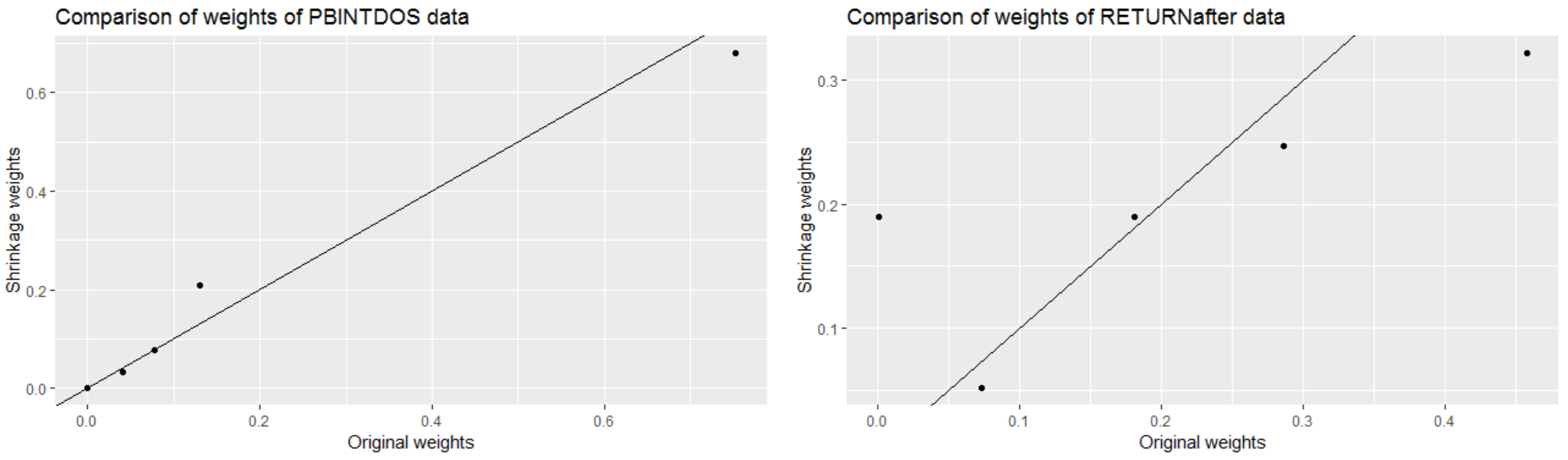
3.1. Deriving Weights Using 10 Seed Questions

Two data sets ($PBINTDOS$ and $RETURNafter$) were selected for the initial analysis. Data contained experts’ elicited 5%, 50% and 95% percentiles of the probability distributions of quantities corresponding to the seed questions in both data sets. The experts who answered the majority of seed questions were selected from each data set. Data from the first 35 seed questions from five experts with their expert IDs (from two to six) were selected from the $PBINTDOS$ data set. Data from all 31 seed questions and all five experts were used from the $RETURNafter$ data set. The first 10 questions of each data set were used to derive weights and the remaining questions were used to estimate variances of weights and to compare the overall calibration and informativeness scores of classical and shrinkage CM weights.

The Excalibur package was used to obtain the normalized CM weights of the DM from the training data. The version of the DM (used in this analysis) was the aggregation of all experts, without imposing a threshold value to include only experts whose calibration scores exceeded a certain cut-off value for allocating weights. Therefore, each expert’s distribution had a non-zero weight proportional to the expert’s combined score based on calibration and informativeness.

Results Addressing the First Research Question

To reiterate, the first research question was: can the shrinkage CM weights calculated from 10 seed questions improve the group’s aggregated probability distributions?

First, consider the analysis of the $PBINTDOS$ data. The seed questions were selected so that they were as similar as possible to the uncertain quantities of interest. As expected, the derived CM weights from different random samples from the seed testing questions were different even though they were derived from the same number of questions from the same background. The empirical Bayes shrinkage approach discussed helped us address the uncertainty in the weights.

The plot on the left hand side of Figure 1 compares the normalized classical and shrinkage CM weights from the $PBINTDOS$ training data. Each dot corresponds to one expert. There are some differences between weights for larger classical CM weights. A similar analysis was carried out, following the same procedure, for the $RETURNafter$ data set. The plot on the right hand side of Figure 1 shows that the classical and shrinkage CM weights are different for both larger and smaller classical weights. This demonstrates the impact of shrinking the CM weights considering their variability.

As expected, the sets of weights will be different and, theoretically, the shrinkage CM weights are better. We expect these differences to affect the performance of the calibration and informativeness of the DM for the testing data.

Table 2. Overall Decision Maker scores of testing questions.

Data Set	Types of Weight	Calibration Score	Information Score
PBINTDOS	Classical	0.7496	1.044
	Shrinkage	0.7587	1.077
RETURNafter	Classical	0.01487	0.2433
	Shrinkage	0.004452	0.2837

summarizes the DM scores for both testing data sets. While, for the $PBINTDOS$ data set, the DM calibration and information scores are slightly higher for the shrinkage weights compared with the classical weights, for the $RETURNafter$ data set, the shrinkage weights have produced a lower DM calibration but still a higher information score.

The above results are inconclusive when scrutinized from the DM performance perspective. Not only they did not behave consistently, but also, the magnitude of the differences between scores was completely irrelevant. For example, no real distinction can be made between a calibration of $0.75$ and one of $0.76$, especially when calculated on 10 calibration questions. Contrary to expectations, practically, we cannot yet observe an improvement in the DMs’ performance that will justify using the shrinkage weights. Such results, however, boost one’s confidence in current practices.

When more seed questions are used in the training set, the results remain as inconclusive as above. Two more data sets with a very large number of seed questions ($THRMBLD$ and $TNODISPR$) were selected for analysis using 20 seeds, and the results are presented in the Supplementary Material, as mentioned in Section 2.4 above.

Unfortunately, the investigated data sets are the only ones (to the authors’ knowledge) with enough seed questions to peruse this type of analysis further. However, the results above suggest that the DMs’ performance is not as sensitive as we expected to the unaccounted variance in weights. This suggests a different use (potentially more important from a practical perspective) of the proposed methodology, namely improving situations when fewer than the advised number of seed questions are available.

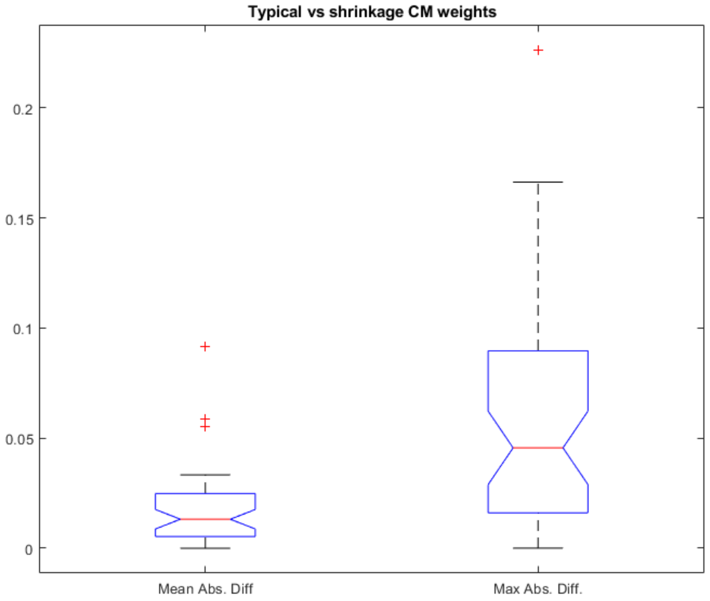
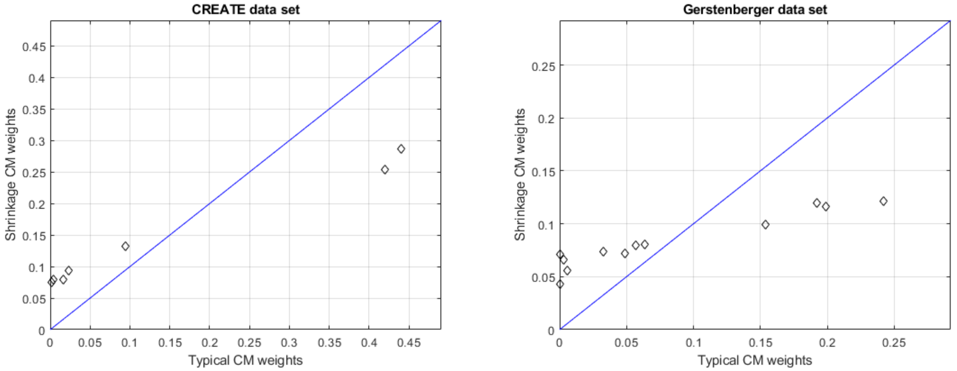
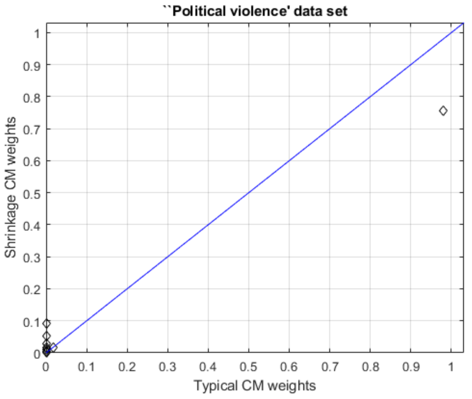
3.2. Deriving Weights Using Fewer than 10 Seed Questions

To tackle the conjecture formulated at the end of the previous section, we can in fact use a larger set of studies. For the 49 studies described in Section 2.3, we used the methodology detailed in Section 2.5 for all possible combinations of $N=10$ and $N=100$ samples; five and seven seed questions; and 2, 3 or $N-1$ degrees of freedom. All generated results tell a coherent story and are available upon request. The results presented here are the ones for 100 samples, seven seed variables and three degrees of freedom. The reason for the these choices are that we expect sampling 100 times to be more reliable than sampling only 10 times; 7 seed questions is a plausible situation (when 3 of the 10 asked were found to be unusable) and three degrees of freedom was one of the choices from Zhao [5].

Results Addressing the Second Research Question

It is worth reiterating that the classical CM weights are calculated using 10 seeds and the shrinkage weights use 7, but incorporate information about the weights’ variance.

Figure 2 shows the spread of the mean (per study) absolute difference between the weights and the spread of the maximum (per study) absolute difference. The median values of both these differences are below $0.05$, with the median average difference being $0.01$. These very low values, although expected, suggest that shrinkage weights calculated from a smaller number of seeds may potentially achieve very similar results when compared with the classical CM weights. A small number of seeds is not unusual in practical settings, and the above results suggest that applying the shrinkage technique could improve performance to the level of the best practice in terms of the number of seeds.

Before investigating how the difference in weights translates to the difference in the DMs’ performance, we note four outlier studies (corresponding to the four red crosses) for which larger differences were observed.

Figure 3 shows the weights calculated for two of the studies corresponding to the larger mean absolute difference. In both studies, all weights changed moderately: the largest classical weights are slightly reduced by shrinkage and the smallest weights become larger to compensate.

Figure 4 shows the outlier study in terms of the largest maximum difference. Here, only the maximum weight changes drastically and is being reduced by shrinkage, to be redistributed among the smaller weights.

Just as in the previous analysis, what we are interested in in practice is how different weights affect the performance of the DM. Figure 5 shows the calibration scores (lhs) and the informativeness scores (rhs) of the DMs calculated with 1) the classical DM weights based on 10 seeds (on the x-axis) and 2) the shrinkage DM weights calculated based on 7 seeds (on the y-axis).

The majority of the calibration score pairs are on the main diagonal, suggesting no change in performance. Moreover, the majority of the pairs that are not on the main diagonal are very small and within a restricted region around the main diagonal. This region is bounded by the two dashed lines. Akin to the discussion in Hanea and Nane [11], we consider scores within this region to represent equivalent performance. Interestingly, in two studies the shrinkage weights generate a much better calibration score for the DM. The informativeness scores tell a similar story, but in this case, the majority of scores are better when calculated with the classical weights. This is not surprising giving that extra calibration is usually obtained by losing informativeness.

4. Conclusions

Experts’ weights are derived from experiments to obtain aggregated probability distributions of unknown quantities. Therefore, they are random variables and should be treated as such. The focus of the present analysis was to address this underlying uncertainty of the derived experts’ weights from experiments in computing aggregated distributions of quantities. The James–Stein shrinkage estimation technique discussed in James and Stein [4] can be applied to estimate the mean of a multivariate normal distribution with reduced mean squared errors. An empirical Bayes development of the James–Stein shrinkage estimation technique discussed in Zhao [5] that shrinks variables differently depending on their variances was employed to derive weights in this analysis. Hence, larger shrinkage was applied to derived weights with larger variances.

If we consider the practical context of deriving experts’ weights, it can be observed that a small number of seed questions is used in general. While we acknowledge the potential difficulties of eliciting more seed questions, we would like to emphasize the unstable nature of the weights when calculated from a small set of seed questions. The variability in experts’ weights calculated using limited amounts of information (due to the lack of seed questions) is equated with deviation from the unknown mean values of the random distributions of weights. Therefore, the smaller the number of seed questions, the larger the variances in weights. We proposed deriving shrinkage weights to reduce the mean squared errors of estimated mean weights when a limited number of seed questions are used to derive these weights.

The results of our analysis show promise not only theoretically, but also from a practical perspective. Not having enough seed questions for a study can be remedied by shrinking the weights and achieving the same performance of the DM.

As a theoretical limitation, we can discuss one assumption needed during the estimation procedure proposed. When applying the double shrinkage estimator defined in Equation (4) in Section 2.2 to derive shrinkage weights, the original weights were assumed to be normally distributed. The original weights were, however, non-negative and, according to Equation (4), the resulting shrinkage weights were also non-negative. The assumption of normality for non-negative weights can be justified as follows. If we repeat the experiment a large number of times under similar conditions and observe the weights, then it is reasonable to assume a bell-shaped curve in general, as there will be more moderate values of weights in general, and few extreme values of weights in the right and left tails. In addition to that, theoretically, we consider the limits of a normal random variable to be negative and positive infinity. However, in this application (like in many others), the range of a given normal random variable can be restricted to a lower range considering the fact that almost all observations of a normal random variable remain within four standard deviation units from the mean. Thus, assuming a normal distribution for non-negative experts’ weights, even though not intuitive, can be justified.

In terms of practical limitations, we must acknowledge that additional sets of seed questions to estimate the sample variances of weights (to derive the shrinkage weights) may not be available in practice. However, $95\%$ of the estimated variances were less than $0.04$. A further analysis may need to investigate if a fixed variance can be used, or if any characteristics of an elicitation can explain different variances. Another potential approach would be to apply the non-parametric jackknife resampling method discussed in Efron and Stein [23] for estimating the variances of experts’ weights using a given set of seed questions. It allows the estimation of sample variances of weights for experts through separately derived weights from separate samples of seed questions that are obtained by applying the jackknife resampling method on a given set of seed questions.

The same jackknife resampling method may be used instead of the fourth step of the procedure from Section 2.4. This would correspond to relaxing the independence assumption in the double shrinkage procedure from Zhao [5] and developing a new robust shrinkage approach that allows for a general estimate of variances in weights. Another potential future direction of this study is investigating the variance in (and the potential shrinkage of) calibration scores rather than the variance in the weights.

References

1. O’Hagan, A. Expert Knowledge Elicitation: Subjective but Scientific. Am. Stat. 2019, 73, 69–81. [Google Scholar] [CrossRef]
2. Cooke, R. Experts in Uncertainty: Opinion and Subjective Probability in Science; Oxford University Press on Demand: Oxford, UK, 1991. [Google Scholar]
3. Stein, C. Inadmissibility of the usual estimator for the mean of a multivariate normal distribution. In Proceedings of the Third Berkeley Symposium on Mathematical Statistics and Probability, Berkeley, CA, USA, 26–31 December 1954; University of California Press: Berkeley, CA, USA, 1956; pp. 197–206. [Google Scholar]
4. James, W.; Stein, C. Estimation with quadratic loss. In Proceedings of the Fourth Berkeley Symposium on Mathematical Statistics and Probability, Berkeley, CA, USA, 20–30 July 1960; University of California Press: Berkeley, CA, USA, 1961; pp. 361–379. [Google Scholar]
5. Zhao, Z. Double shrinkage empirical Bayesian estimation for unknown and unequal variances. Stat. Its Interface 2010, 3, 533–541. [Google Scholar] [CrossRef]
6. Voinov, V.G.; Nikulin, M.S. A review of the results on the Stein approach for estimators improvement. Qüestiió 1995, 19, 1–3. [Google Scholar]
7. Cooke, R.M.; Wittmann, M.E.; Lodge, D.M.; Rothlisberger, J.D.; Rutherford, E.S.; Zhang, H.; Mason, D.M. Out-of-sample validation for structured expert judgment of Asian carp establishment in Lake Erie. Integr. Environ. Assess. Manag. 2014, 10, 522–528. [Google Scholar] [CrossRef] [PubMed]
8. Cooke, R.M.; Goossens, L.L. TU Delft expert judgment data base. Reliab. Eng. Syst. Saf. 2008, 93, 657–674. [Google Scholar] [CrossRef]
9. O’Hagan, A.; Buck, C.E.; Daneshkhah, A.; Eiser, J.R.; Garthwaite, P.H.; Jenkinson, D.J.; Oakley, J.E.; Rakow, T. Uncertain Judgements: Eliciting Experts’ Probabilities; John Wiley & Sons: Hoboken, NJ, USA, 2006. [Google Scholar]
10. Quigley, J.; Colson, A.; Aspinall, W.; Cooke, R.M. Elicitation in the Classical Model. In Elicitation: The Science and Art of Structuring Judgement; Dias, L.C., Morton, A., Quigley, J., Eds.; Springer International Publishing: Cham, Switzerland, 2018; pp. 15–36. [Google Scholar] [CrossRef]
11. Hanea, A.M.; Nane, G.F. An In-Depth Perspective on the Classical Model. In Expert Judgement in Risk and Decision Analysis; Hanea, A.M., Nane, G.F., Bedford, T., French, S., Eds.; International Series in Operations Research & Management Science; Springer: Berlin/Heidelberg, Germany, 2021; pp. 225–256. [Google Scholar] [CrossRef]
12. Efron, B.; Morris, C. Data analysis using Stein’s estimator and its generalizations. J. Am. Stat. Assoc. 1975, 70, 311–319. [Google Scholar] [CrossRef]
13. Kwon, Y.; Zhao, Z. On F-modelling-based empirical Bayes estimation of variances. Biometrika 2023, 110, 69–81. [Google Scholar] [CrossRef]
14. Wang, Z.; Lin, L.; Hodges, J.S.; MacLehose, R.; Chu, H. A variance shrinkage method improves arm-based Bayesian network meta-analysis. Stat. Methods Med. Res. 2021, 30, 151–165. [Google Scholar] [CrossRef] [PubMed]
15. Ragain, S.; Peysakhovich, A.; Ugander, J. Improving pairwise comparison models using empirical bayes shrinkage. arXiv 2018, arXiv:1807.09236. [Google Scholar]
16. Jing, B.Y.; Li, Z.; Pan, G.; Zhou, W. On sure-type double shrinkage estimation. J. Am. Stat. Assoc. 2016, 111, 1696–1704. [Google Scholar] [CrossRef]
17. Dharmarathne, H.A.S.G. Exploring the Statistical Aspects of Expert Elicited Experiments. Ph.D. Thesis, The University of Melbourne, Melbourne, VIC, Australia, 2020. [Google Scholar]
18. Eggstaff, J.W.; Mazzuchi, T.A.; Sarkani, S. The effect of the number of seed variables on the performance of Cooke’ s classical model. Reliab. Eng. Syst. Saf. 2014, 121, 72–82. [Google Scholar] [CrossRef]
19. Marti, D.; Mazzuchi, T.A.; Cooke, R.M. Are Performance Weights Beneficial? Investigating the Random Expert Hypothesis. In Expert Judgement in Risk and Decision Analysis; Hanea, A.M., Nane, G.F., Bedford, T., French, S., Eds.; Springer International Publishing: Cham, Switzerland, 2021; pp. 53–82. [Google Scholar] [CrossRef]
20. Cooke, R.M.; Marti, D.; Mazzuchi, T. Expert forecasting with and without uncertainty quantification and weighting: What do the data say? Int. J. Forecast. 2021, 37, 378–387. [Google Scholar] [CrossRef]
21. Cooke, R.M.; Solomatine, D. EXCALIBR Integrated System for Processing Expert Judgements Version 3.0; Delft University of Technology and SoLogic Delft: Delft, The Netherlands, 1992. [Google Scholar]
22. Colonna, K.J.; Nane, G.F.; Choma, E.F.; Cooke, R.M.; Evans, J.S. A retrospective assessment of COVID-19 model performance in the USA. R. Soc. Open Sci. 2022, 9, 220021. [Google Scholar] [CrossRef] [PubMed]
23. Efron, B.; Stein, C. The jackknife estimate of variance. Ann. Stat. 1981, 9, 586–596. [Google Scholar] [CrossRef]
Figure 1. Normalized classical and shrinkage CM weights.
Forecasting 05 00029 g001
Figure 2. Mean and maximum absolute differences between the classical and shrinkage CM weights.
Forecasting 05 00029 g002
Figure 3. Particular studies with large differences between the classical and shrinkage CM weights.
Forecasting 05 00029 g003
Figure 4. Particular study with the largest absolute differences between the classical and shrinkage CM weights.
Forecasting 05 00029 g004
Figure 5. The DMs’ performance when using classical and shrinkage weights.
Forecasting 05 00029 g005