A Mixture Integer GARCH Model with Application to Modeling and Forecasting COVID-19 Counts

Abstract

This article introduces a flexible time series regression model known as the Mixture of Integer-Valued Generalized Autoregressive Conditional Heteroscedasticity (MINGARCH). Mixture models provide versatile frameworks for capturing heterogeneity in count data, including features such as multiple peaks, seasonality, and intervention effects. The proposed model is applied to regional COVID-19 data from Malaysia. To account for geographical variability, five regions—Selangor, Kuala Lumpur, Penang, Johor, and Sarawak—were selected for analysis, covering a total of 86 weeks of data. Comparative analysis with existing time series regression models demonstrates that MINGARCH outperforms alternative approaches. Further investigation into forecasting reveals that MINGARCH yields superior performance in regions with high population density, and significant influencing factors have been identified. In low-density regions, confirmed cases peaked within three weeks, whereas high-density regions exhibited a monthly seasonal pattern. Forecasting metrics—including MAPE, MAE, and RMSE—are significantly lower for the MINGARCH model compared to other models. These results suggest that MINGARCH is well-suited for forecasting disease spread in urban and densely populated areas, offering valuable insights for policymaking.

1. Introduction

In epidemiology and infectious disease research, case counts are commonly used for analysis. For the past 40 years, the thinning operator in INAR model has been extensively adopted as a substitute for continuous multiplication in Box–Jenkins autoregressive moving average (ARMA) models. Ref. [1] were among the first to recommend thinning-based integer-valued time series models for epidemiology studies, highlighting their utility in infectious disease surveillance. The most common and fundamental integer-valued time series models are the integer-valued autoregressive (INAR) models. These models have gained considerable attention for modeling COVID-19 incidence since the onset of the pandemic. For instance, Refs. [2,3] examined the generalized non-linear state–space model for COVID-19 fatalities. Recently, Ref. [4] modelled the cumulative confirmed cases in Kenya with the negative binomial INAR (1) model, Ref. [5] applied zero-inflated Poisson time series, and Ref. [6] extended the analysis by using INAR (p) models. Although the application of integer-valued time series models to count data is well-established, there are differing opinions on their applicability to low count data Ref. [7]. Modeling COVID-19 incidence is challenging, in particular due to the high number of confirmed cases across countries. Ref. [8] considered the Poisson autoregressive model to understand the dynamics of disease contagion. The suitability of thinning-based integer-valued time series models for disease incidence is a contentious topic, particularly given the tendency for disease cases to exhibit seasonality and multiple peaks.

Many existing time series models for count data were generalized from the INAR models Ref. [9]. Other models to deal with count data include the discrete time series generated by mixture Ref. [10], the discrete-valued ARMA model Ref. [11], and the mixture of Pegram and thinning model Refs. [12,13]. Refs. [7,14] considered the model with low count and excess zero data, respectively. Most of these models assume a constant mean and variance, which failed to account for the seasonality or multiple peaks nature of infectious diseases. This paper provides a solution to cater for the seasonality and multiple peaks in the data by using a simple mathematical formulation with well-defined statistical properties. This is achieved by considering a mixing operator for the mean and variance function.

Ref. [15] introduced an analogue generalized autoregressive conditional heteroskedastic (GARCH) for integer values, namely INGARCH, to consider the random variables with non-constant mean function. The model is defined as follows:

Definition 1. (INGARCH)

Let $\left\{X_t\right\}$ be an integer-valued process regressed by a set of past observation ${\mathcal{F}}_{t-1}$ such that

$$X_t|{\mathcal{F}}_{t-1}~P\left({\kappa }_t\right),{\kappa }_t={\beta }_0+\sum _{i=1}^q{\beta }_i{X}_{t-i}+\sum _{j=1}^p{\alpha }_j{\kappa }_{t-j}$$

where $P\left({\kappa }_t\right)$  is a Poisson process with the parameter ${\kappa }_t$, ${\beta }_0>0,{\beta }_i\ge 0,i=1,...,q,{\alpha }_j\ge 0,j=1,...,p$.

The INGARCH model is an analogue of the GARCH model originally proposed by Ref. [16]. It was developed to enhance Engle’s ARCH model and is capable of modeling various economic phenomena. Notably, the INGARCH model incorporates a linear function for the mean parameter and serves as a regression model for count time series data. The model can accommodate data that exhibits heteroscedasticity and has been extended by Ref. [17] to handle data with intervention effects. The models were developed in R by Ref. [18], utilizing the tseries package. The model is applied to analyze the daily number of deaths due to COVID-19 in Ireland. Ref. [19] considered count regression models for eighteen countries worldwide, including Malaysia. The study assumes that the observation, regressed by the past observation, follows a Poisson or negative binomial distribution with the parameter estimated using a log-link linear equation.

Ref. [11] presented a discrete-valued time series based on Pegram’s operator Ref. [20], which is defined as follows.

Definition 2. (Pegram’s Mixture)

For two independent discrete random variables $U$ and $V$, and for a given mixing weight  $\varphi \in \left(\mathrm{0,1}\right)$, Pegram’s operator mixes  $U$ and $V$ with the respective mixing weights of $\varphi$ and $1-\varphi$, to produce a random variable

$$Z=\left(\varphi , U\right)\ast \left(1-\varphi , V\right)$$

(1)

with the marginal probability function given by

$$P\left(Z=j\right)=\varphi P\left(U=j\right)+\left(1-\varphi \right)P\left(V=j\right), j=\mathrm{0,1},2,\dots$$

In Equation (1), the domain of the random variables is $\{\mathrm{0,1},\dots \}$. This operator $\ast$ indicates a mixture of two discrete distributions and will be called the mixing operator. This model is applicable to non-infinitely divisible marginal distributions. Ref. [11] have illustrated an application of the model with categorical infant count data. Mixture models are simple in form and provide great flexibility to fit various characteristics of the data. In the continuous case, the mixture of distributions yields flexible time series models Refs. [21,22,23].

Refs. [12,13] developed an integer-valued time series model by combining mixture and thinning operators. The model is known as the mixture of Pegram and Thinning (MPT), which is expressed as

$$X_t=\left(\phi , \alpha \circ X_{t-1}\right)\ast \left(1-\phi , {\epsilon }_t\right)$$

where $\circ$ is the thinning operator and $\ast$ is the mixing operator. The thinning operator is defined as follows.

Definition 3. (Binomial Thinning)

Let $X$ be a non-negative integer-valued random variable. Then for any $\alpha \in \left(0, 1\right)$ the operator $’\circ ’$ is defined by

$$\alpha \circ X=\sum _{i=1}^X{Y}_i$$

(2)

where $Y_i$, with $E\left[Y_i\right]=\alpha , Var\left[Y_i\right]=\alpha (1-\alpha )$, is a sequence of independent and identically distributed (i.i.d.) Bernoulli random variables, independent of $X$, such that

$$P\left(Y_i=1\right)=\alpha =1-P(Y_i=0)$$

The first order MPT model is weakly stationary, and its complete statistical properties, including coherent forecasting Ref. [13], have been explored. This model is designed for count data with constant mean and variance. However, the MPT model performs poorly when the data presents seasonality patterns or multiple peaks which features commonly seen in infectious disease incidence, which makes modeling such data challenging. To address these shortcomings, this paper proposes a new integer-valued generalized autoregressive conditional heteroscedasticity (INGARCH) model with a mixture formulation, referred to as the Mixture INGARCH (MINGARCH) model, for modeling infectious disease incidence.

Compared to the INGARCH model by Ref. [15], and extended with intervention effects by Ref. [17], the MINGARCH model has a simpler mathematical expression, which facilitates its application not only in infectious diseases modeling, but also in other fields like economics and finance. The advantages of the model are demonstrated with better prediction results.

As of March 2023, the COVID-19 pandemic has caused over 9 million deaths worldwide, along with significant social and economic disruptions, including widespread job losses, business closures, and a global recession. Statistical modeling, especially time series analysis, plays a crucial role in understanding the spread of COVID-19 and assessing intervention strategies. Previous studies, such as Refs. [24,25], have applied ARIMA and other time series models to COVID-19 data. However, many traditional models, including the SIR model, may not adequately capture the unique nature of COVID-19 data, which is primarily count-based. This paper makes two key contributions. First, it introduces a new MINGARCH model, incorporating the Poisson process, to model confirmed COVID-19 cases in Malaysia from 1 March 2021 to 23 October 2022. Given the regional variation in disease incidence, five Malaysian regions were analyzed. There is limited literature on the region-specific analysis of COVID-19 incidence in Malaysia. It is shown that the MINGARCH model can effectively capture seasonality and intervention effects present in the selected duration. A comparative study with the INGARCH models Refs. [15,17] shows that the proposed model outperformed them. Second, for forecasting the MINGARCH model performed favorably. In a recent review on the application of machine learning methods to COVID-19 data analysis, Ref. [26] concluded that there is no single best-performing model; rather, different algorithms tend to perform better on different subsets of data or address different aspects of the problem more effectively. Among traditional time series models, ARIMA has been the most widely used, whereas in the domains of machine learning and deep learning, neural networks—particularly Long Short-Term Memory (LSTM) models—have seen the highest usage.

The paper is structured as follows. Section 2 presents the proposed model. Considerable effort has been devoted to the comprehensive study of the data, including an investigation of its characteristics such as spread and seasonality patterns. Section 2.2 provides a detailed analysis of the data, including its spread and seasonal characteristics. Section 3 discusses the results of model fitting and comparison. Section 4 concludes the analysis.

2. Materials and Methods

2.1. Mixture INGARCH Model

The mixture INGARCH model is defined as follows.

Definition 4.

Let ${\left\{X_t\right\}}_{t\in \mathbb{Z}}$ be an integer-valued generalized autoregressive conditional heteroscedastic (INGARCH) model defined by

$$X_t|{\mathcal{F}}_{t-1}~\mathrm{Poisson}({\mu }_t)$$

(3)

where the mean function ${\mu }_t$ follows Ref. [20]s mixture AR model, which is given by

$${\mu }_t=\left({1-\delta }_1-{\delta }_2-\cdots {\delta }_p\right){\mu }_{t-p}+{\varphi }_1{X}_{t-1}+\cdots +{\varphi }_q{X}_{t-q}$$

 where ${\delta }_i,{\varphi }_j\ge 0, (1-\sum _{i=1}^p{\delta }_i)+\sum _{j=1}^q{\varphi }_j=1.$

• This sequence ${\left\{X_t\right\}}_{t\in \mathbb{Z}}$ is known as a mixture INGARCH (MINGARCH) model.

The conditional probability mass function is simply a Poisson process given by

$$P\left(X_t|{\mathcal{F}}_{t-1}\right)={\displaystyle \frac{e^{-{\mu }_t}{\left({\mu }_t\right)}^{X_t}}{X_t!}}$$

The corresponding likelihood function is given by

$$L\left({\mu }_t,x_t\right)={\prod }_{t=1}^n\mathit{exp}\left(-{\mu }_t\right){\displaystyle \frac{{\left({\mu }_t\right)}^{x_t}}{x_t!}}$$

The log-likelihood function is

$$\log L\left({\mu }_t\right)=-n{\mu }_t-{\sum }_{t=1}^n\ln \left(x_t!\right)+\ln \left({\mu }_t\right)·{\sum }_{t=1}^n{x}_t$$

It has been noted that the likelihood function of the MINGARCH model shares similarities with INGARCH models, with the expression relying on the fundamental Poisson likelihood function. The mean and variance functions of the Poisson MINGARCH model offer meaningful interpretations in modeling COVID-19 confirmed cases in Malaysia. In this model, we illustrate the mean and variance parameters as a mixture of sequential random variables that incorporate both past observations and lag-driven observation. Maximum likelihood estimation is used to estimate the parameters. The log-likelihood function can be easily solved numerically by using the R 4.2.3 GenSA package. The initial values were obtained via method of moments, and the stopping criterion is ${10}^{-6}$.

Proposition 1 gave a necessary condition on the parameters for the process to be second-order stationary. Two polynomials are defined here. Let $D\left(B\right)=1-{\delta }_{1}B-\cdots -{\delta }_p{B}^p$ and $G\left(B\right)=1-{\varphi }_{1}B-\cdots -{\varphi }_q{B}^q$, where $B$ is backward shift operator. The mean function in Definition 4 is rewritten as

$${\mu }_t=\left(1-{\sum }_{i=1}^p{\delta }_i\right){\mu }_{t-i}+{\sum }_{j=1}^q{\varphi }_j{X}_{t-j}$$

(4)

in the proof of second-order stationarity in Proposition 1.

Proposition 1.

For a second-order stationary process ${\left\{X_t\right\}}_{t\in {\rm Z}}$ to satisfy (3), it is necessary that $0\le \sum _{j=1}^q{\varphi }_j+\sum _{i=1}^p{\delta }_i<1$.

Proof. 

Let $D\left(1\right)=\sum _{i=1}^p{\delta }_i<1$ and $G\left(1\right)=\sum _{j=1}^q{\varphi }_j<1$, for $D\left(z\right)$ to lie outside the unit root circle. The mean function (4) in terms of backward shift operator is

$${\mu }_t=D^{-1}\left(B\right)\left[{\varphi }_0+G\left(B\right)X_t\right]={\varphi }_0{D}^{-1}\left(1\right)+H\left(B\right)X_t,$$

where $H\left(B\right)=G\left(B\right)·D^{-1}\left(B\right)=\sum _{k=1}^{\mathrm{\infty }}{\phi }_k{B}^k$, where $\left|B\right|\le 1$, or equivalently, the power series ${\sum }_{k=0}^{\mathrm{\infty }}\left|{\phi }_k\right|<\mathrm{\infty }$, ${\phi }_0=1$ converges absolutely. Let ${\phi }_j$ be the coefficient of $z^j$ in the Taylor expansion of $G\left(z\right)/D\left(z\right)$. We have

$$\begin{gathered} \mu =E\left(X_t\right)=E\left[E\left(X_t|{\mathcal{F}}_{t-1}\right)\right] \\ =E\left[{\varphi }_0{D}^{-1}\left(1\right)+\sum _{j=1}^{\infty }{\phi }_j{X}_{t-j}\right] \\ ={\varphi }_0{D}^{-1}\left(1\right)+D^{-1}\left(1\right)·G\left(1\right)·E\left(X_{t-j}\right) \\ ={\varphi }_0{D}^{-1}\left(1\right)+D^{-1}\left(1\right)·G\left(1\right)·\mu \end{gathered}$$

which leads to

$$\mu ={\displaystyle \frac{{\gamma }_0}{D\left(1\right)-G\left(1\right)}}={\gamma }_0{\left(1-{\sum }_{i=1}^p{\delta }_i-{\sum }_{j=1}^q{\varphi }_j\right)}^{-1}={\gamma }_0{K}^{-1}\left(1\right).$$

where $K\left(1\right)=D\left(1\right)-G\left(1\right)>0$. Considering the above, the parameters ${\delta }_i, i=1,\dots ,p$ and ${\varphi }_j, j=1,\dots , q$ of the non-negative integer-valued process ${\left\{X_t\right\}}_{t\in \mathsf{{\rm Z}}}$, must satisfy necessarily the condition:

$$1-{\sum }_{i=1}^p{\delta }_i-{\sum }_{j=1}^q{\varphi }_j>0$$

This completes the proof. □

Note: A similar proof can be found in Ref. [15] here an alternative form of the model is presented.

Proposition 2. (Unconditional mean of the MINGARCH(p,q) Model).

Let $0\le \sum _{j=1}^q{\varphi }_i+\sum _{i=1}^p{\delta }_i<1$, the MINGARCH(p,q) model is second-order stationary and its unconditional mean is

$$\mu ={\displaystyle \frac{{\varphi }_0}{1-\sum _{i=1}^p{\delta }_i-\sum _{j=1}^q{\varphi }_j}}$$

• The proof is rather simple by considering the total law of expectation. It can be noticed that for the MINGARCH(1,1) process, the unconditional mean is

$$\mu ={\displaystyle \frac{{\varphi }_0}{1-{\delta }_1-{\varphi }_1}}$$

Proposition 3. (Unconditional variance of MINGARCH(1,1) Process)

Let ${\left\{X_t\right\}}_{t\in {\rm Z}}$ to satisfy Equation (3) with the $p=1$ and $q=1$, and Proposition 1; the variance is given by

$$Var\left(X_t\right)={\displaystyle \frac{\mu \left(1-{\left({\delta }_1+{\varphi }_1\right)}^2+{{\delta }_1}^2\right)}{1-{\left({\delta }_1+{\varphi }_1\right)}^2}}$$

Remark .

It should be noticed that the marginal distribution is not a Poisson process as the mean is not equal to the variance.

Proposition 4. (Autocorrelation function of MINGARCH(1,1) Process)

Let ${\left\{X_t\right\}}_{t\in {\rm Z}}$ to satisfy Equation (3) with the $p=1$ and $q=1$, and Proposition 1; the autocovariance function is given by

$$Corr\left(X_t, X_{t-s}\right)={\left({\varphi }_1+{\delta }_1\right)}^{s-1}{\displaystyle \frac{{\varphi }_1\left(1-{\delta }_1\left({\varphi }_1+{\delta }_1\right)\right)}{1-{\left({\varphi }_1+{\delta }_1\right)}^2+{{\varphi }_1}^2}}$$

Corollary 1.

Let ${\left\{{\mathit{X}}_{\mathit{t}}\right\}}_{\mathit{t}\in \mathit{{\rm Z}}}$ satisfy Equation (3) with $\mathit{p}=1,\mathit{q}=1$, and the assumption that ${\mathit{\delta }}_1=1-{\mathit{\varphi }}_1$, then ${\left\{{\mathit{X}}_{\mathit{t}}\right\}}_{\mathit{t}\in \mathit{{\rm Z}}}$ is an INGARCH(1,1) process.

2.2. Covid Data

Malaysia’s first COVID-19 case was confirmed on 25th January 2020, with peaks of 5728 cases in January 2021 and 33,000 in March 2022, likely due to the Chinese New Year. This study models COVID-19 trends using data from March to October 2021, focusing on Selangor, Kuala Lumpur, Johor, Penang, and Sarawak. Figure 1 shows the time series plot of confirmed cases in five states in Malaysia. They are Johor, Selangor, Kuala Lumpur (KL), Penang, and Sarawak. The Selangor data indicates regional seasonality in a certain duration and presents two peaks in August 2021 and April 2022. This is because of the reopening after the movement control order (MCO) and the Chinese New Year celebration, respectively. It can be observed that the distribution patterns for KL and Selangor are similar, with a smaller scale of distribution found for the KL state. The confirmed cases for other states such as Penang and Sarawak also show dual peaks. Hence, it is believed that the new MINGARCH model is applicable for the data.

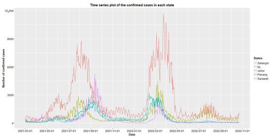
Figure 1. Time series plot of the confirmed cases.

The proposed MINGARCH model is compared with the following time series regression models:(1) Ref. [15], and (2) Ref. [17]. Figure 2 shows the frequency distribution of the confirmed cases in Selangor. The histogram of the data shows bimodality, which suggests that a mixture fitting is feasible.

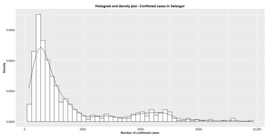
Figure 2. Frequency distribution of the number of confirmed cases in Selangor.

2.2.1. Descriptive Statistics

Table 1 presents the descriptive statistics for the COVID-19 dataset from 1 March 2021 to 23 October 2022, covering 86 weeks. Selangor reported the highest confirmed cases, with a peak exceeding 10,000 due to its large population and high mobility as a business hub. In contrast, Penang, despite its high population density, had lower confirmed cases, attributed to the state government’s stringent regulations and active disinfection efforts by local councils. Sarawak, with a lower population density, experienced a peak of about 5000 cases, considered severe given its vast land area. This study aims to investigate the MINGARCH model’s effectiveness in analyzing diverse data patterns, including population density. Table 1 outlines the statistics for the selected Malaysian states.

Table 1. Descriptive statistics.

State (Density)	Weekday	Descriptive Statistics
		Minimum	Q1	Median	Mean	Q3	Maximum
Selangor (880 km2)	Sunday	256	746	1112	2192	2330	9273
	Monday	213	613	884	1830	2096	6941
	Tuesday	242	663	1090	2079	2576	8095
	Wednesday	294	854	1436	2460	2809	10,240
	Thursday	237	892	1440	2537	2843	11,692
	Friday	348	822	1325	2600	2842	10,842
	Saturday	283	789	1394	2483	2754	10,790
KL (8157 km2)	Sunday	55	221	354	543	616	2685
	Monday	57	190	315	479	582	2214
	Tuesday	53	317	424	757	989	4527
	Wednesday	42	320	455	745	961	3565
	Thursday	79	334	517	770	976	3266
	Friday	86	308	484	783	966	4105
	Saturday	67	298	476	711	773	3603
Penang (1664 km2)	Sunday	57	140	216	427	422	1961
	Monday	50	104	172	411	398	2137
	Tuesday	53	115	199	473	421	2601
	Wednesday	51	119	198	498	430	2575
	Thursday	65	143	234	527	481	2773
	Friday	75	140	248	519	504	2750
	Saturday	74	134	218	494	407	2621
Johor (209 km2)	Sunday	28	87.5	354	573	728	2644
	Monday	36	92.8	340	577	757	2800
	Tuesday	29	91.5	348	564	665	2780
	Wednesday	33	103	384	606	700	2986
	Thursday	37	110	412	650	801	2856
	Friday	33	106	389	612	718	2860
	Saturday	33	81.2	403	592	710	3238
Sarawak (20 km2)	Sunday	6	51.2	234	507	580	5291
	Monday	7	39.2	213	464	521	3714
	Tuesday	10	79.8	211	505	605	3732
	Wednesday	13	81.2	212	513	549	4709
	Thursday	14	70.5	280	528	604	3660
	Friday	11	69	234	556	692	3734
	Saturday	13	56.2	238	504	570	3743

2.2.2. Data Properties

Hypothesis tests are carried out to test stationarity and seasonality. For the data duration, it is found that the data indicate a seasonality pattern. The Friedman test as suggested by Ref. [27] is applied to test seasonality. The hypotheses for the Friedman test are as follows:

$$\begin{gathered} H_0: \mathrm{no} \mathrm{stable} \mathrm{seasonality} \\ {H}_1: \mathrm{stable} \mathrm{seasonality} \end{gathered}$$

The seasonal test is tested at two significant levels, that is, 0.05 and 0.1. At 5% significant level, all states reject the null hypothesis except KL. At 10% significant level, it is seen that all states reject the null hypothesis. Therefore, we conclude that the seasonality is observed for all states at 10% significant level. Table 2 shows the decision and the conclusion of the Friedman test for all states. Next, besides the stationarity test, the sample autocorrelation function (ACF) served as an indicator for stationarity. Damped oscillation is observed in the sample ACF plots for all the states to indicate stationarity.

Table 2. Decision of the Friedman test.

State	Decision	Conclusion of Seasonality Indicator
Selangor	Reject	at lags 18, 33 to 39
KL	Reject	at lags 18, 27, 28 and 34
Johor	Reject	at lags 21 to 24
Penang	Reject	at lags 13, 22 to 26
Sarawak	Reject	at lags 21 to 27

3. Results and Discussion

3.1. Model Fitting

The data is fitted to all models provided in Section 3, MINGARCH, INGARCH [8], and INGARCH with intervention Ref. [17] models. The data is fitted to the MINGARCH model. We compared the model fitting with Refs. [15,17] with the suggested lags by the MINGARCH model. The results are tabulated in Table 3, Table 5 and Table 6. The Friedman test is applied to suggest the size for seasonality. The loglikelihood values, Akaike information criterion (AIC), and Bayesian information criterion (BIC) are calculated for model selection.

Table 3 shows the fits for the MINGARCH model. The Friedman test detects that the seasonal size of Selangor, KL, and Penang is 34 weeks, with the same order sizes of 3. Also, the sample autocorrelation functions in Figure 3 provides similar suggestion. While the state of Johor and Selangor show seasonal sizes of 24 weeks and 23 weeks, respectively.

Table 3. Loglikelihood, AIC, and BIC values for MINGARCH model.

State	Seasonal Size	Order Size	Loglikelihood	AIC	BIC
Selangor	34	3	−10,693	21,395	21,404
KL	34	3	−3462	6932	6941
Johor	24	1	−17,000	34,004	34,008
Penang	34	3	−13,950	27,909	27,918
Sarawak	23	1	−29,690	59,384	59,388

Table 3. Loglikelihood, AIC, and BIC values for MINGARCH model.

State	Seasonal Size	Order Size	Loglikelihood	AIC	BIC
Selangor	34	3	−10,693	21,395	21,404
KL	34	3	−3462	6932	6941
Johor	24	1	−17,000	34,004	34,008
Penang	34	3	−13,950	27,909	27,918
Sarawak	23	1	−29,690	59,384	59,388

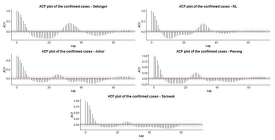
Figure 3. Sample ACFs and the 95% confidence interval (dotted line) of the confirmed cases for all states.

The seasonal pattern of COVID-19 repeats every 34 weeks in the states with high population density. For the states with huge land masses and relatively lower population densities, the COVID-19 has a repetitive peak about every 24 weeks.

Figure 3 shows the ACF plots for the five regions, which show strong autocorrelation at lag 1, indicating high temporal dependence in the confirmed COVID-19 cases. Selangor, Kuala Lumpur, and Johor exhibit periodic patterns and slow decay, suggesting seasonality and persistent transmission trends. Penang shows moderate autocorrelation with a weaker cyclical pattern, while Sarawak displays a sharp drop in autocorrelation, indicating less persistence. These differences highlight the need for region-specific modeling approaches. Regions with pronounced cyclic behavior may benefit from models incorporating seasonal or long-memory components, whereas simpler models may be sufficient for regions like Sarawak with faster autocorrelation decay. The orders and lags have been chosen based on the analysis, and the estimated parameters (standard errors) and mean function representative for respective states is tabulated in Table 4.

Table 4. The estimated parameters (standard errors) and the mean function for the states.

State	Mean Function
Selangor	${\mu }_t=0.1344 \left(0.0005\right){\mu }_{t-3}+0.8072\left(0.0018\right)Y_{t-3}$
KL	${\mu }_t=0.1162 \left(0.0018\right){\mu }_{t-3}+0.8513 \left(0.0047\right)Y_{t-3}$
Johor	${\mu }_t=0.3838 \left(0.0012\right){\mu }_{t-1}+0.4190{ \left(0.0014\right)Y}_{t-1}$
Penang	${\mu }_t=0.5454 \left(0.0021\right){\mu }_{t-3}+0.3284\left(0.0010\right)Y_{t-3}$
Sarawak	${\mu }_t=0.6032 \left(0.0014\right){\mu }_{t-1}+0.1255 \left(0.0003\right)Y_{t-1}$

Table 4. The estimated parameters (standard errors) and the mean function for the states.

State	Mean Function
Selangor	${\mu }_t=0.1344 \left(0.0005\right){\mu }_{t-3}+0.8072\left(0.0018\right)Y_{t-3}$
KL	${\mu }_t=0.1162 \left(0.0018\right){\mu }_{t-3}+0.8513 \left(0.0047\right)Y_{t-3}$
Johor	${\mu }_t=0.3838 \left(0.0012\right){\mu }_{t-1}+0.4190{ \left(0.0014\right)Y}_{t-1}$
Penang	${\mu }_t=0.5454 \left(0.0021\right){\mu }_{t-3}+0.3284\left(0.0010\right)Y_{t-3}$
Sarawak	${\mu }_t=0.6032 \left(0.0014\right){\mu }_{t-1}+0.1255 \left(0.0003\right)Y_{t-1}$

Model comparison has been carried out among MINGARCH, INGARCH, and INGARCH with intervention effect. The results are tabulated in Table 5 and Table 6, respectively. For the states of Selangor and KL, the AIC and BIC values of the MINGARCH model are lower compared to INGARCH and INGARCH with the intervention effect. For the state of Penang, the fits are competitive. However, the MINGARCH model does not perform well for the states of Johor and Sarawak with relatively low population density. It can be concluded that the MINGARCH model is suitable for model fitting for states with high population density, such as KL and Selangor. The higher population density may produce a larger seasonal size. Therefore, it may take longer to reach another repetitive seasonal peak. For instance, KL is foreseen to reach another peak of confirmed cases in about half a year. Based on the analysis, preventive measures or control can be carried out before the subsequent wave hit, especially in the high population density region. The next subsection examines forecasting performance for all the models considered here.

Table 5. Loglikelihood, AIC, and BIC values for INGARCH model.

State	Seasonal Size	Order Size	Loglikelihood	AIC	BIC
Selangor	34	3	−53,140	106,289	106,300
KL	34	3	−13,600	27,211	27,222
Johor	24	1	−5959	11,924	11,931
Penang	34	3	−13,797	27,603	27,614
Sarawak	23	1	−3882	7769	7776

Table 5. Loglikelihood, AIC, and BIC values for INGARCH model.

State	Seasonal Size	Order Size	Loglikelihood	AIC	BIC
Selangor	34	3	−53,140	106,289	106,300
KL	34	3	−13,600	27,211	27,222
Johor	24	1	−5959	11,924	11,931
Penang	34	3	−13,797	27,603	27,614
Sarawak	23	1	−3882	7769	7776

Table 6. Loglikelihood, AIC, and BIC values for INGARCH model with intervention effect.

State	Seasonal Size	Order Size	Loglikelihood	AIC	BIC
Selangor	34	3	−50,601.131	101,216	101,232
KL	34	3	−13,549.302	27,113	27,128
Johor	24	1	−12,907.852	25,826	25,837
Penang	34	3	−14,449.323	28,913	28,928
Sarawak	23	1	−2784.7142	5579	5591

Table 6. Loglikelihood, AIC, and BIC values for INGARCH model with intervention effect.

State	Seasonal Size	Order Size	Loglikelihood	AIC	BIC
Selangor	34	3	−50,601.131	101,216	101,232
KL	34	3	−13,549.302	27,113	27,128
Johor	24	1	−12,907.852	25,826	25,837
Penang	34	3	−14,449.323	28,913	28,928
Sarawak	23	1	−2784.7142	5579	5591

3.2. Forecasting

This subsection discusses the forecasting results for all three models, that is, MINGARCH, INGARCH, and INGARCH with intervention effect. The forecasting performance is measured by mean absolute percentage error (MAPE), mean absolute error (MAE), and root mean squared error (RMSE). The data has been split into 80% training data and 20% testing data. The results show that the new MINGARCH model overall outperformed its counterparts. The values of MAPE, MAE, and RMSE are much lower compared to the others, except for the state of Sarawak. In Sarawak where the population is less dense at a particular area and more isolated in many suburbs, the transmission dynamics appear more stable and less influenced by short-term fluctuations. This is likely why the intervention effects model is a more appropriate fit for the data. This suggests that external interventions or regime shifts played a more dominant role in shaping the dynamics of confirmed cases. In contrast, for Johor, Penang, and Selangor states, the study has found that the forecasting results obtained from the MINGARCH model are significantly superior to those of the other models. The common characteristics of these states are highly population density, urbanization- and economy-focused, and presence of industrial and migrant workforce. It is found that MINGARCH is capable of handling the confirmed cases in the region with these characteristics, with high volatility of daily confirmed cases. It is worthwhile to take note of the large MAPE values in Johor and Penang. This is likely due to high volatility reported in daily counts. MAPE is known to be sensitive to small denominators, when the actual counts are low or near zero and will give large percentage deviations, even when MAE and RMSE remain moderate. Table 7 tabulates the forecasting performance for all models.

Table 7. Forecasting results for all models.

State	MINGARCH			INGARCH			INGARCH with Intervention
	MAPE	MAE	RMSE	MAPE	MAE	RMSE	MAPE	MAE	RMSE
Selangor	42.75	292.06	328.79	203.65	1359.59	1503.41	346.49	2488.56	2540.63
KL	38.80	336.18	458.25	47.21	294.56	340.00	83.82	374.29	442.69
Johor	400.85	266.94	268.22	576.54	356.35	415.69	805.51	525.15	548.79
Penang	262.04	252.94	257.39	512.88	439.24	526.84	580.98	481.97	600.75
Sarawak	195.92	135.59	137.53	154.75	118.29	163.33	116.04	89.41	118.81

3.3. Policy Implications

For effective policymaking, the findings highlight the critical need for region-specific intervention strategies that are directly informed by the modeled transmission dynamics. The MINGARCH model estimates reveal varying lag dependencies across regions, indicating different epidemic rhythms and behavioral responses. In highly populated regions like Selangor and Kuala Lumpur, the strong influence of lagged cases, particularly at a three-week interval, suggests a cyclical transmission pattern. This implies that interventions such as targeted testing, temporary mobility restrictions, or public advisories should be deployed proactively on a rolling three-week basis to preempt potential surges. Early warnings and flexible containment strategies are essential in these regions.

In contrast, Johor’s short-term dependence structure, with significant weight on 1-week lagged cases and means, highlights a reactive dynamic, were real-time surveillance and rapid response systems, pop-up testing centers, and adaptive vaccination campaigns can effectively dampen spikes. For Sarawak, the model indicates a stronger reliance on past mean values and a weaker dependence on lagged observed cases. This points to a gradual and persistent transmission pattern, where short-term interventions may have limited impact. Instead, policies should focus on long-term preventive measures, such as sustained community engagement, continuous public health education, and capacity-building for rural health infrastructure. These differentiated patterns demonstrate the practical value of statistical modeling in forming targeted public health policies. By integrating model-based insights such as lag structure, autocorrelation patterns, and overdispersion, policymakers can optimize resource allocation, align interventions with epidemiological realities, and improve the timing and precision of public health responses across regions.

4. Concluding Remarks

This paper presents two contributions. Firstly, a new mixture time series regression model called MINGARCH has been introduced to fit regional COVID-19 data in Malaysia. Secondly, it has been observed that the MINGARCH model performs well in regions with high population density. The study has also established that the seasonal size of COVID-19 is proportional to the population density, which means that larger seasonal sizes may require a longer duration to reach the subsequent peak. The statistical analysis demonstrated that the MINGARCH model outperformed existing regression time series models, and its forecasting results were more promising. Overall, these findings highlight the potential usefulness of the MINGARCH model for application in infectious disease control measures.

References

- Cardinal, M.; Roy, R.; Lambert, J. On the application of integer-valued time series models for the analysis of disease incidence. Stat. Med. 1999, 18, 2025–2039. [Google Scholar] [CrossRef]
- Oustaloup, A.; Levron, F.; Victor, S.; Dugard, L. Non-integer (or fractional) power model of a viral spreading: Application to the COVID-19. Annu. Rev. Control 2021, 51, 324–334. [Google Scholar]
- Palmer, W.R.; Davis, R.A.; Zheng, T. Count-valued time series models for COVID-19 daily death dynamics. Stat 2021, 10, e369. [Google Scholar] [CrossRef] [PubMed]
- Wamwea, C.; Mwelu, S.; Odin, M. Modelling COVID-19 cumulative number of cases in Kenya using a negative binomial INAR(1) model. Open J. Model. Simul. 2023, 11, 14–36. [Google Scholar] [CrossRef]
- Tawiah, K.; Iddrisu, W.A.; Asosega, K.A. Zero-inflated time series modelling of COVID-19 deaths in Ghana. J. Environ. Public Health 2021, 2021, 5543977. [Google Scholar] [CrossRef] [PubMed]
- Soobhug, A.D.; Jowaheer, H.; Mamode Khan, N.; Reetoo, N.; Meethoo-Badulla, K.; Musango, L. Re-analyzing the SARS-CoV-2 series using an extended integer-valued time series models: A situational assessment of the COVID-19 in Mauritius. PLoS ONE 2022, 17, e0263515. [Google Scholar] [CrossRef]
- Freeland, R.K.; McCabe, B.P.M. Analysis of low count time series data by Poisson autoregression. J. Time Ser. Anal. 2004, 25, 701–722. [Google Scholar] [CrossRef]
- Agosto, A.; Giudici, P. A Poisson autoregressive model to understand COVID-19 contagion dynamics. Risks 2020, 8, 77. [Google Scholar] [CrossRef]
- Weiss, C.H. An Introduction to Discrete-Valued Time Series; Wiley: Hoboken, NJ, USA, 2018; ISBN 978-1-119-09696-2. [Google Scholar]
- Jacobs, P.A.; Lewis, P.A.W. Discrete time series generated by mixtures. I: Correlational and runs properties. J. R. Stat. Soc. Ser. B 1978, 40, 94–105. [Google Scholar] [CrossRef]
- Biswas, A.; Song, P.X.-K. Discrete-valued ARMA processes. Stat. Probab. Lett. 2009, 79, 1884–1889. [Google Scholar] [CrossRef]
- Khoo, W.C.; Ong, S.H.; Biswas, A. Modeling time series of counts with a new class of INAR(1) model. Stat. Pap. 2017, 58, 393–416. [Google Scholar] [CrossRef]
- Khoo, W.C.; Ong, S.H.; Atanu, B. Coherent forecasting for a mixed integer-valued time series model. Mathematics 2022, 10, 2961. [Google Scholar] [CrossRef]
- Khendhiri, S. Statistical modeling of COVID-19 deaths with excess zero counts. Epidemiol. Methods 2021, 10, 20210007. [Google Scholar] [CrossRef]
- Ferland, R.; Latour, A.; Oraichi, D. Integer-valued GARCH process. J. Time Ser. Anal. 2006, 27, 923–942. [Google Scholar] [CrossRef]
- Bollerslev, T. Generalized autoregressive conditional heteroskedasticity. J. Econom. 1986, 31, 307–327. [Google Scholar] [CrossRef]
- Fokianos, K.; Fried, R. Interventions in INGARCH processes. J. Time Ser. Anal. 2010, 31, 210–225. [Google Scholar] [CrossRef]
- Liboschik, T.; Fokianos, K.; Fried, R. tscount: An R package for analysis of count time series following generalized linear models. J. Stat. Softw. 2017, 82, 1–51. [Google Scholar] [CrossRef]
- Chan, S.; Chu, J.; Zhang, Y.; Nadarajah, S. Count regression models for COVID-19. Phys. A Stat. Mech. Appl. 2021, 563, 125460. [Google Scholar] [CrossRef]
- Pegram, G.G.S. An autoregressive model for multileg Markov chains. J. Appl. Probab. 1980, 17, 350–362. [Google Scholar] [CrossRef]
- Li, G.; Zhu, Q.; Liu, Z.; Li, W.K. On mixture double autoregressive time series models. J. Bus. Econ. Stat. 2017, 35, 306–317. [Google Scholar] [CrossRef]
- Low, V.J.M.; Khoo, W.C.; Khoo, H.L. A generalized Burr mixture autoregressive models for modeling non-linear time series. Commun. Stat. Theory Methods 2024, 53, 6832–6851. [Google Scholar] [CrossRef]
- Wong, C.S.; Chan, W.S.; Kam, P.L. A Student t-mixture autoregressive model with applications to heavy-tailed financial data. Biometrika 2009, 96, 751–760. [Google Scholar] [CrossRef]
- Golinski, A.; Spencer, P. Modeling the COVID-19 epidemic using time series econometrics. Health Econ. 2021, 30, 2808–2828. [Google Scholar] [CrossRef]
- Vig, V.; Kaur, A. Time series forecasting and mathematical modeling of COVID-19 pandemic in India: A developing country struggling to cope up. Int. J. Syst. Assur. Eng. Manag. 2022, 13, 2920–2933. [Google Scholar] [CrossRef]
- Cheng, Y.; Cheng, R.; Xu, T.; Tan, X.; Bai, Y. Machine learning techniques applied to COVID-19 prediction: A systematic literature review. Bioengineering 2025, 12, 514. [Google Scholar] [CrossRef]
- Demšar, J. Statistical comparisons of classifiers over multiple data sets. J. Mach. Learn. Res. 2006, 7, 1–30. [Google Scholar]
Disclaimer/Publisher’s Note: The statements, opinions and data contained in all publications are solely those of the individual author(s) and contributor(s) and not of MDPI and/or the editor(s). MDPI and/or the editor(s) disclaim responsibility for any injury to people or property resulting from any ideas, methods, instructions or products referred to in the content. |
© 2025 by the authors. Licensee MDPI, Basel, Switzerland. This article is an open access article distributed under the terms and conditions of the Creative Commons Attribution (CC BY) license (https://creativecommons.org/licenses/by/4.0/).