Kalman Filter-Based Real-Time Implementable Optimization of the Fuel Efficiency of Solid Oxide Fuel Cells

Abstract

The electric power characteristic of solid oxide fuel cells (SOFCs) depends on numerous influencing factors. These are the mass flow of supplied hydrogen, the temperature distribution in the interior of the fuel cell stack, the temperatures of the supplied reaction media at the anode and cathode, and—most importantly—the electric current. Describing all of these dependencies by means of analytic system models is almost impossible. Therefore, it is reasonable to identify these dependencies by means of stochastic filter techniques. One possible option is the use of Kalman filters to find locally valid approximations of the power characteristics. These can then be employed for numerous online purposes of dynamically operated fuel cells such as maximum power point tracking or the maximization of the fuel efficiency. In the latter case, it has to be ensured that the fuel cell operation is restricted to the regime of Ohmic polarization. This aspect is crucial to avoid fuel starvation phenomena which may not only lead to an inefficient system operation but also to accelerated degradation. In this paper, a Kalman filter-based, real-time implementable optimization of the fuel efficiency is proposed for SOFCs which accounts for the aforementioned feasibility constraints. Essentially, the proposed strategy consists of two phases. First, the parameters of an approximation of the electric power characteristic are estimated. The measurable arguments of this function are the hydrogen mass flow and the electric stack current. In a second stage, these inputs are optimized so that a desired stack power is attained in an optimal way. Simulation results are presented which show the robustness of the proposed technique against inaccuracies in the a-priori knowledge about the power characteristics. For a numerical validation, three different models of the electric power characteristic are considered: (i) a static neural network input/output model, (ii) a first-order dynamic system representation and (iii) the combination of a static neural network model with a low-order fractional differential equation model representing transient phases during changes between different electric operating points.

1. Introduction

Solid oxide fuel cell (SOFC) systems [1,2,3,4,5,6,7,8] are promising options for the design and implementation of a decentralized supply of consumers with both electric and thermal energy [9,10,11,12]. Such kinds of decentralized supply cannot only be realized in scenarios in which the produced electric power is fed into an existing grid (serving as a practically infinitely large storage from the point of view of a single fuel cell systems). Further configurations can also be investigated in isolated applications where the consumers are not directly connected to an electric power grid. This second option is especially interesting for the power supply of construction sites (for example, when building up new wind farms) or when the power supply of individual houses in small mountain and island villages is of interest. To some extent, electric energy buffers will be installed in such settings, where the storage can be achieved by super capacitors and (Lithium-ion) batteries if short and mid-term time scales are of interest.

However, the installation of each storage system introduces additional cost and components which are themselves subject to wear. The extent of the arising wear effects depends on operating strategies which impose constraints on the charging and discharging rates as well as the depth of discharge. For that reason, it is interesting to operate high-temperature fuel cells such as SOFCs not only at a fixed, offline-optimized operating point but with dynamically varying load conditions [13,14]. Such dynamic operating strategies will allow a downsizing of the aforementioned electric energy storage components.

For that purpose, two fundamental prerequisites need to be considered. First, the corresponding operating strategy needs to be able to make sure that the SOFC stack module is operated at a nearly constant temperature despite variable electric load conditions. This can be achieved by robust control strategies for the system’s thermal behavior [15,16,17,18]. Typically, the enthalpy flow of the supplied cathode gas is used as the corresponding control input for this purpose. In most cases, this enthalpy flow controller is implemented in such a way that the temperature of the cathode gas at the SOFC inlet manifold is manipulated. Suitable options—that are applicable over a wide range of operating conditions—make use of model-based feedback-linearizing approaches or sliding mode techniques. If these are combined with state and disturbance observers to estimate the temperature distribution in the interior of the SOFC stack (represented typically by a finite volume model) and to determine the values of disturbance heat flows and model deviations in terms of additive input variables, both of them can be made robust against parameter uncertainty. A guaranteed proof of stability can be achieved by a combination of Lyapunov techniques with tools from the area of interval analysis. Together, they allow for a guaranteed offline and online stabilization of the system dynamics if relevant parameters and measured quantities are known up to finitely large tolerance bounds [19,20,21]. Besides these approaches, very recent techniques for a robust control which combine interval methods with fuzzy techniques in terms of the so-called type-2 interval approach can be found in [22,23,24]. So far, these techniques have been mostly applied to proton-exchange membrane (PEM) fuel cells. However, from a methodological point of view, it may be interesting to compare them in future work with the previously mentioned references that use classical interval methods in the frame of SOFCs.

Despite these robust temperature control strategies, temperature variations in the range of several Kelvin occur inevitably in the interior of an SOFC stack which have a certain impact on the efficiency of the electric power production. This also holds for the influence of the stack inlet temperature on the electric power characteristic. In previous work, it was therefore proposed to represent the electric power characteristic in a model-free manner by a current-dependent polynomial [25]. However, the coefficients of this polynomial were not set to constant values but rather estimated during system operation by the application of a Kalman filter [26,27]. In general, Kalman filters are optimal, minimum variance state estimators for linear dynamic system models that are influenced additively by Gaussian process and measurement noise. Under these assumptions, a Kalman filter provides the possibility to estimate the expected values and covariances of the Gaussian probability densities of the state variables. Based on these estimates, numerous control approaches have been implemented in recent years. The most well-known technique is the combination of Kalman filters with state feedback controllers that are parameterized by the minimization of a quadratic cost function. This cost function takes into account a weighted superposition of state tracking errors and the required control effort and is typically referred to as LQR design [27,28].

For the online identification of the electric power characteristic of SOFCs, the Kalman filter makes use of the terminal voltage and terminal current of the SOFC stack as the measured parameters. The influence of the thermal operating point, gas mass flow and current dependencies on the electric power of the SOFC stack cannot be described perfectly by the assumed polynomial ansatz in [25]. Therefore, they are dealt with by adapting the polynomial’s coefficients in an online, real-time implementable manner by means of the Kalman filter in [25]. The estimation results then provided the required information to derive a maximum power point tracking procedure that uses the electric current as the control variable.

In this paper, the Kalman filter-based online identification scheme from [25] is extended toward not only estimating current dependencies but also for quantifying the effect of hydrogen gas mass flow variations. This latter extension is crucial for the derivation of control procedures that do not only adjust the terminal current to achieve a certain (maximum) power but also restrict the current such that overshooting the maximum power point is prevented and the system is guaranteed to be operated in the region of Ohmic polarization. In addition to current variations, the hydrogen mass flow will be adjusted systematically with the help of the Kalman filter’s estimation results. In summary, it becomes possible to optimize the fuel efficiency while simultaneously achieving a certain electric power as the system output under the constraint of preventing an overshoot of the maximum power point.

This paper is structured as follows. In Section 2, a summary of three structurally different simulation models for the electric power characteristic of an SOFC stack is presented. These simulation models differ in both their accuracy and complexity. In this paper, they are used to mimic different relations between the electric stack current and the hydrogen mass flow as the system inputs (together with further temperature-induced disturbances) to validate the proposed strategy for the online optimization of fuel efficiency. This strategy is based on the online identification of the electric power characteristic of an SOFC according to Section 3. This estimation scheme is then extended in Section 4 toward a real-time implementable current and hydrogen mass flow optimization. This optimization aims at an improved fuel efficiency and simultaneously ensures that the SOFC stack is operated in the regime of Ohmic polarization. The efficiency of this estimation and optimization procedure is validated by means of numerical simulations in Section 5, before conclusions and an outlook on future work are given in Section 6.

2. Modeling of the Electric Power Characteristic of Solid Oxide Fuel Cells

Previous work of the author has shown that the electric power characteristic of SOFCs depends in a non-negligible way on the enthalphy flow of the supplied reaction media at the anode and cathode sides as well as on the internal temperature of the SOFC stack [13,25]. Corresponding system models then make use of a finite-volume discretization of the thermal system behavior according to Figure 1. Those system models can either be derived in an equations-based form by representing phenomena such as heat conduction, heat convection, and exothermal reaction enthalpies [16]. Alternatively, data-driven options [5,6,29,30] are possible which identify the nonlinear dynamics by means of feedforward neural networks (approximating nonlinearities in the voltage-current characteristic as well as nonlinearities that can be traced back to Tafel’s equation [1,25,31,32]). These neural network models are interfaced with linear dynamic elements to represent the thermal system behavior in terms of ordinary differential equations [33]. From the point of view of controlling the thermal operating point, it was shown that discretizations with $L=1$, $M=3$, and $N=1$ as indicated in Figure 1 are sufficiently accurate. Hence, the corresponding segment temperatures ${\vartheta }_{(1,1,1)}$, ${\vartheta }_{(1,2,1)}$, and ${\vartheta }_{(1,3,1)}$ can also be assumed to be available for identification purposes of the electric power characteristic of the SOFC. A summary of all variables required for the following modeling of the electric power characteristic is given in Table 1.

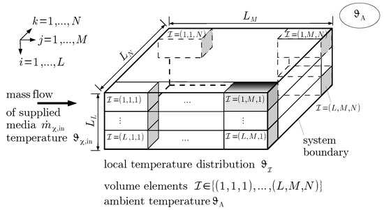
Figure 1. Spatial semi-discretization of the fuel cell stack module (arrangement of finitely large volume elements in up to three space coordinates) [16].

Table 1. Variables of the solid oxide fuel cell (SOFC) model.

Variable	Physical Meaning
${\vartheta }_{(1,1,1)}$, ${\vartheta }_{(1,2,1)}$, ${\vartheta }_{(1,3,1)}$	stack segment temperatures, discretization in the direction of gas mass flow
I	electric stack current
U	electric stack voltage
$\dot{U}$	temporal derivative of the electric stack voltage
$P_{\mathrm{EL}}$	electric power
${\dot{m}}_{\mathrm{CG}}$	mass flow of supplied cathode gas (preheated air)
${\vartheta }_{\mathrm{CG},\mathrm{m}}$	gas inlet temperature at the cathode
${\dot{m}}_{{\mathrm{N}}_2}$	nitrogen mass flow (anode)
${\dot{m}}_{{\mathrm{H}}_2}$	hydrogen mass flow (anode)
${\vartheta }_{\mathrm{AG},\mathrm{m}}$	gas inlet temperature at the anode
${\vartheta }_{\mathrm{A}}$	ambient temperature
subscript index $\mathrm{m}$	measured variable (added for distinction from simulation and estimation results)
subscript index k	discrete time index (sampling time: $0.1\mathrm{s}$)

2.1. Static Neural Network Model

As the fundamental, static electric power model, the neural network representation according to Figure 2 is considered. Its optimal configuration of inputs $q_j$, $j\in \{1,\dots ,m\}$, can be identified by the procedure summarized in Section 2.2.1. This procedure relies on a principal component analysis that is based on a singular value decomposition approach [34]. In [33], it was shown that the most relevant input parameters, which were acquired in [13,33] with a sampling frequency of $10\mathrm{Hz}$ at a test rig available at the University of Rostock, Germany, are given by the quantities marked with the ✔ symbols in the first row of Table 2.

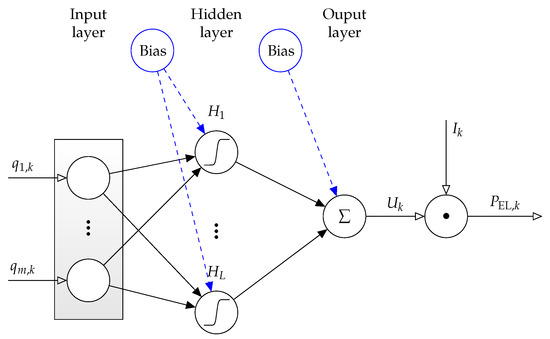
Figure 2. Static neural network model for the electric power characteristic of the SOFC stack with the network inputs ${\vartheta }_{\mathrm{m},(1,1,1),k}$, ${\vartheta }_{\mathrm{m},(1,3,1),k}$, $I_k$, ${\vartheta }_{\mathrm{CG},\mathrm{m},k}$, ${\dot{m}}_{{\mathrm{N}}_2,k}$, ${\dot{m}}_{{\mathrm{H}}_2,k}$, ${\vartheta }_{\mathrm{AG},\mathrm{m},k}$ and the output $U_k$.

Table 2. Optimal network input selection for the neural network representations of the electric power characteristic according to Figure 2 (first row) and Figure 5 (second row), where ${\dot{m}}_{{\mathrm{N}}_2}\approx 5.1·{10}^{-4}\frac{\mathrm{kg}}{\mathrm{s}}=\mathrm{const}$. The indices $\mathrm{AG}$ and $\mathrm{CG}$ denote the anode and cathode gas components, respectively, while ${\vartheta }_{\mathrm{A}}$ is the ambient temperature.

Network Type	Network Inputs ${\mathbf{q}}_{\mathit{k}}$
	${\vartheta }_{(1,1,1)}$	${\vartheta }_{(1,2,1)}$	${\vartheta }_{(1,3,1)}$	I	U	${\dot{m}}_{\mathrm{CG}}$	${\vartheta }_{\mathrm{CG},\mathrm{m}}$	${\dot{m}}_{{\mathrm{N}}_2}$	${\dot{m}}_{{\mathrm{H}}_2}$	${\vartheta }_{\mathrm{AG},\mathrm{m}}$	${\vartheta }_{\mathrm{A}}$
static voltage prediction (Figure 2, Figure 7 and Figure 9)	✔	✘	✔	✔	✘	✘	✔	✔	✔	✔	✘
dynamic voltage prediction (Figure 5)	✔	✘	✔	✔	✔	✘	✔	✔	✔	✔	✘

According to Figure 2, the neural network (where the number of hidden layer neurons with hyperbolic tangent activation functions was reduced from an initially overparameterized model with $L=30$ to $L=7$, by using the principal component analysis from Section 2.2.2) produces the stack voltage $U_k$, sampled at the same time instants k for which the vector ${\mathbf{q}}_k$ of input data is given. A multiplication of the network output with the terminal current $I_k$ of the SOFC stack then provides the corresponding power $P_{\mathrm{EL},k}$. If the layer weights and bias variables which are highlighted by the filled arrow heads in Figure 2 are optimized in Matlab by means of the standard Bayesian regularization back-propagation algorithm (parallelized on four CPU cores) with a maximum number of 5000 epochs, in which a worsening of the validation performance was allowed in 50 subsequent iterations, the model accuracy according to Figure 3 is obtained. From the depicted horizon of data, a random subdivision into training (70%), test (15%), and validation (15%) data was performed as described in [33]. Note, the data in the current paper does not only contain the measurements from [33] (the first approx. 1.5 hours of the depicted values in Figure 3) but further experiments in which the hydrogen mass flow was adapted for a constant electric current with variable power. These data were acquired in the experiments published in [13].

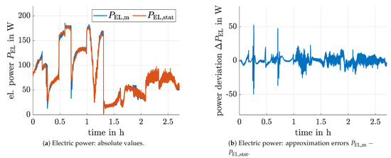
Figure 3. Comparison between measured and estimated stack power, $P_{\mathrm{EL},\mathrm{m}}$ and $P_{\mathrm{EL},\mathrm{stat}}$, for the system model in Figure 2.

To show the variability of the SOFC input parameters $q_{j,k}$, their respective measurements are summarized in Figure 4. These further system inputs are identical for the alternative, dynamic representations for the electric power characteristics described in the Section 2.3, Section 2.4 and Section 2.5.

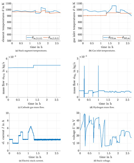
Figure 4. System inputs for the neural network model identification (experimental data).

2.2. Optimization of the Neural Network Structure

In this subsection, a brief overview of the singular value decomposition approach for finding optimal neural network inputs as well as for the optimization of the numbers of hidden layer neurons is given. For implementation details, the reader is referred to [33].

2.2.1. Optimal Network Inputs

The selection of optimal (non-redundant and sufficiently information carrying) network inputs is performed by means of a subset selection that is based on a singular value decomposition of suitable matrices [34]. To find the optimal network inputs, the training data matrix $\mathbf{T}\in {\mathbb{R}}^{l\times m}$ is considered, where l denotes the number of training samples; m is the number of inputs to the networks, cf. Figure 2. Using this matrix $\mathbf{T}$, a singular value decomposition is performed according to

$$\mathbf{T}={\mathbf{U}}_{\mathrm{T}}{\Sigma }_{\mathrm{T}}{\mathbf{V}}_{\mathrm{T}}^T,$$

(1)

where ${\mathbf{U}}_{\mathrm{T}}^T{\mathbf{U}}_{\mathrm{T}}=\mathbf{I}$ and ${\mathbf{V}}_{\mathrm{T}}^T{\mathbf{V}}_{\mathrm{T}}=\mathbf{I}$ with the identity matrix $\mathbf{I}\in {\mathbb{R}}^{m\times m}$ hold. Due to the fact that the number of training samples exceeds the number of network inputs, $l>m$ holds. Then, ${\Sigma }_{\mathrm{T}}$ is a block matrix

$${\Sigma }_{\mathrm{T}}=\left[\begin{array}{c}\mathrm{diag}\{{\sigma }_{\mathrm{T},1},\dots ,{\sigma }_{\mathrm{T},m}\}\\ {\mathbf{0}}_{(l-m)\times m}\end{array}\right],$$

(2)

where ${\sigma }_{\mathrm{T},1}\ge {\sigma }_{\mathrm{T},2}\ge \dots \ge {\sigma }_{\mathrm{T},m}\ge 0$ are the singular values sorted in descending order and ${\mathbf{0}}_{(l-m)\times m}\in {\mathbb{R}}^{(l-m)\times m}$ is a zero matrix of appropriate dimension.

The number ${\eta }_{\mathrm{T}}>1$ of relevant system inputs is identified as the largest integer for which

$$\sum _{i=1}^{{\eta }_{\mathrm{T}}}{\sigma }_{\mathrm{T},i}^{\prime }\le 1-{ϵ}_{\mathrm{T}}$$

(3)

holds with the normalized singular values

$${\sigma }_{\mathrm{T},i}^{\prime }={\sigma }_{\mathrm{T},i}·{\left(\sum _{i=1}^m{\sigma }_{\mathrm{T},i}\right)}^{-1}$$

(4)

and the sufficiently small threshold value $0<{ϵ}_{\mathrm{T}}\ll 1$.

According to [34], define the matrix ${\overline{\mathbf{V}}}_{\mathrm{T}}$ as the first ${\eta }_{\mathrm{T}}$ columns of ${\mathbf{V}}_{\mathrm{T}}$ and partition it into

$${\overline{\mathbf{V}}}_{\mathrm{T}}=\left[\begin{array}{cc}{\overline{\mathbf{V}}}_{\mathrm{T},1}& {\overline{\mathbf{V}}}_{\mathrm{T},2}\end{array}\right]$$

(5)

with ${\overline{\mathbf{V}}}_{\mathrm{T},1}\in {\mathbb{R}}^{{\eta }_{\mathrm{T}}\times {\eta }_{\mathrm{T}}}$ and ${\overline{\mathbf{V}}}_{\mathrm{T},2}\in {\mathbb{R}}^{(m-\eta )\times {\eta }_{\mathrm{T}}}$. Performing a QR factorization of ${\overline{\mathbf{V}}}_{\mathrm{T}}^T$ with column pivoting yields a permutation matrix ${\mathbf{P}}_{\mathrm{T}}\in {\mathbb{R}}^{m\times m}$ such that

$${\mathbf{Q}}^T{\left[\begin{array}{cc}{\overline{\mathbf{V}}}_{\mathrm{T},1}& {\overline{\mathbf{V}}}_{\mathrm{T},2}\end{array}\right]}^T{\mathbf{P}}_{\mathrm{T}}=\left[\begin{array}{cc}{\mathbf{R}}_{\mathrm{T},1}& {\mathbf{R}}_{\mathrm{T},2}\end{array}\right]$$

(6)

holds so that ${\mathbf{R}}_{\mathrm{T},1}$ is upper triangular and ${\mathbf{Q}}_{\mathrm{T}}^T{\mathbf{Q}}_{\mathrm{T}}=\mathbf{I}$. Now, the selected input subset ${\mathbf{T}}_1$ is obtained as

$$\mathbf{T}{\mathbf{P}}_{\mathrm{T}}\equiv \left[\begin{array}{cc}{\mathbf{T}}_1& {\mathbf{T}}_2\end{array}\right],$$

(7)

where ${\mathbf{T}}_1\in {\mathbb{R}}^{l\times {\eta }_{\mathrm{T}}}$. For consistency with Figure 2, the number ${\eta }_{\mathrm{T}}$ is afterwards renamed into m.

2.2.2. Optimal Number of Hidden Layer Neurons

The selection of an optimal number of hidden neurons basically follows the same procedure as described for the optimal input selection. The major difference is that the matrix $\mathbf{T}$ from the previous subsection is now replaced by a matrix $\mathbf{H}\in {\mathbb{R}}^{l\times L}$, where L is the number of neurons in the hidden layer. This matrix is determined from a simulation of an over-parameterized neural network after its training up to the point of reasonable convergence. Then, the matrix $\mathbf{H}$ is used to determine the singular value decomposition ${\mathbf{U}}_{\mathrm{H}}$, ${\Sigma }_{\mathrm{H}}$, ${\mathbf{V}}_{\mathrm{H}}$, from which the $1\le {\eta }_{\mathrm{H}}<L$ most important singular values are extracted after specifying a small positive threshold ${ϵ}_{\mathrm{H}}$. This number ${\eta }_{\mathrm{H}}$ characterizes a systematically chosen number of hidden layer neurons with which the training can be re-initialized. In general, further reductions may be possible by executing the singular value decomposition again after completion of the training phase, cf. [33].

2.3. First-Order Dynamic Neural Network Model

An extension of the static neural network system model described in the Section 2.1 is given in Figure 5. It is obtained by training the relationship between the input vector ${\mathbf{q}}_k$ (second row of Table 2) which has been augmented by the stack voltage $U_k$ as a further input variable. In this model, the time derivative ${\dot{U}}_k$ is treated as the neural network output. As described in detail in [33], the inputs and the output of this neural network need to be low-pass filtered with identical time constants so that no undesired phase shifts occur. Moreover, the variable ${\dot{U}}_k$ is obtained—for the network’s training phase—by a numerical derivative approximation after the aforementioned filtering.

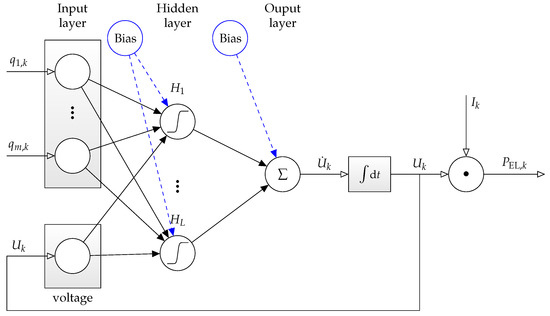
Figure 5. Dynamic neural network model for the electric power characteristic of the SOFC stack with the network inputs ${\vartheta }_{\mathrm{m},(1,1,1),k}$, ${\vartheta }_{\mathrm{m},(1,3,1),k}$, $I_k$, ${\vartheta }_{\mathrm{CG},\mathrm{m},k}$, ${\dot{m}}_{{\mathrm{N}}_2,k}$, ${\dot{m}}_{{\mathrm{H}}_2,k}$, ${\vartheta }_{\mathrm{AG},\mathrm{m},k}$, $U_k$ and the output ${\dot{U}}_k$.

For the application of this neural network, the time derivative ${\dot{U}}_k$ of the stack voltage is numerically integrated and fed back to the network’s input layer. Moreover, the electric power is obtained in analogy to the previous system model by a multiplication of $U_k$, i.e., the integrator output, with the electric current $I_k$. As in Section 2.1, the training has been started with an over-parameterized hidden layer containing $L=30$ neurons. Their number was reduced by means of the principal component analysis summarized in Section 2.2.2 to $L=9$. A comparison of the root mean square approximation error of this network in Table 4 with the static alternative from Figure 2 shows a slightly worse approximation of the actual fuel cell power. Hence, this option (visualized in Figure 6) is not considered for the numerical validation of the proposed filter-based estimation and optimization procedure of this paper. Instead, the dynamic system models described in the following two subsections are employed.

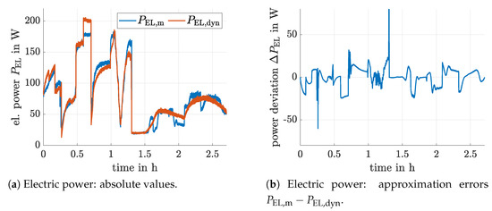
Figure 6. Comparison between measured and estimated stack power, $P_{\mathrm{EL},\mathrm{m}}$ and $P_{\mathrm{EL},\mathrm{dyn}}$, for the system model in Figure 5.

2.4. Hammerstein Neural Network Model with Integer-Order Dynamics

Hammerstein models are generally composed of a static input nonlinearity which forms the input to a linear dynamic system. Following this philosophy, the system model in Figure 7 is obtained. Here, the input nonlinearity is given by the same neural network already described in Section 2.1. Due to the fact that the linear transfer function $G_{\mathrm{IO}}\left(s\right)$ in Figure 7 is a pure linear low-pass filter with gain equal to one, the steady-state outputs of both the neural network and the linear transfer function, i.e., ${\tilde{U}}_k$ and $U_k$, respectively, are identical.

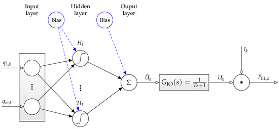
Figure 7. Hammerstein-type dynamic model for the electric power characteristic of the SOFC stack with integer-order dynamics with the network inputs ${\vartheta }_{\mathrm{m},(1,1,1),k}$, ${\vartheta }_{\mathrm{m},(1,3,1),k}$, $I_k$, ${\vartheta }_{\mathrm{CG},\mathrm{m},k}$, ${\dot{m}}_{{\mathrm{N}}_2,k}$, ${\dot{m}}_{{\mathrm{H}}_2,k}$, ${\vartheta }_{\mathrm{AG},\mathrm{m},k}$ and the output ${\tilde{U}}_k$.

Hence, this Hammerstein-type extension of the static neural network model in Figure 2 aims at describing the transient processes for rapid changes in the inputs ${\mathbf{q}}_k$ with enhanced accuracy. As before, the electric power $P_{\mathrm{EL},k}$ is obtained by a pure multiplication of $U_k$ with $I_k$. Note, due to the restriction of $G_{\mathrm{IO}}\left(s\right)$ to a first-order transfer function, the only parameter to be optimized in this system model is the time constant $T>0\mathrm{s}$. This parameter is obtained by numerically solving a least squares optimization problem in which the integral over the squared difference between the measured and simulated stack voltages $U_k$ is minimized. If the simulation step size is set equal to the sampling step size at which measured data are available ($100\mathrm{ms}$), the lower parameter bound $T\ge 0.5\mathrm{s}$ ensures that the discretization of the transfer function $G_{\mathrm{IO}}\left(s\right)$ by means of an explicit Euler method is sufficiently accurate.

A further increase of the order of the transfer function $G_{\mathrm{IO}}\left(s\right)$ did not show any significant improvement of the model accuracy. Therefore, only this first-order model is visualized in Figure 8 and listed in Table 4.

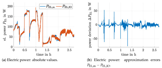
Figure 8. Comparison between measured and estimated stack power, $P_{\mathrm{EL},\mathrm{m}}$ and $P_{\mathrm{EL},\mathrm{IO}}$, for the system model in Figure 7.

2.5. Hammerstein Neural Network Model with Fractional-Order Dynamics

The fractional-order extension in Figure 9 follows the same principal idea as the use of the integer-order filter in the previous subsection. The only change is the replacement of the integer-order powers of the Laplace variable s in the transfer function $G_{\mathrm{IO}}\left(s\right)$ by non-integer values in $G_{\mathrm{FO}}\left(s\right)$. In the time domain, this corresponds to a fractional derivative order $\nu$ with $0<\nu \le 1$. Note, for $\nu \equiv 1$ with $n=1$, this model becomes equal to the one of Section 2.4. However, for $\nu \ne 1$, it provides a further degree of freedom for the optimization in addition to the numerator and denominator coefficients $b_i$ and $a_i$.

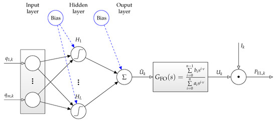
Figure 9. Hammerstein-type dynamic model for the electric power characteristic of the SOFC stack with fractional-order dynamics with the network inputs ${\vartheta }_{\mathrm{m},(1,1,1),k}$, ${\vartheta }_{\mathrm{m},(1,3,1),k}$, $I_k$, ${\vartheta }_{\mathrm{CG},\mathrm{m},k}$, ${\dot{m}}_{{\mathrm{N}}_2,k}$, ${\dot{m}}_{{\mathrm{H}}_2,k}$, ${\vartheta }_{\mathrm{AG},\mathrm{m},k}$ and the output ${\tilde{U}}_k$.

A numerical optimization in the least-squares sense for the choice of $n=1$ and $n=3$ led to the parameter values listed in Table 3. The resulting root of the mean square approximation error (RMS) and the corresponding graphical comparison of both models can be found in Table 4 as well as in Figure 10a–d.

Table 3. Parameters for the fractional-order transfer function $G_{\mathrm{FO}}\left(s\right)$ in Figure 2 and Figure 5 on the basis of the optimized neural network with $L=7$ hidden neurons (the fact that $\frac{b_0}{a_0}\ne 1$ indicates a static gain adaptation by the employed optimization routine).

Order n	Order $\mathit{\nu }$	${\mathit{a}}_0$	${\mathit{a}}_1$	${\mathit{a}}_2$	${\mathit{a}}_3$	${\mathit{b}}_0$	${\mathit{b}}_1$	${\mathit{b}}_2$
1	$0.4864$	$2.5784$	$1.0000$	−	−	$2.5951$	−	−
3	$0.7195$	$0.5000$	$0.6053$	$6.4360$	$1.0000$	$0.5013$	$5.43·{10}^{-5}$	$6.8654$

Table 4. Overview of the training and simulation results for the neural network models in Figure 2, Figure 5, Figure 7 and Figure 9.

No.	Network Type	Optimized?	Training Data					Hidden Neurons	RMS
			${\dot{\vartheta }}_{(1,1,1)}$	${\dot{\vartheta }}_{(1,2,1)}$	${\dot{\vartheta }}_{(1,3,1)}$	$\dot{U}$	U
Figure 2	voltage prediction (static)	✘	✘	✘	✘	✘	✔	30	$7.1388\mathrm{W}$
Figure 2	voltage prediction (static)	✔	✘	✘	✘	✘	✔	7	$5.5677\mathrm{W}$
Figure 5	voltage prediction (dynamic)	✘	✘	✘	✘	✔	✘	30	$10.5563\mathrm{W}$
Figure 5	voltage prediction (dynamic)	✔	✘	✘	✘	✔	✘	9	$10.8218\mathrm{W}$
Figure 7	voltage prediction ($G_{\mathrm{IO}}\left(s\right)$)	✘	✘	✘	✘	✘	✔	30	$7.1413\mathrm{W}$
Figure 7	voltage prediction ($G_{\mathrm{IO}}\left(s\right)$)	✔	✘	✘	✘	✘	✔	7	$5.4972\mathrm{W}$
Figure 9	voltage prediction ($G_{\mathrm{FO}}\left(s\right)$, $n=1$)	✘	✘	✘	✘	✘	✔	30	$7.1469\mathrm{W}$
Figure 9	voltage prediction ($G_{\mathrm{FO}}\left(s\right)$, $n=1$)	✔	✘	✘	✘	✘	✔	7	$5.3782\mathrm{W}$
Figure 9	voltage prediction ($G_{\mathrm{FO}}\left(s\right)$, $n=3$)	✘	✘	✘	✘	✘	✔	30	$7.1726\mathrm{W}$
Figure 9	voltage prediction ($G_{\mathrm{FO}}\left(s\right)$, $n=3$)	✔	✘	✘	✘	✘	✔	7	$5.3876\mathrm{W}$

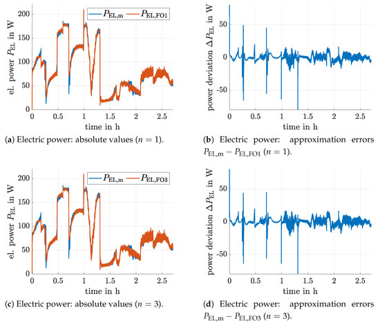
Figure 10. Comparison between measured and estimated stack power, $P_{\mathrm{EL},\mathrm{m}}$ and $P_{\mathrm{EL},\mathrm{FO}1}$ (resp., $P_{\mathrm{EL},\mathrm{FO}3}$), for the system model in Figure 9.

For the numerical evaluation of the fractional differential equations, which represent the time domain formulation

$$\sum _{i=0}^n{a}_i·\frac{{\mathrm{d}}^{(i·\nu )}U\left(t\right)}{\mathrm{d}{t}^{(i·\nu )}}=\sum _{i=0}^{n-1}{b}_i·\frac{{\mathrm{d}}^{(i·\nu )}\tilde{U}\left(t\right)}{\mathrm{d}{t}^{(i·\nu )}}$$

(8)

of the transfer function $G_{\mathrm{FO}}\left(s\right)$, the Matlab solver fde12 published in [35] was employed.

Due to the fact that the change of the model accuracy between $n=1$ and $n=3$ is negligibly small, the further numerical evaluations are based on the system models from Figure 2, Figure 7 and Figure 9, where $n=3$ is chosen for the fractional-order system representation.

3. Kalman Filter-Based Power Estimation and Online Parameter Identification

To implement an instationary Kalman filter [26,27,28] on the basis of a general discrete-time system model

$${\mathbf{x}}_{k+1}={\mathbf{A}}_k{\mathbf{x}}_k+{\mathbf{E}}_k{\mathbf{w}}_k$$

(9)

with the measurement equation

$${\mathbf{y}}_k={\mathbf{C}}_k{\mathbf{x}}_k+{\mathbf{v}}_k,$$

(10)

the electric power characteristic of the SOFC is locally approximated at each time instant k by a polynomial in the electric current and the hydrogen mass flow according to

$$P_{\mathrm{EL},k}\approx \left({\mathbf{I}}_k^{\left[m_1-1\right]}\otimes {\dot{\mathbf{m}}}_{{\mathrm{H}}_2,k}^{\left[m_2-1\right]}\right)·{\mathbf{x}}_k.$$

(11)

Here, the coefficient vector ${\mathbf{x}}_k\in {\mathbb{R}}^{{\prod }_{i=1}^2{m}_i}$ represents the state vector to be estimated by the Kalman filter. In addition, the Kronecker product which connects the vectors of monomials of both the current and the hydrogen mass flow is denoted by ⊗.

Setting $m_1=m_2=3$ in

$${\mathbf{I}}_k^{\left[m_1-1\right]}=\left[\begin{array}{ccccc}{I}_k^0& I_k^1& I_k^2& \dots & I_k^{m_1-1}\end{array}\right]$$

(12)

as well as

$${\dot{\mathbf{m}}}_{{\mathrm{H}}_2,k}^{\left[m_2-1\right]}=\left[\begin{array}{ccccc}{\dot{m}}_{{\mathrm{H}}_2,k}^0& {\dot{m}}_{{\mathrm{H}}_2,k}^1& {\dot{m}}_{{\mathrm{H}}_2,k}^2& \dots & {\dot{m}}_{{\mathrm{H}}_2,k}^{m_2-1}\end{array}\right],$$

(13)

second-order polynomials are obtained in both the electric current and the hydrogen mass flow. This system model is a generalization of the one used in [25] (Equation (12)), where only electric current dependencies were accounted for.

As mentioned above, the vector ${\mathbf{x}}_k$ of yet unknown coefficients is treated as the state vector of the Kalman filter. Its entries need to be adjusted at run-time to account for the influence of changes of the stack temperature, the gas inlet temperatures and the cathode gas and nitrogen mass flows. This adjustment is made on the basis of the voltage and current measurements $U_k$ and $I_k$, respectively. Thus, the measured power $P_{\mathrm{EL},k}=U_k·I_k$ serves as a scalar realization of the general output vector ${\mathbf{y}}_k$ given in Equation (10).

In general, the Kalman filter for the system model (9) with (10) consists of the prediction step

$$\begin{array}{cc}\hfill {\mathit{\mu }}_{x,k+1}^{\mathrm{p}}& ={\mathbf{A}}_k{\mathit{\mu }}_{x,k}^{\mathrm{e}}+{\mathbf{E}}_k{\mathit{\mu }}_{w,k}\hfill \end{array}$$

(14)

$$\begin{array}{cc}\hfill {\mathbf{C}}_{x,k+1}^{\mathrm{p}}& ={\mathbf{A}}_k{\mathbf{C}}_{x,k}^{\mathrm{e}}{\mathbf{A}}_k^T+{\mathbf{E}}_k{\mathbf{C}}_{w,k}{\mathbf{E}}_k^T\hfill \end{array}$$

(15)

as well as the measurement-based innovation

$$\begin{array}{cc}\hfill {\mathit{\mu }}_{x,k}^{\mathrm{e}}& ={\mathit{\mu }}_{x,k}^{\mathrm{p}}+{\mathbf{L}}_k·\left({\widehat{\mathbf{y}}}_k-{\mathbf{C}}_k{\mathit{\mu }}_{x,k}^{\mathrm{p}}-{\mathit{\mu }}_{v,k}\right)\hfill \end{array}$$

(16)

$$\begin{array}{cc}\hfill {\mathbf{C}}_{x,k}^{\mathrm{e}}& ={\mathbf{C}}_{x,k}^{\mathrm{p}}-{\mathbf{L}}_k{\mathbf{C}}_k{\mathbf{C}}_{x,k}^{\mathrm{p}}\hfill \end{array}$$

(17)

with the time-varying Kalman gain

$${\mathbf{L}}_k={\mathbf{C}}_{x,k}^{\mathrm{p}}{\mathbf{C}}_k^T{\left({\mathbf{C}}_k{\mathbf{C}}_{x,k}^{\mathrm{p}}{\mathbf{C}}_k^T+{\mathbf{C}}_{v,k}\right)}^{-1}.$$

(18)

Here, in full analogy to [25], the noise processes ${\mathbf{w}}_k$ and ${\mathbf{v}}_k$ are assumed to be given by the stochastically independent normal distributions $\mathcal{N}\left(\mathit{\xi },{\mathit{\mu }}_{\xi },{\mathbf{C}}_{\xi }\right)$, $\mathit{\xi }\in \left\{{\mathbf{w}}_k,{\mathbf{v}}_k\right\}$, $\mathit{\xi }\in {\mathbb{R}}^{n_{\xi }}$ with

$$\mathcal{N}\left(\mathit{\xi },{\mathit{\mu }}_{\xi },{\mathbf{C}}_{\xi }\right)=\frac{1}{\sqrt{{\left(2\pi \right)}^{n_{\xi }}·det\left({\mathbf{C}}_{\xi }\right)}}·exp\left(-\frac{1}{2}{(\mathit{\xi }-{\mathit{\mu }}_{\xi })}^T{\mathbf{C}}_{\xi }^{-1}(\mathit{\xi }-{\mathit{\mu }}_{\xi })\right)$$

(19)

and the corresponding mean vectors ${\mathit{\mu }}_{\xi }$ and covariance matrices ${\mathbf{C}}_{\xi }$. Under the assumption that both process and measurement noise have a vanishing mean, ${\mathit{\mu }}_{\xi }\equiv \mathbf{0}$ holds.

Due to the fact that the vector ${\mathbf{x}}_k$ describes slow variations of the parameters of the electric power characteristic of the SOFC in a model-free way, the system matrix ${\mathbf{A}}_k$ in (9) is set to the identity matrix ${\mathbf{I}}_{9\times 9}\in {\mathbb{R}}^{9\times 9}$. This corresponds to representing the dynamics of these parameters by a so-called discrete-time integrator disturbance model, see also [25].

Due to the assumption of independent Gaussian noise processes for all components of the state vector, the disturbance input matrix simplifies to ${\mathbf{E}}_k={\mathbf{I}}_{9\times 9}$ with a purely diagonal covariance matrix ${\mathbf{C}}_{w,k}=\mathrm{diag}\left\{\left[\begin{array}{ccc}{\sigma }_{w,1}^2& \dots & {\sigma }_{w,9}^2\end{array}\right]\right\}$. It is parameterized by means of the standard deviations ${\sigma }_{w,i}$, $i\in \{1,\dots ,9\}$, of the state variabilities between two subsequent sampling steps. These entries can be used as tuning factors in the Kalman filter parameterization to ensure a sufficiently fast convergence of the local approximation to the true electric power characteristic.

With the help of this model, the predicted parameters (superscript $\mathrm{p}$) of the electric power characteristic can be described by the vector $\mathrm{E}\left\{{\mathbf{x}}_{k+1}\right\}={\mathit{\mu }}_{x,k+1}^{\mathrm{p}}$ of expected values together with the corresponding covariance matrix ${\mathbf{C}}_{x,k+1}^{\mathrm{p}}$ according to

$$\begin{array}{cc}\hfill {\mathit{\mu }}_{x,k+1}^{\mathrm{p}}& ={\mathit{\mu }}_{x,k}^{\mathrm{e}}\mathrm{and}\hfill \end{array}$$

(20)

$$\begin{array}{cc}\hfill {\mathbf{C}}_{x,k+1}^{\mathrm{p}}& ={\mathbf{C}}_{x,k}^{\mathrm{e}}+{\mathbf{C}}_{w,k}.\hfill \end{array}$$

(21)

Here, the superscript symbol $\mathrm{e}$ on the right-hand sides denotes the outcome of the previous innovation step. For the scalar power measurement (11) with the variance $C_{v,k}$, the innovation step at the time instant k—which precedes the prediction (20), (21)—is given by

$$\begin{array}{cc}\hfill {\mathit{\mu }}_{x,k}^{\mathrm{e}}& ={\mathit{\mu }}_{x,k}^{\mathrm{p}}+{\mathbf{L}}_k·\left({\widehat{y}}_k-{\overline{\mathbf{y}}}_k^T·{\mathit{\mu }}_{x,k}^{\mathrm{p}}\right)\mathrm{and}\hfill \end{array}$$

(22)

$$\begin{array}{cc}\hfill {\mathbf{C}}_{x,k}^{\mathrm{e}}& ={\mathbf{C}}_{x,k}^{\mathrm{p}}-{\mathbf{L}}_k·{\overline{\mathbf{y}}}_k^T·{\mathbf{C}}_{x,k}^{\mathrm{p}}.\hfill \end{array}$$

(23)

In (22) and (23), the time-varying Kalman gain introduced in (18) results in

$${\mathbf{L}}_k={\mathbf{C}}_{x,k}^{\mathrm{p}}·{\overline{\mathbf{y}}}_k·{\left({\overline{\mathbf{y}}}_k^T·{\mathbf{C}}_{x,k}^{\mathrm{p}}·{\overline{\mathbf{y}}}_k+C_{v,k}\right)}^{-1}\in {\mathbb{R}}^9,$$

(24)

where

$${\overline{\mathbf{y}}}_k^T=\left({\mathbf{I}}_k^{\left[2\right]}\otimes {\dot{\mathbf{m}}}_{{\mathrm{H}}_2,k}^{\left[2\right]}\right).$$

(25)

In [25], the standard deviation

$${\sigma }_{P_{\mathrm{EL}},k}=\sqrt{\mathrm{E}\left\{{\left(P_{\mathrm{EL},k}-\mathrm{E}\left\{P_{\mathrm{EL},k}\right\}\right)}^2\right\}}$$

(26)

was introduced for a quantification of the uncertainty in the approximation of the electric power characteristic. If both current and mass flow dependencies are accounted for, Equation (26) turns into

$$\begin{array}{cc}\hfill {\sigma }_{P_{\mathrm{EL}},k}& =\sqrt{\mathrm{E}\left\{{\overline{\mathbf{y}}}_k^T·\left({\mathbf{x}}_k-{\mathit{\mu }}_{x,k}^{\mathrm{e}}\right)·{\left({\mathbf{x}}_k-{\mathit{\mu }}_{x,k}^{\mathrm{e}}\right)}^T·{\overline{\mathbf{y}}}_k\right\}}\hfill \\ \hfill & =\sqrt{{\overline{\mathbf{y}}}_k^T·\mathrm{E}\left\{\left({\mathbf{x}}_k-{\mathit{\mu }}_{x,k}^{\mathrm{e}}\right)·{\left({\mathbf{x}}_k-{\mathit{\mu }}_{x,k}^{\mathrm{e}}\right)}^T\right\}·{\overline{\mathbf{y}}}_k}\hfill \\ \hfill & =\sqrt{{\overline{\mathbf{y}}}_k^T·{\mathbf{C}}_{x,k}^{\mathrm{e}}·{\overline{\mathbf{y}}}_k}.\hfill \end{array}$$

(27)

As soon as ${\sigma }_{P_{\mathrm{EL}},k}$ becomes approximately constant after a certain number of successive prediction and innovation steps, or falls below a certain threshold, adjustments of the stack current as well as the gas mass flow are admissible by the optimization procedure described in the following section. This criterion allows for a clear separation of the time scales of the transient phase of the Kalman filter-based parameter identification as well as of the following optimization procedure so that instabilities due to overlapping time scales are avoided. Moreover, ${\sigma }_{P_{\mathrm{EL}},k}$ serves as a quality criterion that allows for checking how close the actual operating state of the SOFC can come to a desired electric operating point.

Note, the goal of operating the SOFC in the region of Ohmic polarization is ensured if

$$\frac{\partial P_{\mathrm{EL},k}}{\partial I_k}\approx \left(\left[\begin{array}{ccccc}0& 1& 2I_k& \dots & \left(m_1-1\right)·I_k^{m_1-2}\end{array}\right]\otimes {\dot{\mathbf{m}}}_{{\mathrm{H}}_2,k}^{\left[m_2-1\right]}\right)·{\mathit{\mu }}_{x,k}^{\mathrm{e}}>0$$

(28)

holds.

4. Online Optimization of the Electric Current and Hydrogen Mass Flow

In this section, an online optimization of the electric current and hydrogen mass flow of the SOFC is implemented such that a desired operating point (specified by its desired electric power $P_{\mathrm{EL},\mathrm{d}}$) is attained. Simultaneously, the supplied hydrogen mass flow should be minimized. This is expressed by the cost function

$$J_k={\left(P_{\mathrm{EL},k}-P_{\mathrm{EL},\mathrm{d}}\right)}^2+{\gamma }_1{\dot{m}}_{{\mathrm{H}}_2,k}^2+{\gamma }_{2}ln\left(\frac{I_{max,k}}{I_{max,k}-I_k}\right)$$

(29)

with the electric power $P_{\mathrm{EL},k}$ according to (11), which is evaluated for the results ${\mathit{\mu }}_{x,k}^{\mathrm{e}}$ of the Kalman filter’s innovation step. The cost function $J_k$ includes a strict barrier in terms of a logarithmic term that helps to make sure that the electric current $I_k$ does not exceed its admissible upper bound $I_{max}$ according to the inequality

$$I_k<I_{max,k}:=\frac{z·F}{M_{{\mathrm{H}}_2}·N_{\mathrm{c}}}·{\dot{m}}_{{\mathrm{H}}_2,k}.$$

(30)

This inequality results from Faraday’s law and can alternatively be formulated as a lower limit ${\dot{m}}_{{\mathrm{H}}_2,min,k}$ for the supplied hydrogen mass flow

$${\dot{m}}_{{\mathrm{H}}_2,k}>{\dot{m}}_{{\mathrm{H}}_2,min,k}=\frac{M_{{\mathrm{H}}_2}·N_{\mathrm{c}}}{z·F}·I_k.$$

(31)

Here, $z=4$ is the number of electrons involved in the reaction between hydrogen and oxygen, $F=9.6485·{10}^4\frac{\mathrm{As}}{\mathrm{mol}}$ is Faraday’s constant, $M_{{\mathrm{H}}_2}=2.01588·{10}^{-3}\frac{\mathrm{kg}}{\mathrm{mol}}$ the molar mass of hydrogen, and $N_{\mathrm{c}}$ the number of (planar) fuel cells that are electrically connected in series under the assumption of a homogeneous mass flow over all of the cells. For compatibility with the system identification in Section 2, $N_{\mathrm{c}}=60$ is used in the following.

For both formulations (30) and (31), the boundary of the admissible operating domain is represented by an infinitely large cost in (29). This infinite cost is attained on the boundary of the admissible operating domain, i.e., for those conditions at which the hydrogen mass flow is completely consumed by the production of the actual electric power $P_{\mathrm{EL},k}$.

If the system’s optimization is initialized with an admissible operating point $\left(I_k,{\dot{m}}_{{\mathrm{H}}_2,k}\right)$ satisfying the inequalities (30) and (31), it is guaranteed by the following optimization scheme that all subsequent operating points are also admissible.

From a system theoretic perspective, the inclusion of the inequality (30), or alternatively (31), in the cost function (29) by means of logarithmic terms is inspired by the so-called barrier Lyapunov function technique [17,18,36]. It represents a kind of repelling potential that forces the optimization results to stay within the admissible operating domain. In other control-oriented research activities such approaches are employed to prove stability of a closed-loop controller in the presence of hard one- or two-sided state and output as well as actuator constraints. For further details about real-time capable strategies for parameter adaption of nonlinear robust feedback controllers exploiting such barrier functions, the reader is referred to [17,18,37] as well as to [38]. The focus of the last reference is on using sensitivity-based feedforward and predictive control procedures to avoid exceeding state constraints instead of exploiting barrier function techniques.

The online optimization of the cost function (29) is performed by means of a gradient descent method [39,40] for an adaptation of the control inputs

$${\mathbf{u}}_k={\left[\begin{array}{cc}{I}_k& {\dot{m}}_{{\mathrm{H}}_2,k}\end{array}\right]}^T$$

(32)

according to the update rule

$${\mathbf{u}}_{k+1}={\mathbf{u}}_k-\alpha ·\nabla J_k·J_k$$

(33)

with the step size parameter $\alpha >0$. To ensure a fully deterministic behavior of the optimization algorithm, only a single update step according to (33) is performed at each discretization instant.

The step size parameter $\alpha$ in (33) is set to

$$\alpha ={10}^{-3}·\frac{1}{\sqrt{\nabla J_k^T·\nabla J_k}}$$

(34)

for the implementation in the following section, where $\nabla J_k$ is the gradient of the cost function $J_k$ (with $P_{\mathrm{EL},k}$ as the measured power and ${\widehat{P}}_{\mathrm{EL},k}$ the estimate of the Kalman filter provided after executing the innovation stage)

$$\nabla J_k=\left[\begin{array}{c}{\displaystyle \frac{\partial J_k}{\partial I_k}}\\ {\displaystyle \frac{\partial J_k}{\partial {\dot{m}}_{{\mathrm{H}}_2,k}}}\end{array}\right]=\left[\begin{array}{c}2·\left(P_{\mathrm{EL},k}-P_{\mathrm{EL},\mathrm{d}}\right)·{\displaystyle \frac{\partial {\widehat{P}}_{\mathrm{EL},k}}{\partial I_k}}+{\gamma }_2·{\displaystyle \frac{1}{I_{max}-I_k}}\\ 2·\left(P_{\mathrm{EL},k}-P_{\mathrm{EL},\mathrm{d}}\right)·{\displaystyle \frac{\partial {\widehat{P}}_{\mathrm{EL},k}}{\partial {\dot{m}}_{{\mathrm{H}}_2,k}}}+2{\gamma }_1{\dot{m}}_{{\mathrm{H}}_2,k}\end{array}\right],$$

(35)

where

$${\displaystyle \frac{\partial {\widehat{P}}_{\mathrm{EL},k}}{\partial I_k}}:=\left(\left[\begin{array}{ccccc}0& 1& 2I_k& \dots & \left(m_1-1\right)·I_k^{m_1-2}\end{array}\right]\otimes {\dot{\mathbf{m}}}_{{\mathrm{H}}_2,k}^{\left[m_2-1\right]}\right)·{\mathit{\mu }}_{x,k}^{\mathrm{e}}$$

(36)

and

$${\displaystyle \frac{\partial {\widehat{P}}_{\mathrm{EL},k}}{\partial {\dot{m}}_{{\mathrm{H}}_2,k}}}:=\left({\mathbf{I}}_k^{\left[m_1-1\right]}\otimes \left[\begin{array}{ccccc}0& 1& 2{\dot{m}}_{{\mathrm{H}}_2,k}& \dots & \left(m_2-1\right)·{\dot{m}}_{{\mathrm{H}}_2,k}^{m_2-2}\end{array}\right]\right)·{\mathit{\mu }}_{x,k}^{\mathrm{e}}$$

(37)

hold. Note, all current and mass flow dependencies of the expressions in (35)–(37) are expressed in terms of the previous commanded values ${\mathbf{u}}_k$, so that filtering of these quantities is not required for an online implementation.

As described in the previous section, updates of ${\mathbf{u}}_k$ are only executed when ${\sigma }_{P_{\mathrm{EL}},k}$ in (27) is approximately constant for at least $10\mathrm{s}$ or sufficiently small. If this is not the case, ${\mathbf{u}}_{k+1}={\mathbf{u}}_k$ is used in the following numerical validation.

Moreover, the further parameters used for the optimization in the following section are ${\gamma }_1=100$ and ${\gamma }_2=1$. Due to the relatively long time constants for variations of operating points in SOFCs, the optimization procedure is evaluated each second, i.e., at each tenth sampling point of the Kalman filter. It performs an underlying check whether the inequality (28) can be expected to be satisfied in the following time step. If not, the electric current is reduced. To avoid too large update steps by the previously introduced scaling factor $\alpha$, this value is reduced if the update leads to mass flow variations that exceed $1\%$ of the current amount of supplied hydrogen. Moreover, the hydrogen mass flow is kept constant if the gradient-based update rule suggests its reduction in cases when its current value is only $5\%$ larger than the limit given in (31). Then, only adaptations of $I_k$ are performed.

5. Numerical Validation

The numerical validation of the Kalman filter and its use for the online input optimization of the SOFC is subdivided into two subsections. First, the capability of detecting a system operation in the regime of Ohmic polarization, characterized by the increasing branch of the estimated power characteristic is demonstrated on the basis of the simulation models shown in Section 2. Second, the Kalman filter is initialized on the basis of these simulations up to a certain point of time, at which the online optimal control is activated.

5.1. Identification of Operation in Ohmic Polarization

In Figure 11, it is shown exemplarily for the static neural network model as well as for the proposed fractional-order system representation that the Kalman filter according to Section 3 can identify regions, where the operating point overshoots the point of maximum electric power. Note, all system inputs ${\mathbf{q}}_k$ of the evaluated models are given by the experimental data depicted in Section 2.

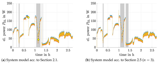
Figure 11. Detection of operating points exceeding the maximum power point.

Those regions, where the operating point exceeds the maximum power point, are visualized in gray color in Figure 11. Note, although different simulation approaches were employed in both subgraphs, the estimation results are in good coincidence. Orange color indicates the estimated expected value ${\widehat{P}}_{\mathrm{EL},k}$, while the two further colors represent the interval $\left[{\widehat{P}}_{\mathrm{EL},k}-3{\sigma }_{P_{\mathrm{EL}},k};{\widehat{P}}_{\mathrm{EL},k}+3{\sigma }_{P_{\mathrm{EL}},k}\right]$ in which the standard deviation ${\sigma }_{P_{\mathrm{EL}},k}$ is estimated according to (27).

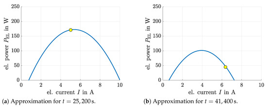
Figure 12 analyzes the previous statements concerning the overshoot detection with respect to the maximum power point in more detail. Setting the mass flow equal to the measured values at two selected points of time, see Figure 11a, the local quadratic approximations of the power characteristic can be depicted as function of the stack current. Obviously, Figure 12a represents an operating condition, where the system is close to its maximum power point, while in Figure 12b a reduction of the stack current (and/or, respectively, increase of the hydrogen mass flow) would be necessary to ensure the operation in the regime of Ohmic polarization.

Figure 12. Estimated quadratic approximations of the power characteristics as a function of the electric current I for operating points not exceeding the maximum power point (Figure 12a) and exceeding this critical point (Figure 12b).

5.2. Validation of the Kalman Filter-Based Input Optimization

Figure 13, Figure 14 and Figure 15 depict the optimization of the input vector ${\mathbf{u}}_k$ as described in Section 4. For the analysis of the robustness of the proposed optimization scheme, three different types of desired power variations are considered. These are

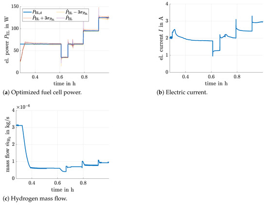
Figure 13. Input optimization for the fractional-order system model with $n=3$ for step-wise changes of the desired electric power.

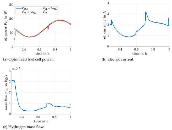
Figure 14. Input optimization for the integer-order system model for sinusoidal changes of the desired electric power.

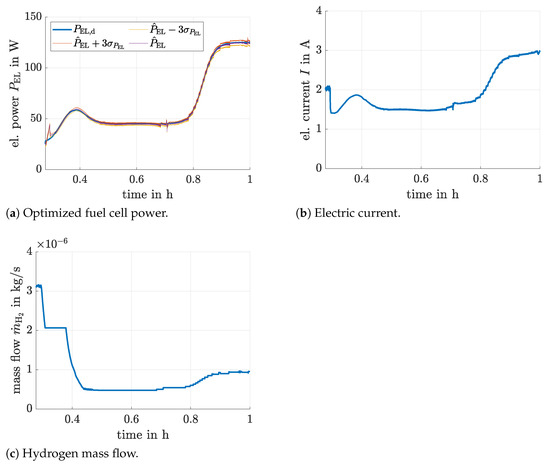
Figure 15. Input optimization for the static neural network system model with $n=3$ for smooth changes of the desired electric power.

• step-wise changes,
• sinusoidal power variations, and
• a smooth transition between operating points that is characterized by the superposition of $atanh$ functions.

In all three cases, the first $1000\mathrm{s}$ of the data from Section 2 were employed to initialize the Kalman filter (note, in practice, also much shorter phases are sufficient; the choice is only motivated by the fact that the adaptation of ${\mathbf{u}}_k$ should be restricted to a domain in which overshooting the maximum power point is avoided). All three depicted optimization results as well as the comparison of the roots of the mean square tracking error according to Table 5 show an excellent performance of the proposed methodology. A further smoothening of the input signals and a reduction of remaining tracking errors could be achieved by a combination with the closed-loop controllers presented in [13], for which the method presented in Section 4 could be used as a kind of feedforward control signal generator.

Table 5. Comparison of the tracking behavior of the proposed input optimization scheme for various system models and different types of reference signals for the desired electric power.

System Model	Reference Signal	RMS
Figure 2	step-wise changes	$5.3969\mathrm{W}$
Figure 2	sinusoidal	$4.8799\mathrm{W}$
Figure 2	smooth	$1.2417\mathrm{W}$
Figure 7	step-wise changes	$5.6445\mathrm{W}$
Figure 7	sinusoidal	$4.9088\mathrm{W}$
Figure 7	smooth	$2.1662\mathrm{W}$
Figure 9 ($n=3$)	step-wise changes	$5.3298\mathrm{W}$
Figure 9 ($n=3$)	sinusoidal	$4.7466\mathrm{W}$
Figure 9 ($n=3$)	smooth	$1.3455\mathrm{W}$

Finally, it should be pointed out that the proposed estimation and optimization procedure is readily implementable for real-time applications. This is underlined by the fact that the average computing times of the Kalman filter-based estimation in combination with the input optimization were approx. $22.3\mathsf{\mu }\mathrm{s}$ with a standard deviation of $54.9\mathsf{\mu }\mathrm{s}$ on a standard notebook computer under Windows 10, 64 bit, Intel i5-8365U CPU @1.60GHz, in a Matlab 2019b implementation in which no specific optimizations by means of precompiling individual subroutines were performed. Note, this computing time is smaller by more than a factor of 1000 than the sampling period so that it does not impose any severe restrictions concerning real-time implementability.

6. Conclusions and Outlook on Future Work

In this paper, a real-time implementable Kalman filter-based optimization procedure for tracking temporally varying electric power demands of SOFCs was presented. This approach allows for a robust optimization of the fuel utilization. It is readily applicable to real-life applications and computationally cheap to implement.

As it has been shown that low-order fractional differential equation models may be useful to enhance the modeling accuracy for electrochemical systems such as the power characteristic of SOFCs, future work will deal with an in-depth robustness assessment of fractional-order system representations. Initial work into this direction can be found in [41,42], where novel interval-based simulation routines were developed for this class of systems.

References

- Pukrushpan, J.; Stefanopoulou, A.; Peng, H. Control of Fuel Cell Power Systems: Principles, Modeling, Analysis and Feedback Design, 2nd ed.; Springer: Berlin, Germany, 2005. [Google Scholar]
- Bove, R.; Ubertini, S. (Eds.) Modeling Solid Oxide Fuel Cells; Springer: Berlin, Germany, 2008. [Google Scholar]
- Stiller, C. Design, Operation and Control Modelling of SOFC/GT Hybrid Systems. Ph.D. Thesis, University of Trondheim, Trondheim, Norway, 2006. [Google Scholar]
- Stiller, C.; Thorud, B.; Bolland, O.; Kandepu, R.; Imsland, L. Control Strategy for a Solid Oxide Fuel Cell and Gas Turbine Hybrid System. J. Power Sources 2006, 158, 303–315. [Google Scholar] [CrossRef]
- Huang, B.; Qi, Y.; Murshed, A. Dynamic Modeling and Predictive Control in Solid Oxide Fuel Cells: First Principle and Data-Based Approaches; John Wiley & Sons: Chichester, UK, 2013. [Google Scholar]
- Huang, B.; Qi, Y.; Murshed, A. Solid Oxide Fuel Cell: Perspective of Dynamic Modeling and Control. J. Process. Control. 2011, 21, 1426–1437. [Google Scholar] [CrossRef]
- Stambouli, A.B.; Traversa, E. Solid Oxide Fuel Cells (SOFCs): A Review of an Environmentally Clean and Efficient Source of Energy. Renew. Sustain. Energy Rev. 2002, 6, 433–455. [Google Scholar] [CrossRef]
- Divisek, J. High Temperature Fuel Cells. In Handbook of Fuel Cells; John Wiley & Sons, Ltd.: Hoboken, NJ, USA, 2010. [Google Scholar]
- Arsalis, A.; Georghiou, G. A Decentralized, Hybrid Photovoltaic-Solid Oxide Fuel Cell System for Application to a Commercial Building. Energies 2018, 11, 3512. [Google Scholar] [CrossRef]
- Weber, C.; Maréchal, F.; Favrat, D.; Kraines, S. Optimization of an SOFC-based Decentralized Polygeneration System for Providing Energy Services in an Office-Building in Tokyo. Appl. Therm. Eng. 2006, 26, 1409–1419. [Google Scholar] [CrossRef]
- Sinyak, Y. Prospects for Hydrogen Use in Decentralized Power and Heat Supply Systems. Stud. Russ. Econ. Dev. 2007, 18, 264–275. [Google Scholar] [CrossRef]
- Dodds, P.E.; Staffell, I.; Hawkes, A.D.; Li, F.; Grünewald, P.; McDowall, W.; Ekins, P. Hydrogen and Fuel Cell Technologies for Heating: A Review. Int. J. Hydrog. Energy 2015, 40, 2065–2083. [Google Scholar] [CrossRef]
- Frenkel, W.; Rauh, A.; Kersten, J.; Aschemann, H. Experiments-Based Comparison of Different Power Controllers for a Solid Oxide Fuel Cell Against Model Imperfections and Delay Phenomena. Algorithms 2020, 13, 76. [Google Scholar] [CrossRef]
- Han, S.; Sun, L.; Shen, J.; Pan, L.; Lee, K.Y. Optimal Load-Tracking Operation of Grid-Connected Solid Oxide Fuel Cells through Set Point Scheduling and Combined L1-MPC Control. Energies 2018, 11, 801. [Google Scholar] [CrossRef]
- Rauh, A.; Dötschel, T.; Aschemann, H. Experimental Parameter Identification for a Control-Oriented Model of the Thermal Behavior of High-Temperature Fuel Cells. In Proceedings of the CD-Proceedings of IEEE International Conference on Methods and Models in Automation and Robotics MMAR, Miedzyzdroje, Poland, 22–25 August 2011. [Google Scholar]
- Rauh, A.; Senkel, L.; Kersten, J.; Aschemann, H. Reliable Control of High-Temperature Fuel Cell Systems using Interval-Based Sliding Mode Techniques. IMA J. Math. Control. Inf. 2016, 33, 457–484. [Google Scholar] [CrossRef]
- Rauh, A.; Senkel, L.; Aschemann, H. Reliable Sliding Mode Approaches for the Temperature Control of Solid Oxide Fuel Cells with Input and Input Rate Constraints. In Proceedings of the 1st IFAC Conference on Modelling, Identification and Control of Nonlinear Systems, MICNON 2015, Saint-Petersburg, Russia, 24–26 June 2015. [Google Scholar]
- Rauh, A.; Senkel, L.; Aschemann, H. Interval-Based Sliding Mode Control Design for Solid Oxide Fuel Cells with State and Actuator Constraints. IEEE Trans. Ind. Electron. 2015, 62, 5208–5217. [Google Scholar] [CrossRef]
- Rauh, A.; Senkel, L.; Auer, E.; Aschemann, H. Interval Methods for the Implementation of Real-Time Capable Robust Controllers for Solid Oxide Fuel Cell Systems. Math. Comput. Sci. 2014, 8, 525–542. [Google Scholar] [CrossRef]
- Rauh, A.; Senkel, L.; Kersten, J.; Aschemann, H. Verified Stability Analysis for Interval-Based Sliding Mode and Predictive Control Procedures with Applications to High-Temperature Fuel Cell Systems. In Proceedings of the 9th IFAC Symposium on Nonlinear Control Systems, Toulouse, France, 4–6 September 2013. [Google Scholar]
- Dötschel, T.; Auer, E.; Rauh, A.; Aschemann, H. Thermal Behavior of High-Temperature Fuel Cells: Reliable Parameter Identification and Interval-Based Sliding Mode Control. Soft Comput. 2013, 17, 1329–1343. [Google Scholar] [CrossRef]
- Abbaker, O.; Wang, H.; Tian, Y. Robust Model-Free Adaptive Interval Type-2 Fuzzy Sliding Mode Control for PEMFC System Using Disturbance Observer. Int. J. Fuzzy Syst. 2020, 22, 2188–2203. [Google Scholar] [CrossRef]
- Aliasghary, M. Control of PEM Fuel Cell Systems Using Interval Type-2 Fuzzy PID Approach. Fuel Cells 2018, 18, 449–456. [Google Scholar] [CrossRef]
- Harrag, A. Modified P&O-Fuzzy Type-2 Variable Step Size MPPT for PEM Fuel Cell Power System; Springer: Singapore, 2021; pp. 363–370. [Google Scholar]
- Rauh, A.; Frenkel, W.; Kersten, J. Kalman Filter-Based Online Identification of the Electric Power Characteristic of Solid Oxide Fuel Cells Aiming at Maximum Power Point Tracking. Algorithms 2020, 13, 58. [Google Scholar] [CrossRef]
- Kalman, R. A New Approach to Linear Filtering and Prediction Problems. Trans. ASME J. Basic Eng. 1960, 82, 35–45. [Google Scholar] [CrossRef]
- Stengel, R. Optimal Control and Estimation; Dover Publications, Inc.: Mineola, TX, USA, 1994. [Google Scholar]
- Anderson, B.; Moore, J. Optimal Filtering; Dover Publications, Inc.: Mineola, TX, USA, 2005. [Google Scholar]
- Razbani, O.; Assadi, M. Artificial Neural Network Model of a Short Stack Solid Oxide Fuel Cell Based on Experimental Data. J. Power Sources 2014, 246, 581–586. [Google Scholar] [CrossRef]
- Xia, Y.; Zou, J.; Yan, W.; Li, H. Adaptive Tracking Constrained Controller Design for Solid Oxide Fuel Cells Based on a Wiener-Type Neural Network. Appl. Sci. 2018, 8, 1758. [Google Scholar] [CrossRef]
- Burstein, G. A Hundred Years of Tafel’s Equation: 1905–2005. Corros. Sci. 2005, 47, 2858–2870. [Google Scholar] [CrossRef]
- Tafel, J. Über die Polarisation bei kathodischer Wasserstoffentwicklung. Z. Phys. Chem. StÖchiometrie Verwandtschaftslehre 1905, 50, 641–712. (In German) [Google Scholar] [CrossRef]
- Rauh, A.; Kersten, J.; Frenkel, W.; Kruse, N.; Schmidt, T. Physically Motivated Structuring and Optimization of Neural Networks for Multi-Physics Modeling of Solid Oxide Fuel Cells. Math. Comput. Model. Dyn. Syst. 2021. under review. [Google Scholar]
- Kanjilal, P.; Dey, P.; Banerjee, D. Reduced-Size Neural Networks Through Singular Value Decomposition and Subset Selection. Electron. Lett. 1993, 29, 1516–1518. [Google Scholar] [CrossRef]
- Garrappa, R. Predictor-Corrector PECE Method for Fractional Differential Equations. MATLAB Central File Exchange. Available online: www.mathworks.com/matlabcentral/fileexchange/32918-predictor-corrector-pece-method-for-fractional-differential-equations (accessed on 14 January 2020).
- Tee, K.; Ge, S.S.; Tay, E.H. Barrier Lyapunov Functions for the Control of Output-Constrained Nonlinear Systems. Automatica 2009, 45, 918–927. [Google Scholar] [CrossRef]
- Rauh, A.; Senkel, L. Interval Methods for Robust Sliding Mode Control Synthesis of High-Temperature Fuel Cells with State and Input Constraints. In Variable-Structure Approaches: Analysis, Simulation, Robust Control and Estimation of Uncertain Dynamic Processes; Rauh, A., Senkel, L., Eds.; Math. Eng.; Springer: Berlin, Germany, 2016; pp. 53–85. [Google Scholar]
- Cont, N.; Frenkel, W.; Kersten, J.; Rauh, A.; Aschemann, H. Interval-Based Modeling of High-Temperature Fuel Cells for a Real-Time Control Implementation Under State Constraints. In Proceedings of the 21st IFAC World Congress, Berlin, Germany, 12–17 July 2020. [Google Scholar]
- Nocedal, J.; Wright, S.J. Numerical Optimization, 2nd ed.; Springer: New York, NY, USA, 2006. [Google Scholar]
- Rutishauser, H. Theory of Gradient Methods. In Refined Iterative Methods for Computation of the Solution and the Eigenvalues of Self-Adjoint Boundary Value Problems; Birkhäuser Basel: Basel, Switzerland, 1959; pp. 24–49. [Google Scholar]
- Rauh, A.; Kersten, J. Verification and Reachability Analysis of Fractional-Order Differential Equations Using Interval Analysis. In Electronic Proceedings in Theoretical Computer Science, Proceedings 6th International Workshop on Symbolic-Numeric methods for Reasoning about CPS and IoT, online, 31 August 2020; Dang, T., Ratschan, S., Eds.; Open Publishing Association: Den Haag, The Netherlands, 2021; Volume 331, pp. 18–32. [Google Scholar] [CrossRef]
- Rauh, A.; Kersten, J.; Aschemann, H. Interval-Based Verification Techniques for the Analysis of Uncertain Fractional-Order System Models. In Proceedings of the 18th European Control Conference ECC2020, Saint Petersburg, Russia, 12–15 May 2020. [Google Scholar]
Publisher’s Note: MDPI stays neutral with regard to jurisdictional claims in published maps and institutional affiliations. |
© 2021 by the author. Licensee MDPI, Basel, Switzerland. This article is an open access article distributed under the terms and conditions of the Creative Commons Attribution (CC BY) license (http://creativecommons.org/licenses/by/4.0/).