Abstract
During a tunnel fire, the foremost priority is the safe evacuation of passengers. Extreme temperatures and toxic combustion products can quickly lead to mass casualties, so evacuation support systems require fast forecasts of how hazardous conditions will evolve in space and time. This study investigates whether sparse sensor measurements can be used to reconstruct future tunnel-wide fire conditions on two-dimensional sections that are directly relevant to structural assessment and human exposure. To this end, we develop 2D ST-FAM, a data-driven forecasting model that maps time-resolved measurements from 75 tunnel sensors to future temperature, soot, and carbon monoxide (CO) fields derived from 108 computational fluid dynamics (CFD) fire simulations. The study is organized around three questions: whether the model can accurately reconstruct future tunnel fields from sparse measurements, whether this performance is maintained on both the vertical center plane and the horizontal breathing plane, and which physical quantities remain most challenging to predict. Results show high structural agreement with the CFD reference fields over the full 1800 s prediction horizon, with average structural similarity index (SSIM) values of 0.964 for temperature, 0.984 for CO, and 0.937 for soot. These findings indicate that sparse-sensor forecasting is feasible for tunnel-scale temperature and toxic-gas field prediction, while soot prediction remains comparatively more difficult because of its sharper spatial structures.
1. Introduction
More than 20 million people in South Korea use public transportation every day, corresponding to nearly half of the population of the Republic of Korea. Passenger trains account for more than 10 million transport cases, i.e., roughly half of all public transit throughput. These trains pass through nearly 500 passenger stations nationwide, more than 300 of which are located in Seoul. Individual stations can carry massive passenger loads: for example, Jamsil and Hongdae stations each serve more than 190,000 passengers per day, exceeding the total population of many municipalities worldwide. In such high-density hubs, the risk of fire is ever present, and any incident can lead to severe loss of life and capital.
Recent developments in Korea’s rail network, such as GTX and other deep underground lines, have brought the depths of the stations to approximately 40 m below the ground level, with concourses extending to six basement levels. In these deep underground stations, a single fire event can escalate into a large-scale disaster. During a train or station fire, the main priority is the safe evacuation of the occupants. Fires generate extreme temperatures and toxic gasses that can quickly result in human casualties. In stations crowded with tens of thousands of people, panic and confusion are inevitable. Evacuation guidance must therefore be provided to passengers and visitors, yet identifying an optimal safe route purely through human judgment, within a matter of seconds, is extremely difficult—if not practically impossible—amid chaotic fire conditions. While flames, heat, and soot are perceptible to human senses, gasses such as carbon monoxide (CO) are colorless and odorless, making them impossible to avoid by intuition alone. This motivates the need for a robust, low-latency AI prediction system that can compute safe evacuation paths through tunnels, platforms, and stairwells that are otherwise difficult to navigate without guidance. Recent attempts at arson in tunnel sections during subway operations have further amplified public concern about fires occurring inside tunnels.
At the global scale, recent assessments have shown that climate change is exerting an increasing influence on wildfire occurrence, fire weather, and burned area, with substantial regional variability driven by both bioclimatic and human factors [1,2,3]. In particular, increases in human population density have been associated with a long-term decline in global burned area, as land conversion and active fire suppression reduce fire frequency in many regions [4]. These studies highlight that many landscapes are becoming more fire-prone and that fire activity is likely to intensify under continued warming. In parallel, there is a growing interest in leveraging modern machine learning and generative AI techniques to move beyond purely physics-based models for wildfire prediction, enabling fast, data-driven forecasts of 2D and 3D fire spread [5]. Although this body of work focuses primarily on wildland and landscape-scale fires, it underscores a broader transition toward AI-augmented fire modeling, which is equally relevant for confined, high-risk environments such as underground rail tunnels.
Most prior work on fire safety in underground rail systems has focused on evacuation modeling and facility or strategy design under fire scenarios, such as evacuation strategy analysis in long metro tunnels [6], VR-based evacuation training with staff intervention in underground rail stations [7], optimization of evacuation facility parameters in interval tunnels under subway train fire accidents [8], and BIM-based analysis of smoke distribution and safety evacuation in subway stations [9]. These studies clarify how passengers respond to tunnel hazards and how tunnel infrastructure can be configured for safer evacuation, but they do not themselves provide a fast forecasting layer that estimates the evolving hazard field from live measurements. In parallel, physics-based computational fluid dynamics (CFD) simulations have been widely used to analyze train and tunnel fire scenarios [10,11,12], but their high computational cost makes real-time forecasting and online decision support challenging in operational settings. Several studies have begun to integrate machine learning and artificial intelligence into fire safety and fire simulation, for example by accelerating or augmenting physics-based fire simulation [13] and by developing AI tools to support fire safety design in large open spaces [14]. More recently, AI-based and spatio-temporal neural network models have been explored for fire spread prediction and real-time tunnel fire forecasting [15,16,17,18,19]. However, most of these studies do not explicitly consider real-time, tunnel-wide field forecasting on resource-constrained, deployment-grade hardware.
Beyond the tunnel-fire context, there is a broader line of research on data-driven modeling and discovery of nonlinear dynamical systems, where governing equations or predictive models are inferred directly from measurement data using sparse or machine-learning-based techniques [20,21]. In contrast to such equation-discovery and symbolic regression approaches, our goal is to design an AI-based fire spread forecasting system that can be attached directly to operational services and provide real-time predictions suitable for evacuation routing, even on low-cost GPUs. The specific gap addressed in this study is therefore methodological: existing tunnel-fire studies establish the need for hazard-aware evacuation, and CFD provides detailed but slow hazard fields, yet a practical forecasting model that converts sparse sensor histories into tunnel-wide future hazard maps remains insufficiently documented for long tunnel domains. We propose a deep learning framework that predicts the evolution of temperature, soot, and CO concentration fields in tunnel environments while staying within the scope of the available CFD-based evidence. Our main contributions are summarized as follows:
- We propose 2D ST-FAM, a spatiotemporal fire spread forecasting model based on a Shallow Recurrent Decoder (SHRED) network.
- We formalize the tunnel forecasting task as a mapping from sparse sensor histories to future two-dimensional hazard fields on a vertical center plane and a horizontal breathing plane.
- We show, on 108 CFD-based tunnel fire scenarios, that the proposed model attains high SSIM values for temperature, soot, and CO field reconstruction over the full prediction horizon.
- We employ spatially downsampled CFD fields for training to enable efficient learning and real-time inference on low-cost GPUs, while preserving forecast fidelity required for evacuation guidance.
2. Materials and Methods
2.1. Study Design, Research Questions, and Hypotheses
This study follows a simulation-based predictive modeling design. CFD scenarios are used to generate paired data consisting of sparse sensor histories and future tunnel-wide hazard fields, and the proposed model is evaluated on held-out scenarios that are not used for training. The unit of analysis is a time-indexed forecasting sample constructed from one scenario, a past observation window, and a future prediction target. The study does not seek to estimate a causal effect; instead, it tests whether a learned surrogate model can reproduce CFD-derived field evolution with sufficient structural fidelity to support tunnel-scale hazard assessment.
The study is organized around the following research questions:
- RQ1. Can sparse sensor measurements be used to reconstruct future tunnel-wide temperature, soot, and CO fields with high structural agreement to CFD reference fields?
- RQ2. Does the learned mapping remain effective on both the vertical center plane and the horizontal breathing plane, which represent two different safety-relevant views of the tunnel environment?
- RQ3. Are some physical quantities systematically more difficult to predict than others under the same modeling and data conditions?
To guide the empirical analysis, we evaluate the following study hypotheses:
H1.
A recurrent encoder–decoder model trained on CFD-derived supervision can recover the large-scale spatio-temporal structure of future tunnel fire fields from sparse sensor histories.
H2.
The forecasting framework remains effective on both the center plane and the breathing plane, despite the different physical interpretations of these two target sections.
H3.
Soot fields are more difficult to reconstruct than temperature and CO fields because their spatial patterns are sharper and more sensitive to localized flow structures.
2.2. CFD Simulation Setup
This study aims to predict fire spread inside a tunnel. CFD simulations are conducted in a tunnel with a length of 1500 m and a height of 7.5 m (Figure 1). A total of 75 sensors is placed at a height of 7 m along the tunnel at 20 m intervals, and each sensor records temperature, soot concentration, and CO concentration over time. The simulations cover various fire sources, fire locations, and fire cases. The fire cases are defined by all combinations of three heat release rates and three growth rates, resulting in nine scenarios in total. The heat release rates are 5, 10, and 20 MW (Megawatt), and the growth rates are standard, medium, and fast. For example, one case corresponds to a fire with a heat release rate of 5 MW and a medium growth rate. A summary of all fire cases is provided in Table 1.
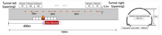
Figure 1.
Longitudinal view of the model tunnel geometry and an example fire scenario used in the CFD simulations. The tunnel is 1500 m long with a midspan height of 7.5 m, and sensors are mounted 7 m above the roadway surface at 20 m intervals, yielding a total of 75 measurement points along the tunnel axis. The illustrated case corresponds to a fire source located 400 m downstream from the left tunnel portal.

Table 1.
Fire case scenarios with combinations of heat release rates and growth rates.
2.3. Dataset Construction and Preprocessing
We construct our dataset from three-dimensional CFD simulations of fire spread in a tunnel environment. In total, we simulate 108 distinct fire scenarios, each running for . During each simulation, physical quantities are recorded at intervals, resulting in a discrete-time sequence of states for every scenario. At each time step, we collect two types of data: (i) point-wise measurements from a set of sparse sensors, and (ii) full-field distributions over the 3D tunnel domain.
The sensor system consists of fixed measurement locations distributed along the tunnel. At every time step t, each sensor records three physical quantities: temperature, soot concentration, and CO concentration. In parallel, the CFD solver outputs the full three-dimensional fields of the same quantities (temperature, soot, and CO) over the entire tunnel interior. These full-field distributions are used as supervision signals for learning, while the sparse sensor readings serve as model inputs.
The objective of this study is to learn a model that reconstructs and forecasts the global fire state in the tunnel from sparse, time-resolved sensor data. Given a past time window of length t seconds, the model is trained to predict the tunnel-wide fire state at a future time offset seconds. For each training sample, we construct an input tensor
where each row corresponds to one time step in the context window and each column corresponds to a sensor. (When multiple physical variables are used jointly, the feature dimension is extended accordingly, but we denote the core structure as for clarity).
Although the CFD simulations are fully three dimensional, in this work we employ a two-dimensional representation of the target field for both computational efficiency and interpretability in safety-related analysis. Specifically, at the target time , the 3D fields of temperature, soot, and CO are projected onto two physically meaningful cross-sections of the tunnel:
- Vertical mid-plane (longitudinal section): a vertical plane passing through the center of the tunnel, capturing the longitudinal evolution of the fire and smoke along the tunnel axis.
- Horizontal breathing plane: a horizontal plane at the height of the human breathing zone (e.g., approximately above the floor), capturing the conditions that are directly relevant to human exposure.
To make the system deployable on low-cost GPUs and suitable for real-time inference, we deliberately reduce the spatial resolution of these 2D target fields during preprocessing. Each projected field is resampled and downsampled to a fixed grid of resolution , where the first dimension corresponds to the vertical (or cross-sectional) direction and the second dimension follows the tunnel axis (see Figure 2). The model decoder is designedto emit predictions at exactly this reduced resolution, so all label tensors are stored as
In our experiments, we treat the vertical mid-plane and the horizontal breathing plane as two alternative label configurations and train the model on one configuration at a time.
Under this formulation, the learning problem can be written as approximating the mapping
which takes t seconds of historical measurements from 75 sensors and predicts the two-dimensional tunnel fire distribution seconds into the future, either on the vertical mid-plane or on the horizontal breathing plane, for C physical variables (e.g., temperature, soot, and CO). This setup explicitly couples sparse sensor data with reduced, yet safety-critical, projections of the 3D CFD fields and provides a structured benchmark for data-driven fire spread prediction in tunnel environments.
2.4. Proposed 2D ST-FAM
In this study, we introduce 2D ST-FAM (SpatioTemporal Fire spread forecasting AI Model), a data-driven model that predicts the tunnel-wide two-dimensional field distribution from sparse sensor measurements (see Figure 3). The model takes as input a sequence of sensor readings over a past time window of length t seconds and predicts the full 2D field at a future target time . Architecturally, 2D ST-FAM follows an encoder–bottleneck–decoder design composed of a Long Short-Term Memory (LSTM [22]) encoder, a fully connected bottleneck block, and a spatial decoder. The LSTM encoder ingests the time-resolved sparse sensor data and captures the underlying temporal dependencies of the fire dynamics in a latent feature representation. This encoded representation is then transformed by the bottleneck block into a compact latent vector that is well suited for spatial reconstruction. Finally, the decoder maps this latent vector to the full tunnel cross-sectional field on the grid, generating the predicted each scalar field (temperature, soot, CO) distributions at the future time offset . The detailed layer-wise architecture of 2D ST-FAM is provided in Appendix B.

Figure 2.
Vertical center plane (longitudinal section) and horizontal breathing plane (1.8 m above the walkway bottom) extracted from the 3D CFD simulation. The center plane shows an example temperature contour and the breathing plane shows an example CO contour, both resampled and downsampled to a resolution of and used as 2D target fields for model training.


Figure 3.
Architecture of the proposed 2D ST-FAM. A sequence of sparse measurements from 75 sensors over a past time window of length t is encoded by stacked LSTM layers and a fully connected bottleneck. The decoder, composed of transposed convolution and convolution blocks, upsamples the latent representation to a 2D field and produces the prediction of the fire-spread state seconds ahead on the chosen tunnel cross-section.

A previous study [16] considered a significantly smaller tunnel configuration: a 160 m long tunnel instrumented with 32 sensors placed at 5 m intervals along the longitudinal axis. The forecasting model employed a relatively compact architecture with two stacked LSTM layers, followed by two fully connected layers, and a transposed-convolutional (TConv [23]) decoder comprising six TConv layers and a final convolutional layer to reconstruct the fire spread fields. This configuration was sufficient to capture the fire dynamics over the smaller domain and sparser spatial extent. Compared to previous work, the present tunnel setting poses a substantially larger spatial domain and a denser sensor configuration. Directly reusing the earlier model architecture in this enlarged setting led to poor convergence and inadequate reconstruction quality, indicating that the original capacity and representation pathway were no longer sufficient. In 2D ST-FAM, we therefore (i) roughly double the number of sensors used as input, (ii) increase the dimensionality of the LSTM hidden state relative to the earlier model to enhance temporal modeling capacity, and (iii) introduce a dedicated fully connected bottleneck block between the recurrent encoder and the spatial decoder. The enlarged LSTM hidden state and the bottleneck block were tuned empirically to strike a balance between expressiveness and stability during training.
The fully connected bottleneck plays a central role in scaling to larger spatial domains. It aggregates the temporally encoded sensor features into a structured latent vector whose size is carefully matched to the spatial decoder’s input shape. This design allows the decoder to exploit the sensor information and expanded receptive field without incurring prohibitive memory or compute costs. By appropriately controlling the dimensionality of this bottleneck, we are able to train 2D ST-FAM to convergence on low-cost GPUs and to maintain real-time inference throughput, while still accurately capturing fire, soot, and CO spread over the enlarged tunnel cross-section.
2.4.1. LSTM-Based Temporal Encoder
The temporal encoder operates on the sequence of sparse measurements collected from the sensors. For each training sample, the input is represented as
where denotes the sensor readings at time step within the past time window of length t seconds. This sequence is fed into the LSTM layers, which are designed to model temporal dependencies in sequential data through gated recurrence. Formally, at each time step , the LSTM updates its hidden state and cell state based on the current input and the previous states . Through this recurrent update, the LSTM-based encoder integrates information across the entire input window and captures the underlying, non-linear temporal evolution of the fire dynamics as observed by the sparse sensors. We use the final hidden state (or its projection in the case of stacked layers) as a compact temporal embedding, which summarizes the history of sensor measurements and serves as the input to the subsequent dense bottleneck layer.
2.4.2. Fully Connected Bottleneck Block
The fully connected bottleneck block bridges the LSTM-based temporal encoder and the spatial decoder. It receives the final hidden state from the temporal encoder and transforms it into a low-resolution spatial feature map that can be processed by the decoder. Concretely, the bottleneck block consists of four fully connected layers with nonlinear activations. The first layer maps the encoded temporal feature to an intermediate representation of dimension S, where is the number of sensors. This step can be interpreted as re-expressing the temporal information in a sensor-aligned feature space, in which the contribution of each sensor to the global fire dynamics is reweighted and combined. The subsequent three layers progressively increase the feature dimension and project the representation to a target size of . The final output of the bottleneck block is then reshaped into a tensor
which serves as the input to the spatial decoder. From a functional point of view, the bottleneck block acts as a nonlinear mapping that converts the one-dimensional temporal embedding into a compact spatio-temporal latent field. It retains the essential information about the global fire-spread state (e.g., overall fire intensity and the coarse location of the fire front along the tunnel), while constraining the representation to a limited spatial resolution. This information bottleneck regularizes the model, reducing the risk of overfitting to the high-dimensional CFD outputs and providing a structured latent representation that can be efficiently upsampled by the decoder to the full field.
2.4.3. Transposed Convolutional Decoder
The transposed convolutional decoder takes the bottleneck tensor as input and reconstructs the full tunnel cross-sectional field on the grid. The decoder is implemented as a sequence of six transposed convolutional (TConv) layers followed by a final convolutional (Conv) layer. Each TConv layer performs a learned upsampling step, progressively increasing the spatial resolution of the feature maps from the low-resolution latent field to the target resolution, while the intermediate nonlinearities enable the model to capture complex spatial patterns.
After the six TConv layers have expanded the spatial dimensions to match the grid, the final Conv layer acts as a projection head that maps the decoder features to C output channels, corresponding to the predicted each scalar (temperature, soot, CO) field on the chosen tunnel cross-section. In this way, the decoder propagates the global information encoded in the bottleneck representation across the entire spatial domain, while still recovering fine-scale spatial structures that are critical for assessing the fire-spread state seconds ahead.
2.5. Training Details
2.5.1. Data Splits and Sample Construction
For each of the 108 CFD simulation scenarios, we construct supervised training samples by sliding a temporal window of length t over the sensor sequences with a stride of s seconds. For each window, we pair the past sensor measurements with the corresponding 2D target field at the future time , as described in Section 2.2. The resulting dataset is partitioned into training, validation, and test sets on a scenario basis, ensuring that no scenario appears in more than one split. We adopt an 8:1:1 split ratio over the 108 scenarios, resulting in scenarios for training, for validation, and for testing. This setup evaluates the ability of the model to generalize to unseen fire scenarios rather than to previously seen time segments of the same scenario. In all experiments, we set the input window length to and the prediction horizon to , with a stride of between consecutive samples.
2.5.2. Loss Function and Optimization
We train 2D ST-FAM in a supervised fashion by minimizing the discrepancy between the predicted and ground-truth fields. In this work, we focus on single-channel prediction: for each physical quantity (temperature, soot, or CO), we train a separate instance of 2D ST-FAM using only the corresponding field as the target. Accordingly, the loss function is defined as the mean squared error (MSE) over all spatial locations,
where and denote the spatial dimensions of the 2D field. For completeness, we also report results with a combined loss that includes a structural similarity (SSIM) term to emphasize the structural fidelity of the predicted single-channel fields.
The model parameters are optimized using the Adam optimizer with an initial learning rate of and default momentum parameters . We use a mini-batch size of and train the model for up to epochs.
2.5.3. Learning Schedule and Regularization
To stabilize training and avoid overfitting, we employ early stopping based on the validation loss with a patience of epochs. Although the maximum number of training epochs is set to 500, training typically terminates much earlier; in our experiments, early stopping halted training after 114 epochs.
We use an exponential learning rate scheduler (ExponentialLR) on top of the Adam optimizer, with a decay factor of applied at every epoch to the initial learning rate . Weight decay is handled via the regularization term implemented in the Adam optimizer with its default coefficient. Unless otherwise noted, dropout is not used in the LSTM or dense layers, as we did not observe consistent benefits in our experiments.
2.5.4. Implementation Details
All models are implemented in PyTorch v2.7.1 and trained on a workstation equipped with two NVIDIA RTX 3090 GPUs and 64 GB of RAM. All experiments reported in this paper are conducted on a single GPU using single-precision floating point (FP32) arithmetic for both training and inference. During training, the input sensor sequences and target fields are linearly scaled to the range using min–max normalization, where the minimum and maximum values are computed from the training set only; the same scaling parameters are then applied to the validation and test sets.
2.6. Evaluation Metrics
To quantitatively assess the performance of 2D ST-FAM, we compare the predicted fields with the CFD-based ground-truth fields Y obtained from the simulations. During training, the model parameters are optimized using a pixel-wise mean squared error (MSE) loss. For evaluation and model comparison, however, we primarily report the structural similarity index (SSIM), which is designed to reflect perceptual and structural differences between two images rather than purely point-wise errors. Unless otherwise stated, all metrics are computed per sample over the full spatial domain and then averaged over all samples in the test set, separately for each physical quantity (temperature, soot, or CO).
Structural Similarity Metric
While pixel-wise errors such as MSE capture the average magnitude of point-wise discrepancies, they do not directly reflect the structural quality of the predicted fields. In the context of tunnel fire safety, the spatial patterns and extent of high-temperature or high-concentration regions are often more critical than purely local differences. To evaluate the preservation of such spatial structures, we therefore rely primarily on the structural similarity index (SSIM) between the predicted and ground-truth fields.
For a given sample and a given 2D field, SSIM is defined as
where and are the mean intensities of the ground-truth and predicted fields, and are their variances, and is the covariance between them. The constants and are small positive values that stabilize the division. In this formulation, SSIM jointly compares luminance (mean intensity), contrast (variance), and structural similarity (normalized correlation) between Y and , thereby providing a perceptually motivated assessment of image quality. We report the average SSIM over all test samples, separately for each physical quantity, and use it as the primary metric to compare different models and configurations.
3. Results
3.1. Overall Prediction Performance
We evaluate 2D ST-FAM on three physical quantities—temperature, soot, and CO—and on two different cross-sectional configurations: (i) the vertical center plane along the tunnel axis (center plane, longitudinal section), and (ii) the horizontal breathing plane at human breathing height (breathing plane, horizontal section). For each configuration and physical quantity, we compute the structural similarity index (SSIM) between the predicted 2D field and the CFD-based ground-truth field Y over the full prediction period of . SSIM values are first computed at each time step and then averaged over all time steps and test scenarios. This quantitative analysis is used to answer RQ1–RQ3 by assessing overall reconstruction fidelity, cross-plane consistency, and performance differences across physical quantities.
Table 2 summarizes the resulting average SSIM scores for each physical quantity, aggregated over both cross-sectional planes. Overall, 2D ST-FAM achieves an SSIM of for temperature, for CO, and for soot, indicating consistently high structural agreement with the CFD reference fields. Previous image quality studies have reported that SSIM values on the order of and above typically correspond to images that are perceptually indistinguishable or very difficult to dichotomize for human observers, i.e., visually lossless reconstructions. (Several works in image quality assessment and medical imaging report that combinations of high PSNR (e.g., >40 dB) and SSIM ≳ 0.98 correspond to perceptually indistinguishable image pairs.) In this context, the CO field with an SSIM of lies in the visually near-lossless regime, while the temperature and soot fields also exhibit very high similarity, with only minor but perceptible differences remaining in the most challenging regions. Taken together, these values support H1: the model reproduces the dominant structure of the future tunnel field from sparse sensor histories.
Table 2.
SSIM for each data type on the center and breathing planes.
The plane-specific results further clarify the behavior of the model. For temperature, the center-plane SSIM is and the breathing-plane SSIM is , indicating similarly strong performance on both target sections. For CO, the model reaches on the center plane and on the breathing plane, again showing stable reconstruction quality across views. Soot is the most challenging quantity, with SSIM values of on the center plane and on the breathing plane, but even here the model preserves the main plume structure. These comparisons support H2 by showing that the forecasting framework remains effective on both planes, and they support H3 by showing that soot prediction is consistently less accurate than temperature and CO prediction under the same experimental conditions.
3.2. Qualitative Comparison on Center and Breathing Planes
To complement the SSIM-based quantitative evaluation, we provide qualitative visualizations comparing the predicted fields with the CFD ground-truth fields on both the center plane and the breathing plane. Figure 4 show representative snapshots at , , and for each physical quantity. For each timestamp and quantity, the CFD field and the corresponding 2D ST-FAM prediction are displayed side by side, using the same colormap and dynamic range to enable a direct visual comparison.
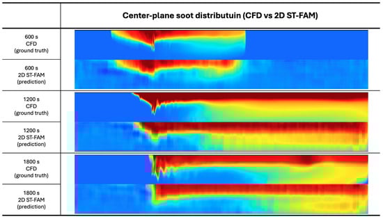
Figure 4.
Qualitative comparison between CFD ground truth and 2D ST-FAM predictions on the vertical center plane for temperature, soot, and CO at , , and . For each quantity and time instant, the CFD field (left) and the predicted field (right) are shown with the same colormap and value range.
On the vertical center plane, the predicted temperature fields closely match the extent and shape of the high-temperature regions along the tunnel, and the CO and soot predictions accurately track the growth and downstream transport of the smoke and gas plumes. On the horizontal breathing plane, the model successfully reproduces the lateral spread and intensity distribution within the human breathing zone, which is critical for safety assessment. Across all three time instants (600, 1200, and ), the predicted fields exhibit very similar large-scale structures and gradients to the CFD fields, with discrepancies mainly confined to fine-scale details near steep fronts or highly localized concentrations. These qualitative observations are consistent with the high SSIM scores reported in Table 2 and support the conclusion that 2D ST-FAM can reliably reconstruct the tunnel-wide fire state on both cross-sectional planes over the entire evolution. They also sharpen the quantitative interpretation: the model is strongest at recovering global plume extent, downstream transport, and broad concentration gradients, whereas local peak structure remains more challenging in the sharper soot fields.
4. Discussion
In this work, we proposed 2D ST-FAM, a data-driven model for forecasting the tunnel-wide fire state from sparse sensor measurements. Over the entire prediction horizon of , 2D ST-FAM achieves average SSIM values of for temperature, for CO, and for soot, indicating that the model is able to reconstruct the global field structure with high fidelity. The model performs consistently well on both the vertical center plane and the horizontal breathing plane, suggesting that the learned mapping from sparse sensor histories to 2D fields generalizes across physically distinct cross-sections that are relevant for structural integrity (center plane) and human safety (breathing plane).
These findings answer the research questions posed in Section 2. First, RQ1 is answered positively within the scope of the simulated dataset: sparse sensor histories contain enough information for the model to reconstruct future tunnel-wide temperature, soot, and CO fields with high structural fidelity. Second, RQ2 is also answered positively, because the model remains effective on both the center plane and the breathing plane. Third, RQ3 is answered by the observed performance ranking, with soot consistently harder to predict than temperature and CO.
The performance gap between temperature/CO and soot is physically plausible and highlights an important limitation of the current architecture. Temperature and CO fields in the considered scenarios exhibit relatively smooth spatial patterns that are dominated by diffusion and large-scale advection, which are well captured by the LSTM encoder and convolutional decoder. In contrast, soot concentration forms sharp, filamentary plumes that are strongly influenced by turbulent mixing and small-scale flow structures. These fine-scale, highly nonlinear dynamics are harder to infer from sparse measurements and are more sensitive to small errors in the latent representation, which is reflected in the lower SSIM scores for soot, particularly on the center plane. Nevertheless, the soot SSIM remains in a regime that preserves the main plume extent and transport direction, which is often the primary concern for tunnel smoke management.
A key practical advantage of 2D ST-FAM is its computational efficiency and flexibility in inference resolution. Once trained, the model can generate tunnel-wide 2D fields in a single forward pass, with a computational cost that is orders of magnitude lower than running a full CFD simulation. In our setup, a single 1800 s tunnel fire scenario requires more than six hours of wall-clock time for the CFD solver to complete, highlighting the substantial gain in efficiency provided by the proposed surrogate. Moreover, the decoder architecture allows the output resolution to be adjusted, enabling deployments on lower-specification GPUs while still covering longer tunnel sections than those typically feasible with traditional surrogate models. In operational settings where real-time or near-real-time assessments of the fire state are required, the proposed approach can therefore serve as a fast surrogate to CFD, providing spatially resolved temperature, soot, and CO fields from live sensor data and supporting ventilation control or evacuation decision-making.
At the same time, the present evidence should be interpreted with appropriate boundaries. The evaluation is based on CFD-generated scenarios rather than field measurements from operating tunnels, and the reported performance does not by itself establish robustness to tunnel geometries, ventilation patterns, or fire conditions outside the simulated range. Similarly, because this study does not compare multiple model families under a unified benchmark, the results support the effectiveness of 2D ST-FAM on the present dataset but do not by themselves justify broader superiority claims beyond that scope.
Future work will focus on improving the representation of particle-laden flows such as soot. This may include enriching the model with multi-scale or attention-based components, incorporating additional physical constraints (e.g., mass conservation or plume transport priors), or designing loss functions that explicitly emphasize sharp fronts and localized high-concentration regions. Beyond 2D cross-sections, an important next step is to extend the framework to three-dimensional forecasting of the fire state in full building or tunnel geometries, enabling the prediction of inter-floor or inter-compartment spread. Such 3D extensions, combined with more diverse CFD datasets and varying tunnel and building configurations, would further enhance the robustness and applicability of data-driven fire-spread forecasting models in real-world safety-critical environments.
5. Conclusions
In this work, we presented 2D ST-FAM, a data-driven model for forecasting the fire state in road tunnels from sparse sensor measurements. Building on a CFD dataset of 108 tunnel fire scenarios with a temporal resolution of over , we formulated a supervised learning framework in which the model receives a past window of sensor histories and predicts the future tunnel field on physically meaningful 2D cross-sections (the vertical center plane and the horizontal breathing plane). 2D ST-FAM follows an encoder–bottleneck–decoder design: an LSTM-based temporal encoder aggregates the histories from 75 sensors, a fully connected bottleneck block maps the temporal embedding to a compact spatio-temporal latent representation, and a transposed convolutional decoder reconstructs a field on the chosen cross-section. Across all test scenarios and the full horizon, the model attains average SSIM scores of for temperature, for CO, and for soot, indicating a high level of structural agreement with the CFD-based reference fields. These results are consistent on both the center and breathing planes, suggesting that the learned mapping from sparse sensor histories to spatially resolved fields generalizes across cross-sections that are critical for both structural assessment and human safety. Although soot remains more challenging due to its filamentary, turbulence-driven plume structure, 2D ST-FAM still preserves the main extent and downstream transport of the soot plume, which are key quantities for practical smoke management in tunnels.
A further advantage of 2D ST-FAM lies in its computational efficiency and flexible inference resolution. Once trained, the model produces tunnel-wide 2D fields in a single forward pass, at a computational cost several orders of magnitude lower than that of a full CFD simulation, enabling real-time or near-real-time deployment in the simulated setting considered here. The decoder design allows the output resolution to be adapted to the available hardware budget, making it possible to cover long tunnel sections even on comparatively modest GPUs and to use 2D ST-FAM as a surrogate model that can be coupled with live sensor streams to support ventilation control and evacuation decision-making. Future work will focus on improving the representation of particle-laden flows such as soot, for example through multi-scale architectures, attention mechanisms, or physics-informed loss terms that better capture fine-scale turbulent structures. Extending the framework from 2D cross-sections to full 3D geometries, and training on more diverse CFD datasets and infrastructure configurations, will be important steps towards robust, data-driven fire-spread forecasting systems that can be applied in real-world safety-critical environments.
Author Contributions
Conceptualization, J.O. and K.L.; methodology, J.O. and K.L.; software, J.O. and Y.K.; validation, J.O. and Y.K.; formal analysis, S.C. and Y.K.; Investigation, D.L., T.K. and J.K.; resources, K.L.; Data curation, Y.K., S.C. and S.H.; writing—original draft preparation, S.C. and Y.K.; writing—review and editing, Y.K.; visualization, Y.K.; supervision, K.L.; project administration, K.L.; funding acquisition, K.L. All authors have read and agreed to the published version of the manuscript.
Funding
This work was supported by the Korea Agency for Infrastructure Technology Advancement (KAIA) grant funded by the Ministry of Land, Infrastructure and Transport (Grant No. RS-2023-00238018).
Data Availability Statement
The raw data supporting the conclusions of this article will be made available by the authors on request.
Conflicts of Interest
Authors Yoonseok Kim, Stephen Cha, Jaehwan Oh and Kyohyuk Lee were employed by the company Kaier Corporation. Author Seokwoo Hong was employed by the company FNS English, Inc. The remaining authors declare that the research was conducted in the absence of any commercial or financial relationships that could be construed as a potential conflict of interest.
Abbreviations
The following abbreviations are used in this manuscript:
| 2D ST-FAM | Two-Dimensional SpatioTemporal Fire Spread Forecasting AI Model |
| CFD | Computational Fluid Dynamics |
| LSTM | Long Short-Term Memory |
| SSIM | Structural Similarity Index |
| MSE | Mean Squared Error |
| CO | Carbon Monoxide |
| GPU | Graphics Processing Unit |
| CFD-GT | CFD Ground Truth |
Appendix A
This appendix presents additional qualitative results of the proposed 2D ST-FAM model for the same tunnel fire scenario as in Figure 4. For this scenario, we visualize the predicted temperature, soot, and CO concentration fields on both the vertical center plane and the horizontal breathing plane, and compare them against the corresponding CFD reference fields.
Figure A1 and Figure A2 show the evolution of the predicted fields on the vertical center plane for temperature, soot, and CO, respectively. Each figure includes multiple time snapshots at increasing time offsets , illustrating the ability of 2D ST-FAM to track the longitudinal progression of the fire front, hot gas layer, and toxic gas plume along the tunnel axis. The predicted patterns closely follow the CFD reference in terms of both spatial extent and intensity, with only minor local deviations near sharp gradients.
Figure A3 and Figure A5 display the corresponding predictions on the horizontal breathing plane. These visualizations highlight the conditions most relevant to human exposure, such as walkable temperature ranges and regions of elevated CO concentration in the vicinity of evacuation paths. The breathing-plane results further confirm that the model can reproduce the complex spatio-temporal structure of the CFD fields at the reduced resolution of , while remaining suitable for real-time inference on low-cost GPUs. Overall, the qualitative agreement between the predicted and reference fields across temperature, soot, and CO indicates that 2D ST-FAM captures the key dynamics required for evacuation-oriented fire spread forecasting in tunnel environments.

Figure A1.
Predicted and reference temperature fields on the vertical center plane for the same tunnel fire scenario as in Figure 4. Multiple time snapshots at increasing are shown, illustrating the longitudinal progression of the hot gas layer along the tunnel axis.
Figure A1.
Predicted and reference temperature fields on the vertical center plane for the same tunnel fire scenario as in Figure 4. Multiple time snapshots at increasing are shown, illustrating the longitudinal progression of the hot gas layer along the tunnel axis.


Figure A2.
Predicted and reference CO concentration fields on the vertical center plane for the Figure 4 scenario. The plume of toxic gas is accurately captured in both its downstream spread and vertical stratification.
Figure A2.
Predicted and reference CO concentration fields on the vertical center plane for the Figure 4 scenario. The plume of toxic gas is accurately captured in both its downstream spread and vertical stratification.


Figure A3.
Predicted and reference temperature and soot concentration fields on the horizontal breathing plane (1.8 m above the walkway bottom) for the Figure 4 scenario. These visualizations highlight the evolution of walkable temperature regions and smoke-affected zones along potential evacuation paths.


Figure A4.
Predicted and reference CO concentration fields on the horizontal breathing plane for the Figure 4 scenario. High-CO regions are clearly delineated, demonstrating the model’s ability to reproduce toxic gas exposure patterns at the breathing level.
Figure A4.
Predicted and reference CO concentration fields on the horizontal breathing plane for the Figure 4 scenario. High-CO regions are clearly delineated, demonstrating the model’s ability to reproduce toxic gas exposure patterns at the breathing level.


Figure A5.
Predicted and reference soot concentration fields on the horizontal breathing plane for the Figure 4 scenario. Soot regions are clearly delineated, demonstrating the model’s ability to reproduce toxic gas exposure patterns at the breathing level.
Figure A5.
Predicted and reference soot concentration fields on the horizontal breathing plane for the Figure 4 scenario. Soot regions are clearly delineated, demonstrating the model’s ability to reproduce toxic gas exposure patterns at the breathing level.

Appendix B
This appendix summarizes the detailed layer-wise architecture of the proposed 2D ST-FAM model. Table A1, Table A2 and Table A3 list the configurations of the LSTM encoder, the fully connected bottleneck block, and the spatial decoder used in all experiments.
Table A1.
Layer-wise configuration of the LSTM encoder in 2D ST-FAM.
Table A1.
Layer-wise configuration of the LSTM encoder in 2D ST-FAM.
| Layer | Description | Input Shape | Output Shape | Dropout |
|---|---|---|---|---|
| 1 | LSTM 1 | |||
| 2 | LSTM 2 | 0 | ||
| 3 | Temporal aggregation (last hidden state) | 0 |
Table A2.
Configuration of the fully connected bottleneck block.
Table A2.
Configuration of the fully connected bottleneck block.
| Layer | Description | Input Dim. | Output Dim. |
|---|---|---|---|
| 1 | Fully connected + nonlinearity | 30 | 75 |
| 2 | Fully connected + nonlinearity | 75 | 156 |
| 3 | Fully connected + nonlinearity | 156 | 312 |
| 4 | Fully connected + nonlinearity | 312 | 552 |
Table A3.
Layer-wise configuration of the spatial decoder in 2D ST-FAM.
Table A3.
Layer-wise configuration of the spatial decoder in 2D ST-FAM.
| Block | Layer Type | Kernel/Stride | Input Shape | Output Shape |
|---|---|---|---|---|
| 1 | FC reshape to feature map | – | 552 | |
| 2 | TConv block 1 | |||
| 3 | TConv block 2 | |||
| 4 | TConv block 3 | |||
| 5 | TConv block 4 | |||
| 6 | TConv block 5 | |||
| 7 | TConv block 6 | |||
| 8 | Final Conv |
References
- Doerr, S.H.; Santín, C. Global trends in wildfire and its impacts: Perceptions versus realities in a changing world. Philos. Trans. R. Soc. B Biol. Sci. 2016, 371, 20150345. [Google Scholar] [CrossRef] [PubMed]
- Jones, M.W.; Abatzoglou, J.T.; Veraverbeke, S.; Andela, N.; Lasslop, G.; Forkel, M.; Smith, A.J.P.; Burton, C.; Betts, R.A.; van der Werf, G.R.; et al. Global and regional trends and drivers of fire under climate change. Rev. Geophys. 2022, 60, e2020RG000726. [Google Scholar] [CrossRef]
- Kelley, D.I.; Burton, C.; Di Giuseppe, F.; Jones, M.W.; Barbosa, M.L.; Brambleby, E.; McNorton, J.R.; Liu, Z.; Bradley, A.S.I.; Blackford, K.; et al. State of Wildfires 2024–2025. Earth Syst. Sci. Data 2025, 17, 5377–5488. [Google Scholar] [CrossRef]
- Knorr, W.; Kaminski, T.; Arneth, A.; Weber, U. Impact of human population density on fire frequency at the global scale. Biogeosciences 2014, 11, 1085–1102. [Google Scholar] [CrossRef]
- Xu, H.; Zlatanova, S.; Liang, R.; Canbulat, I. Generative AI as a Pillar for Predicting 2D and 3D Wildfire Spread: Beyond Physics-Based Models and Traditional Deep Learning. Fire 2025, 8, 293. [Google Scholar] [CrossRef]
- Chen, J.; Long, Z.; Wang, L.; Xu, B.; Bai, Q.; Zhang, Y.; Liu, C.; Zhong, M. Fire evacuation strategy analysis in long metro tunnels. Saf. Sci. 2022, 147, 105603. [Google Scholar] [CrossRef]
- Wang, Z.; Mao, Z.; Li, Y.; Yu, L.; Zou, L. VR-based fire evacuation in underground rail station considering staff’s behaviors: Model, system development and experiment. Virtual Real. 2023, 27, 1145–1155. [Google Scholar] [CrossRef]
- Sun, J.; Lu, Z.; Zhou, D. Optimization analysis of evacuation facility parameters in interval tunnels under subway train fire accidents. Physica A 2024, 651, 130020. [Google Scholar] [CrossRef]
- Zhang, N.; Liang, Y.; Zhou, C.; Niu, M.; Wan, F. Study on fire smoke distribution and safety evacuation of subway station based on BIM. Appl. Sci. 2022, 12, 12808. [Google Scholar] [CrossRef]
- Chow, W.K.; Lam, K.C.; Fong, N.K.; Li, S.S.; Gao, Y. Numerical simulations for a typical train fire in China. Model. Simul. Eng. 2011, 2011, 369470. [Google Scholar] [CrossRef]
- Bi, H.; Zhou, Y.; Wang, H.; Gou, Q.; Liu, X. Characteristics of fire in high-speed train carriages. J. Fire Sci. 2020, 38, 75–95. [Google Scholar] [CrossRef]
- Du, H.; Tang, Z.; Meng, S.; Zhou, D. Tunnel shaft impact on smoke transport in fire-induced high-speed train stopping. Phys. Fluids 2025, 37, 025144. [Google Scholar] [CrossRef]
- Lattimer, B.Y.; Hodges, J.L.; Lattimer, A.M. Using machine learning in physics-based simulation of fire. Fire Saf. J. 2020, 114, 102991. [Google Scholar] [CrossRef]
- Zeng, Y.; Zhang, X.; Su, L.C.; Wu, X.; Xinyan, H. Artificial intelligence tool for fire safety design (IFETool): Demonstration in large open spaces. Case Stud. Therm. Eng. 2022, 40, 102483. [Google Scholar] [CrossRef]
- Zhang, X.; Wu, X.; Park, Y.; Zhang, T.; Huang, X.; Xiao, F.; Usmani, A. Perspectives of big experimental database and artificial intelligence in tunnel fire research. Tunn. Undergr. Space Technol. 2021, 108, 103691. [Google Scholar] [CrossRef]
- Wu, X.; Zhang, X.; Huang, X.; Xiao, F.; Usmani, A. A real-time forecast of tunnel fire based on numerical database and artificial intelligence. Build. Simul. 2022, 15, 511–524. [Google Scholar] [CrossRef]
- Zhang, L.; Mo, L.; Fan, C.; Zhou, H.; Zhao, Y. Data-driven prediction methods for real-time indoor fire scenario inferences. Fire 2023, 6, 401. [Google Scholar] [CrossRef]
- Zeng, Y.; Zheng, Z.; Zhang, T.; Huang, X.; Lu, X. AI-powered fire engineering design and smoke flow analysis for complex-shaped buildings. J. Comput. Des. Eng. 2024, 11, 359–373. [Google Scholar] [CrossRef]
- Lee, K.-Y.; Kim, J.-S.; Jeong, J.-M. Fire spreading prediction based on spatio-temporal neural network model. J. IKEEE 2025, 29, 101–107. [Google Scholar]
- Brunton, S.L.; Proctor, J.L.; Kutz, J.N. Discovering governing equations from data by sparse identification of nonlinear dynamical systems. Proc. Natl. Acad. Sci. USA 2016, 113, 3932–3937. [Google Scholar] [CrossRef]
- Yermakov, A.; Zoro, D.; Gao, M.L.; Kutz, J.N. T-SHRED: Symbolic Regression for Regularization and Model Discovery with Transformer Shallow Recurrent Decoders. arXiv 2025, arXiv:2506.15881. [Google Scholar] [CrossRef]
- Hochreiter, S.; Schmidhuber, J. Long Short-Term Memory. Neural Comput. 1997, 9, 1735–1780. [Google Scholar] [CrossRef]
- Long, J.; Shelhamer, E.; Darrell, T. Fully Convolutional Networks for Semantic Segmentation. In Proceedings of the 2015 IEEE Conference on Computer Vision and Pattern Recognition (CVPR), Boston, MA, USA, 7–12 June 2015; pp. 3431–3440. [Google Scholar]


Disclaimer/Publisher’s Note: The statements, opinions and data contained in all publications are solely those of the individual author(s) and contributor(s) and not of MDPI and/or the editor(s). MDPI and/or the editor(s) disclaim responsibility for any injury to people or property resulting from any ideas, methods, instructions or products referred to in the content. |
© 2026 by the authors. Licensee MDPI, Basel, Switzerland. This article is an open access article distributed under the terms and conditions of the Creative Commons Attribution (CC BY) license.