Article

A Joint Transformer–XGBoost Model for Satellite Fire Detection in Yunnan

1
Electric Power Research Institute, Yunnan Power Grid Co., Ltd., China Southern Power Grid, Kunming 650220, China
2
Department of Mechanical Engineering, Baoding Campus, North China Electric Power University, Baoding 071003, China
3
School of Energy Power and Mechanical Engineering, Beijing Campus, North China Electric Power University, Beijing 102206, China
*
Author to whom correspondence should be addressed.
Fire 2025, 8(10), 376; https://doi.org/10.3390/fire8100376
Submission received: 28 August 2025 / Revised: 18 September 2025 / Accepted: 22 September 2025 / Published: 23 September 2025

Abstract

Wildfires pose a regularly increasing threat to ecosystems and critical infrastructure. The severity of this threat is steadily increasing. The growing threat necessitates the development of technologies for rapid and accurate early detection. However, the prevailing fire point detection algorithms, including several deep learning models, are generally constrained by the inherent hard threshold limitations in their decision-making logic. As a result, these methods lack adaptability and robustness in complex and dynamic real-world scenarios. To address this challenge, the present paper proposes an innovative two-stage, semi-supervised anomaly detection framework. The framework initially employs a Transformer-based autoencoder, which serves to transform raw fire-free time-series data derived from satellite imagery into a multidimensional deep anomaly feature vector. Self-supervised learning achieves this transformation by incorporating both reconstruction error and latent space distance. In the subsequent stage, a semi-supervised XGBoost classifier, trained using an iterative pseudo-labeling strategy, learns and constructs an adaptive nonlinear decision boundary in this high-dimensional anomaly feature space to achieve the final fire point judgment. In a thorough validation process involving multiple real-world fire cases in Yunnan Province, China, the framework attained an F1 score of 0.88, signifying a performance enhancement exceeding 30% in comparison to conventional deep learning baseline models that employ fixed thresholds. The experimental results demonstrate that by decoupling feature learning from classification decision-making and introducing an adaptive decision mechanism, this framework provides a more robust and scalable new paradigm for constructing next-generation high-precision, high-efficiency wildfire monitoring and early warning systems.

1. Introduction

In recent years, high-frequency Earth observation satellites (e.g., Himawari, GOES-R, FY-4) have been capable of providing continuous multispectral time-series data with revisit intervals of 5–15 min [1], thereby establishing a novel observational foundation for early fire detection [2]. Nevertheless, the automatic identification of satellite fire points still faces several fundamental challenges: Firstly, the presence of weak fire signals at the pixel scale is often obscured by background noise. To address this challenge, researchers have employed multi-spectral algorithms and spatial context analysis to enhance the fire signature. Secondly, surface heterogeneity and complex land cover types have been shown to increase false alarm rates. This problem has been traditionally addressed by developing region-specific thresholds or applying land-cover masks. These rule-based approaches ultimately encounter difficulties in creating the third, most critical component: long-term, widely applicable decision rules. This limitation severely restricts their ability to generalize across different domains [3].
In order to surmount the constraints imposed by these rule-based methodologies, the integration of deep learning algorithms has precipitated a substantial paradigm shift in the domain of satellite-based fire detection. Early models primarily utilized Convolutional Neural Networks (CNN), with specialized variants such as U-Net and DenseNet proving effective at capturing the spatial features of fire and smoke from satellite imagery. In recent developments, the focus has shifted to temporal dynamics, with the employment of Recurrent Neural Networks (RNN) and Long Short-Term Memory (LSTM) networks to model fire behavior over time using high-frequency data [4]. Recent advancements have given rise to Transformer architectures, which have exhibited superior performance by capturing long-range temporal dependencies in imagery from geostationary satellites.
The efficacy of these deep learning approaches has been demonstrated by their consistent superiority in achieving higher accuracy and lower false alarm rates when compared to traditional threshold-based methods.
Although deep learning-based temporal models (e.g., CNN, GRU, LSTM) can partially extract temporal information [5], most methods still rely on static or manually set decision boundaries, which limits their adaptability and generalisation capabilities.
The objective of this study is to address the aforementioned issues by replacing traditional fixed thresholds with data-driven approaches [6]. The proposed end-to-end framework aims to balance long-term temporal representation capabilities with decision adaptability. The framework is designed to enhance the representation of long-range temporal dependencies and subtle anomaly patterns through attention mechanisms. In addition, it aims to address decision reliability under sparse labeling via structured machine learning and semi-supervised strategies [7,8]. For the purposes of result validation and regional applicability testing, Yunnan Province is employed as the verification case (the research area and data details of which are set out in Section 2).
The primary methods and innovations proposed in this paper include:
Firstly, a Transformer-based autoencoder is employed to learn deep representations rich in long-range correlations from high-frequency satellite time series. Secondly, XGBoost is combined with semi-supervised training to design a classifier with adaptive decision boundaries, enabling robust fire/non-fire classification in structured feature spaces. Finally, an iterative pseudo-labeling strategy is introduced to fully leverage large unlabeled samples [9], mitigating the performance constraints imposed by positive sample scarcity.
Empirical findings in Yunnan demonstrate that the proposed method attains substantial enhancements over several baseline approaches in terms of F1 score (relative gain of approximately 30%), thereby underscoring its efficacy in facilitating early warning systems in complex terrain and diverse vegetation conditions. The integration of attention-driven temporal representations with adaptive, semi-supervised decision mechanisms represents a significant advancement in high-frequency satellite fire hotspot early warning methods, enhancing both generalisation and practical applicability.

2. Study Area and Data

2.1. Study Area

Yunnan Province, located in southwestern China, has been selected as the study area due to its complex topography, high forest cover, and pronounced wet–dry seasonality, which collectively generate some of the country’s highest incidences of wildfire. The dry season, which occurs from November to April, is characterised by a paucity of precipitation and an elevated fire risk. The topography is mountainous, and the land cover is heterogeneous, both of which complicate the behaviour of fires and constrain ground-based suppression efforts. These fires pose a threat not only to the ecosystem but also to the stability of the power grid, particularly in mountainous regions. Wildfires cause significant damage to high-voltage transmission lines through direct combustion, reduction in air insulation, and flashovers caused by smoke particles adhering to insulators, potentially resulting in power outages and cascading failures. Representative fire scenes from the region are displayed in Figure 1.
The combination of these physical and climatic conditions renders Yunnan an optimal natural experimental field for the validation of high-precision, high-frequency fire-point detection algorithms. The present study utilises multi-source data with geostationary satellite imagery Himawari-8/9 as the primary observational input, complemented by multi-source fire-point reference products for model training and validation. A summary of dataset characteristics is provided in Table 1. The combination of frequent satellite revisits, complex terrain, and varied land cover provides a rigorous test bed for evaluating the robustness and generalisability of data-driven detection methods.

2.2. Data Sources

2.2.1. Himawari-8/9

The primary data source for this study is the Advanced Imaging Instrument (AHI) aboard the Japanese Himawari-8/9 geostationary satellites. The AHI has the capacity to observe at a frequency of once every 10 min, thereby providing critical data for capturing the early dynamics of fires. The AHI is equipped with 16 spectral bands that span the visible to thermal infrared range. The thermal infrared bands, which are utilized for fire spot detection, possess a spatial resolution of 2 km. Table 2 lists the technical specifications of the key bands used in this study.

2.2.2. Fire Point Reference Product

To guarantee the validity and reliability of the model, this study established a multi-source fire point labeling system.
The Yunnan Electric Power Research Institute of China Southern Power Grid confirmed the veracity of the fire point records. These records are sourced from the internal records of the Yunnan Electric Power Research Institute of China Southern Power Grid, have undergone a series of verifications, and serve as the benchmark positive samples for model training, ensuring a high degree of relevance to the application scenario.
JAXA WLF L2 Fire Point Product: The Japan Aerospace Exploration Agency (JAXA) has officially released a fire point product. The product is derived from satellite data acquired from the Himawari-8/9 satellite, providing precise information regarding the location of fire points with a temporal resolution of 10 min and a spatial resolution of 2 km. This product serves as a direct comparison reference for evaluating the performance of models [10].
The MODIS 1-km resolution fire point product, also known as MCD14ML, is a key component of the study. This product serves as a long-term benchmark dataset in the field of global fire research. This study uses the product for the cross-comparison and evaluation of algorithm performance [11], selecting fire points with a confidence level greater than 70% from Collection 6 as supplementary labels [12].

3. Fire Point Detection Framework Based on Transformer and XGBoost

3.1. Overall Framework Design

The fire point detection framework proposed in this paper employs a two-stage system for information extraction and refinement. The process commences with feature engineering, wherein raw physical observations (e.g., brightness temperature, reflectance) are transformed into a multidimensional feature time series. This step refines the raw data into high-value features, although the resulting feature space remains complex and highly nonlinear. To address this, the first stage introduces a Transformer-based deep self-encoder. Rather than undertaking a direct classification of data, this stage prioritizes self-supervised learning [13]. This approach utilizes “normal” (non-fire) data to identify intrinsic patterns of surface dynamics [14]. After training, the model functions as a potent feature extractor, converting any given time series into a high-level abstract feature vector [15]. “Anomaly scores” derived from metrics such as “reconstruction error” and “latent space distance” then quantify this vector. This transition marks the shift from physical features to abstract anomaly space, where anomaly signals themselves become new features for analysis.
In this abstract anomaly space, the boundary between fire and non-fire points is theoretically more precise but remains highly complex and nonlinear, exceeding the capability of fixed thresholds. This process culminates in the subsequent stage, where XGBoost, a sophisticated nonlinear classifier, is incorporated. XGBoost autonomously learns a complex decision boundary, accurately identifying fire points in the high-dimensional abstract space. It functions as an “intelligent decision maker,” interpreting the anomaly features generated in the first stage and making the final classification decision.
In summary, each stage of this framework builds on the previous one, creating a logically consistent and complete system, as illustrated in Figure 2.

3.2. Deep Feature Extraction Based on Transformer

3.2.1. Multidimensional Feature Engineering

The primary objective of multidimensional feature engineering is to generate an information-rich input that is sensitive to fire point signals for subsequent Transformer autoencoders. The model is required to acquire an understanding of typical temporal patterns through the analysis of substantial amounts of “normal” data. This process enables the model to identify deviations from these patterns.
The present paper proposes a multidimensional feature set comprising eight physically meaningful features [16,17], which together provide a comprehensive characterization of surface states from multiple dimensions. These dimensions include core thermal anomalies (“heat” signals), surface reflectance changes (“smoke and trace” signals), and mutual verification between these signals (“confirmation” signals). This design guarantees that the input data not only captures direct fire characteristics but also includes corroborating and higher-level logic, thereby enhancing the signal-to-noise ratio.
For each pixel at time t, the following features are computed, resulting in an 8-dimensional feature vector that serves as the time-series input to the Transformer model.
  • A. Thermal anomaly characteristics (“heat” signal)
This set captures direct evidence of a fire in the form of high-intensity thermal radiation from the burning object. This phenomenon serves as the foundation for the process of fire detection, as it facilitates the quantification of thermodynamic anomalies across various dimensions, including the spectral, temporal, and spatial domains.
  • Spectral Differences ( S D );
S D = T 07 T 14
This feature exploits the differential response of the mid-infrared (MIR) band ( T B B 07 , ~3.9 μ m ) and the thermal-infrared (TIR) band ( T B B 07 , ~11.2 μ m ). The MIR band demonstrates a high degree of sensitivity to sub-pixel high-temperature sources, while the TIR band reflects the overall surface temperature with a higher degree of accuracy. In typical atmospheric conditions, the brightness temperatures of ground and clouds are comparable, leading to a stable and low-level spectral difference ( S D ). However, a conflagration results in a marked, nonlinear escalation in the MIR brightness temperature, accompanied by a gradual shift in the TIR band. The observed divergence results in a distinct positive peak in the S D value, thereby serving as a clear anomaly signal.
2.
Robust Temporal Difference ( r T D );
r T D = d d t S a v G o l T B B 07 , t
Normal surface temperature fluctuations, such as diurnal variations, are gradual processes with smooth rates of change. Conversely, fires are sudden events that lead to a significant increase in the MIR brightness temperature over a brief period, resulting in a sharp positive peak in its time derivative. The Savitzky–Golay filter is employed to mitigate sensor noise while preserving the genuine temperature trend, thereby ensuring that the model captures the underlying physical change rather than data artifacts.
3.
Spatial Variance ( S V t );
S V t = T B B 07 , t ( x , y ) ( i , j ) W , ( i , j ) ( x , y ) T B B 07 , t ( i , j ) | W | 1
This feature quantifies the spatial thermal anomaly by calculating the difference between a central pixel’s ( x , y ) MIR brightness temperature ( T B B 07 ) and the mean of its surrounding background pixels within a window W . Crucially, the central pixel itself is excluded from the background mean calculation (hence the | W | 1 denominator). This design prevents the anomaly from being weakened by its own high temperature influencing the background average, thereby ensuring a pristine reference that maximizes the measured deviation and enhances detection sensitivity.
  • B. Reflectance Feature (“Smoke and Traces” Signal)
The fundamental premise underlying this array of features is that fires do not merely generate thermal anomalies; they also profoundly modify the surface’s reflectance characteristics [18]. The capture of reflectance changes induced by post-combustion traces and smoke generated during combustion enables the establishment of an independent evidence chain, thereby significantly enhancing the model’s robustness.
4.
Normalized Difference Fire Index ( N D F I 06 _ 03 );
N D F I 06 _ 03 = R 06 R 03 R 06 + R 03
The underlying physical principle pertains to the observation that fires induce substantial alterations in reflectance within the shortwave infrared (SWIR, ~2.3 μ m ) band and the red light (Red, ~0.64 μ m ) band, exhibiting opposing directions. For the purpose of analyzing vegetation, the reflectance in both the red light and shortwave infrared bands is relatively low and follows predictable seasonal patterns. Consequently, the N D F I value maintains a stable level at a low point. In the aftermath of a conflagration, the ground surface is often charred. On the one hand, elevated temperatures result in desiccation of vegetation and soil, thereby inducing a substantial augmentation in the reflectance of shortwave infrared R 06 , which is highly sensitive to moisture. On the other hand, the substitution of vegetation with black charcoal precipitates a pronounced decline in the reflectance of red light R 03 , which is particularly sensitive to chlorophyll. The substantial opposing change produces a pronounced positive peak in N D F I , indicative of a fundamental shift in the physical characteristics of the surface. This shift is distinctly different from the gradual seasonal variation pattern typically observed.
5.
Smoke Extinction Index ( S E I );
S E I = log mean ( R 03 _ b a c k g r o u n d ) R 03 _ c e n t e r
This index is designed to identify optical anomalies caused by smoke. In optimal conditions, the red-light reflectance R 03 _ c e n t e r of a pixel is closely analogous to its spatial or temporal background mean ( R 03 _ b a c k g r o u n d ) . Consequently, the ratio within the logarithm approaches 1, thereby maintaining the S E I value stable near 0. However, when smoke drifts over the central pixel, aerosol particles scatter and absorb sunlight. This phenomenon obscures the ground surface, leading to a precipitous decline in the measured R 03 _ c e n t e r while the background reflectance remains elevated. The resulting ratio exceeds 1, thereby yielding a substantial positive S E I value.
6.
Shortwave Infrared Anomaly (SWIR Anomaly, S A );
S A = R 06 _ c e n t e r mean ( R 06 _ b a c k g r o u n d )
The structural configuration of this formula mirrors the S V exhibited by the thermal anomaly feature; however, the operational entity pertains to the reflectance within the shortwave infrared R 06 band. The shortwave infrared reflectance of normal ground surfaces is relatively uniform in space, so the difference in reflectance between the central pixel and its neighbors S A is close to zero. The shortwave infrared band 2.3   μ m is capable of reflecting not only ground surface reflectance characteristics but is also highly sensitive to the intense thermal radiation emitted by active fires. Consequently, an active fire point in this band manifests as an abnormally bright spot, exhibiting an apparent reflectance that R 06 _ c e n t e r is considerably higher than the unburned background surrounding it. This results in a large positive S A value, providing spatial anomaly evidence of fire presence independent of the thermal infrared band from the reflectance domain.
  • C. Advanced Interaction and Validation Features (“Confirmation” Signals)
The primary objective of this set of features is to establish a high-level logical validation mechanism by capturing the co-occurrence of thermal anomalies and reflectance anomalies.
7.
Multiplicative Thermal-Reflectance Index ( M T R I );
M T R I = ( T B B 07 T B B 14 ) × ( R 06 R 03 )
The calculation requires the multiplication of the difference in brightness temperature between the mid-infrared and thermal infrared bands ( T B B 07 T B B 14 ) by the difference in reflectance between the shortwave infrared and red light bands ( R 06 R 03 ) . In typical circumstances, given that both the thermal difference term and the reflectance difference term at the Earth’s surface are negligible and tend towards zero, their product is also likely to be close to zero. Conversely, a genuine fire will result in both terms within the brackets becoming substantial positive numbers. The product’s cumulative value will exceed that of any individual feature, demonstrating a substantial enhancement in overall performance.
8.
Temporal Consistency Score ( T C S t );
T C S t = i = t W + 1 t I ( A i > τ A )
This formula calculates the number of times the value of the primary anomaly feature A exceeds its threshold τ A within a time window W prior to the current time t . I · is an indicator function that returns 1 when the condition inside the brackets is true and 0 otherwise. i = t W + 1 t I represents the number of times the selected primary anomaly feature (e.g., SD) exceeded a predefined threshold used to determine whether it is anomalous at some point in the past. i = t W + 1 t · Represents the sum of the count values for the past W time steps (including the current time step). For example, if the window size is W = 3 , this formula calculates the total number of times the anomaly signal has appeared within the current and the two previous time steps. Under normal conditions, sensor noise or other transient effects are typically short-lived and isolated, potentially triggering the indicator function at a single time step, resulting in a low T C S value.
To ensure that the model can effectively learn information from all dimensions, it is necessary to normalize these eight features. This will eliminate scale differences caused by different physical units and numerical ranges. However, given the substantial disparities in the physical properties and statistical distributions of each feature, this paper proposes a more targeted and refined normalization strategy.
Standardization of continuous physical features: For the seven continuous physical features, including spectral difference (SD), robust time difference (RTD), and normalized difference fire point index (NDFI), this study employs standardization (Z-score scaling) for processing.
x = x μ σ
In this equation, x denotes the new value, x represents the original value, μ indicates the mean, and σ signifies the standard deviation. The fundamental rationale for opting for standardization is that it unifies the scales of all features while effectively preserving and quantifying the degree of signal abnormality. As fire spot signals are the anomalies that are the object of our research, the Z-score normalizes the deviation by calculating the number of standard deviations a value deviates from the mean. Even if the original physical value of a fire point signal is scaled, the absolute value of its Z-score will still exceed 0, thereby identifying it as an anomaly to the model in a cross-feature comparable language. This approach effectively addresses the challenge posed by features with extensive numerical ranges, such as SD, overwhelming features with more limited numerical ranges, such as NDFI, during the training of machine learning models.
Normalization of discrete count features: For the time consistency score (TCS), a discrete count feature, its data distribution (sparse integers) differs from that of continuous physical quantities, and the physical meaning of its global mean and standard deviation is ambiguous. To preserve the physical meaning of the persistence of abnormal signals, this paper adopts Min-Max Scaling to scale its values to the [0, 1] range.
T C S s c a l e d = T C S m i n T C S m a x T C S m i n T C S
The minimum and maximum values of TCS are equivalent to zero and W, respectively, where W signifies the designated time window size. The normalized values directly represent the proportion of time that the anomaly signal appears within the observation window, making them comparable in scale with other features while maximizing their physical interpretability.
After the initial data preparation phase, the framework calculates an eight-dimensional feature vector for each pixel at each designated time point. This process consolidates these feature vectors into a streamlined representation characterized by concise dimensionality and comprehensive information content. These feature vectors are arranged in a chronological sequence, thereby constituting the final tensor input to the Transformer model. This tensor fully captures the multidimensional dynamic changes in the ground surface over time, enabling subsequent deep feature extraction.

3.2.2. Transformer Autoencoder Model

We select the Transformer autoencoder as the core architecture for this stage to leverage its self-attention mechanism for capturing long-range dependencies between any two time points in a time series [19]. This approach overcomes the challenges posed by gradient vanishing and information bottleneck issues in recurrent neural networks (RNNs) when handling long-range dependencies [20]. This methodological framework facilitates the model’s construction of a more precise and resilient representation of the “normal” (absence of fire points) background dynamics, thereby establishing a robust foundation for subsequent decision-making processes.
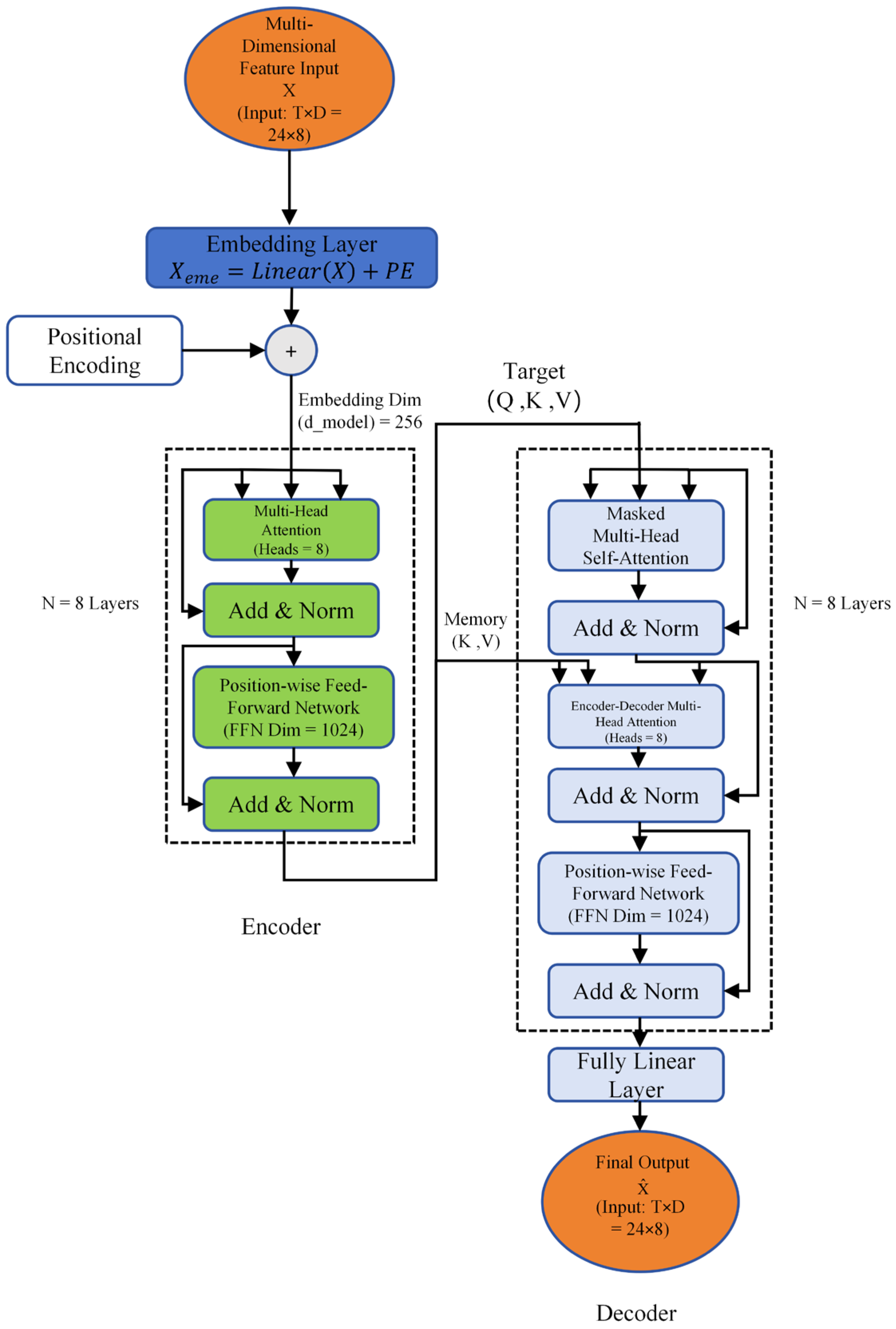
The model’s structural design aligns with the conventional Transformer autoencoder architecture, encompassing an encoder and a decoder [21]. The workflow can be conceptualized as a process of “reading comprehension” and “precise retelling”: the encoder processes the input time series and compresses it into a condensed latent representation, while the decoder attempts to reconstruct the original sequence from this latent representation. The representation of an input time series is as follows:
X T × D
T is imperative to ascertain the time step and D = 8 is the feature dimension at each time point. Figure 3 illustrates the Transformer autoencoder structure.
The model’s processing flow:
  • Input Embedding and Positional Encoding;
The Transformer model doesn’t perceive order, so positional information must be injected into the input data. To provide a richer expressive space, we map the original features to a higher-dimensional model space ( d m o d e l ).
X emb = Linear ( X ) + P pos
In this context, where Linear ( X ) denotes a linear layer that elevates each time step’s D -dimensional feature vector to d m o d e l dimensions. P pos is a fixed position encoding matrix that provides unique timestamp information for each time step. This enables the model to understand the sequence’s temporal order and relative positions.
2.
Encoder;
The encoder’s role is to develop a deep understanding of the complex relationships within the input sequence.
Z e n c o d e d = Encoder ( X e m b )
It consists of N identical encoder layers stacked on top of each other. Each layer contains multi-head self-attention and a feedforward neural network. After the N layers are stacked, the encoder ultimately produces an output containing contextual information Z e n c o d e d .
3.
Decoder;
The decoder’s job is to use the output from the encoder, Z e n c o d e d , to recreate the original input sequence as precisely as possible.
X p r e d = Linear ( Decoder Z e n c o d e d )
It is composed of N decoder layers stacked together. The structure is similar to the encoder layers, but it has an additional “encoder–decoder attention” module. This allows the decoder to extract the most helpful information from Z e n c o d e d for the current task at each step of the reconstruction process.
4.
Differential Feature Extraction;
This paper uses multiple dimensions to form a set of highly structured features. These features are measures of “anomaly,” providing a foundation for intelligent decision-making.
(1)
Global Reconstruction Error Features;
These features provide a macro-level measurement of the model reconstruction process’s overall fidelity.
Mean Squared Error (MSE) is a compact, low-dimensional manifold that models learn to represent “normal” surface dynamics. Any data that does not conform to this learned normal pattern (such as fire points) will be difficult for the model to reconstruct accurately, resulting in a large, quantifiable reconstruction error.
L recon = 1 T D t = 1 T d = 1 D ( x t , d x ^ t , d ) 2
In this context, x t , d denotes the dth feature value of the original input sequence X at time step t, while x ^ t , d signifies the corresponding value of the model-reconstructed sequence T D at the same position. The model calculates the square of the difference between the original sequence and the reconstructed sequence at each dimension and each time point. Then, all these differences are summed and divided by the total number of points ( T D ) to obtain the average.
The mean absolute error (MAE) is a supplement to the mean square error (MSE) in that it is less sensitive to extreme outliers.
L mae _ recon = 1 T D t = 1 T d = 1 D x t , d x ^ t , d
(2)
Time-Dimension Error Features;
The following features are indicative of the distribution pattern of reconstruction errors in the time dimension.
Firstly, the calculation of the Euclidean distance error, e t , at each time point, t , is required in order to obtain an error vector, E , defined as follows: E = e 1 , e 2 , …… e T .
e t = X actual , t X pred , t 2
X actual , t and X pred , t are the original and reconstructed 8-dimensional feature vectors at time. e t is a measure of reconstruction failure at time. The paper extracts four key statistical features based on this error vector.
  • Mean Error ( r e c o n m e a n );
r e c o n m e a n = 1 T t = 1 T e t
This is the arithmetic mean of the error vector, reflecting the average difficulty of model reconstruction across the entire time window. A continuously burning fire point or a severely occluded signal can cause a high error.
  • Standard Deviation of Error ( r e c o n s t d );
r e c o n s t d = 1 T 1 t = 1 T ( e t r e c o n _ t s _ m e a n ) 2
This feature measures the volatility, or instability, of the error sequence. A sudden, early fire point may produce large errors at only one or two time points while errors are minimal at other time points. Such substantial alterations invariably give rise to elevated levels of standard deviation.
  • Skewness of the Reconstruction Error ( r e c o n s k e w );
r e c o n s k e w = 1 T t = 1 T ( e t r e c o n m e a n ) 3 1 T t = 1 T ( e t r e c o n m e a n ) 2 3 / 2
In typical circumstances, reconstruction errors typically exhibit a symmetrical distribution (e.g., a Gaussian distribution), with skewness values approximating 0. Nevertheless, the occurrence of fire points ordinarily manifests as elevated error values at specific time points, thereby forming a protracted “right tail” and consequently giving rise to a considerably skewed error distribution.
  • Kurtosis of the Reconstruction Error ( r e c o n k u r t );
r e c o n k u r t = 1 T t = 1 T ( e t r e c o n m e a n ) 4 1 T t = 1 T ( e t r e c o n m e a n ) 2 2
The kurtosis is a measure of the sharpness of the error distribution. An analysis of the kurtosis values indicates that the reconstruction errors are primarily concentrated in a few intense, far-out “peaks,” which is a typical characteristic of hotspot signals.
(3)
Latent Space Features;
These features quantify the extent to which the input sequence deviates from “normal” patterns in the abstract feature space learned by the model.
Firstly, the encoder’s understanding of the entire time series, i.e., the output tensor, is aggregated by taking the average over the time dimension. This results in a single latent space vector z s a m p l e that represents the entire sequence.
z s a m p l e = 1 T t = 1 T Z e n c o d e d , t
It is evident that the z s a m p l e is a holistic and comprehensive representation of the entire input time series. The focus has shifted from the analysis of specific moments to the examination of the macro-level characteristics of entire events. To establish a baseline for the measurement of ‘normal’ behavior, it is first necessary to pre-compute an average latent space vector across the entirety of the training data without fire points. We then define this vector as the centroid of the ‘normal’ pattern z c e n t r o i d .
z c e n t r o i d = 1 N i = 1 N E n c o d e r ( E m b e d d i n g ( X n o r m a l ( i ) ) )
For the sake of clarity, the dataset represented by X n o r m a l ( i ) in (23) is identical to the entire “fire-free” dataset that was utilized for the self-supervised training of the Transformer autoencoder.
This guarantees that the centroid accurately represents the central tendency of all normal surface dynamics learned by the model. This quantity can be regarded as the “average state” of all normal surface dynamics that the model has learned. In the subsequent stage of the process, the latent space distance, l a t e n t e u c l i d e a n , is calculated. This metric is of the utmost importance in this particular feature group. The Euclidean distance between the latent space vector of the current sample and the “normal centroid” is calculated directly.
l a t e n t e u c l i d e a n = z s a m p l e z c e n t r o i d 2
A small distance value shows the sample’s current high similarity to the “standard normal sample” in terms of deep semantics. A large value indicates an anomaly, showing that even if the model’s reconstruction error is low, the sample is different from normal patterns.
Additionally, this paper analyses the statistical characteristics of sample latent space vectors z s a m p l e  to provide more auxiliary information.

3.3. Semi-Supervised Hotspot Detection Based on XGBoost

3.3.1. Design Concept

The initial stage of this process yields a high-dimensional, information-rich feature space, comprising reconstruction errors and latent space distances. While it provides abundant discriminative information, it also presents more advanced decision-making challenges. In this abstract feature space, the boundary between fire and non-fire is highly complex and nonlinear. Decision-making methods based on fixed, manually defined thresholds are inadequate, as they attempt to partition this high-dimensional space with a simple hyperplane, which cannot adapt to the complex interrelationships between features.
To address this issue, a hybrid model combining “deep learning feature extraction + traditional machine learning classifiers” is adopted. The approach under discussion here makes use of deep learning’s automatic representation learning in order to map complex data into a structured, discriminative feature space. Next, we use classical machine learning classifiers to make efficient and interpretable decisions.
The final decision engine is XGBoost (eXtreme Gradient Boosting). The integration of decision trees within the XGBoost framework facilitates the learning of complex nonlinear decision boundaries [22], thereby addressing the “complex feature space decision-making dilemma.” Furthermore, XGBoost demonstrates a high level of proficiency in the management of structured tabular data [23], exhibiting a precise alignment with the format of the deep feature vectors generated during the initial stage.

3.3.2. XGBoost Model

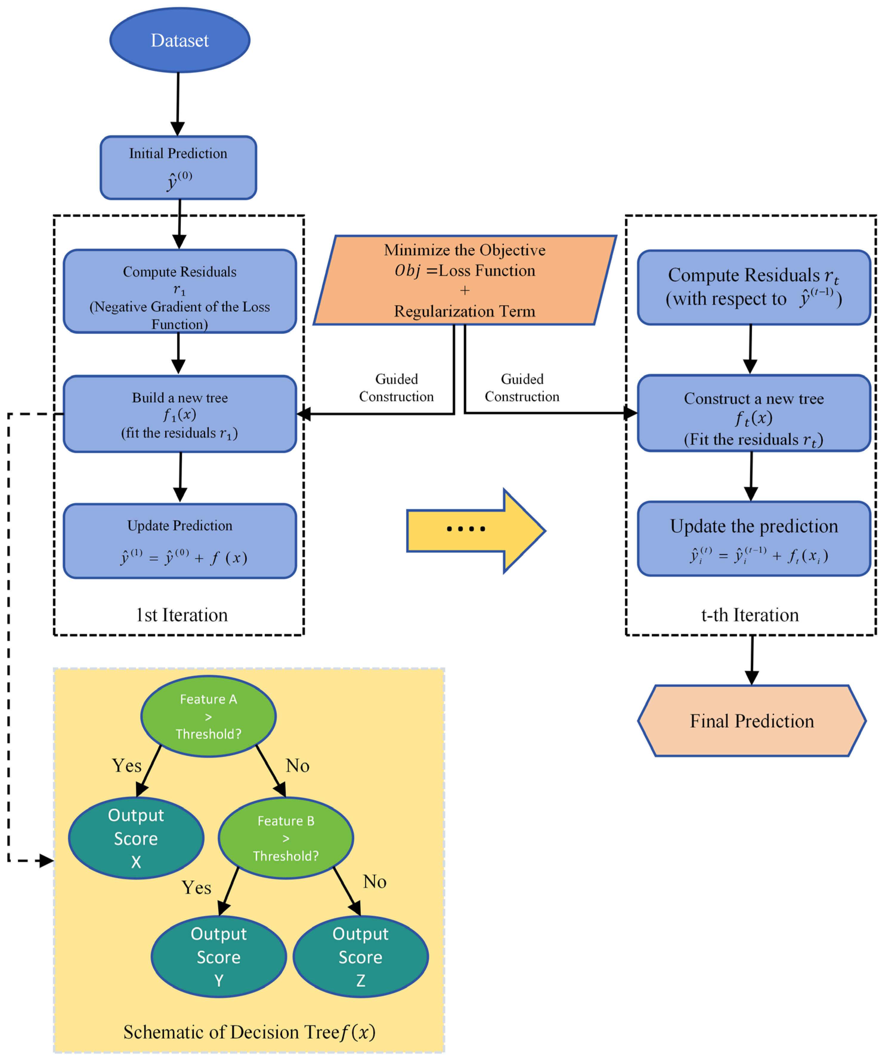
XGBoost is an efficient and scalable implementation based on the gradient boosting framework. The ensemble model under discussion is not a single model, but rather an ensemble of weak learners (typically decision trees) that are iteratively trained and combined into a strong learner for final prediction, as illustrated in Figure 4.
The fundamental principle underpinning this approach is the concept of additive training. The algorithm constructs the model in a forward distribution manner, adding a new decision tree in each iteration to fit the negative gradient of the loss function from the previous iteration’s prediction. The following equation represents the prediction value at the t -th iteration, y ^ i ( t ) , for the i -th sample:
y ^ i ( t ) = y ^ i ( t 1 ) + f t ( x i )
In this study, y ^ i ( t ) denotes the prediction result of the previous t 1 trees on sample x i . f t x i is the prediction value of the decision tree learned in the t ( t h ) iteration of the sample x i (i.e., the score of a leaf node). The superior performance of XGBoost is attributable to its innovative objective function design. In the t ( t h ) iteration, the objective function   O b j ( t ) for model optimization comprises two elements: the loss function and the regularization term.
O b j ( t ) = i = 1 n l ( y i , y ^ i ( t 1 ) + f t ( x i ) ) + Ω ( f t )
In this context, l y i , 🞄 denotes a differentiable loss function that quantifies the discrepancy between the true labels y i and the predicted values. In the context of binary classification problems, the logistic loss is conventionally employed.
Ω ( f t ) functions as a regularization penalty term, effectively mitigating the complexity of the tree-based models (i.e., t -trees f t ). This mechanism is instrumental in averting the phenomenon of overfitting in XGBoost models. The term is defined as follows:
Ω ( f ) = γ T + 1 2 λ j = 1 T w j 2
In the context of a decision tree, γ denotes the number of leaf nodes, w j represents the weight (or score) of the j -th leaf node, and γ and λ are hyperparameters that regulate the intensity of regularisation. This penalty term functions to suppress the model from generating overly complex trees (i.e., trees with too many leaf nodes) and leaf nodes with overly large weights. The effect of this is to encourage the model to learn simpler and more generalisable decision rules.
The algorithm performs the second-order Taylor expansion and optimizes the objective function with the regularisation term. These two processes enable XGBoost to efficiently identify the optimal decision tree to add at each step f t . The ability to exercise direct control over model complexity, in conjunction with a highly optimised engineering implementation, enables XGBoost to attain remarkable performance and robustness when processing the structured deep features generated during the initial stage.

3.3.3. Iterative Pseudo-Label Self-Training

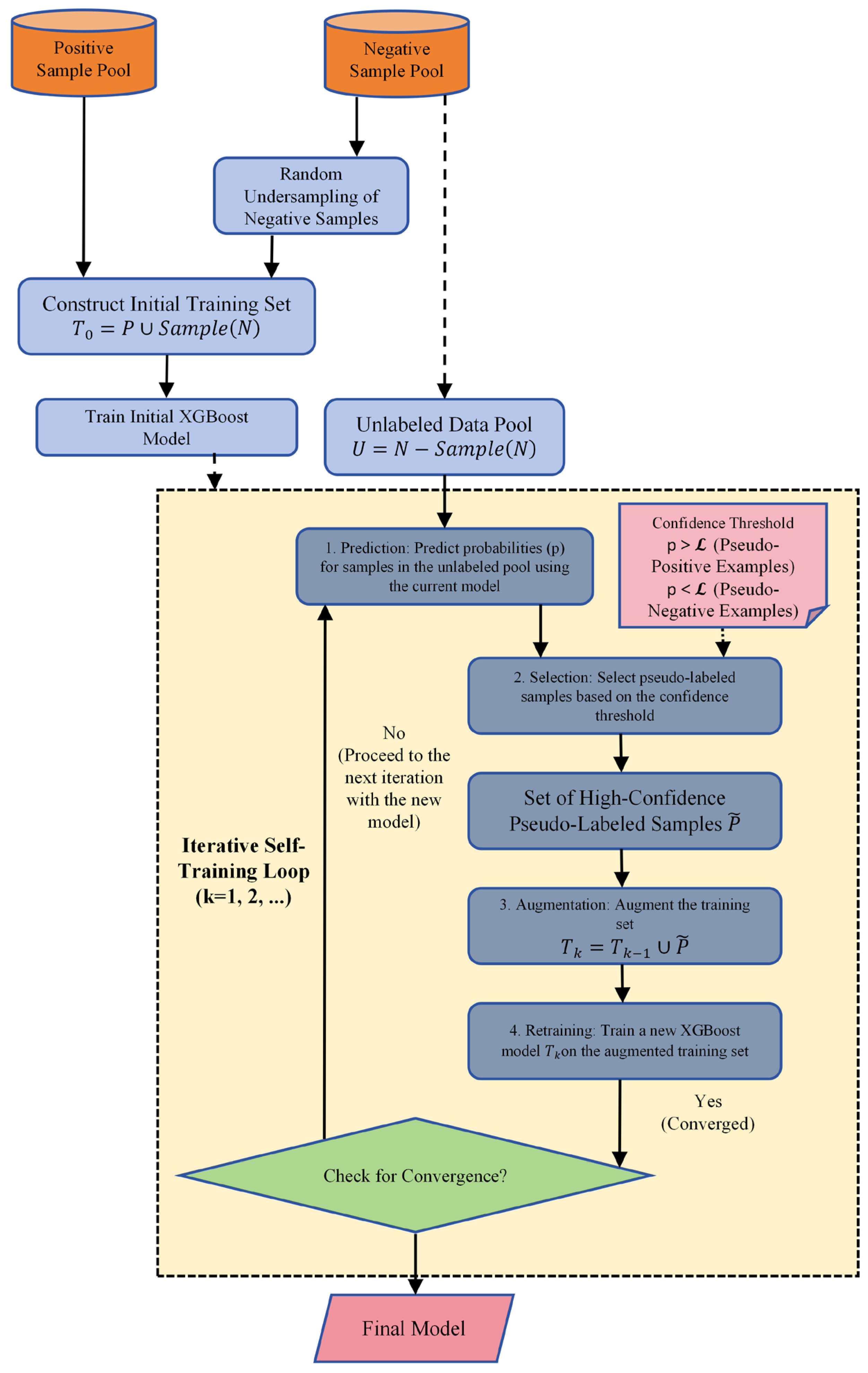
The proposed methodology is an iterative pseudo-label self-training process [24], which efficiently leverages large-scale data and continuously optimises the model’s decision boundaries through a positive, self-reinforcing feedback loop. Instead of utilising all the data concurrently, the process employs a curriculum learning approach, whereby the model initially learns from the easiest-to-distinguish unlabelled samples and subsequently progresses to more “ambiguous” boundary data as it acquires new knowledge.
The training strategy comprises four steps to ensure full utilization of unlabelled data while minimizing confirmation bias [25]—the risk of amplifying and solidifying early incorrect predictions. Figure 5 illustrates the architectural design.
1.
Training set construction;
The training process commences with a processed initial dataset (   D i n i t i a l ), which comprises two constituent parts.
Positive sample set ( P ): The database contains all samples that have been verified by human experts as known fire points. This constitutes the basis for the model to learn fire point features.
The term ‘reliable negative sample set’ ( R N ) is employed to denote a set of data that has been proven to be unreliable. This constitutes a pivotal innovation of the present paper. In lieu of the arbitrary selection of non-fire point samples, there is instead the intelligent leveraging of the results from the initial phase. Specifically, all data were entered into the pre-trained Transformer autoencoder, and samples with extremely low reconstruction error (the bottom 5% of the error distribution) were filtered out. Pursuant to an initial automated filtration of samples exhibiting the lowest reconstruction error (bottom 5%), a concluding manual screening was executed as a quality control measure to ascertain the purity of the RN set. The verification process was executed in two stages. Candidates are to be inspected for visual anomalies using multi-spectral time-series data. Such anomalies may include, but are not limited to, the presence of faint smoke or the development of burn scars. Furthermore, spatio-temporal cross-validation against established fire products, such as JAXA WLF and MCD14ML, is performed to reject any candidates near a known fire. While this manual check was employed in this study to guarantee a high-purity initial training set, it is acknowledged that a fully automated process is preferable for reproducibility. This step can be automated in the future by a rule-based filter that automatically rejects candidates based on momentary spikes in key anomaly features or their proximity to other confirmed fire detections. Following a manual screening process, these samples can be considered “normal” with a high degree of confidence and are designated as 0, thereby forming a reliable negative sample set. The initial training set, designated D , is constructed as follows: D i n i t i a l = P R N . Subsequently, all remaining samples are classified into a large unlabelled data pool ( U ).
2.
Training and handling imbalance;
The initial training set   D i n i t i a l is utilised in the training of the primary baseline XGBoost model, designated M 0 . In light of the rarity of events pertaining to fire points, even after screening, the number of reliable negative samples is ordinarily considerably larger than that of positive samples, thus giving rise to a marked imbalance in the classes. To address this issue, it is necessary to set the key XGBoost parameter s c a l e _ p o s _ w e i g h t during the training process.
s c a l e _ p o s _ w e i g h t = c o u n t ( N e g a t i v e   S a m p l e s ) c o u n t ( P o s i t i v e   S a m p l e s ) = | R N | | P |
The parameter is set to the ratio of negative to positive samples. In the loss function, it assigns greater weight to scarce positive samples (fires), thereby preventing the model from exhibiting a bias towards the majority negative class. This ensures that the model learns balanced representations for both positive and negative samples.
3.
Iterative enhancement loop;
After obtaining the baseline model M 0 , we begin the iterative self-training process. This process repeats k times until the model achieves convergence.
(1)
Predict;
The employment of the prevailing mode M k is requisite in order to predict all samples contained within the unlabelled data pool U k , thereby ascertaining the probability that each sample x i U k is predicted as a fire:
p i = P y = 1 x i ; M k
(2)
Filter;
This is the fundamental step in the process of suppressing confirmation bias. The implementation of two strict confidence thresholds, τ p o s and   τ n e g (in this paper, τ p o s   = 0.98 and   τ n e g   = 0.02 ), enables the filtration of the model’s “most confident” prediction results from the unlabelled pool.
  • Filtering pseudo-positive samples ( P p s e u d o )
    P p s e u d o = { ( x i , 1 ) | x i U k , p i > τ p o s }
  • Filtering pseudo-negative samples ( N p s e u d o )
    N p s e u d o = { ( x i , 0 ) | x i U k , p i < τ n e g }
By exclusively accepting high-confidence pseudo-labels, this approach ensures that newly incorporated training samples maintain a superior quality standard. This strategy, in turn, prevents any discernible deterioration in model performance that noisy labels might cause.
(3)
Augmentation;
Add selected samples to the training set and remove them from the unlabeled pool.
D k + 1 = D k P p s e u d o N p s e u d o U k + 1 = U k ( P p s e u d o N p s e u d o )
(4)
Retrain;
The augmented training set D k + 1 should be used to recalculate the parameters s c a l e _ p o s _ w e i g h t , and a more robust XGBoost model M k + 1 should be trained.
4.
Convergence and Final Optimization
The iterative process is repeated until there is no significant improvement in performance on an independent hold-out validation set, or until a predetermined maximum number of iterations is reached, at which point convergence is indicated. In conclusion, the augmented training set (true labels + high-confidence pseudo-labels) is employed to perform systematic hyperparameter optimisation of XGBoost via a cross-validated Optuna search, thereby yielding the final classifier.

4. Experimental Results and Analysis

4.1. Experimental Setup

The experimental approach involves the utilisation of Himawari-8/9 observations over Yunnan, in conjunction with fire-point labels provided by the Yunnan Electric Power Research Institute (Southern Power Grid). The evaluation process utilises standard fire-detection metrics:
1.
Precision;
Precision is defined as the proportion of samples correctly predicted as fire points among all samples predicted as fire points by the model. The primary focus of this study is to ascertain the accuracy of the model’s predictions.
P r e c i s i o n = T P T P + F P
2.
Recall;
Recall measures the proportion of true fire points detected by the model. It focuses on the model’s ability to detect true fire points.
R e c a l l = T P T P + F N
9.
F 1 Score;
The F 1 score is defined as the harmonic mean of precision and recall, serving as a pivotal metric for the comprehensive evaluation of model performance. When both precision and recall are high, the F 1 score is also high.
F 1 = 2 × p r e c i s i o n × r e c a l l p r e c i s i o n + r e c a l l

4.2. Experimental Environment

4.2.1. Environment Configuration

CPU: 16 vCPU Intel(R) Xeon(R) Platinum 8358P; GPU: NVIDIA GeForce RTX 4090 (24 GB VRAM); Memory: 120 GB; Operating System: Ubuntu 20.04 LTS; Core Framework: PyTorch 2.3.0; CUDA: 12.1; Python Version: 3.12.

4.2.2. Hyperparameter Settings for the Model

The first-stage Transformer autoencoder utilises input time-series of length 24, embedding dimension 256, multi-head attention with 8 heads, 8 encoder and 8 decoder layers, and a feedforward dimension of 1024. The dropout rate is 0.1. The optimization process utilises the AdamW algorithm with an initial learning rate of 3 × 10⁻⁴, a cosine-annealing scheduler with a period of 30, and a weight decay parameter of 1 × 10⁻⁵. The training process utilises a batch size of 128, gradient accumulation set to 2, and an epoch count of 500. The loss function employed is the mean square error (MSE) loss. The early stopping process uses a patience value of 50 and a minimum delta value of 1 × 10⁻⁶. The gradient clipping threshold has been set to 0.5.
The second stage of the process involves the implementation of a semi-supervised XGBoost classifier. The initial negative-to-positive ratio is 10:1, with a maximum initial negative-sample cap of 5000. The pseudo-label filtering thresholds are as follows: positive > 0.985, negative < 0.015. The self-training loop is capable of up to three iterations; early stopping is employed if patience = 3 (no significant improvement), and the minimum F1 improvement to continue is >0.005. The calculation of class imbalance weight is derived from the class ratios of each training set.
Hyperparameter optimization is performed with Optuna (Bayesian search). The experiment was conducted across a total of 50 trials, with each trial being performed five times to ensure the reliability and precision of the results. The search ranges are as follows: n_trees: [50, 300]; max_depth: [3, 8]; learning_rate: [0.01, 0.2]; colsample: [0.7, 1.0]; subsample: [0.7, 1.0]; min_split_gain: [0, 0.5]; reg_alpha (L1): [0.01, 1.0]; and reg_lambda (L2): [0.01, 1.0]

4.3. Experimental Results

4.3.1. Case Analysis

To provide a comprehensive evaluation of the effectiveness and robustness of the proposed framework in real-world scenarios, four representative fire events were analysed. The study encompassed both human-initiated controlled burns and wildfires that occurred spontaneously under diverse land cover types, including grasslands, agroforestry transition zones, and mountainous forests. This comprehensive approach facilitated a meticulous evaluation of the model’s performance.
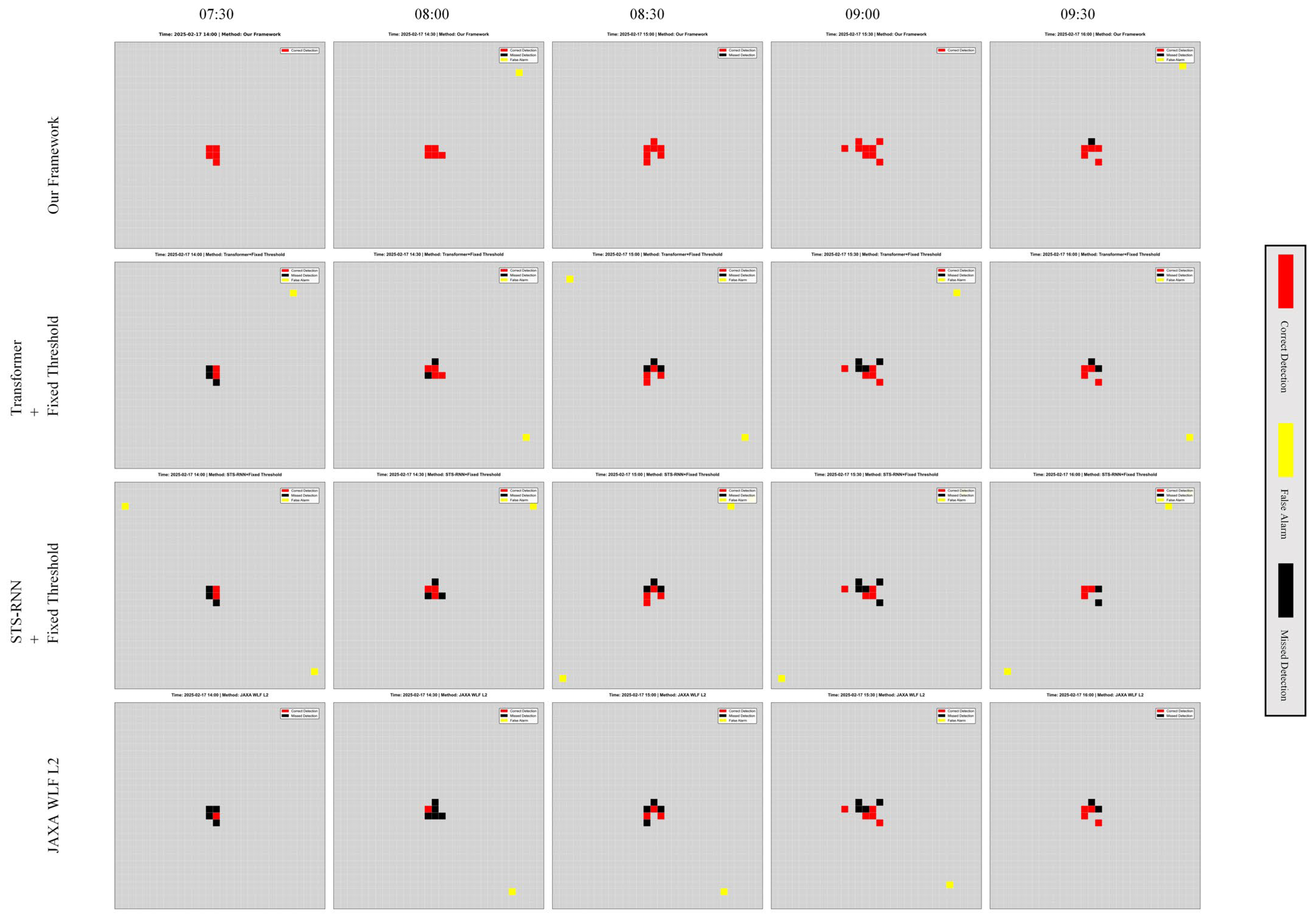
The initial incident (Case 1) transpired at a designated burn location in Gongguoqiao Town, Yunlong County, Dali City, Yunnan Province, China (99.2° E, 25.8° N) on 17 January 2025, from 07:30 to 09:30 UTC, as illustrated in Figure 6a. The occurrence was corroborated through the utilisation of the Yunnan Power Grid Tianwang System and field inspections, thereby substantiating its authenticity. The case featured a limited burn scale, weak thermal signals, and a short duration, which posed a significant challenge to the algorithm’s detection sensitivity.
Case 2 pertains to a grassland wildfire that occurred in Kaiyuan City, Honghe Hani and Yi Autonomous Prefecture, Yunnan Province, China (103.1° E, 23.8° N) on 27 February 2025, between 14:00 and 16:00 UTC, as illustrated in Figure 6b. The event was confirmed to be genuine through a combination of automated verification by the Yunnan Power Grid’s Tianwang System and manual inspections. In contrast to the limited and smoke-free combustion observed in Case 1, this incident manifested pronounced flames and discernible smoke plumes. Aerosol absorption and subsequent scattering of thermal radiation resulted in significant signal attenuation, while dynamic smoke plumes introduced complex background interference. The present case study aims to evaluate the robustness of the framework under conditions of severe aerosol pollution and signal attenuation.
Case 3 pertains to an agricultural–forest wildfire that occurred in Milixiang Township, Yuanjiang County, Yuxi City, Yunnan Province, China (101.9° E, 23.5° N) on 17 February 2025, between 08:30 and 11:30 UTC, as illustrated in Figure 6c. The event was confirmed as genuine through a combination of automated verification using the Yunnan Power Grid’s Tianwang System and manual inspections. The site is located at the intersection of farmland, forest, and villages, exhibiting highly variable surface thermodynamic properties. Crops, diverse tree species, and artificial structures exhibit distinct temperature responses under solar radiation, thereby imposing greater demands on the algorithm’s discrimination ability. The present case study aims to evaluate the model’s accuracy in separating true fire points from “thermal background” noise under complex surface conditions.
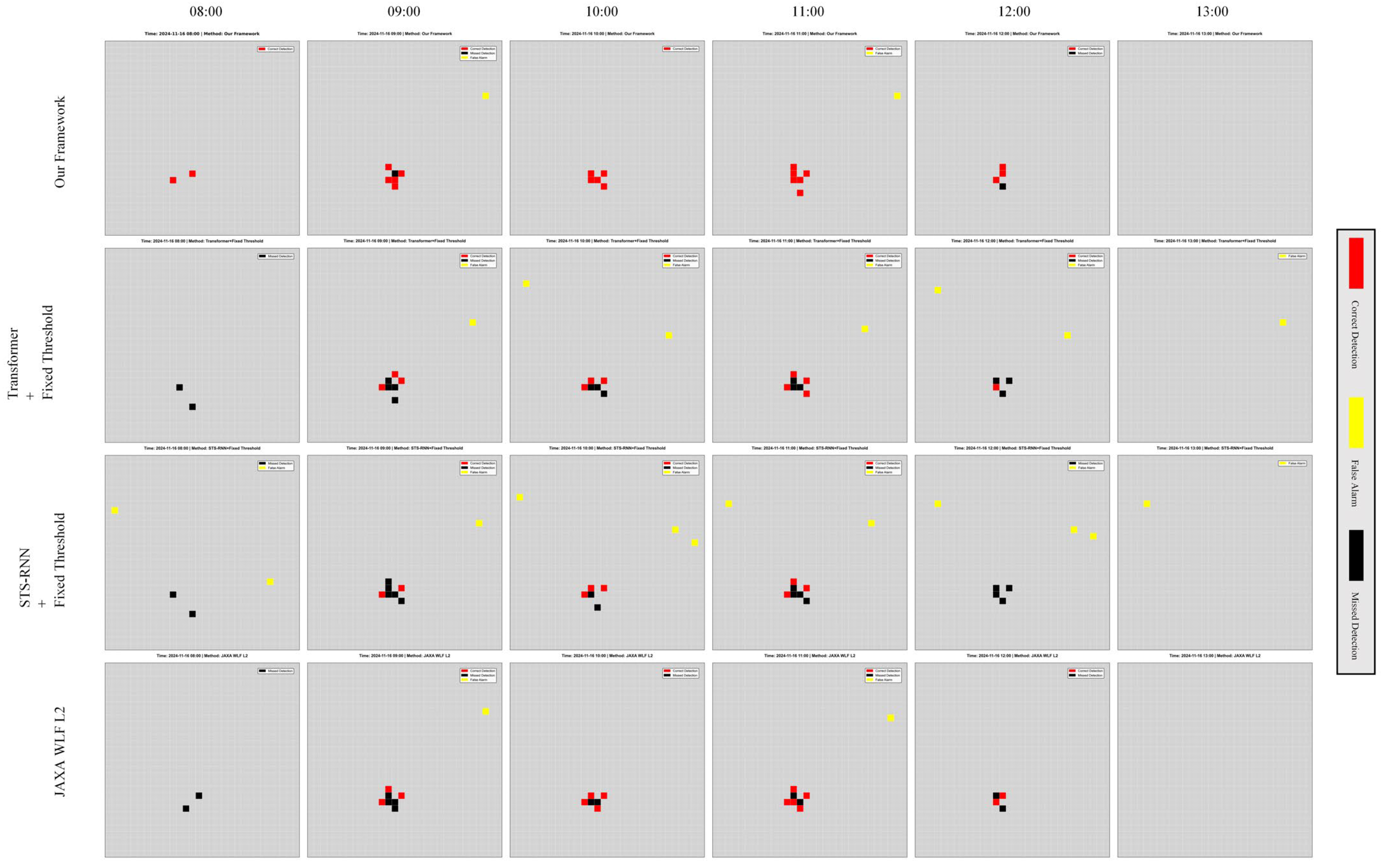
Case 4 is a mountain forest fire in Minle Town, Jinggu County, Puer City, Yunnan Province, China (100.4° E, 23.5° N), which occurred from 08:00–12:00 UTC on 16 November 2024, as illustrated in Figure 6d. The authenticity of the event was confirmed through a combination of automated verification by the Yunnan Power Grid’s Tianwang System and manual inspections. The topography of the site is characterised by rugged terrain, dense forest cover, rapid fire spread, and intense flames. The contrast between sunlit and shaded slopes leads to significant spatial heterogeneity in surface temperatures. Furthermore, dense canopies have the capacity to obscure heat signals. The present case study aims to evaluate the model’s capacity to dynamically monitor and accurately characterise high-intensity fires under complex terrain and heavy vegetation cover.

4.3.2. Quantitative Performance Comparison

To perform an objective and quantitative assessment of performance, this study compares the proposed framework with three baselines across the four representative cases. The baselines include: The following three cases are considered: An RNN with fixed-threshold decision (RNN + Fixed Threshold); the proposed Transformer encoder with fixed-threshold decision (Transformer + Fixed Threshold), isolating the effect of the decision mechanism; and the official Himawari-8/9 fire product (JAXA WLF L2) released by JAXA, serving as an operational benchmark. As illustrated in Table 3, precision, recall and F1 score are demonstrated for each model across the four cases.
The proposed framework yielded substantially superior F1 scores across the four cases (macro-average 0.8880, micro-average 0.8839), indicating a superior balance between precision and recall. The commercial JAXA WLF L2 product attains higher precision in some cases (average 0.8771), but at the cost of severe under-detection (average recall 0.2937), producing low overall F1 and limiting its utility for early, comprehensive monitoring. The temporal feature extractor, upgraded from RNN to Transformer, has been shown to systematically improve discriminative power (mean F1 ≈ 0.44 → 0.57). This is attributable to the self-attention mechanism’s ability to capture long-range dependencies in time series. It is crucial to note that replacing a fixed-threshold decision with an XGBoost classifier on the same Transformer features results in a substantial increase in the average F1 score, from ≈0.57 to >0.88. This substantial enhancement underscores the significance of simple thresholding in high-dimensional, nonlinear feature spaces generated by Transformer models. In contrast, XGBoost employs an adaptive learning approach to delineate intricate decision boundaries, thereby facilitating a notable enhancement in detection performance.

4.3.3. Qualitative Results Visualization

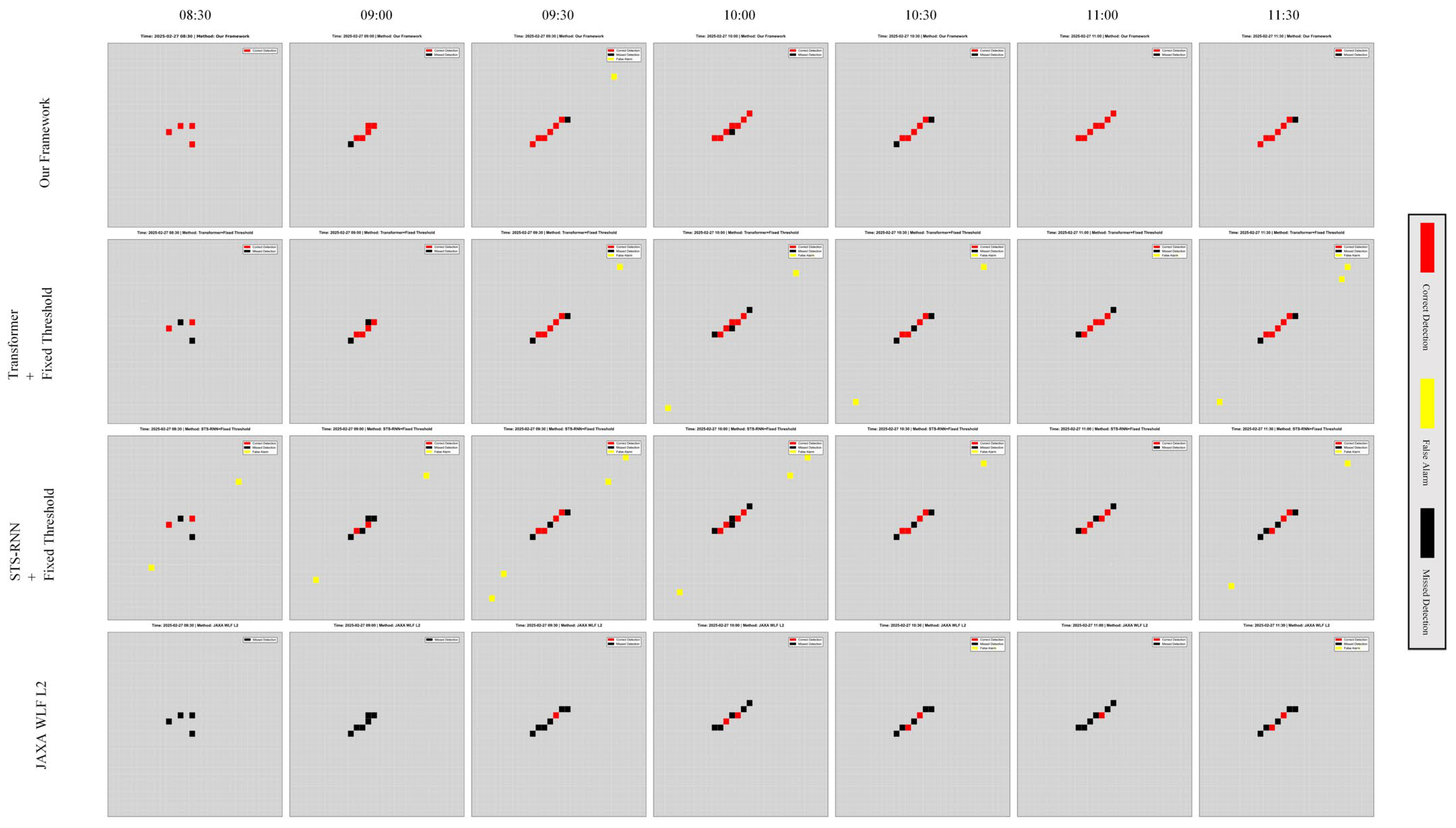
To facilitate a comparison of the manner in which models reconstruct spatiotemporal fire dynamics, the present study employs a visualisation technique that utilises pixel-wise detection results over time for four illustrative cases. The figures demonstrate the temporal evolution of four methods: the proposed framework, Transformer + fixed threshold, RNN + fixed threshold, and JAXA WLF L2. These visualisations facilitate a qualitative comparison of detection sensitivity, false alarms and temporal consistency.
  • Legend:
  • Red: correctly detected fire points (True Positive, TP);
  • Black: missed true fire points (False Negative, FN);
  • Yellow: false alarms (False Positive, FP).
A thorough evaluation of the visualisation outcomes reveals a consistent pattern across all cases: the proposed framework demonstrates superiority over all baselines in terms of spatial continuity and temporal persistence of detected fire points. In both low-intensity planned burns (Figure 7) and high-intensity mountain fires (Figure 10), the framework produces dense TP clusters that closely follow the macro-scale morphology and evolution of the fire field.
In contrast, the baselines—inclusive of the operational JAXA product—demonstrate a “spotty” detection pattern with a multitude of false negatives and fragmented spatial distributions, indicating a propensity to identify isolated peaks as opposed to the complete contour and development trend of the fire scene. The visualisations also corroborate the findings from the ablation study: replacing RNN with Transformer generally increases TP density (second row vs. third row), but the largest gain occurs when the fixed-threshold decision is replaced by the proposed decision mechanism (first row vs. second row). This finding suggests that, while enhanced temporal features are valuable, the primary bottleneck in high-dimensional feature spaces is the decision rule. The utilisation of a data-driven classifier is necessary to fully exploit Transformer features and achieve substantial detection improvements.

4.3.4. Error Analysis

While the proposed framework demonstrates superior overall performance, a detailed analysis of the remaining false negatives (FN) and false positives (FP) is crucial for understanding the model’s limitations and guiding future improvements. The following error patterns are identified by our analysis, which is based on the visualization results in Figure 7, Figure 8, Figure 9 and Figure 10:
1.
Analysis of False Negatives (FN);
False negatives, or missed fire detections (represented by black points in the visualizations), primarily occurred under two conditions:
Weak Initial Signals: In several cases, particularly during the nascent stages of a low-intensity fire like the human-planned controlled burning (Case 1), the model occasionally failed to detect the fire in the very first time step. This phenomenon can be attributed to the fact that the initial thermal anomaly was too subtle to be reliably distinguished from background thermal noise by the engineered feature set.
Signal Obscuration: In scenarios characterized by substantial smoke, such as the grassland wildfire (Case 2) and the mountain forest fire (Case 4), dense smoke plumes could have partially obscured the heat signature from the satellite’s sensor. This signal attenuation is a well-known challenge in the fields of optical and thermal remote sensing. It has been demonstrated that this phenomenon can lead to missed detections, even in the case of active fires.
2.
Analysis of False Positives (FP);
False positives, or false alarms (represented by yellow points), were infrequent but tended to be associated with specific land surface types that can mimic fire signals.
Complex “Thermal Backgrounds”: As evidenced in the agroforestry wildfire (Case 3) and mountain forest fire (Case 4), some FP manifested in regions characterized by intricate and heterogeneous thermodynamic properties. Surfaces such as sunlit barren land, rocky outcrops, or artificial structures can reach high temperatures under direct solar radiation. This phenomenon, known as “thermal background” noise, is occasionally misclassified as a weak fire point despite the implementation of a two-stage filtering approach.
This detailed error analysis suggests that while the model is robust, future work could focus on integrating auxiliary data, such as high-resolution land cover maps, to provide better contextual information and further reduce these types of misclassifications.

4.4. Computational Performance and Near-Real-Time Feasibility

A critical requirement for any operational satellite fire early warning system is the ability to process incoming data in a timely manner. In order to assess the feasibility of our framework for near-real-time deployment, we conducted an analysis of its computational performance in the context of the Himawari-8/9 satellite’s 10-min data revisit cycle.
In principle, the computational complexity of our two-stage model is well-suited for efficient inference. The Transformer’s self-attention mechanism is manageable given the short sequence length (T = 24) used, and the XGBoost classifier is known for its high-speed predictions. Empirically, we benchmarked the performance on our specified hardware (NVIDIA RTX 4090 GPU and Intel Xeon CPU). The total time for the entire pipeline, from the loading of a large regional data tile to the final inference from both the Transformer and XGBoost models, was approximately five to seven minutes. This empirical processing time is substantially less than the 10-min satellite revisit period. This results in a critical margin of 3–5 min, a figure that is indispensable in a real-world operational context. This margin is necessary to account for potential data transfer latencies, I/O bottlenecks, and task queuing. It is noteworthy that this outcome was attained by employing a research-grade implementation, devoid of any production-level code optimization. Consequently, it is reasonable to hypothesize that the processing time could be further reduced in a dedicated operational environment. In summary, the findings of this study demonstrate the computational feasibility of the proposed framework for effective near-real-time implementation as a wildfire early warning system.

5. Conclusions

The proposed two-stage fire detection framework integrates a transformer-based autoencoder for deep feature extraction with a semi-supervised XGBoost model for classification. The primary innovation of this framework is its substitution of the conventional fixed threshold with a data-driven, nonlinear decision-making mechanism. This mechanism enables the precise identification of early and weak fire signals by learning adaptive classification boundaries. In a rigorous validation process involving real fire cases in Yunnan Province, China, the framework attained a consistent F1 score of 0.88, thereby demonstrating a substantial improvement over the official JAXA satellite product and baseline RNN models. The system exhibited noteworthy sensitivity and robustness, particularly in complex scenarios such as small-scale fire points and smoke occlusion.
The primary contribution of this work lies in demonstrating the efficacy of decoupling deep temporal feature learning from a flexible, semi-supervised classification stage. However, we acknowledge its limitations and identify several promising avenues for future research. While the iterative pseudo-labeling strategy has proven to be effective, its performance ceiling remains constrained by the quality of the initial “seed” labels. In order to create a more robust filtering mechanism, future refinements could incorporate uncertainty estimation techniques. Moreover, the present validation is limited to a single, albeit intricate, geographical region. A consequential subsequent step will be to execute exhaustive generalization experiments to assess the model’s efficacy in disparate climatic domains. To provide a more comprehensive context for the evaluation of the framework’s performance, a benchmarking process against other cutting-edge deep learning models is also planned. Consequently, as initially intended, subsequent endeavors will prioritize the incorporation of a more diverse array of observational data to further augment the model’s capacity for generalization.

Author Contributions

Conceptualization, L.D. and Y.W.; methodology, L.D.; software, L.D.; validation, L.D.; formal analysis, L.D.; investigation, L.D. and Y.W.; resources, L.D.; data curation, L.D.; writing—original draft preparation, L.D.; writing—review and editing, L.D. and Y.W.; visualization, L.D.; supervision, Y.W. and C.L.; project administration, L.D., Y.W., W.Z., H.Y. and H.T.; funding acquisition, Y.W. All authors have read and agreed to the published version of the manuscript.

Funding

This research was funded by the science and technology project of China Southern Power Grid Yunnan Power Grid Co., Ltd., grant number. YNKJXM20240241.

Institutional Review Board Statement

Not applicable.

Informed Consent Statement

Not applicable.

Data Availability Statement

The data that support this study were obtained from the Electric Power Research Institute, Yunnan Power Grid Co., Ltd. (China Southern Power Grid) under license. Data are available from the corresponding author upon reasonable request and with permission from the Electric Power Research Institute, Yunnan Power Grid Co., Ltd.

Acknowledgments

We gratefully acknowledge the Electric Power Research Institute, Yunnan Power Grid Co., Ltd. (China Southern Power Grid) for acquiring, processing, and providing the datasets that enabled this research. Their contribution was vital to our analysis and to advancing wildfire detection and prediction using machine learning. The data were provided under license and are available from the corresponding author upon reasonable request and with permission of the data provider.

Conflicts of Interest

Authors Luping Dong, Yifan Wang, Wenjie Zhu, Haixin Yu and Hai Tian were employed by the company Electric Power Research Institute Yunnan Power Grid Co., Ltd. China Southern Power Grid. The remaining authors declare that the research was conducted in the absence of any commercial or financial relationships that could be construed as a potential conflict of interest.

Abbreviations

The following abbreviations are used in this manuscript:
AHIAdvanced Himawari Imager
MODISModerate Resolution Imaging Spectroradiometer
MCD14MLMODIS 1 km Active Fire
JAXA WLF L2JAXA WLF L2 Product
SDSpectral Differences
rTDRobust Temporal Difference
SVSpatial Variance
TBBBrightness Temperature
MIRMid-Infrared
TIRThermal Infrared
SWIRShortwave Infrared
NDFINormalized Difference Fire Index
SEISmoke Extinction Index
SAShortwave Infrared Anomaly
MTRIMultiplicative Thermal-Reflectance Index
TCSTemporal Consistency Score
TransformerTransformer (self-attention network)
XGBoosteXtreme Gradient Boosting
RNNRecurrent Neural Network
GRUGated Recurrent Unit
LSTMLong Short-Term Memory
CNNConvolutional Neural Network
MSEMean Squared Error
MAEMean Absolute Error
TPTrue Positive
FPFalse Positive
FNFalse Negative
PPositive
RNReliable Negative
UUnlabelled

References

  1. Jang, E.; Kang, Y.; Im, J.; Lee, D.-W.; Yoon, J.; Kim, S.-K. Detection and Monitoring of Forest Fires Using Himawari-8 Geostationary Satellite Data in South Korea. Remote Sens. 2019, 11, 271. [Google Scholar] [CrossRef]
  2. Maeda, N.; Tonooka, H. Early Stage Forest Fire Detection from Himawari-8 AHI Images Using a Modified MOD14 Algorithm Combined with Machine Learning. Sensors 2023, 23, 210. [Google Scholar] [CrossRef]
  3. Moreno-Ruiz, J.A.; García-Lázaro, J.R.; Arbelo, M.; Cantón-Garbín, M. MODIS sensor capability to burned area mapping-assessment of performance and improvements provided by the latest standard products in boreal regions. Sensors 2020, 20, 5423. [Google Scholar] [CrossRef] [PubMed]
  4. Ban, Y.; Zhang, P.; Nascetti, A.; Bevington, A.; Wulder, M.A. Near Real-Time Wildfire Progression Monitoring with Sentinel-1 SAR Time Series and Deep Learning. Sci. Rep. 2020, 10, 1322. [Google Scholar] [CrossRef] [PubMed]
  5. Hong, Z.; Tang, Z.; Pan, H.; Zhang, Y.; Zheng, Z.; Zhou, R.; Ma, Z.; Zhang, Y.; Han, Y.; Wang, J.; et al. Active Fire Detection Using a Novel Convolutional Neural Network Based on Himawari-8 Satellite Images. Front. Environ. Sci. 2022, 10, 794028. [Google Scholar] [CrossRef]
  6. Zhang, D.; Huang, C.; Gu, J.; Hou, J.; Zhang, Y.; Han, W.; Dou, P.; Feng, Y. Real-Time Wildfire Detection Algorithm Based on VIIRS Fire Product and Himawari-8 Data. Remote Sens. 2023, 15, 1541. [Google Scholar] [CrossRef]
  7. Hong, D.; Yokoya, N.; Xia, G.S.; Chanussot, J.; Zhu, X.X. X-ModalNet: A semi-supervised deep cross-modal network for classification of remote sensing data. ISPRS J. Photogramm. Remote Sens. 2020, 167, 12–23. [Google Scholar] [CrossRef]
  8. Wang, S.; Chen, W.; Xie, S.M.; Azzari, G.; Lobell, D.B. Weakly Supervised Deep Learning for Segmentation of Remote Sensing Imagery. Remote Sens. 2020, 12, 207. [Google Scholar] [CrossRef]
  9. Moghim, S.; Mehrabi, M. Wildfire assessment using machine learning algorithms in different regions. Fire Ecol. 2024, 20, 104. [Google Scholar] [CrossRef]
  10. Wickramasinghe, C.; Wallace, L.; Reinke, K.; Jones, S. Intercomparison of Himawari-8 AHI-FSA with MODIS and VIIRS active fire products. Int. J. Digit. Earth 2020, 13, 457–473. [Google Scholar] [CrossRef]
  11. Giglio, L.; Schroeder, W.; Justice, C.O. The collection 6 MODIS active fire detection algorithm and fire products. Remote Sens. Environ. 2016, 178, 31–41. [Google Scholar] [CrossRef]
  12. Giglio, L.; Boschetti, L.; Roy, D.P.; Humber, M.L.; Justice, C.O. The Collection 6 MODIS burned area mapping algorithm and product. Remote Sens. Environ. 2018, 217, 72–85. [Google Scholar] [CrossRef]
  13. Windrim, L.; Ramakrishnan, R.; Melkumyan, A.; Murphy, R.J.; Chlingaryan, A. Unsupervised feature-learning for hyperspectral data with autoencoders. Remote Sens. 2019, 11, 864. [Google Scholar] [CrossRef]
  14. Shenoy, J.; Zhang, X.D.; Tao, B.; Mehrotra, S.; Yang, R.; Zhao, H.; Vasisht, D. Self-Supervised Learning across the Spectrum. Remote Sens. 2024, 16, 3470. [Google Scholar] [CrossRef]
  15. Zhou, W.; Shao, Z.; Diao, C.; Cheng, Q. High-resolution remote-sensing imagery retrieval using sparse features by auto-encoder. Remote Sens. Lett. 2015, 6, 775–783. [Google Scholar] [CrossRef]
  16. Ghaderpour, E.; Vujadinovic, T. Change Detection within Remotely Sensed Satellite Image Time Series via Spectral Analysis. Remote Sens. 2020, 12, 4001. [Google Scholar] [CrossRef]
  17. Hanson, G.; Schmidt, C.C.; Lindstrom, S.J.; Lovellette, A.M.; Wood, C.; Weidner, S. Multispectral Satellite Imagery Products for Fire Weather Applications. J. Atmos. Ocean. Technol. 2023, 40, 881–899. [Google Scholar]
  18. Gentilucci, M.; Younes, H.; Hadji, R.; Casagli, N.; Pambianchi, G. Influence of land surface temperatures, precipitation, total water storage anomaly and fraction of absorbed photosynthetically active radiation anomaly, obtained from MODIS, IMERG and GRACE satellite products on wildfires in eastern Central Italy. Int. J. Remote Sens. 2025, 46, 5465–5499. [Google Scholar]
  19. Yuan, Y.; Lin, L. Self-supervised pretraining of transformers for satellite image time series classification. IEEE J. Sel. Top. Appl. Earth Obs. Remote Sens. 2021, 14, 474–487. [Google Scholar] [CrossRef]
  20. Yang, J.; Wan, H.; Shang, Z. Enhanced hybrid CNN and transformer network for remote sensing image change detection. Sci. Rep. 2025, 15, 10161. [Google Scholar] [CrossRef]
  21. Wang, R.; Ma, L.; He, G.; Johnson, B.A.; Yan, Z.; Chang, M.; Liang, Y. Transformers for Remote Sensing: A Systematic Review and Analysis. Sensors 2024, 24, 3495. [Google Scholar] [CrossRef]
  22. Haque, A.; Soliman, H. A Transformer-Based Autoencoder with Isolation Forest and XGBoost for Malfunction and Intrusion Detection in Wireless Sensor Networks for Forest Fire Prediction. Future Internet 2025, 17, 164. [Google Scholar] [CrossRef]
  23. Zhang, H.; Eziz, A.; Xiao, J.; Tao, S.; Wang, S.; Tang, Z.; Zhu, J.; Fang, J. High-Resolution Vegetation Mapping Using eXtreme Gradient Boosting Based on Extensive Features. Remote Sens. 2019, 11, 1505. [Google Scholar] [CrossRef]
  24. Shadrin, D.; Illarionova, S.; Gubanov, F.; Evteeva, K.; Mironenko, M.; Levchunets, I.; Belousov, R.; Burnaev, E. Wildfire spreading prediction using multimodal data and deep neural network approach. Sci. Rep. 2024, 14, 2606. [Google Scholar] [CrossRef]
  25. Chen, Y.; Yang, Z.; Zhang, L.; Cai, W. A semi-supervised boundary segmentation network for remote sensing images. Sci. Rep. 2025, 15, 2007. [Google Scholar] [CrossRef]
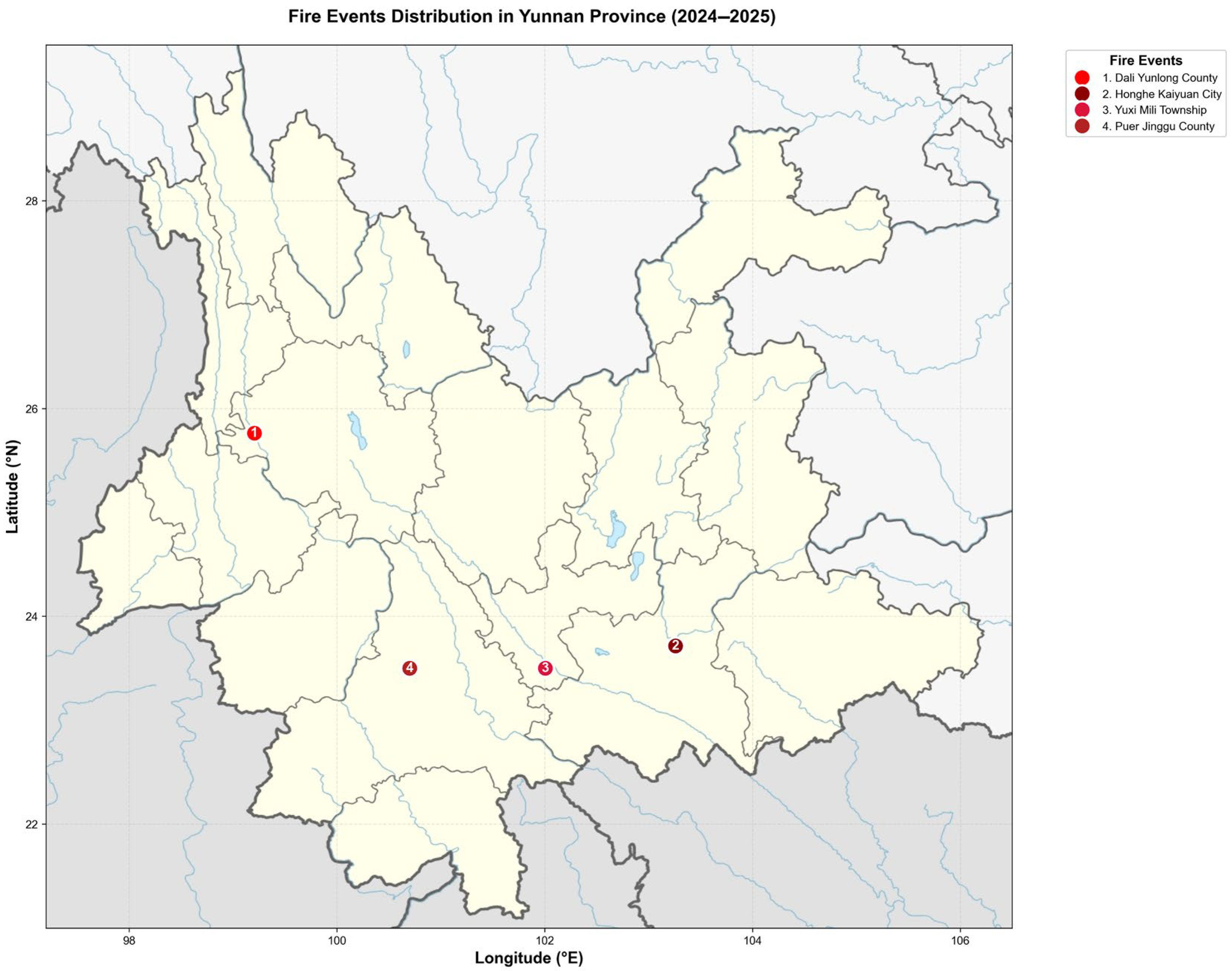
Figure 1. Study area and geographical locations of four representative fire events used for case analysis.
Fire 08 00376 g001
Figure 2. Overall architecture diagram of the fire point detection framework based on Transformer and XGBoost.
Fire 08 00376 g002
Figure 3. Transformer autoencoder network structure.
Fire 08 00376 g003
Figure 4. XGBoost ensemble learning architecture diagram.
Fire 08 00376 g004
Figure 5. Diagram of pseudo-label self-training workflow.
Fire 08 00376 g005
Figure 6. Four representative fire events and their surface environments: (a) Scheduled burn points; (b) Grassland wildfires; (c) Agricultural and forest wildfires; (d) Mountain forest wildfires.
Fire 08 00376 g006
Figure 7. Spatio-temporal visualization comparison of fire point detection results for Case 1 (human-planned controlled burning).
Fire 08 00376 g007
Figure 8. Spatiotemporal visualization comparison of fire point detection results for Case 2 (grassland wildfire).
Fire 08 00376 g008
Figure 9. Spatio-temporal visualization comparison of fire point detection results for Case 3 (wildfire in an agroforestry area).
Fire 08 00376 g009
Figure 10. Spatio-temporal visualization comparison of fire point detection results for Case 4 (mountain forest fire).
Fire 08 00376 g010
Table 1. Summary of datasets used in this study.
Data CategoryDataset NameTechnical Specifications
Geostationary satellite imageryHimawari-8/9Spatial Resolution: 0.5–2 km Temporal Resolution: 10 min
Fire Point Reference ProductChina Southern Power Grid Yunnan Electric Power Research Institute verifies fire point records
JAXA WLF L2 ProductSpatial resolution: 2 km; Temporal resolution: 10 min
MODIS 1 km Active Fire (MCD14ML)Spatial resolution: 1 km; Time resolution: 1–2 days global coverage
Table 2. Key spectral band specifications of the Himawari-8/9 AHI used in this study.
Band NumberCenter Wavelength (µm)Bandwidth (nm/µm)Spatial Resolution (km)Signal-to-Noise Ratio (SNR) or Noise Equivalent Temperature Difference (NEΔT)
30.6430 nm0.5SNR ≤ 300 @ 100% albedo
62.2620 nm2.0SNR ≤ 300 @ 100% albedo
73.900.22 µm2.0NEΔT ≤ 0.16 K @ 300 K
1411.200.20 µm2.0NEΔT ≤ 0.10 K @ 300 K
Table 3. Quantitative performance comparison of the proposed framework and baseline methods across four case studies.
CaseMetricOur ModelTransformer
+ Fixed Threshold
RNN
+ Fixed Threshold
JAXA WLF L2
Case 1
(Prescribed Burn)
Precision
(Macro/Micro)
0.9500/
0.909
0.9333/
0.8571
0.7000/
0.8000
0.2000/
1.0000
Recall
(Macro/Micro)
0.7167/
0.7143
0.4333/
0.4286
0.2833/
0.2857
0.0667/
0.0714
F1-Score
(Macro/Micro)
0.8033/
0.8000
0.5810/
0.5714
0.4000/
0.4211
0.1000/
0.1333
Case 2
(Grassland Wildfire)
Precision
(Macro/Micro)
0.9796/
0.9762
0.7976/
0.7500
0.6388/
0.6216
0.6190/
0.8000
Recall
(Macro/Micro)
0.8302/
0.8200
0.5955/
0.6000
0.4606/
0.4600
0.1531/
0.1702
F1-Score
(Macro/Micro)
0.8963/
0.8913
0.6748/
0.6667
0.5278/
0.5287
0.2377/
0.2807
Case 3
(Agroforestry Wildfire)
Precision
(Macro/Micro)
0.9464/
0.9459
0.7533/
0.7600
0.5976/
0.5926
0.8167/
0.8333
Recall
(Macro/Micro)
0.9020/
0.8974
0.5022/
0.5000
0.4350/
0.4324
0.3594/
0.3947
F1-Score
(Macro/Micro)
0.9228/
0.9211
0.5990/
0.6032
0.5013/
0.5000
0.4845/
0.5357
Case 4
(Mountain Forest Wildfire)
Precision
(Macro/Micro)
0.9464/
0.9235
0.4800/
0.6111
0.3533/
0.4000
0.7167/
0.8750
Recall
(Macro/Micro)
0.9214/
0.9230
0.3500/
0.4231
0.2629/
0.3200
0.4619/
0.5385
F1-Score
(Macro/Micro)
0.9295/
0.9228
0.4015/
0.5000
0.2891/
0.3556
0.5563/
0.6667
Average
(Macro/Micro)
Precision
(Macro/Micro)
0.9556/
0.9386
0.7410/
0.7445
0.5674/
0.6036
0.5881/
0.8771
Recall
(Macro/Micro)
0.8426/
0.8387
0.4702/
0.4879
0.3599/
0.3745
0.2603/
0.2937
F1-Score
(Macro/Micro)
0.8880/
0.8839
0.5645/
0.5853
0.4295/
0.4514
0.3489/
0.4041
Disclaimer/Publisher’s Note: The statements, opinions and data contained in all publications are solely those of the individual author(s) and contributor(s) and not of MDPI and/or the editor(s). MDPI and/or the editor(s) disclaim responsibility for any injury to people or property resulting from any ideas, methods, instructions or products referred to in the content.