Abstract
Lake Kolon (Hungary), situated in the middle of the Turjánvidék area between the saline lakes of the Danube valley and the Homokhátság, is one of the most significant natural aquatic habitats in the Danube–Tisza Interfluve region. The central question of this study is how the lake changed, and how environmental factors and human activities have influenced these paleoenvironmental changes in Lake Kolon. A multiproxy analysis of a core sequence (loss on ignition, grain size, magnetic susceptibility, and geochemistry) provided crucial insights. Notably, correlations are observed in the following relationships: (1) clay, organic matter, and elements derived from organic sources, such as Na, K, and Zn; (2) MS, sand, inorganic matter, and elements originating from inorganic sources, such as Fe, Al, Ti, Na, K, and P; and (3) carbonate content and elements originating from carbonate sources, such as Ca and Mg. The lake’s paleoenvironment underwent significant changes in the past 27,000 years. Late-Pleistocene wind-blown sand provided the bottom for an oligotrophic lake (17,700 BP), followed by a calcareous mesotrophic Chara-lake phase (13,800 BP). Peat accumulation, along with the eutrophic lake phase, began at the Pleistocene–Holocene boundary around 11,700 BP. From 10,300 BP, with the emergence of an extended peatland phase, the percentage of organic matter (peat) increased significantly. Anthropogenic changes occurred from around 9000–8000 BP due to the different emerging cultures in the Carpathian basin, and from 942–579 BP due to the Hungarian settlements and activity nearby, respectively.
1. Introduction
Lake Kolon (Hungary), situated in the middle of the Turjánvidék area between the saline lakes of the Danube valley and the Homokhátság (Figure 1), is one of the most significant natural aquatic habitats in the Danube–Tisza Interfluve region [1,2,3]. The development of this shallow lake-peatland system took place in one of the driest areas of Europe, where the annual precipitation is below 600 mm [4]. Over the past 150 years, it has exhibited a globally distinct pattern compared to previous formulations [5,6,7]. A lake system with a reed, sedge, and bulrush-based peat-forming environment was established approximately 10,800 years ago and characterized the area until the water regulations in the 19th century [3]. The natural development was interrupted by the first drainage canal, which was part of the water regulations. By the 1950s, the lake had been completely drained, and a marshy region had been created [3]. The northern part of the basin was entirely transformed due to the peat mining activities. Unfortunately, not only was the lake bed damaged during this period, but also the surrounding sandy grasslands, where non-native tree species were introduced to the dunes [3]. After the establishment of the Kiskunsági National Park, the rehabilitation of the protected area began in the 1990s. The water level gradually increased, new open waters were created, and the condition of the grasslands greatly improved due to the reduction of the invasive plant species [8,9]. This peatland lake system has remarkably persisted climate fluctuations, albeit interrupted, and rendered as highly variable in terms of water supply due to human intervention. Lake Kolon is now protected, and is subject to several international agreements, including being a biosphere reserve, a Ramsar site of international importance for wetlands, and as Hungary’s only biogenetic reserve [1,2,3,8,9]. Since 2004, it has also been designated as a special protection area (HUKN30003) for bird conservation and nature conservation and is part of the European Union’s Natura 2000 network [8,9].
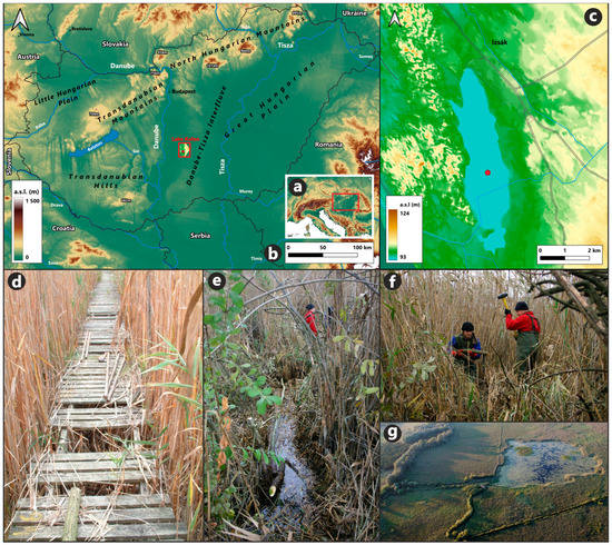
Figure 1.
(a) Location of Hungary in Europe in a red square (1:9,000,000); (b) location of the Izsák—Lake Kolon area (red square) on the geographical map of Hungary (1:2,600,000); (c) coring location (N: 46°46′12.85″ E: 19°20′43.47″) in Lake Kolon (red dot), near the village of Izsák (1:75,000); (d) part of the coring equipment on a wooden bridge on the Lake; (e,f) the process of coring on the lake; and (g) an aerial view [3,4] of the open water surface area of Lake Kolon.
Despite decades of geological research [1,2,3], a comprehensive geochemical description and analysis of the lake is missing. The aim of this research is to fill the gaps left by these previous studies with new magnetic susceptibility, grain size, and loss-on-ignition analyses, and bring in sediment classification, geochemical and PCA analysis to provide a more comprehensive understanding of the developmental history of Lake Kolon. To fully comprehend the impacts of human activity on sediment composition, it is therefore essential to consider the medieval history of the study area, as well as the similar studies in the area conducted by Sümegi et al.: grain size analysis, loss-on-ignition analysis, radiocarbon analysis, and pollen analysis [1]; magnetic susceptibility and malacological analyses [2].
2. Materials and Methods
2.1. Study Area
Lake Kolon is a small (5.5 km in length and 1.5–2.5 km wide, respectively), shallow (60–80 cm) lake located in the Danube–Tisza Interfluve region of Hungary in a depression near the town of Izsák (Figure 1). It is situated on the edge of a glacial alluvial fan in the center of the Pannonian forest-steppe vegetation area. It was formed from a Holocene-era branch of the Danube River that was pushed into the sand ridge between the Danube and Tisza Rivers in a north-south direction [2].
Based on previous and recent studies [1,2,3] and based on the information from the Kiskunság National Park [8,9], the diverse aquatic habitats are surrounded by meadows, marshy forests, and sand dunes. As part of the National Park, the 3058 hectare area has been protected since 1975, with 630 hectares designated as strictly protected. The marshy forests of the Közös-erdő are forest reserve seed areas. Some areas of the lake reach depths of 2–3 m at the old peat mining sites. The area is characterized by a reed swamp, shallow water, and high levels of algae. The lake is home to a diverse range of flora and fauna, including fish species, reptiles, and a variety of birds. Wet grasslands and artificially created open water surfaces provide a habitat for many species. Outside of these, the whole area is covered with reed and is hardly accessible. The lake is known for its rich bird life and is surrounded by planted forests and cultivated fields. It is also experiencing an advanced state of ageing due to sediment accumulation and high levels of organic matter production [3,4]. The whole area is protected and is part of the Little Kiskunság (Cumanian) National Park. Lakebed cleaning and restorations were made between June 2011–February 2013, respectively, which were based on the works of Sümegi et al. [1].
The Walter-Lieth diagram [10] (Figure 2) was created in climatol 3.1.2 [11] in RStudio 2022.07.2 [12] using data provided by the National Meteorological Service [13,14] for the city of Kecskemét (113 m above sea level) between November 2011 and October 2022, respectively (a period of 10 years). Kecskemét has a meteorological monthly data log history dating back to 2011 and is located approximately 26 km from the study site, making it the most suitable location for the analysis. The mean annual temperature is 12.1 °C with an annual precipitation of 514 mm, respectively. The most probable frost months are from October to April, when the absolute monthly minimums are equal to or lower than 0 °C. The precipitation graph shows that August is an arid period, with the highest chance for a draught event, as indicated by the dotted red vertical lines. The period with the highest precipitation is in June, with a range from 60 to 80 mm, respectively. The average minimum temperature was recorded in January (−12 °C), while the average maximum temperature (36 °C) was recorded in August, respectively (Figure 2).
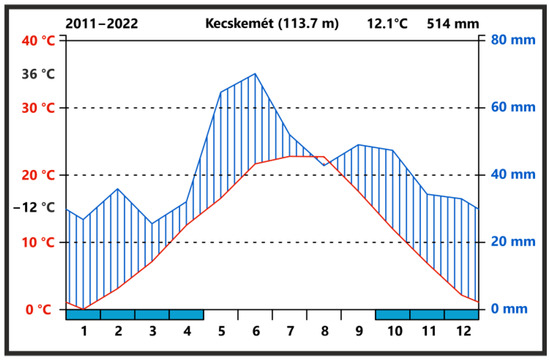
Figure 2.
Walter-Lieth diagram [10] of Kecskemét between 2011–2022. The red-coloured values show the temperature, and the blue-coloured values show the precipitation during the 12 months on average. Probable frost months are marked with blue colour on the bottom scale.
2.2. Sampling and Stratigraphy
Two 440 cm long peat core was collected using a Russian peat corer (5 cm in diameter) with an overlapping method [15,16] in 2007 (Figure 1 and Figure 3): one was previously analysed in [1,2], meanwhile the other has been analysed in this article (N: 46°46′12.85″ E: 19°20′43.47″). The extracted 30 cm long sections were placed in plastic foil, and then in aluminum foil for proper storage in cool, dark conditions (4 °C) until further analysis. The Troels-Smith sediment classification [17] and Munsell colour identification [18] of the samples were performed in the field during the sampling process. During the sampling process, the wind-blown sand presented challenges due to the utilization of a Russian head corer, which is specifically designed for drilling loose and peaty sediments.
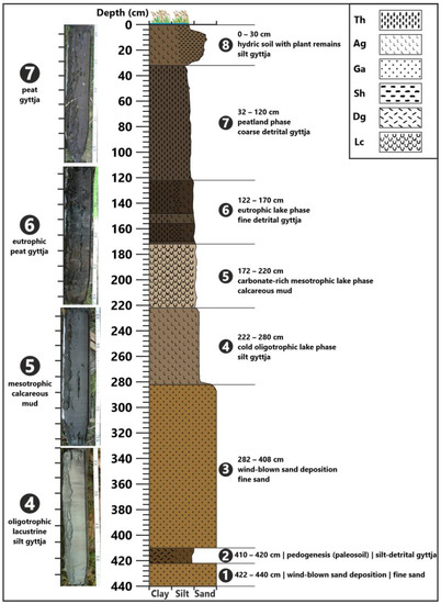
Figure 3.
The lithology of the core based on previous studies [1,2,3] and the results of this article. Eight zones can be differentiated, which are marked by black dots with white numbers, and which are used in the article for consistency. Short descriptions for all zones with boundaries, past environment, sediment type, and Troels-Smith [17] sediment types (Th—reed peat; Ag—silt/aleurite; Ga—fine sand; Sh—humous substance; Dg—mud with plant remains, and Lc—calcareous mud). Lithology colours are Munsell colours [18]. On the left side, core samples are shown which represent the lake and peatland phases, and the scale intervals represent approximately 5 cm each.
2.3. Radiocarbon Dating
Conventional radiocarbon ages were derived from previous studies conducted on the sibling core [1,2]. Age-depth modelling (Bacon) and the estimation of the sedimentation rate (accrate.depth) was conducted using RBacon 2.5.8 [19] in Rstudio 2022.07.2 [12], Build 461, and the IntCal20 calibration curve [20,21]. BP and BC/AD dates used in the text and figures are the calibrated median ages.
2.4. Magnetic Susceptibility, Grain Size, and Loss on Ignition
Bulk samples underwent magnetic susceptibility analysis [22]. Samples were taken at 4 cm intervals (110 samples) and were first crushed in a glass mortar after weighing. The samples were then placed in plastic boxes and air-dried in an oven at 40 °C for 24 h. The magnetic susceptibilities of the samples were then measured at a frequency of 2 kHz using a Bartington MS2 magnetic susceptibility meter with an MS2E high-resolution sensor [23]. Each sample was measured three times, and the average values of magnetic susceptibility were calculated and reported. This non-destructive method enabled the utilization of the same samples for other analyses as well.
The grain size data of the pretreated sediment core samples were obtained at 4 cm (110 samples) intervals for 42 grain-size classes ranging from 0.1 µm to 500 µm, respectively, using laser diffraction with the OMEC Easysizer20 laser particle size analyser [24]. Easysizer20 performs all measuring steps automatically after the initial parameter setup, which provides easy operation and accurate results.
The organic matter, inorganic matter, and carbonate content of the samples were determined using the loss-on-ignition method. The core was cut into 1 cm thick samples, and every second sample was utilized (with a 2 cm sample interval; 220 samples). Initially, the empty ceramic containers were weighed, and then the samples were placed in the crucibles and dried at 105 °C for 24 h in a laboratory furnace. After cooling to room temperature, the samples were powdered. Given their high water content, it was not recommended to powder or crush peat samples before drying. Subsequently, the dried samples in the crucibles were weighed and placed in a furnace again for 1 h at 550 °C to ignite the organic carbon (OM or LOI550). The samples were weighed again after cooling to room temperature. Third, the samples were put into the furnace for 1 h at 900 °C and, after cooling to room temperature, the weight lost was equal to the carbonate content (CC or LOI900). The residuum (IM or LOIres) represents the inorganic matter content [25,26].
2.5. Geochemical Analysis
The water-soluble element contents (Ca, Mg, Na, K, Fe, Mn, Al, P, Zn, and Ti, respectively) of the samples, taken at 2 cm intervals (140 samples), were exactly determined using the five steps sequential extraction geochemical analysis method developed by Dr. Péter Dániel [27,28]. Sequential extraction methods have been widely used to analyse the geochemical composition of materials. These methods involve the use of specific solutions and protocols to extract different forms of elements and compounds from a sample. Common techniques include the use of hydrogen peroxide (H2O2) for removing organic matter, and dithionite-citrate-bicarbonate (DCB) for extracting various forms of Fe, Al, Si, Mn, and Ti. Lakanen–Erviö extraction was also recommended following the DCB treatment. Results from these methods have provided valuable insights into the properties and characteristics of the different materials.
Before the five steps (displayed below), the homogenous sample must be dried to remove any moisture. Prior to the first extraction and between each different extraction step, water extraction (20 ml distilled water for 10 min in repeated twice) was used for cleaning the sample to avoid the dissolution of residual ions mobilized by the former step. These five steps, along the dissolved materials, are as follows:
- Water extraction to obtain water-soluble ions from weathered minerals, carbonates, salts, and precipitates, and ions bound slightly on mineral surfaces;
- Extraction with an NH4-acetate/acetic acid buffer to obtain the ions of carbonates, precipitates, gels and allophans;
- DCB extraction to obtain the ions of Al, Fe, Mn, and Ti-containing oxy-hydroxy-gels;
- Extraction with acid Na2EDTA to obtain the ions of the remaining carbonates, gels, allophanes, and ions bound strongly on mineral surfaces;
- Wet total digestion of the cleaned crystalline fraction with 65% HNO3 and 35% HF to obtain ions of well-crystallized carbonate-, gel-, and allophan-free minerals.
2.6. Statistical Analysis
Statistical analysis was performed using PAST 3 Paleontological Data Analysis software [29]. Principal component analysis was used to identify the main factors that control elemental distribution in the core section. Before analysis, all data were converted to Z-scores calculated as (Xi − Xavg)/Xstd, where Xi is the variable and Xavg and Xstd are the series average and standard deviation, respectively, of the variable Xi [30,31].
3. Results
3.1. Radiocarbon, Magnetic Susceptibility, Grain Size, and Loss-on-Ignition Analysis
Figure 4 and Figure 5 indicate a rapid and monotonous deposition in the bottom part (Zones 1–4), which are all different lake environments. The deposition of calcareous sediment (Lc4) in Zone 5 is slower compared to the previous zones. The first part of the peat accumulation (Zone 6) shows an increased rate (similar to Zones 1–4), where about 50 cm of sediment accumulated in just over a thousand years. From approximately 10,000 BP (120 cm), the accumulation rate increases as the peat bog environment expands, indicating that the time needed for the same sediment to accumulate increases, and organic matter-rich sediment deposits classified as Th4 are formed (Zone 7). The accumulation rate becomes rapid again in the top part of the sequence (Zone 8). In this Zone, bottom lake sediment interruptions and changes are expected due to the anthropogenic presence in the area. To gain a deeper understanding of the data, calibrated modelled dates from radiocarbon analysis were assigned to every 20 cm increment in Figure 5.
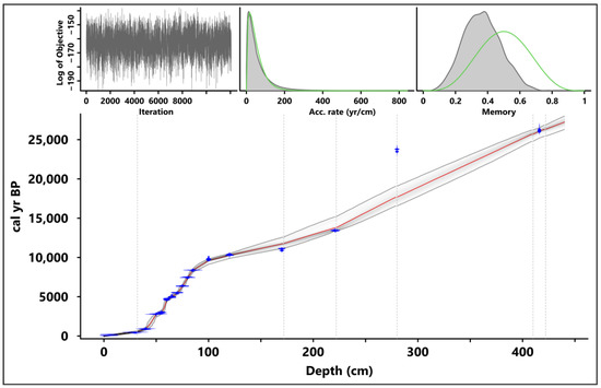
Figure 4.
Radiocarbon model made in RStudio [12] with rbacon [19]. Details of modeling: acc.shape: 1.5; acc.mean: 50; mem.strength: 10; and mem.mean: 0.5; 222 pieces of 2 cm sections.
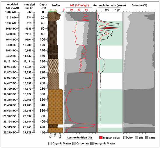
Figure 5.
Combined figure of (from left to right) the modeled calibrated BC/AD and BP median dates from the radiocarbon analysis; lithology profile (Figure 3); magnetic susceptibility (red line) with LOI (%) results (3 shades of grey); accumulation rate from the radiocarbon analysis with median values (red line), with min and max values (black line) and white-green stripes for zone indication; and the summarized grain size (%) results of the clay, silt and sand fractions (shades of gray).
The MS (Figure 5) exhibits low values in Zones 1 and 3, meaning the wind-blown sands in this sequence have low magnetic characteristics. It is increasing towards and in Zone 2, reaching its maximum, and then slowly declines in Zone 3, indicating that it is correlated with the paleosoil deposition. The MS then increases once again towards and in Zone 4, where the second-highest values are displayed for a longer distance. Reaching Zone 5, the MS value suddenly drops, and exhibits fluctuating values between 40–50. It is followed by an increase in Zone 6, with a sudden drop and recovery. In Zone 7, it decreases suddenly again and shows low fluctuating values, with a sudden drop like in Zone 6. In Zone 8, it has a quick increase, followed by a sudden drop, a slower recovery, and a slower drop up until the surface.
Figure 5 presents the results of the grain size analyses, providing a summarized overview, while Figure 6 offers an extended representation, and Figure 7 shows a ternary diagram. The analysis reveals a predominance of bottom sand (Zones 1 and 3) with a minor silt peak (Zone 2). This is followed by silt dominance (Zone 4) and subsequent zones (Zone 5–7) characterized by silt dominance, accompanied with fluctuations in clay content and varying sand grain sizes. In Zone 8, the clay content reached its maximum, and there was a significant increase in sand, although silt remained the dominant category. The detailed examination in Figure 7 uncovers the dominance of silt, silt loam, and sand as the prominent grain size categories. Additionally, noteworthy categories, such as loamy sand, loam, and silty clay loam are also observed.
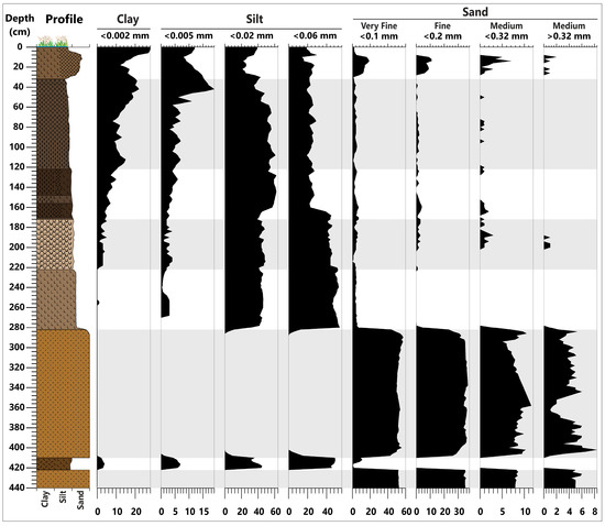
Figure 6.
Results of the grain size analysis with clay (<0.002 mm), silt (0.002–0.06 mm), and sand (>0.06 mm) fractions.
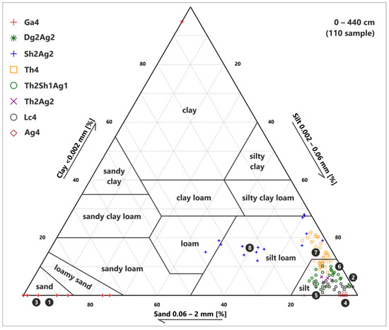
Figure 7.
Ternary diagram of clay, silt, and sand grain sizes with Troels-Smith [17] sediment types based on the grain size analysis and zones (1–8).
In Zones 1 and 3, larger grain sizes are present, specifically very fine sand, which consists of 50–60% 0.06–0.1 mm, 30–35% 0.1–0.2 mm (fine sand), 5–10% 0.2–0.32 mm (medium sand), and 2–4% > 0.32 mm (medium sand) grain size fractions, respectively. There is an absence of sediment in the range of 0–0.06 mm in Zones 1 and 3. The grain size <0.32 mm peaks are around 360 cm, and subsequently declines in a slope-like form. Larger grain sizes (>0.06 mm) were consistently correlated with inorganic matter content throughout the entire sequence. In Zone 2, there was a sudden increase in the proportion of lower grain-sized sediments (silt), with greater than 80% of the samples falling within the range of 0.005 mm to 0.06 mm, respectively, and a complete absence of sediment above 0.1 mm in grain size. In Zone 4, smaller grain sizes became prevalent, and these were found to be correlated with the increased carbonate and organic matter content. From the start of Zone 4, the proportion of sediment within the range of 0.02–0.06 mm (coarse silt) quickly increased to 44–54%, before subsequently decreasing to 14–30% from 164 cm, respectively (Zone 6). The proportion of sediment within the range of 0.005–0.002 mm (fine silt) increased from 35–45%, reaching a peak in Zone 7, before declining to around 20% in Zone 8, respectively.
A slight but consistent increase in the sand, more specifically in the proportion of higher grain sizes (>0.06 mm), was observed from Zone 5 up until the surface, with a peak between 30–10 cm. The proportion of clay (sediment below 0.002 mm) continuously increased from Zone 5 up to the surface, reaching a peak at 0 cm. The proportion of sediment within the range of 0.002–0.005 mm also increased continuously from Zone 4, reaching a peak at around 45 cm, before declining (sand peak near the surface), and then increasing again. The grain size ranges most closely associated with peat accumulation and organic matter was between 0.002–0.02 mm, respectively, although this range also indicates the presence of the lake and bog phases, where there is a consistent water supply and organic accumulation.
The accumulation of organic matter is closely related to peat accumulation and the presence of plant remains (Figure 5). The absence of organic matter content (0%) occurred between 440–422 cm and 408–282 cm (Zones 1 and 3), respectively, indicating no peat or organic matter accumulation. Zone 2 marked the initial evidence of organic matter (between 15–30%), suggesting the onset of a small-scale organic sediment accumulation. In Zones 4 (0.1–0.9%) and 5 (2.1–4.8%), the wetland environment exhibited a low and stagnant organic deposition. Over thousands of years, there has been a slight increase in organic matter content, indicating the development of a more extensive and vegetated environment. At 172 cm, a significant shift occurred, denoting the establishment of a peatland environment. The acceleration of organic matter accumulation was observed, with the deposition of peat containing a low organic matter content in Zone 6 (35.7–49.3%). In Zone 7, the organic matter content experienced a sudden increase, reaching a range of 59–65.4% (120–44 cm), with its maximum at 42 cm (67.2%), respectively, followed by a decrease (40–32 cm, 38.9–66.7%). Towards the surface (Zone 8), there was a substantial decrease in organic matter content (30–0 cm, 5.7–9.7%).
Throughout the core sequence (Figure 5), the presence of carbonate content is primarily linked to changes in inorganic matter and demonstrates an increase during the carbonate-rich lake phase. In the lower part of the core (Zone 1–4, 440–266 cm), the carbonate content fluctuated and ranged between 0.5–7.3%. Beyond 266 cm, the carbonate content exhibited an increase and became less variable, ranging between 10–12% within the range of 264 cm to 222 cm, respectively (Zone 4). Zone 5, characterized with a calcareous lacustrine environment, accumulates a high carbonate content (58–69%). In Zones 6–7, the carbonate content ranged between 11–18%, and gradually decreased with minimal fluctuation. In Zone 8, the carbonate content experiences a subsequent increase until 22 cm (22–25%), after which it gradually declined towards the surface, ranging between 5–12%, respectively.
Inorganic matter content (Figure 5) dominates the bottom 440–222 cm and the top 30–0 cm intervals. In Zones 1 and 3, it has a value interval of 93.1–97.7%, and in Zone 2, it has a value interval of 64.4–83.8%, respectively. In Zone 4, inorganic matter content slowly decreased from 96.5% to 87.7%, respectively. In Zone 5, its value suddenly dropped down and stayed around 26.3–37.7%. In Zone 6, inorganic matter content increased to 31.4–46.9%. In Zone 7, its value decreased down to 17.3–27.3%, and near the surface, it began to quickly increase to 66–91%, which was deemed to be possibly due to the recent erosions.
3.2. Sediment Classification
Troels-Smith classifications [17] were performed at the study site during sample collection, and since the samples were removed from a wet environment, there is a possibility of an imprecise classification of the smaller grain sizes. Comparison of the Troels-Smith classifications [17] with grain size measurements (Figure 5, Figure 6 and Figure 7) revealed a much lower clay content and dominant silt grain size between the depths of 0–280 cm (Zones 4–8) and 410–422 cm (Zone 2), respectively. Therefore, the Troels-Smith classifications [17] in the figures and text, specifically the As (clay) content between these depths, should be Ag (silt/aleurite) instead based on grain size analysis. To provide a more precise description and classification, Sh2As2, Th2Sh1As1, Th2As2, Ag2As2, and Dg2As2 should be corrected to Sh2Ag2, Th2Sh1Ag1, Th2Ag2, Ag4, and Dg2Ag2, respectively. These corrected versions were used instead of the on-site determined classifications [17] in all the presented figures in this study and in the text when discussing the different phases.
The first 280 cm of the sequence includes a hydric topsoil layer (Zone 8) composed of humous substances and silt-sized mineral particles (Sh2Ag2). In Zones 7 and 6, there was a peat layer observed followed by a mixture of peaty humous matter and silt-sized mineral particles (Th4, and a mix of Th, Sh, and Ag). A carbonate-rich layer was found in Zone 5 (Lc4), followed by soil comprising silt-sized mineral particles in Zone 4 (Ag4). The second part of the sequence began at 280 cm, and extends down to the bottom of the core, up to 440 cm (Zones 1–3). This lower section is mainly composed of very fine sand (Ga4), with a 12 cm thick zone of plant remains and silt-sized mineral particles (Dg2Ag2, Zone 2) [17].
The Polish bottom lake classification system (Figure 8) [32,33], which is based on loss-on-ignition analysis data, was used to differentiate between the phases and provide a clearer understanding of the evolution and development of the core sequence. With this system, it is thereby possible to interpret the loss-on-ignition data to describe the sediment types, especially if paired with the Troels-Smith classification [17].
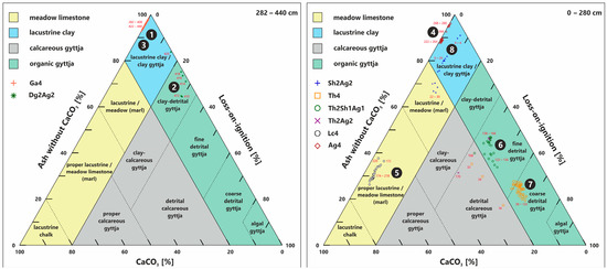
Figure 8.
Results of loss-on-ignition analysis on a ternary plot (organic matter %, inorganic matter %, and carbonate content %). Symbols represent the Troels-Smith classification [17], and the background represents the bottom lake deposit classification system [32,33]. Zones 4–8 are also marked, along with the sample depth values with red-coloured text near the symbols.
The data interpretation revealed that the sequence starts with a very fine-fine sand sediment (Zones 1 and 3), followed by a silt-detrital gyttja phase (Zone 2), a silt gyttja phase (Zone 4), a proper lacustrine limestone phase (Zone 5) with a transition from fine detrital gyttja to coarse detrital gyttja (Zones 6–7), which eventually develops into silt gyttja near the surface (Zone 8). In this context, the terms “fine and coarse detrital gyttja” refer to the partially or completely decomposed reed and sedge peat mixed with inorganic sediment. Similarly, the term “proper lacustrine limestone” denotes calcareous mud. The substitution of clay with silt has been attributed to its limited volume based on grain size analysis. Silt gyttja may occur in the uppermost layers of deposits as a parent material for soils and at the bottom of an oligotrophic lake phase.
3.3. Geochemical Analysis
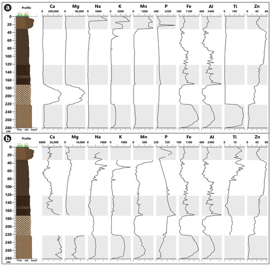
Certain elements exhibited significant peak values in specific depths and intervals, which overshadow the minimum and average values on the diagrams, indicative of a localized accumulation or concentration of these elements. Consequently, it is crucial to not only examine the prominent results depicted in Figure 9, but to also investigate the lower yet significant and important values and changes (Figure 10). For this purpose, the following depth intervals, indicating the maximum ppm values for different elements, were extracted in cm as follows: Na 0–10 cm, K 0–30 cm, Mn 0–30 cm, P 22 cm, and Ti 222–280 cm, respectively. In the case of Fe, Al, and Zn, this process was not required as the ppm value changes were visible and were not overshadowed by the much greater peaks. The geochemical result discussions below are based on Figure 9 and Figure 10.
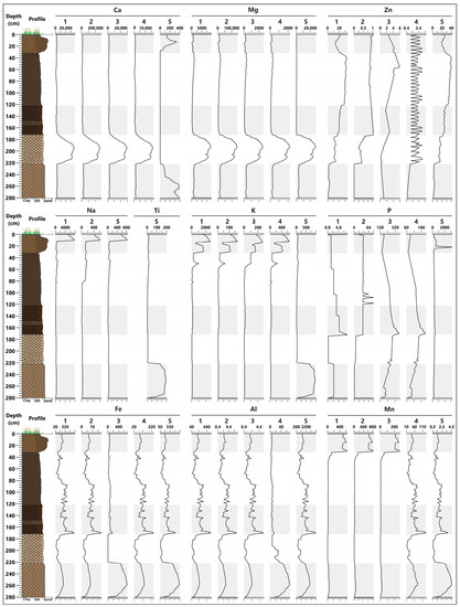
Figure 9.
Results of the five-step sequential extraction method [27,28] for every element. All values are in ppm. Steps: 1 = water extraction; 2 = NH4-acetate/acetic acid buffer (pH = 5) extraction; 3 = dithionite-citrate-bicarbonate extraction; 4 = Lakanen–Erviö extraction; and 5 = wet total digestion of the crystalline fraction.
The presence of inorganic accumulation was deemed to be accountable for the occurrence of Ca (33,000–39,200 ppm) and Mg (4300–12,500 ppm) in Zone 8, where their changes were interconnected and exhibited a correlation until the initiation of Zone 6. The highest concentrations of Ca and Mg were found in Zone 5, with Ca ranging from 83,409–343,814 ppm, and Mg ranging from 12,500–55,200 ppm, respectively. The origin of Ca possibly comes from the Chara vegetation overgrowing the lake bottom and influencing the sedimentation biologically, which accumulates high amounts of CaCO3 as a result [1,3]. Ca demonstrates a consistent decline from 34,700 ppm to 13,300 ppm within the depth interval of 170–142 cm, respectively. However, it gradually increases between 140–116 cm (13,900–24,100 ppm) and 58–0 cm (7600–22,400 ppm), followed by a decrease between 114–60 cm (6538–22,892 ppm), respectively. Mg underwent a slow and monotonous decline after Zone 5, reaching 560 ppm at 146 cm, then gradually increased to 4400 ppm at 42 cm. In Zone 8, Mg experienced an overall decrease and ranged between 700–3000 ppm.
The K content in Zone 4 (539–1067 ppm) was most likely derived from mineral sources, displaying a sudden decrease in Zone 5 (66–134 ppm). Within Zone 6, it fluctuated around 200 ppm. A lower-value phase was observed in the first half of Zone 7, followed by an increase and three peaks: the first at 82 cm (359 ppm), the second between 54–46 cm (654–1492 ppm), and the third between 30–18 cm (1765–2503 ppm), respectively. It reached its maximum peak in Zone 8 (12–0 cm, 2464–3808 ppm).
Different analysis steps revealed distinct diagram shapes and trend results for P content, except for steps 3 and 4. The P content increased from Zone 4 until the beginning of Zone 6 (280–170 cm, 341–1017 ppm), followed by a decrease with smaller spikes (168–94 cm, 689–980 ppm) and a slope-like diagram shape (92–28 cm, 450–692 ppm) until Zone 8. In Zone 8, a peak was observed (26–24 cm and 20–8 cm, 550–869 ppm), with the highest value of 3460 ppm at 22 cm. Subsequently, the P content gradually decreased to 468 ppm at 0 cm. Overall, changes in P content were not associated with organic matter content.
The contents of Mn, Fe, and Al demonstrate correlation and change in unison, exhibiting similar diagram shapes between Zones 4 and 7, with the exception of Mn, which diverged from 44 cm. In Zone 4, all three elements initially increased (280–258 cm; Mn 38–224 ppm, Fe 275–2066 ppm, and Al 790–3288 ppm, respectively), followed by a subsequent decrease (256–222 cm; Mn 86–214 ppm, Fe 1287–2043 ppm, and Al 2048–3252 ppm, respectively). Subsequently, they experienced a significant drop to their lowest values in Zone 5 (Mn 18–86 ppm, Fe 117–416 ppm, and Al 462–1484 ppm, respectively). Throughout Zones 6 and 7, they exhibited highly fluctuating diagram shapes and values (Mn 70–114 ppm, Fe 472–1050 ppm, and Al 1344–3086 ppm, respectively), with a peak observed at 170–168 cm (Mn 164–176 ppm, Fe 1456–1649 ppm, and Al 4150–4700 ppm, respectively). Another shared interval of low values was present in the second half of Zone 7 (80–44 cm; Mn 40–103 ppm, Fe 156–611 ppm, and Al 444–1742 ppm, respectively). Following this, Mn initiated an increase (42–32 cm, 172–354 ppm) and reached its maximum in the uppermost 30–0 cm (1332–1741 ppm). Fe and Al also exhibited an increase, albeit with a smaller plateau diagram shape towards the surface (42–0 cm; Fe 254–736 ppm, and Al 693–2006 ppm).
The Ti content, measured in steps 1, 2, 3, and 4, was below the measurement limit. The highest Ti content, measured in step 5, was observed in Zone 4 (11–192 ppm), which experienced a sudden decrease to its minimum values in Zone 5 (5–8 ppm). This value continued to decrease until the middle of Zone 7 (144 cm, 1 ppm), after which it demonstrated an upward trend with values of 1–4 ppm. Starting from 80 cm, the Ti content began to increase and reached 7–19 ppm in Zone 8.
Zn consistently exhibited very low values (3–81 ppm) throughout the entire sequence, and it also presented varying diagram shapes and trend results. The lowest values of Zn were observed in Zone 4 (3–8 ppm), gradually increasing after each zone (Zone 5: 18–35 ppm, and Zone 6: 42–57 ppm, respectively). Zn reached its maximum at 56 cm (81 ppm) in Zone 7 (65–81 ppm). In Zone 8 (37–58 ppm), there was a decrease in value observed, followed by an increase towards the surface.
3.4. Statistical Analysis
Principal component analysis (PCA) was performed on the whole dataset (LOI, MS, GS, and summarized geochemical analyses) to reduce its dimensionality and identify the patterns of variation. The largest proportion of the variance in the data was explained by the first four principal components, making them the most informative for investigation and visualization (Figure 11, Table 1).
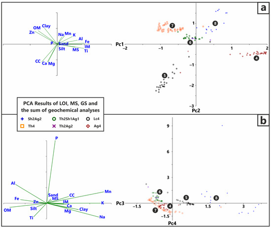
Figure 11.
Results of PC 1 and PC 2 (a), and PC 3 and PC 4 (b) analyses with scatter plots (X and Y axis numbers are eigenvalues) and separate biplots. Symbols indicate Troels-Smith [17] classifications, and white numbers in black circles indicate Zones from 4 to 8.

Table 1.
Eigenvalue, % variance, and loadings for PC 1–PC 4. Different colours indicate negative (red), positive (black), and the first (and second for K, IM, and Clay) greatest loadings (bold, green).
PC1 explains the largest proportion of the variance in the dataset (34.04%), and is dominated by elements of inorganic sedimentological origin, such as K, Fe, Al, Ti, IM, and MS. These elements were found to be associated with Zones 4 and 8, suggesting a contribution from weathering, erosion, and dust processes. Na and Mn also have positive loadings, but to a lesser extent, and they align more towards Zone 8.
PC2 explains 29.24% of the variance, and primarily represents the elements of organic origin. Elements such as Na, K, Zn, Clay, and OM contribute positively to PC2, and are associated with the eutrophic lake and peatland phases in Zones 6 and 7. Other elements like Fe, Al, Mn, and P also contributed, although to a lesser degree due to the continuous accumulation of IM throughout the sequence.
Sand has positive loadings for both PCs in small amounts, but sides with PC 2 were more due to the top 30 cm of the sequence (Zone 8), which accumulated the most sand between Zones 4 and 8. Ca and CC elements show negative loadings towards both PC 1 and PC 2. PC3 explains 19.51% of the variance and is primarily influenced by Zone 5, which exhibited the most positive loadings for elements such as Ca, Mg, and CC. Additionally, Na, K, Mn, IM, and clay also significantly contributed to PC3 and are indicative of Zone 8.
PC4 explains 7.74% of the variance, and exhibited negative loadings for Zones 4, 6, and 7, respectively. The dominance of the P peak in Zone 8 contributed entirely to PC4, indicating a strong association between P and this zone. Al, Mn, and CC also had significant positive loadings in PC4, further emphasizing their contribution to the geochemical variations observed.
In summary, these PCA results indicate that the different phases and environments in the dataset exhibited mixed sedimentological origins and are tied to multiple processes. However, there were notable correlations observed between certain elements, as follows:
(1) Elements of organic origin (Na, K, Zn), clay, and organic matter;
(2) Elements of inorganic origin (Fe, Al, Ti, Na, K, P), MS, sand, and inorganic matter;
(3) Elements of carbonate origin (Ca, Mg) and carbonate content.
4. Discussion
4.1. Paleoenvironment Changes during the Pleistocene
This area is not originated from oxbow lakes since it is separated from the floodplain and the surface floods. Thus, the accumulated sediment did not arise from the Danube floods. The sequence began with a large amount of wind-blown, very fine-fine sand (Zones 1 and 3). Due to the location, this was deemed to be a typical sediment present in the area, forming sand dunes, and playing a fundamental role in soil development. This sandy and loessy sediment possibly originates from the Alps (fluvial, by the Danube) and from the Transdanubian Mountains (aeolian processes) [1,2,3]. The deposition of this sand occurred between 27,000 BP and 17,700 BP, respectively, corresponding to the period of the Last Glacial Maximum and its subsequent stages. As the climate gradually warmed and the ice sheets retreated, the availability of sand sources and prevailing wind patterns influenced the distribution and accumulation of sand in the region. Over time, aeolian sand deposition gradually declined as vegetation cover increased and stabilized the surface. The establishment of vegetation, including grasses and shrubs, acted as a natural barrier, reducing the erosive power of the winds as a result, and aiding in soil formation.
A small detrital gyttja (Zone 2) was present between two sand layers around 26,000 BP, which can be described with this process [34]: when clay/silt gyttja runs off or crawls down the slope, it typically accumulates in the lowest parts of the lake basin, forming thick layers of deposits. Although other possibilities, such as allochthon sediment deposition or a short pedogenesis [1] cannot be ruled out. The formation and development of the lake and wetland deposits are greatly influenced by catchment conditions and the local climate, which can result in various sediments. These environments and sediments have been, in general, widely researched, especially in cases where they are near an archaeological or historical site [24,35,36,37,38,39]. The boundaries of the lake and bog phases can be distinguished, and the development of the lake can be outlined by examining the results together with previous analyses [1,2]. Lacustrine clay and clay gyttja are typically found in the lower parts of the deposit and are relatively rare [40]. However, clay gyttja and clay-detrital gyttja can also be found in the upper layers of deposits (such as between 40–0 cm), where they serve as the parent material of soils [41]. It is noteworthy that multiple samples in this sequence were classified as lacustrine clay (clay gyttja), both at the top and at the bottom of the sequence (Figure 8.). However, due to the minimal amount of clay, which was only present from the oligotrophic phase (Zone 4) and increases towards the surface, silt gyttja and lacustrine silt are being discussed based on the grain size results.
The bottom sand (Ga4) was overlain by lacustrine silt gyttja, which became more calcareous (increasing twice) in Zone 4 (Ag4). Meanwhile, inorganic matter content decreased in favor of the carbonate content and a negligible amount of organic matter. This marks the start of the oligotrophic lake environment at around 17,700 BP years, which is still mainly influenced by allochthonous geological processes (including weathering and aeolian deposition), and the transition from fine sand to silt gyttja. This finding is consistent with [34], who argue that clay gyttja (silt gyttja in this case) is genetically connected to the early stages of lake development when plankton production is low, and therefore these organisms contribute less to the accumulated sediments. Since there is a constant and expected aeolian dust deposition [1] from the nearby sand dunes, the presence of the weathered inorganic mineral sediments and the associated element accumulations were also expected in the whole sequence. This increase in silt fraction was tied to the oligotrophic lake formation. Geochemically, this is the first zone that was investigated. Ca and Mg contents follow the increasing carbonate content. Na, K, Ti, Fe, Al, and Mn concentrations were also high in this part but were still somewhat influenced by allochthonous geological processes. Meanwhile, the P content slowly increased, and the Zn content stayed relatively low.
A change in the environment and the climate could have caused intense weathering and pedogenesis, which resulted in a change that caused the lake to be mainly influenced by biological (autochthonous) processes [1,3]. A Chara-lake formed, which explains the origin of the calcareous mud (Lc4, Zone 5), which overlaid the slightly calcareous lacustrine silt gyttja (Ag4) approximately 13,800 years ago. The development of this calcareous mesotrophic Chara-lake occurred between the middle of the Older Dryas and the end of the Younger Dryas, which is a well-defined synchronous cool period. Organic matter content also increased, reaching around 10%. Ca and Mg contents dominated the calcareous phase; K, Fe, Al, Mn and Ti values decreased extensively, which were of mineral origin; Na slightly decreased and exhibited a dome-like diagram shape; P content increased monotonously; and Zn increased with three small peaks in a zig-zag diagram shape. Calcareous gyttjas, in the form of bog lime (lacustrine chalk), were encountered less frequently, and they are the parent material for quaternary rendzina soils [42]. The most famous and researched lake in Hungary with similar sediment accumulation is in Csólyospálos, where meadow limestone (“darázskő”) forms [35,36]. Csólyospálos is also located in the Danube–Tisza Interfluve, only 55 km away from Lake Kolon.
4.2. Paleoenvironment Changes during the Holocene
The calcareous lacustrine phase was replaced with the continuously increasing vegetation by a mesotrophic lake with a rudimentary bog environment from 172 cm (Zone 6) approximately 11,700 years ago, around the Greenlandian boundary (11,650 BP). This Pleistocene-Holocene boundary indicates rising temperatures and a change in the climatic conditions not only in the Danube–Tisza Interfluve, but also all over the Carpathian Basin. As a result of this, the cold-water oligotrophic lake gradually transformed into a temperate eutrophic lake [1]. From this stage, the main processes influencing the sediment deposition are still of a biological origin (autochthonous), but the source changed from Chara to reed and sedge peat. A relatively fast (around 1500 years) development to an organic-rich state happened: first changing to detrital calcareous gyttja (170–168 cm), then fine detrital gyttja (166–138 cm), and then slowly increasing its organic matter content (136–122 cm). This detrital gyttja has a lower percent of carbonate and a higher percent of inorganic matter (mix of Th-As and some Sh) compared to the previous phase. From the start of this zone (Zone 6), Ca, Mg, Na, Mg, P, Fe, Al, and Ti contents were all found to have decreased, while Zn content increased with K content. Around 10,800 years ago (144 cm), Fe, Al, and Mn contents exhibited a high peak and have since continued with fluctuating values, while Mg, Na, and Ti contents exhibited a low point and have continued with an increasing trend. Overall, from the mesotrophic lake phase, where the organic matter and inorganic matter ratios are the most equal (organic matter 35–49%, inorganic matter 31–46%, and carbonate 11–33%, respectively), a high amount of Fe, Al, Mn, P, Ca, and Zn concentrations were determined from the sediment.
The growth of the peatland environment occurred along with the appearance of the clean Th4 sediment and a high increase in organic matter content (>59%) from 122 cm, approximately 10,300 years ago. This extended peatland phase lasted for nearly 9600 years (Zone 7), until the organic matter accumulation started to decline. The accumulation rate slows down from the start of this phase. From about 7400 years ago (80–82 cm), geochemical changes of anthropogenic origin [1] can be perceived, and the effect of different human cultures must be considered when interpreting the results. Between 82–32 cm, all of the elements assessed exhibited either an increasing or a decreasing pattern: Mg, Na, K, Mn, Ti and Zn all increased, Ca decreased and increased, while Fe, Al, and P all decreased heavily. The accumulation rate slowed down drastically, reaching the slowest sedimentation in this zone. Na and K are typically associated with organic matter and living plants, and their values tend to decrease with depth, exhibiting higher values near the surface. This “fresh” organic Na and K content, along with the inorganic Na and K contents, can be observed in the top cca. 50 cm (in the past 4000 years). Zn content has also been associated with the vegetation, increasing with the organic matter content towards the surface. In soils with higher pH values (>7), like in this wetland, Zn is adsorbed more easily [43].
The peat slowly backtracked to detrital calcareous gyttja (Zone 8) and kept its carbonate content (36–32 cm), while decreasing their organic matter and increasing their inorganic matter content. This anthropogenic effect was observed in the increase of the Ca, P, and Mn contents near the surface. The first decrease in organic matter at 36 cm was dated as 942–579 BP, with a median of 732 BP (1008–1371 AD, 1218 AD median). This decrease was associated with the inhabitation and settling of the nearby area by the stablemen of the Tihany Abbey [44] during the Kingdom of Hungary (1000–1301 AD) to raise and keep the horses of the Tihany Abbey. After this, the immediate area of the lake was constantly inhabited and influenced by the Hungarian people living there. The sediment changes to calcareous mud with an inorganic matter dominance (30–22 cm), followed by a silt gyttja phase (20–0 cm) with an increasing inorganic matter content. The amount of clay reached its maximum near the surface, meaning the silt gyttja classification came the closest to the clay gyttja in this interval, which correlated with its function to act as a parent material to soils [41].
Today, the remnants of the aeolian sand deposits can still be observed in the immediate vicinity of the lake, providing valuable insights into the past climatic conditions and the geomorphic processes that shaped the region. Although there was no agriculture across much of the area, continuous habitat management and development are still necessary to maintain these diverse habitats, along with the continuous eradication of invasive alien species which serves to preserve the vegetation of the sand hills [8,9]. Proper grassland management preserves the valuable plant and insect life of the meadows. Adequate habitat protection is an essential condition for regular monitoring activities. The entire protected area serves nature conservation purposes, but at the same time, people living in the surrounding settlements are rediscovering Kolon Lake and getting to know its wildlife [8,9].
5. Conclusions
The key focus of paleoenvironmental research is the comprehension of lacustrine sedimentation processes in response to the past natural and human-induced environmental, hydrogeological, and climatic changes. Such changes are particularly likely to affect lacustrine systems, like the one presented here, given their restricted size and shallow water levels, as well as the nature of their major water and sediment sources. Around 27,000 years of changes and development can be seen through the eyes of the different sand and lake sediments. About 10,000 years of sand deposition gives the bottom of the sequence. The gradual increase in vegetation cover stabilized the surface and reduced aeolian sand deposition, which gave birth to oligotrophic lake sediment accumulation from around 17,700 BP, followed by the mesotrophic Chara-lake, an environment containing calcareous mud/chalk sediments from around 13,800 BP. Organic-rich vegetation and peat (reed, sedge) accumulation starts at the border of the Pleistocene and Holocene Epochs at around 11,700 BP, at the beginning of the Greenlandian age, and at the start of the rising temperatures and the changing climate. The organic matter content was found to be related to peat accumulation and plant remains, with a significant change observed in the emergence of a peatland environment. From around 10,300 BP, the percentage of peat increased significantly. Notable changes occurred from around 9000–8000 BP due to the different emerging cultures in the Carpathian basin, and from around 942–579 BP due to the Hungarian settlements and activity nearby, respectively. Elements exhibited varying concentrations, reflecting the interplay of environmental factors, vegetation, and human activities. A strong correlation can be observed among the different phases and environments, despite their mixed sedimentological origins and the involvement of multiple processes. Specifically, correlations were noted between (1) clay, organic matter, and elements of organic origin (Na, K, and Zn); (2) MS, sand, inorganic matter, and elements of inorganic origin (Fe, Al, Ti, Na, K, and P); and (3) carbonate content and elements of carbonate origin (Ca and Mg).
Understanding these paleoenvironmental changes provides insights into the dynamic nature of the landscape and its responses to climatic and environmental shifts over time. Further geochemical studies (XRF and XRD) could provide more insights into the connection between the vegetation, and more importantly the mineral composition of Lake Kolon. Furthermore, conducting more radiocarbon analysis can increase the precision of the age-depth models and the accumulation rates. In conclusion, this study has furnished the essential geochemical and sedimentological insights which significantly contribute to the comprehensive understanding of sediment accumulation and environmental changes in Lake Kolon.
Author Contributions
Conceptualization, T.Z.V. and P.S.; Funding acquisition, T.Z.V. and P.S.; Investigation, T.Z.V.; Methodology, T.Z.V.; Supervision, S.G. and P.S.; Visualization, T.Z.V.; Writing—original draft, T.Z.V.; Writing—review and editing, T.Z.V. All authors have read and agreed to the published version of the manuscript.
Funding
This research was funded by the National Research, Development, and Innovation Office (NKFIH), grant number ÚNKP-22-3-SZTE-466.
Data Availability Statement
Data is available upon request from the corresponding author.
Acknowledgments
This research has been carried out within the framework of University of Szeged, Interdisciplinary Excellence Centre, Institute of Geography and Earth Sciences, Long Environmental Changes Research Team. In addition, the authors are also grateful to the three reviewers who helped to improve the quality of this publication. Partial support was provided by the Ministry of Human Capacities, Hungary from grants NKFIH Grant 129265, Grant 20391-3/2018/FEKUSTRAT, and GINOP-2.3.2-15-2016-00009 ‘ICER’.
Conflicts of Interest
The authors declare no conflict of interest. The funders had no role in the design of the study; in the collection, analyses, or interpretation of data; in the writing of the manuscript; or in the decision to publish the results.
References
- Sümegi, P.; Molnár, M.; Jakab, G.; Persaits, G.; Majkut, P.; Páll, D.; Gulyás, S.; Jull, A.J.T.; Törőcsik, T. Radiocarbon-Dated Paleoenvironmental Changes on a Lake and Peat Sediment Sequence from the Central Great Hungarian Plain (Central Europe) During the Last 25,000 Years. Radiocarbon 2011, 53, 85–97. [Google Scholar] [CrossRef]
- Sümegi, P.; Molnár, D.; Náfrádi, K.; Makó, L.; Cseh, P.; Törőcsik, T.; Molnár, M.; Zhou, L. Vegetation and land snail-based reconstruction of the palaeocological changes in the forest steppe eco-region of the Carpathian Basin during last glacial warming. Glob. Ecol. Conserv. 2022, 33, e01976. [Google Scholar] [CrossRef]
- Iványosi-Szabó, A. Az Izsáki Kolon-tó üledék- és környezetföldtani vizsgálata. Ph.D. Thesis, University of Szeged, Szeged, Hungary, 1984. (In Hungarian). [Google Scholar]
- European Environment Agency. Average Annual Precipitation in the EEA Area. Available online: https://www.eea.europa.eu/data-and-maps/figures/average-annual-precipitation (accessed on 7 June 2023).
- Birks, H.J.B.; Birks, H.H. Quaternary Palaeoecology; Edward Arnold: London, UK, 1980; pp. 1–280. [Google Scholar]
- Gaillard, M.-J.; Birks, H.H. Paleolimnological applications. In Encyclopedia of Quatermary Science; Elias, S.A., Ed.; Elsevier: New York, NY, USA, 2007; Volume 3, pp. 2337–2355. [Google Scholar]
- Berglund, B.E. Handbook of Holocene Palaeoecology and Palaeohydrology; John Wiley & Sons Ltd.: Chichester, UK, 1986. [Google Scholar]
- Kolon-tó [Lake Kolon]. Available online: www.kolon-to.com (accessed on 15 May 2023).
- Kiskunsági Nemzeti Park [Kiskunság National Park]. Available online: https://www.knp.hu/hu/kolon-to (accessed on 15 May 2023).
- Walter, H.; Lieth, H. Klimadiagramm Weltatlas; G. Fischer: Jena, Germany, 1960. [Google Scholar]
- The Climatol R Package. Available online: http://www.climatol.eu (accessed on 15 May 2023).
- RStudio Desktop—Posit. Available online: https://posit.co/download/rstudio-desktop/ (accessed on 15 May 2023).
- Országos Meteorológiai Szolgálat. Available online: https://www.met.hu (accessed on 15 May 2023).
- Országos Meteorológiai Szolgálat—Meteorológiai Adattár. Available online: https://odp.met.hu (accessed on 15 May 2023).
- Aaby, B.; Digerfeldt, G. Sampling techniques for lakes and mires. In Handbook of Holocene Palaeoecology and Palaeohydrology; Berglund, B.E., Ed.; John Wiley & Sons: Chichester, UK, 1986; pp. 181–194. [Google Scholar]
- Vleeschouwer, F.; Chambers, F.; Swindles, G. Coring and sub-sampling of peatlands for palaeoenvironmental research. Mires Peat 2010, 7, 10. [Google Scholar]
- Troels-Smith, J. Characterization of unconsolidated sediments. Dan. Geol. Unders. 1955, 4, 10. (In Danish) [Google Scholar]
- Munsell Color. Munsell Soil Color Charts; Munsell Color Company. Inc.: Baltimore, MD, USA, 1954. [Google Scholar]
- rbacon: Age-Depth Modelling Using Bayesian Statistics. Available online: https://cran.r-project.org/web/packages/rbacon/index.html (accessed on 15 May 2023).
- Blaauw, M.; Christen, J.A. Flexible paleoclimate age-depth models using an autoregressive gamma process. Bayesian Anal. 2011, 6, 457–474. [Google Scholar] [CrossRef]
- Reimer, P.; Austin, W.; Bard, E.; Bayliss, A.; Blackwell, P.; Ramsey, C.B.; Butzin, M.; Cheng, H.; Edwards, R.L.; Friedrich, M.; et al. The IntCal20 Northern Hemisphere Radiocarbon Age Calibration Curve (0–55 cal kBP). Radiocarbon 2020, 62, 725–757. [Google Scholar] [CrossRef]
- Oldfield, F.; Thompson, R.; Barber, K.E. Changing atmospheric fallout of magnetic particles recorded in recent ombrotrophic peat sections. Science 1978, 199, 679–680. [Google Scholar] [CrossRef]
- Dearing, J. Environmental Magnetic Susceptibility: Using the Bartington MS2 System; Chi Publishing: Keniloworth, UK, 1994. [Google Scholar]
- Sümegi, P.; Náfrádi, K.; Molnár, D.; Sávai, S. Results of paleoecological studies in the loess region of Szeged-Öthalom (SE Hungary). Quat. Int. 2015, 372, 66–78. [Google Scholar] [CrossRef]
- Dean, W.E. Determination of carbonate and organic matter in calcareous sediments and sedimentary rocks by loss on ignition; comparison with other methods. J. Sediment. Petrol. 1974, 44, 242–248. [Google Scholar]
- Heiri, O.; Lotter, A.F.; Lemcke, G. Loss on ignition as a method for estimating organic and carbonate content in sediments: Reproducibility and comparability of results. J. Paleolim. 2001, 25, 101–110. [Google Scholar] [CrossRef]
- Dániel, P. Results of the geochemical analysis of the samples from Bátoliget II profile. In The Geohistory of Bátorliget Marshland; Sümegi, P., Gulyás, S., Eds.; Archaeolingua Press: Budapest, Hungary, 2004; pp. 95–128. [Google Scholar]
- Dániel, P.; Kovács, B.; Gyori, Z.; Sümegi, P. A Combined Sequential Extraction Method for Analysis of Ions Bounded to Mineral Component. In Proceedings of the 4th Soil and Sediment Contaminant Analysis Workshop. Lausanne, Switzerland, 23–25 September 1996; p. 396. [Google Scholar]
- Hammer, O.; Harper, D.A.T.; Ryan, P.D. PAST: Paleontological statistics software package for education and data analysis. Palaeontol. Electron. 2001, 4, 9–18. [Google Scholar]
- Eriksson, L.; Johansson, E.; Kettaneh-Wold, N.; Wold, S. Introduction to Multi- and Megavariate Data Analysis Using Projection Methods (PCA & PLS); Umetrics AB: Umea, Sweden, 1999. [Google Scholar]
- Davis, J.C. Statistics and Data Analysis in Geology; John Wiley & Sons Inc.: New York, NY, USA, 1986; p. 656. [Google Scholar]
- Kabała, C.; Charzyński, P.; Chodorowski, J.; Drewnik, M.; Glina, B.; Greinert, A.; Hulisz, P.; Jankowski, M.; Jonczak, J.; Łabaz, B.; et al. Polish Soil Classification, 6th edition—Principles, classification scheme and correlations. Soil Sci. Annu. 2019, 70, 71–97. [Google Scholar] [CrossRef]
- Łachacz, A.; Nitkiewicz, S. Classification of soils developed from bottom lake deposits in north-eastern Poland. Soil Sci. Annu. 2021, 72, 1–14. [Google Scholar] [CrossRef]
- Uggla, H. Charakterystyka gytii i gleb gytiowych Pojezierza Mazurskiego w świetle dotychczasowych badań Katedry Gleboznawstwa WSR w Olsztynie [In Polish with English Summary: Characteristics of gyttja and gyttja soils of Mazurian Lakeland in light of hitherto investigations of the Chair of Pedology, College of Agriculture in Olsztyn]. Zesz. Probl. Postępów Nauk Rol. 1971, 107, 14–25. [Google Scholar]
- Molnár, M.; Futo, I.; Svingor, É.; Sümegi, P. Review of Holocene lacustrine carbonate formation in the light of new radiocarbon data from a site of Csólyospálos, Central Hungary. ATOMKI Annu. Rep. 2006, 21, 52. [Google Scholar]
- Jenei, M.; Gulyás, S.; Sümegi, P.; Molnár, M. Holocene Lacustrine Carbonate Formation; Old Ideas in the Light of New Radiocarbon Data from a Single Site in Central Hungary. Radiocarbon 2007, 49, 1017–1021. [Google Scholar] [CrossRef]
- Sümegi, P.; Molnár, D.; Sávai, S.; Náfrádi, K.; Novák, Z.; Szelepcsényi, Z.; Törőcsik, T. First radiocarbon dated paleoecological data from the freshwater carbonates of the Danube-Tisza Interfluve. Open Geosci. 2015, 7, 40–52. [Google Scholar] [CrossRef]
- Knipl, I.; Sümegi, P. A Duna-Tisza közi Hátság és a Kalocsai Sárköz Hajós és Császártöltés községek közötti határterületének geoarcheológiai elemzése. In Geoszférák 2014; Unger, J., Pál-Molnár, E., Eds.; Földtani és Őslénytani Tanszék: Szeged, Hungary, 2015; pp. 85–107. [Google Scholar]
- Achterberg, I.; Eckstein, J.; Birkholz, B.; Bauerochse, A.; Leuschner, H. Dendrochronologically dated pine stumps document phase-wise bog expansion at a northwest German site between ca. 6700 and ca. 3400 BC. Clim. Past 2018, 14, 85–100. [Google Scholar] [CrossRef]
- Markowski, S. Struktura i właściwości podtorfowych osadów jeziornych rozprzestrzenionych na Pomorzu Zachodnim jako podstawa ich rozpoznawania i klasyfikacji. Kreda Jeziorna Gytie 1980, 2, 45–55. [Google Scholar]
- Uggla, H. Gleby gytiowe Pojezierza Mazurskiego. I. Ogólna charakterystyka gleb gytiowo-bagiennych i gytiowo-murszowych. Zesz. Nauk. WSR W Olsztynie 1969, 25, 563–582, (In Polish with German Summary). [Google Scholar]
- Uggla, H. „Rędziny” Pojezierza Mazurskiego. Rocz. Glebozn. 1976, 27, 113–125, (In Polish with English Summary). [Google Scholar]
- Broadley, M.R.; White, P.J.; Hammond, J.P.; Zelko, I.; Lux, A. Zinc in plants. New Phytol. 2007, 173, 677–702. [Google Scholar] [CrossRef] [PubMed]
- Piti, F. A tihanyi monostor alapítólevele (1055). In Írott Források az 1050-1116 közötti Magyar Történelemről; Makk, F., Thoroczkay, G., Eds.; Szegedi Középkortörténeti Könyvtár: Szeged, Hungary, 2006; pp. 16–25. (In Hungarian) [Google Scholar]
Disclaimer/Publisher’s Note: The statements, opinions and data contained in all publications are solely those of the individual authors and contributors and not of MDPI and/or the editors. MDPI and/or the editors disclaim responsibility for any injury to people or property resulting from any ideas, methods, instructions, or products referred to in the content. |


Disclaimer/Publisher’s Note: The statements, opinions and data contained in all publications are solely those of the individual author(s) and contributor(s) and not of MDPI and/or the editor(s). MDPI and/or the editor(s) disclaim responsibility for any injury to people or property resulting from any ideas, methods, instructions or products referred to in the content. |
© 2023 by the authors. Licensee MDPI, Basel, Switzerland. This article is an open access article distributed under the terms and conditions of the Creative Commons Attribution (CC BY) license (https://creativecommons.org/licenses/by/4.0/).