Dropstones in Lacustrine Sediments as a Record of Snow Avalanches—A Validation of the Proxy by Combining Satellite Imagery and Varve Chronology at Kenai Lake (South-Central Alaska)

Abstract

Snow avalanches cause many fatalities every year and damage local economies worldwide. The present-day climate change affects the snowpack and, thus, the properties and frequency of snow avalanches. Reconstructing snow avalanche records can help us understand past variations in avalanche frequency and their relationship to climate change. Previous avalanche records have primarily been reconstructed using dendrochronology. Here, we investigate the potential of lake sediments to record snow avalanches by studying 27 < 30-cm-long sediment cores from Kenai Lake, south-central Alaska. We use X-ray computed tomography (CT) to image post-1964 varves and to identify dropstones. We use two newly identified cryptotephras to update the existing varve chronology. Satellite imagery is used to understand the redistribution of sediments by ice floes over the lake, which helps to explain why some avalanches are not recorded. Finally, we compare the dropstone record with climate data to show that snow avalanche activity is related to high amounts of snowfall in periods of relatively warm or variable temperature conditions. We show, for the first time, a direct link between historical snow avalanches and dropstones preserved in lake sediments. Although the lacustrine varve record does not allow for the development of a complete annual reconstruction of the snow avalanche history in the Kenai Lake valley, our results suggest that it can be used for long-term decadal reconstructions of the snow-avalanche history, ideally in combination with similar records from lakes elsewhere in the region.

1. Introduction

Over the period 2006 to 2016, an average of 27 people died each year in the United States of America due to snow avalanches [1]. In the European Alps, the number of fatalities is even higher, with a yearly average of 100 casualties over the past 40 years [2]. Furthermore, snow avalanches also have socio-economic consequences, such as road blockages, and power plant and power line damage [3]. Ongoing climate change affects the air temperature in mountainous regions and influences snow conditions, which are key factors in controlling magnitude, frequency, and seasonality of snow avalanches [4]. Snow-avalanche records provide insights into possible triggering mechanisms and the periodicity of events. Triggering mechanisms can be both human induced and climate dependent, and understanding these mechanisms helps to assess the hazard. The more accurate and complete the snow avalanche record is, the better snow-avalanche hazards can be estimated and provide important information for infrastructure development [5].

Most snow-avalanche frequency studies have been based on historic avalanche records and avalanche records from tree rings [6,7,8]. Trees are often present along snow-avalanche tracks and get impacted (e.g., damaged, inclined, loosening neighboring trees) by the avalanches. The trees react to the changed circumstances, causing variations in the tree rings that can be used to develop an avalanche chronology [8]. Trees along a certain avalanche track will, however, only record information of avalanches passing this particular track and not from avalanches on other tracks. To create the most complete avalanche chronology for a region, data from every avalanche track should, thus, be included.

Lakes, on the other hand, have the potential to catch avalanche deposits from several tracks in the mountains surrounding them. In 1975, Luckman [9] postulated that dirty snow avalanches that run out on lake ice may distribute dropstones over the lake during the melt season. Since then, several studies have shown records of such dropstones, especially in Norwegian lakes [9,10,11]. Sieving, loss-on-ignition (LOI; for organic matter content) and magnetic-susceptibility (MS) measurements were applied to distinguish the coarser, angular avalanche deposits from the lake sediment [6,7]. The destructive methods (sieving and LOI) are rather labor-intensive and time consuming. In recent years, the interest in faster and non-destructive methods, such as X-ray computed tomography (CT) scanning, has grown [6]. CT scans provide a 3D reconstruction of the core that can be used to obtain qualitative and quantitative information, such as grain-size parameters and morphology [12]. Together with precise core dating (e.g., varve chronology), X-ray CT from lake sediments can be used to record past snow avalanche events at high temporal (annual) resolution.

In this paper, we investigate the potential of lake sediments to record snow avalanches and to reconstruct the avalanche history. We further explore the impact of transport processes on the significance and the completeness of the snow-avalanche record. Finally, we explore the potential and limitations of the methods used. The study is based on X-ray CT imaging of 27 cores taken from Kenai Lake, Alaska. This technique allows us to examine large clasts, which are hypothesized to be snow-avalanche deposits (dropstones), and the typical varved lake sediments in which the debris was deposited. We revise the varve chronology established by Boes et al. [13] using new absolute ages from cryptotephras present in the varved-sediments, and we compare the annual debris record with satellite images of Kenai Lake to assess the validity of the snow-avalanche hypothesis.

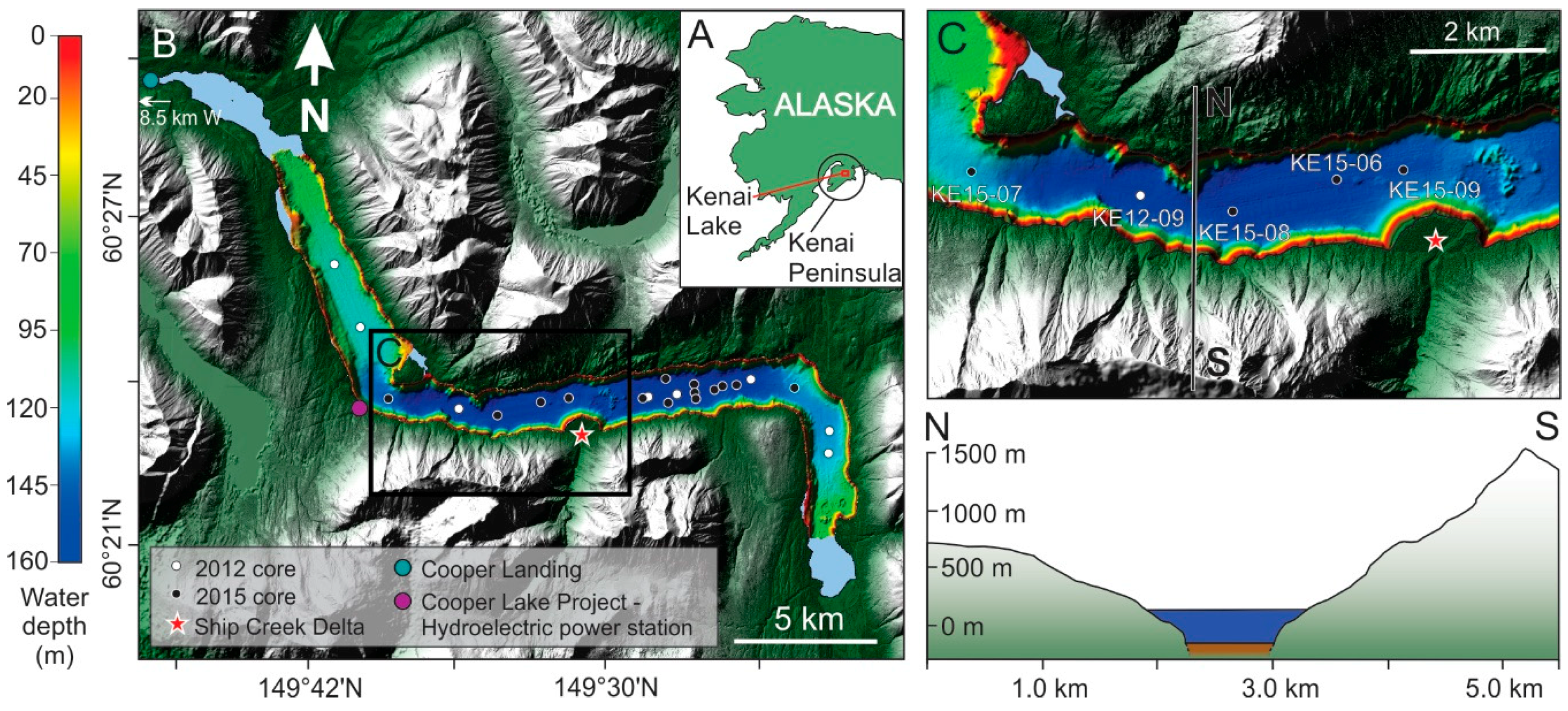
2. Setting

Kenai Lake is a proglacial lake located on the Kenai Peninsula, in south-central Alaska (Figure 1). The Kenai Peninsula can be divided into two regions: the northwest side is the relatively flat Kenai Lowland, and the southeast side is rugged and dominated by the Kenai Mountains where Kenai Lake is situated. The topography of both regions was shaped by Quaternary glacial processes. The Cordilleran Ice Sheet covered most of southcentral Alaska during the Last Glacial Maximum, including the area of Kenai Lake [14]. Kenai Lake was formed by glacial scouring of bedrock and is surrounded by steep mountain slopes.

Kenai Lake is a narrow and zigzag-shaped lake, which is 38 km long and covers a surface area of 56 km². The lake is situated 132 m above sea level and has a maximum water depth of 174 m (Figure 1) [14]. The geology of the surrounding mountains was mapped and described [15] as metasedimentary rocks of the Valdez Group (Upper Cretaceous). The mountains south of the lake are higher (1500 m a.s.l.) and steeper (40–45°) than those in the north (600 m a.s.l., 35–40°) (Figure 1). The lake is hydrologically open with the Upper Kenai River, which is the outlet situated on the northwest end of the lake. The Trail River and Snow River, along the east side of the lake, are the main inlets and sources of water and sediment. A smaller inlet is situated at the north side of the lake [13].

The Kenai Peninsula is situated above the Alaska-Aleutian subduction zone, where numerous active volcanoes are present, and earthquakes occur frequently [16]. These earthquakes and volcanic eruptions can result in the deposition of turbidites and tephras in lakes that can then be used as time markers. In Kenai Lake, the 1964 Great Alaska Earthquake (M_W 9.2) triggered deposition of a turbidite [17], which formed the base of the interval that is studied here. Within this interval, Boes et al. [13] suggested that one of the peaks in the magnetic susceptibility curve, taken along a sediment core, is related to the 1989/1990 Redoubt Volcano eruption.

Kenai Lake sediments are composed of clastic varves, representing a couplet of a coarse-grained spring–summer lamina and a fine-grained winter lamina [13,18]. Boes et al. [13] observed internal laminations in some varves that could be mistaken for a new varve year. These laminations were interpreted to be related to flood events in the late summer or to spring melting of large amounts of snow/ice in a short period.

3. Materials and Methods

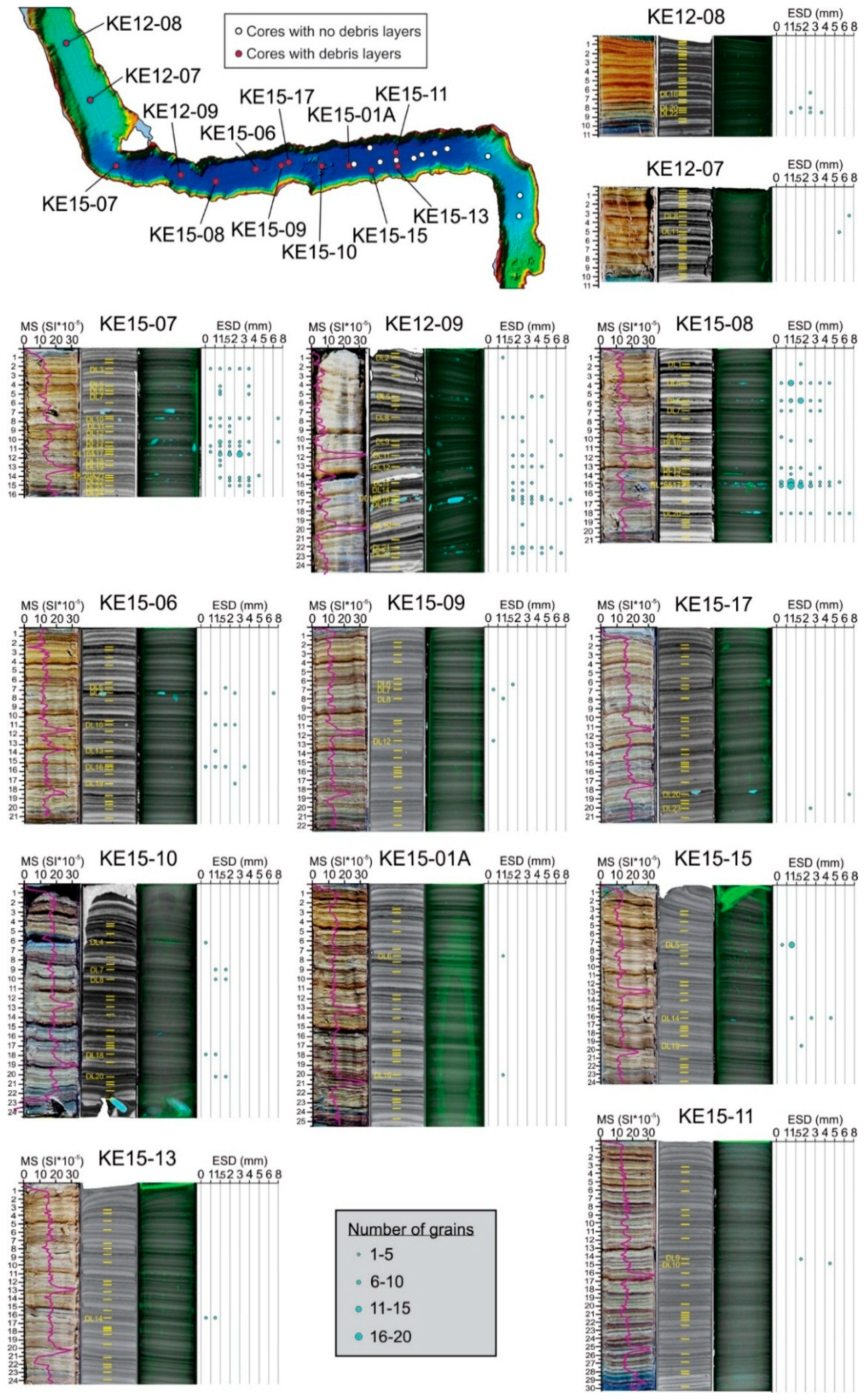
3.1. Multibeam Data, Core Collection and Core Analysis

Multibeam bathymetry data for Kenai Lake were collected in the summer of 2015 using an ELAC SeaBeam 1050 system (ELAC Nautik GmbH, Kiel, Germany). This sonar system has two 50 kHz transducer arrays and a 120° swath angle. Roll, pitch, and heave were corrected by an IXSEA Octans 3000 motion sensor (iXBlue, Cedex, France). CTD measurements (conductivity, temperature and depth) at the lake surface were carried out with a Valeport Modus CTD. A CastAway CTD and a Sea and Sun Technology CTD 48M were used for sound velocity profiles, measured several times each day. The echosounder was controlled by ELAC HydroStar software, which also served as an interface for external sensors that acquired hydrographic information. Processing of the bathymetric data was done with HDPedit (ELAC Nautik GmbH, Kiel, Germany)(outlier cleaning), HDPpost (ELAC Nautik GmbH, Kiel, Germany) (correcting of sound velocity profiles) and IVS 3D Fledermaus™ (QPS B.V., Zeist, The Netherlands) (detailed ping editing). The final high-resolution bathymetry map has a 9-m-grid spacing and a vertical accuracy of a few decimeters.

A total of 27 sediment cores were retrieved during the summer from Kenai Lake using a gravity corer with hammering extension; 9 in 2012 and 18 in 2015. After shipping to Belgium, the cores were split at Ghent University, the working halves were described macroscopically, and geophysical parameters were logged at 0.2 cm resolution using the Geotek Multi-Sensor Core Logger (Geotek Ltd, Northamptonshire, United Kingdom) (MSCL). The MSCL is equipped with a Cs gamma source and detector to calculate gamma density, a Konica Minolta CM-2600d spectrophotometer (Konica Minolta Sensing Americas Inc, Ramsey, New Jersey) to analyze colour spectra and a Bartington MS2E point sensor (Barington Instruments Ltd, Oxon, United Kingdom) to measure magnetic susceptibility. Photographs of the split core surfaces were acquired using the line scan camera mounted on the MSCL.

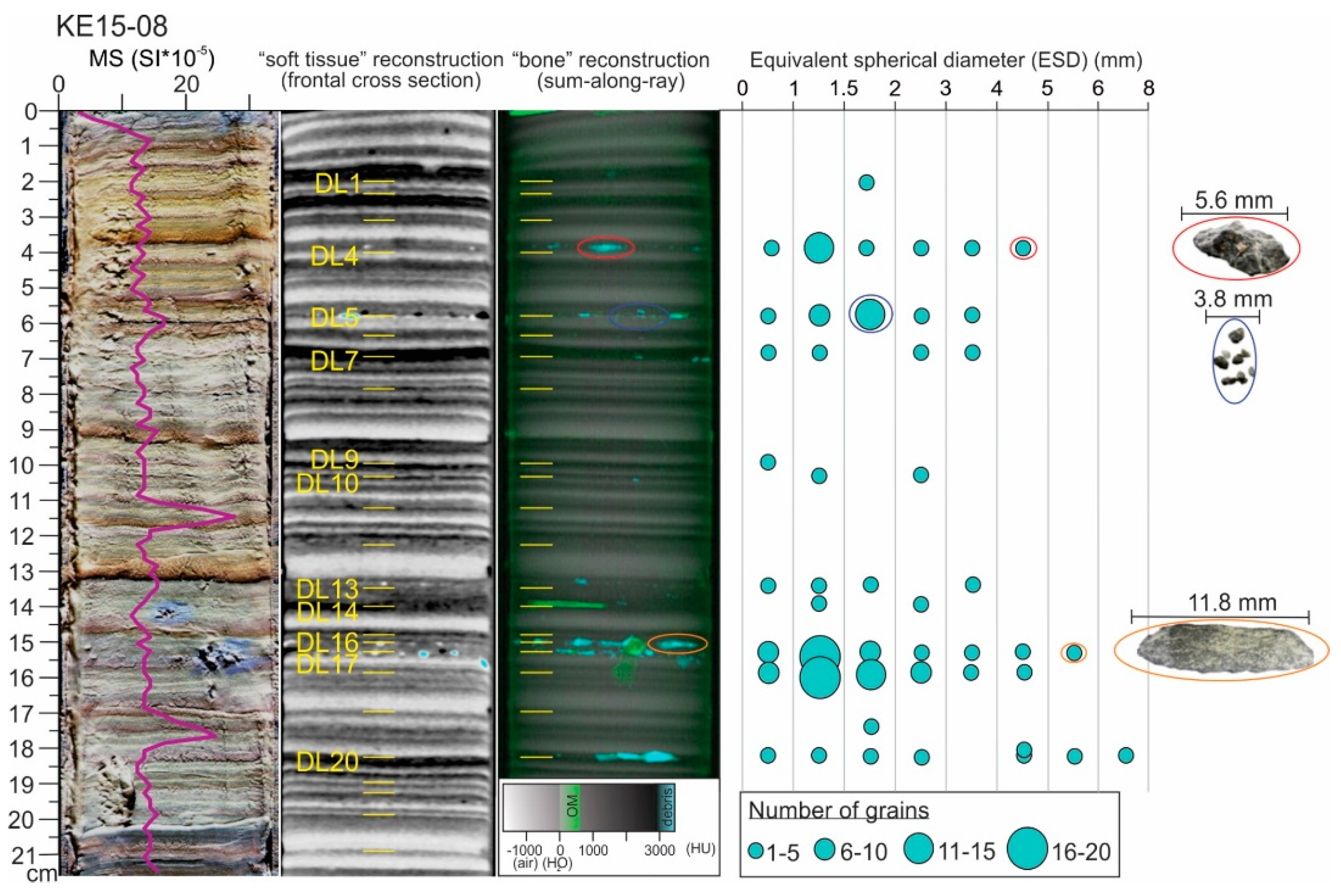
3.2. Core Scanning and Debris Detection

All cores were imaged with a medical X-ray computed tomography scanner (Siemens SOMATOM Definition Flash (Siemens Healthineers, Erlangen, Germany) at the Ghent University Hospital. The scanner was employed at 120 kV, an effective mAs of 200 and a pitch of 0.45. The helical scans were reconstructed using two different protocols. A “soft tissue” reconstruction produced smoother images that have a relatively strong contrast between sediments with low X-ray attenuation. They were used to image the varves in the cores. The “bone” reconstruction produces sharper (but more noisy) images, creating sharp boundaries between objects that have a highly contrasting X-ray attenuation. They were used to image and analyse the medium to coarse sand and gravel in the muddy matrix.

The 2012 cores were split before scanning; while those collected in 2015 were scanned as whole cores. The reconstructed DICOM (Digital Imaging and Communications in Medicine) images have a resolution of 0.15 mm/pixel and a thickness of 0.6 mm and were stacked to create a 3D volume. The step size between consecutive images was 0.6 mm for the 2012 cores, but 0.3 mm for the 2015 cores. Consecutive images of the latter, thus, overlap 50%. The resulting voxel volumes are ~0.014 and ~0.007 mm³ for 2012 and 2015 cores, respectively. The stacks were imported in VG Studio (2.2) for visualisation and were converted to tiff images in ImageJ (64-bit Java 1.6.0_24; [20]). The tiff images of each core were uploaded in Octopus Analysis (formerly known as Morpho+) [21]. This software allows a 3D-analysis of the cores and the segmentation and isolation of groups of voxels, which represent sand or gravel, based on their specific Hounsfield Units (HU), i.e., characteristic grey values which are related to their specific X-ray attenuation [12,22]. A dual threshold of 2200 to 2250 HU in the 2015 cores and 2350 to 2400 HU in the 2012 cores was used to select and isolate sand or gravel. The higher threshold values for the 2012 cores were determined by comparing the HU histograms and are the result of the drier state of these split cores compared to the closed 2015 cores. For each isolated group of voxels (i.e., sand or gravel grains), the equivalent spherical diameter (ESD) was calculated. The ESD represents the diameter of an irregular shaped object calculated from a sphere with the same volume as the aspheric particle [23]. The minimal grain diameter that theoretically can be distinguished (i.e., ~0.24 mm) is affected by the minimal voxel volume of the CT-images (i.e., ~0.007 mm³). Following Nesje et al. and Vasskog et al. [7,10], we refer to the particles with an ESD larger than 0.25 mm (medium sand) as debris particles. For each core, we analyzed both the number of particles present and the ESD of each individual isolated particle (Figure 2). The ESD of the debris particles was used to study their average grain size. The number of particles found in each layer represents a minimum, as some grains are too small or are located too close to the core liner, which makes it very difficult or impossible to isolate this group of voxels. The stratigraphic position of each grain was linked to a particular varve. Based on the CT-images and the results of the grain-size analysis of the debris, two cores (i.e., KE15-07 and KE15-08) were selected for sampling of grains of different sizes (Figure 2). These fragments were visually examined to identify the rock type, which can help to assign a possible source region to the debris.

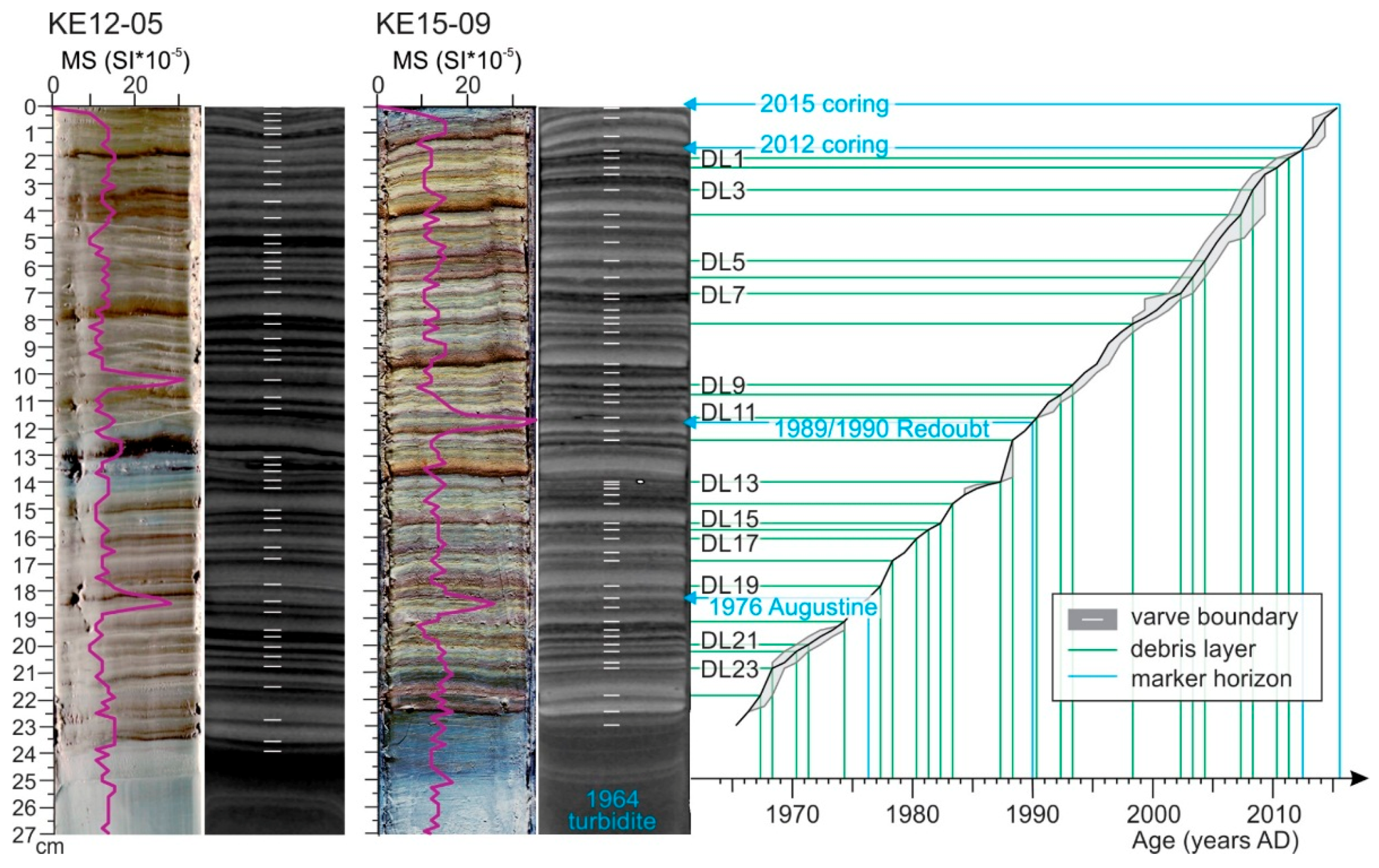
3.3. Core Correlation, Varve and Tephra Chronology

The cores containing debris were correlated by marker horizons and the sequences of varves present in each core. Varves containing debris were marked as debris laminae (DL) followed by the number of the layer, starting at the sediment–water interface and counting downwards to the top of the turbidite deposited in response to strong shaking during the 1964 earthquake [17]. Dating of the different debris laminae was based on the varve chronology, corroborated by tephra marker beds. The different varves are formed in varve years (VY), which start at the beginning of the melting season (spring) and end at the end of winter [13,18], e.g., VY2014 starts approximately in May 2014 and ends in April 2015.

The varve chronology of the different cores is based on varve counting and chronology by Boes et al. [13]. This original chronology is correlated to historical volcanic eruptions based on newly acquired glass geochemistry data from two cryptotephras indicated by sharp MS peaks (Figure 2). The uncertainty of the varve chronology between marker horizons was calculated using the presence of uncertain varves that were retained for the chronology (a potential “erroneous” varve [17]) and uncertain varves that were not used in the chronology (a potential “missing” varve [17]). From each marker horizon downward, minimum and maximum ages were calculated by summing “erroneous” and “missing” varves, respectively. From each marker horizon upward, minimum and maximum ages were calculated by summing “missing” and “erroneous” varves, respectively. As a result, each lamina receives two minimum and two maximum ages (i.e., one relative to both the nearest marker horizon above and below). From those, the minimum and maximum ages representing the lowest uncertainty were retained.

Cryptotephra samples were treated with 35% hydrogen peroxide to remove organic material and washed through a 20 μm sieve. Glass was separated using LST (lithium heteropolytungstate) heavy liquid at ~2.45 g/cm³ and mounted in acrylic pucks using SpeciFix-20 epoxy. All analyses were by wavelength-dispersive spectrometry (WDS) on a JEOL 8900 SuperProbe (JEOL USA Inc, Peabody, Massachusetts) at the University of Alberta using 15 KeV, 6 nA current and 5 μm beam. The software ‘Probe for EPMA’ (Probe Software Inc, Eugene, Oregon) was used to apply time-dependent intensity corrections for Na loss induced by the smaller beam size [24]. Two natural glasses, Lipari obsidian (ID3506) and Old Crow tephra, were analyzed before and after the samples to track calibration and the quality of analyses.

3.4. Satellite Image Analysis

Satellite images were used to visually verify the occurrence of snow avalanches in winters over the period 2004 to 2014. The location and timing of these avalanches were compared to the ages of debris laminae found in the lake sediments. Satellite images from Landsat 5,7,8 /Copernicus (Property Google—DigitalGlobe 15–30 m resolution, 14 April 2004, 17 April 2011), Pleiades (0.5 m resolution, 2 April 2012), QuickBird (0.6 m resolution, 23 March 2014) and WorldView-1 (0.5 m resolution, 28 April 2008) were used to study the frozen conditions of Kenai Lake towards the end of the winter season (March–April). For other years, we were not able to locate satellite images with sufficient resolution.

3.5. Climate Data

The Alaska Climate Research Center provided climate data for the period 1963 to 2013 (for winter temperature and snowfall) collected at two stations located near Kenai Lake. These two stations were Cooper Lake Project (60°23’N, 149°41’W, 182 m above sea level) and Cooper Landing (60°29’N, 149°58’W, 105 m above sea level) (Figure 1).

4. Results

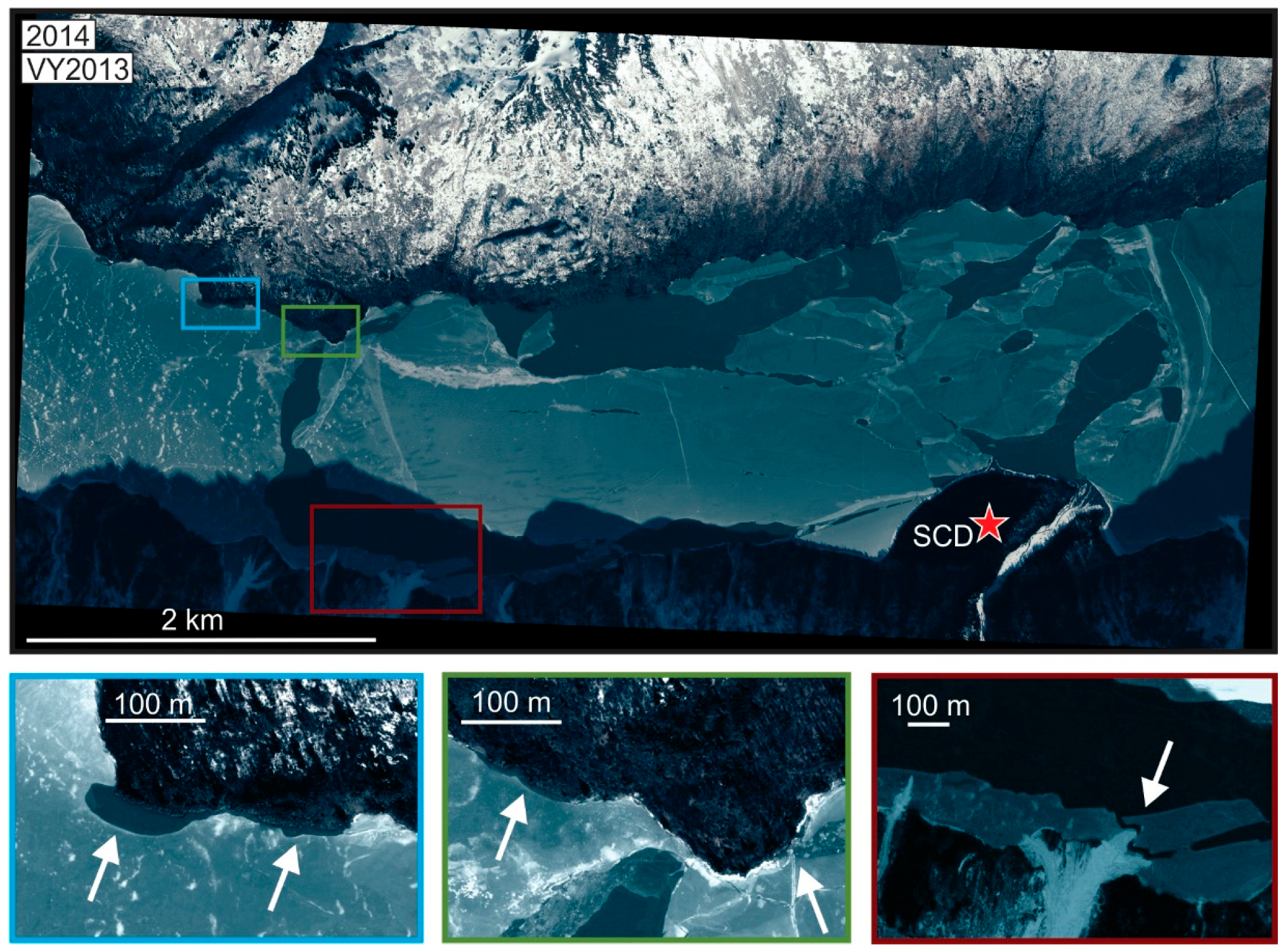
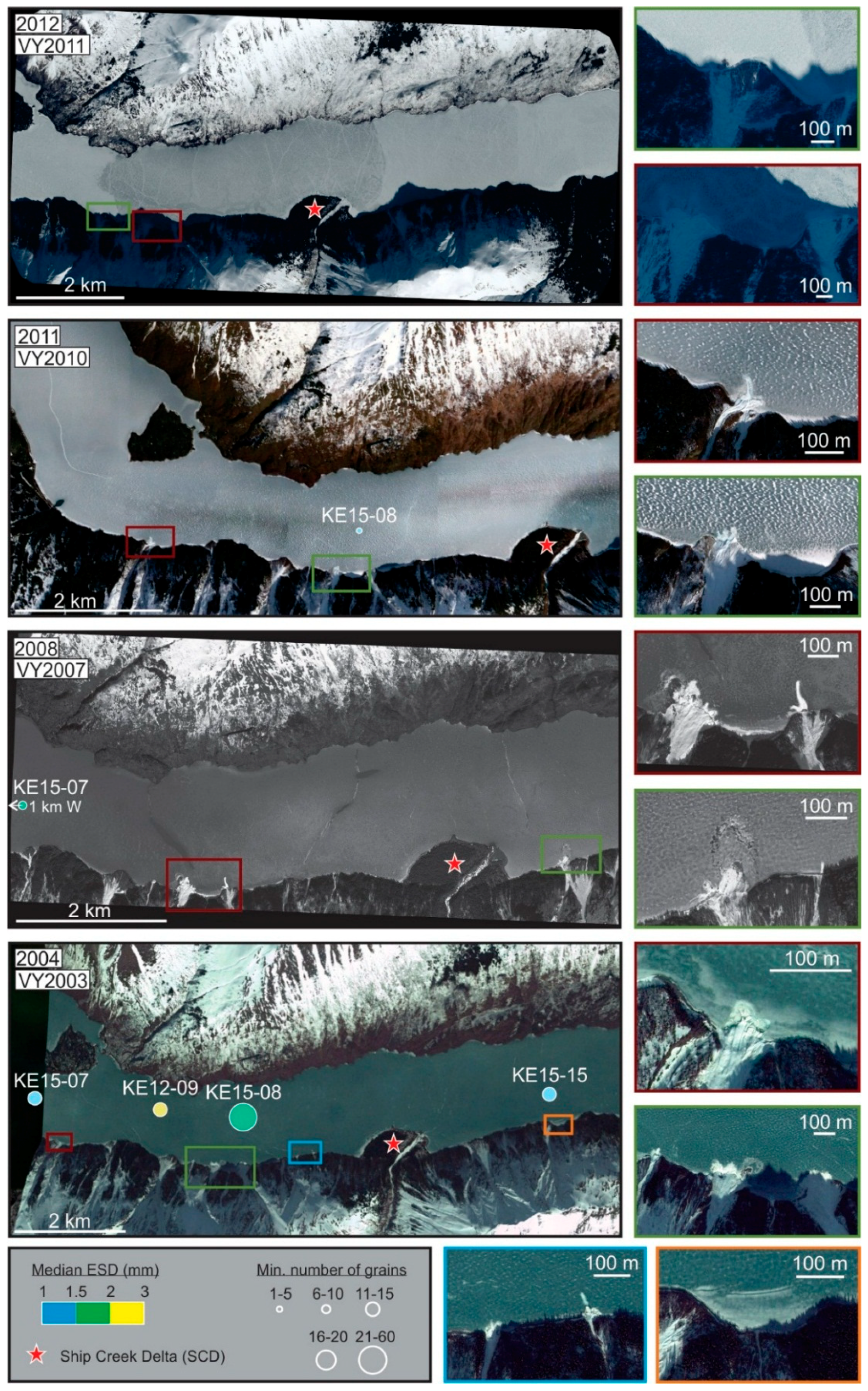
4.1. Avalanches on Satellite Images

We observed snow-avalanche deposits on the five available satellite images over the period 2004 to 2014 along the south shore of the central basin of Kenai Lake (Figure 3 and Figure 4). The majority of these can be found between the Hydroelectric Power Station (HPS) and the Ship Creek Delta (SCD) (Figure 1), while a few are situated east of Ship Creek Delta. We refer to these places as the western part and the eastern part of the central basin, respectively. In the captions of Figure 3 and Figure 4, we describe the distribution and transport processes of observed avalanche deposits based on satellite images.

4.2. Bathymetry

The bathymetry of Kenai Lake can be characterized as a flat basin plain bordered by steep slopes that are typically 30 to 45°, and locally, as steep as 70° (Figure 1). Deltas have average slopes of 20 to 30°. At the foot of major deltas, the hummocky mounds are probably deposits from delta failures.

4.3. Core Sedimentology

Most sediments in Kenai Lake are clastic varves (see 2. Setting; [13]). The varves have a grain-size distribution ranging from clay to silt [13] and form the matrix in which the coarse debris was deposited. The post-1964 sedimentary sequence thickens from the west to the east. The considerably thicker sedimentary sequence in the central and eastern basins (21 to 30 cm) compared to the western basin (11 to 16 cm) (Figure 5) is a result of the river inlets, which are situated in the eastern and central part of the lake. These rivers bring sediment into the lake, which is deposited primarily near the inlets. Within the central basin, the thickness is relatively constant, with slightly thicker (max. 5 cm) sequences on delta-proximal locations.

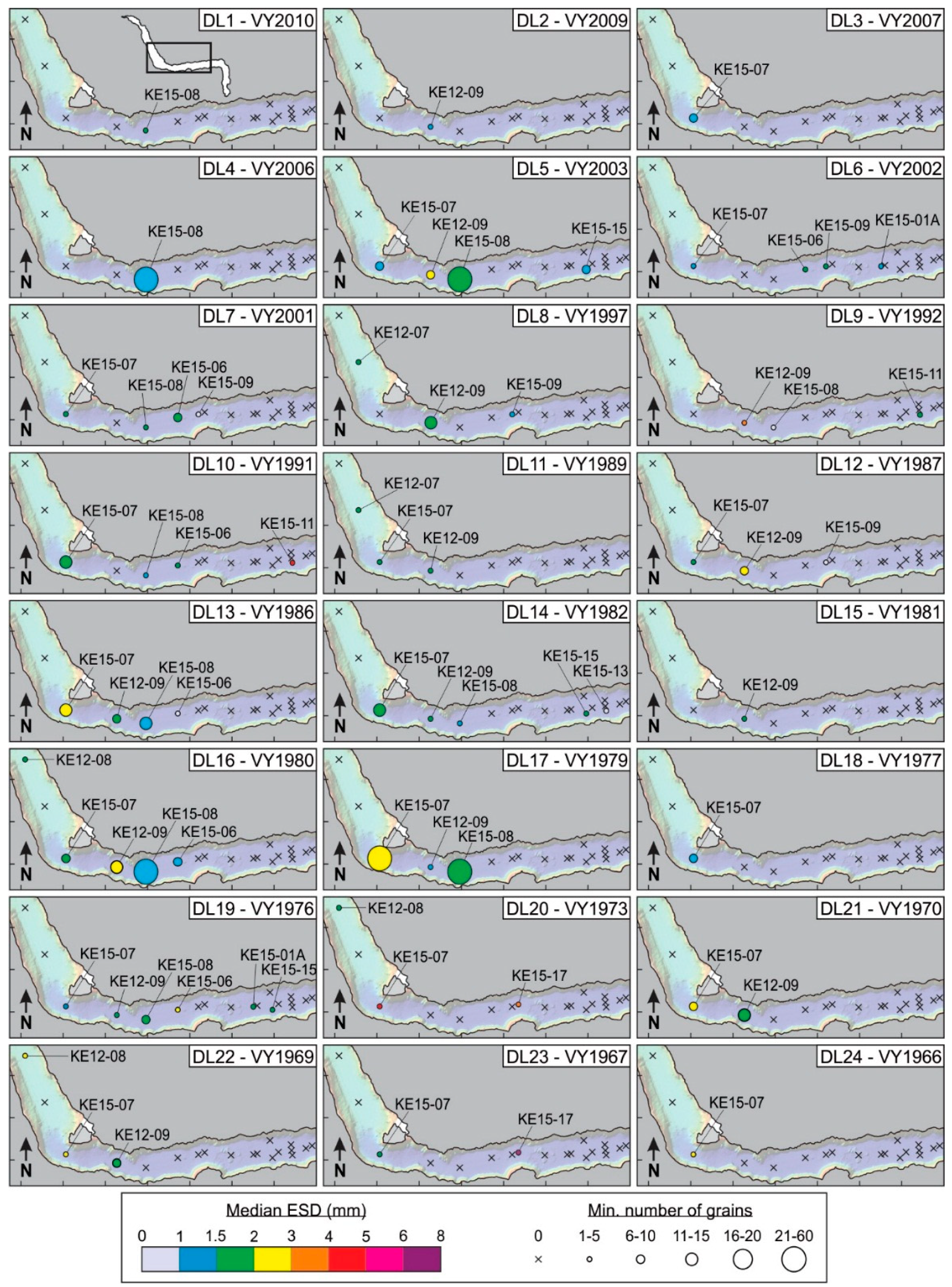
4.3.1. Debris Laminae

Debris was found in three of the nine cores taken in 2012 (i.e., KE12-07, KE12-08, and KE12-09) and in 11 out of 18 2015-cores (i.e., KE15-01A, KE15-01B, KE15-06, KE15-07, KE15-08, KE15-09, KE15-10, KE15-11, KE15-13, KE15-15, and KE15-17) (Figure 5). In each core, the debris was found in, or just above, the winter lamina of a varve (Figure 2).

Twenty-four debris laminae were identified in the 14 debris-containing cores; most of the debris laminae were found in cores from the southern part of the western basin and in the western part of the central basin (Figure 5 and Figure 6). Core KE15-07, located at the western end of the central basin, records 20 of the 24 debris laminae (Figure 5). The equivalent spherical diameters (ESD) of the debris grains range from 0.35 mm to 12.30 mm. In general, debris consists of very coarse sand to fine gravel. An overview of the physical properties (mean, median, maximum and minimum grain size) of all the grains found in each debris lamina is presented in

Table 1. Characteristics of debris laminae in the cores, their ages and physical properties of the grains (DL = debris lamina, ESD = equivalent spherical diameter).

Name	Varve Year	Best Age (years AD)	Min Age (years AD)	Max Age (years AD)	Number of Cores in which DL is Present	Total Number of Grains in DL	Mean ESD (mm)	Median ESD (mm)	Max ESD (mm)	Min ESD (mm)
DL1	2010	2011.3	2011.3	2010.3	1	1	1.75	1.75	1.75	1.75
DL2	2009	2010.3	2010.3	2009.3	1	1	1.50	1.50	1.50	1.50
DL3	2007	2008.3	2009.3	2007.3	1	9	1.70	1.68	3.04	0.98
DL4	2006	2007.3	2009.3	2006.3	2	24	1.49	1.17	5.00	0.74
DL5	2003	2004.3	2005.3	2003.3	4	53	1.87	1.52	4.86	0.60
DL6	2002	2003.3	2004.3	2002.3	4	5	1.55	1.57	1.81	1.21
DL7	2001	2002.3	2003.3	2001.3	5	16	2.23	2.15	7.17	0.56
DL8	1997	1998.3	1999.3	1998.3	4	9	3.00	2.51	8.33	1.29
DL9	1992	1993.3	1990.3	1993.3	3	6	2.05	1.29	5.78	0.74
DL10	1991	1992.3	1993.3	1992.3	4	21	2.05	1.69	6.03	0.89
DL11	1989	1990.3	1990.3	1990.3	3	11	2.74	1.90	7.50	0.91
DL12	1987	1988.3	1988.3	1988.3	3	11	2.52	2.06	5.00	0.78
DL13	1986	1987.3	1987.3	1987.3	4	37	1.95	1.70	7.05	0.69
DL14	1982	1983.3	1983.3	1983.3	5	25	1.95	1.61	7.70	0.35
DL15	1981	1982.3	1982.3	1982.3	1	5	2.62	2.51	4.03	1.51
DL16	1980	1981.3	1981.3	1981.3	4	73	2.15	1.51	15.50	0.65
DL17	1979	1980.3	1980.3	1980.3	3	95	1.87	1.64	7.83	0.80
DL18	1977	1978.3	1978.3	1978.3	2	8	1.47	1.49	1.98	1.00
DL19	1976	1977.3	1977.3	1977.3	6	15	2.48	1.62	7.58	0.99
DL20	1973	1974.3	1974.3	1974.3	3	4	4.20	3.60	7.93	1.68
DL21	1970	1971.3	1972.3	1970.3	2	20	2.59	2.23	5.28	1.13
DL22	1969	1970.3	1971.3	1969.3	3	17	2.89	2.64	6.26	1.01
DL23	1967	1968.3	1969.3	1968.3	2	5	2.23	1.90	2.99	1.52
DL24	1966	1967.3	1968.3	1967.3	1	1	2.23	2.23	2.23	2.23

.

Debris was only sampled in cores KE15-07 and KE15-08. The debris in both cores generally consists of angular, often flattened, grains with a dark gray colour and shiny surface, sometimes accompanied by organic detritus. In debris lamina 4 from core KE15-08 (at 3.5 to 4 cm from the top of the core) one dark grey, angular pebble, 0.6 cm long with a flattened shape and a flaky surface texture was present, which was accompanied by smaller sand grains (<1 mm) (Figure 2). In debris lamina 5 (at 5 to 6 cm from the top) we found sand grains with a diameter up to 1 mm. Whereas most of the grains are angular and dark grey, some grains were more rounded and vary in colour between yellow and dark grey. Organic material, such as wood chips, was found in the matrix, together with debris particles. In debris lamina 16 at a depth of 14.5 to 15.5 cm from the top, sand grains similar to those in debris lamina 4 and 5 were found. In addition to the small grains, we found a 1.2-cm-long, dark grey, angular pebble.

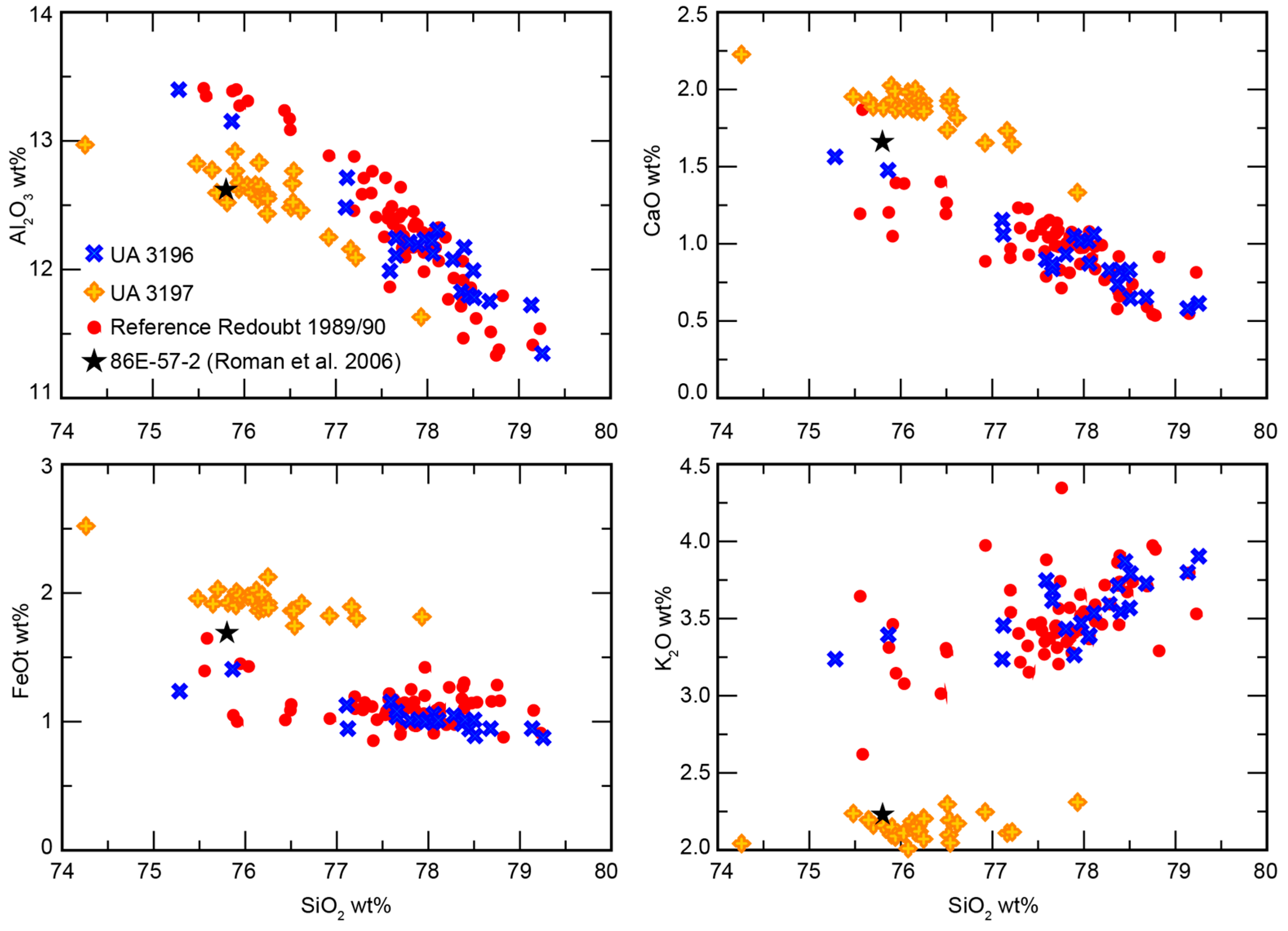
4.3.2. Tephra Geochemistry

The two cryptotephras, which were identified by their magnetic susceptibility peaks, occur throughout the lake (Figure 5). They were sampled in core KE12-05 at a depth of 10.0 to 10.4 cm (UA3196) and 18.7 to 19.0 cm (UA3197). Glass geochemical analyses are shown in

Table 2. Averages and standard deviations (std) of major-element glass geochemistry of tephra samples.

Sample	SiO2	TiO2	Al2O3	FeOt1	MnO	MgO	CaO	Na2O	K2O	Cl	H2Odiff2	n3
UA3196	77.58	0.27	12.30	1.12	0.06	0.20	0.99	3.85	3.52	0.12	1.27	24
std	1.42	0.06	0.63	0.33	0.02	0.11	0.34	0.31	0.23	0.04	1.26
UA3197	76.20	0.37	12.57	1.93	0.05	0.42	1.88	4.10	2.21	0.33	1.62	29
std	0.65	0.05	0.27	0.14	0.02	0.06	0.15	0.32	0.36	0.03	1.02

¹ Fe is presented as total FeO (FeOt); ² All analyses are normalized to 100% on a water-free basis; ³ n = number of analyses.

. Both samples have high SiO₂ values. However, sample UA3197 is characterized by relatively high CaO and FeOt, and low K₂O values compared to sample UA3196. All individual glass shard analyses, including standards, are available as supplementary materials (Table S1).

5. Discussion

5.1. Chronology

Glass geochemical analyses show that the upper tephra (UA 3196) correlates to the 1989/90 Redoubt Volcano eruption (Figure 7). This tephra is a regional marker and present as a cryptotephra across a large portion of Yukon and Alaska [25]. The second tephra (UA 3197) was, based on its stratigraphic position, presumed to be sourced from the large 1976 eruption of Augustine Volcano with a Volcanic Explosivity Index (VEI) of 4. While we do not have access to reference material from this particular event for comparison, existing data support this correlation. Overall, the glass geochemical characteristics of this sample fall within the variability displayed by historic and pre-historic Augustine tephras, with distinctive traits, such as low K₂O (<2.5 wt%) and higher Cl (~0.25–0.35) contents (e.g., [26,27]). The most similar material are several pumice analyses presented by Roman et al. [27] from the 1986 eruption of Augustine Volcano (Figure 7). The average of their analyses plot with, or very near, UA 3197.

The 1976 eruption of Augustine Volcano had several phases over four months from January until April, including a large event on January 24 where column heights reached ~14,000 m a.s.l., and ashfall was reported on Kenai Peninsula and as far as Anchorage (e.g., [28,29]). The Alaska Volcano Observatory’s comprehensive database of eruptions shows that only four other volcanoes had eruptions around this time: Shishalden, Pavlof, Akutan, and the Ukinrek Maars. It is very unlikely that ash from Akutan, Shishalden, and Pavlof would have reached this region; the most proximal of these three volcanoes (Pavlof) is 750 km from Kenai Peninsula, all eruptions had a VEI ≤2 with column heights not reaching above 2500 m a.s.l., and no ash was reported beyond the immediate region. Additionally, the eruptions appear to have been largely strombolian involving lava flows, suggesting that products would not have been rhyolitic as erupted at Augustine. The only other large event around this time were the eruptions of the Ukinrek Maars in 1977 (VEI 3) that ejected ash over a wide region, reaching Kodiak Island, south of Kenai Peninsula. However, these were basaltic eruptions (e.g., [30,31]).

We use the two tephra ages to revise the original varve chronology of Kenai Lake by Boes et al. [13] (Figure 8). From the top of the core until the appearance of the first tephra layer (UA3196) the original chronology is unchanged. Only in the lower part of the studied interval, from UA3196 to the 1964-turbidite, the original chronology underwent minor modification. The early 1976 Augustine provenance of tephra UA3197 allows us to attribute the varve with the tephra to varve year 1975. We also know that the position of the 1964-turbidite in the cores was triggered in March 1964 by the M_w 9.2 Great Alaska earthquake [16]. As it likely takes several months, or even longer, to deposit the fine-grained cap of the turbidite [32], the first varve following the turbidite would have been deposited in varve year 1965. The original varve chronology was lacking one varve in between the two absolute time markers (i.e., the 1964 turbidite and the 1976 Augustine tephra), and we, therefore, reinterpret as two varves the multipulsed varve in which debris layer 23 is located (Figure 8).

5.2. Evidence for Snow Avalanches as the Origin of Coarse Debris

The mountains surrounding the lake are the source area of the debris, and the angularity of the fragments indicates that snow avalanches are likely the initial mechanism responsible for the erosion and transport of sand and gravel onto the lake ice. The metasedimentary rocks in the catchment match the rock type of the large clasts from cores KE15-07 and KE15-08. We infer that during spring melting of the lake ice, sediment transported by snow avalanches is then distributed across much of the lake by drifting ice pans.

Satellite images of the Kenai Lake area provide more evidence for snow avalanches as the primary mechanism to bring debris to the lake. Images taken at the end of the winter season (March–April) show snow-avalanche deposits as clearly visible on the frozen lake. However, they do not reach the middle of the lake, where the cores were taken. We explain the deposition of debris in the middle of the lake by the melting processes of the ice in the spring. On the 2014 satellite image (Figure 3), ice along the north coast of the lake starts melting first, and the ice starts cracking across the lake. Cracking of the ice results in ice floes on the lake water, which carry debris initially deposited on the ice near the shore and deliver it to the centre of the lake [9]. The outlet of the lake, the Kenai River, is situated at the northwest end of the lake, and in combination with the predominant easterly wind direction in the months April and May [33], we infer that ice floes would drift westward towards the outlet. Evidence of this westward drift is found in core KE15-07, which contains the most debris laminae of all the cores and is located west of the zone with most snow-avalanche deposits (Figure 5). The other cores with debris were all taken near to, or west of, the source areas, while no debris was found in the cores east of the source areas. Other potential transport mechanisms, such as transport by birds or floating logs, would all be from initially fluvially transported sediment, and the grains would likely be rounded. One would expect a more random distribution of the debris both in time and in space if such a process was responsible for the observed debris. Turbidity currents resulting from onshore rock failure can transport angular grains. We rule out this transport mechanism because the debris particles in the Kenai Lake sediment cores occur typically in the muddy matrix of the varved sediments and not in graded turbidites.

A similar process was proposed to explain the presence of debris in Norwegian [11], Canadian [9], and French lakes [34]. Seierstad et al. [11] observed a dirty snow avalanche, indicating that a significant amount of debris and organic material together with snow and ice was transported by avalanches onto the frozen lake. The process was first described by Luckman [9] who observed it on Canadian lakes in the 1970s. Later, Seierstad et al., Nesje et al., Vasskog et al., and Fouinat et al. [7,10,11,34] explained the distribution of snow-avalanche debris across a lake by the same process. The snow-avalanche debris gets deposited in the spring melting season, at the transition to a new varve year. The coarse particles sink into the fine-grained top of the previous varve. This can be observed in the X-ray CT images (Figure 2 and Figure 5), where all debris particles are situated in the black winter lamina.

5.3. Snow Avalanche Record

5.3.1. Variable Avalanche Extent on Satellite Images

The satellite images from Kenai Lake in the month of April over several years show that snow avalanches were deposited on the lake almost every year. However, not every varve contains debris. In years with large snow-avalanche deposits, such as 2004, a debris deposit is present in several cores throughout the lake, whereas smaller avalanche deposits, like in the years 2012 and 2014, are not always represented by debris in one of the sediment cores (Figure 4). The satellite images of these years show that the avalanche deposits are not reaching as far onto the lake ice as they do in other years, and it is possible that during cracking of the ice along the shore, part of the deposit already ends up near the shore [10]. As a result, these snow avalanches are not recorded in the cores taken in the middle of the lake. The 2014 satellite image (Figure 3) shows that ice cracks form around some of the avalanche deposits along the south shore. It is likely that these deposits will not detach from the shoreline, resulting in deposition of the debris on the slopes. Furthermore, depending on which shore of a lake (i.e., shady or sunny—the northern shoreline of Kenai Lake receives more sunlight every day then the south shore, thus lake ice will melt first along the north shore) a snow avalanche is deposited, the debris may or may not get redistributed by drifting ice across the lake.

5.3.2. Natural Factors Affecting the Lacustrine Snow-Avalanche Records

The chance that a snow avalanche is recorded in the lacustrine sediments depends on several factors. The avalanche needs to be large enough and have a sufficiently high velocity so that it spreads far enough onto the ice when it reaches the lake. When an avalanche is too large, it could possibly break the ice when it hits the lake [34], even though this process was not observed on any of the satellite images of Kenai Lake. This process is more likely to happen in the beginning or towards the end of the freezing season as lake ice is still/already thinner and less stable. Only dirty snow avalanches, i.e., avalanches that contain organic material and coarse rock grains, will be recorded in the lake sediments as we can distinguish the coarse avalanche material from the fine lake sediments [9]. In addition to the physical characteristics of the snow avalanche, the melting processes of the lake ice also play an important role in the recording of avalanche deposits in the lake. Depending on where the cracks in the ice form, on wind direction and lake currents [9], the avalanche debris will be deposited at different places across the lake.

Apart from avalanches themselves, the physical characteristics of the lake will influence the record. For example, Lake Lauvitel, studied by Fouinat et al. [6,34] using X-ray CT, is about 130 times smaller than Kenai Lake, which strongly affects the redistribution of avalanche debris. In a smaller lake, such as Lake Lauvitel, there is an increased probability that the snow-avalanche deposits will be spread over most of the lake, thereby increasing the likelihood that a single core will contain a complete record of past avalanches reaching the frozen lake [e.g., 34]. The larger size of Kenai Lake, however, inhibits snow avalanches from reaching the central part of the lake and debris redistribution is, thus, strongly affected by the pathway of drifting ice floes during the melting season. In such large lakes, it is, thus, crucial to conduct a calibration study, such as this one, where multiple short cores are used to map the deposits (Figure 6) and determine the optimal coring locations for a complete record (it should be noted that the cores in this study were not targeted for a snow-avalanche reconstruction). In Kenai Lake, this is the western part of the central basin, in front and to the west of the main avalanche tracks. Cores KE15-07, KE12-09, and KE15-08 contain 18, 14, and 11 out of 24 debris layers, respectively, and combined they contain all 24 recorded debris layers (Figure 5). In the eastern part of the central basin, primarily cores close to the shores contain snow-avalanche debris (e.g., KE15-13 and KE15-15; Figure 5). Such relatively near-shore locations may, thus, contain a more complete avalanche record than cores in the center of the deep basin. Finally, while for a small lake it may be easier to reconstruct a more complete snow avalanche history of a few avalanche tracks, a large lake has the advantage to potentially record avalanches from a larger number of tracks, providing a regional avalanche record.

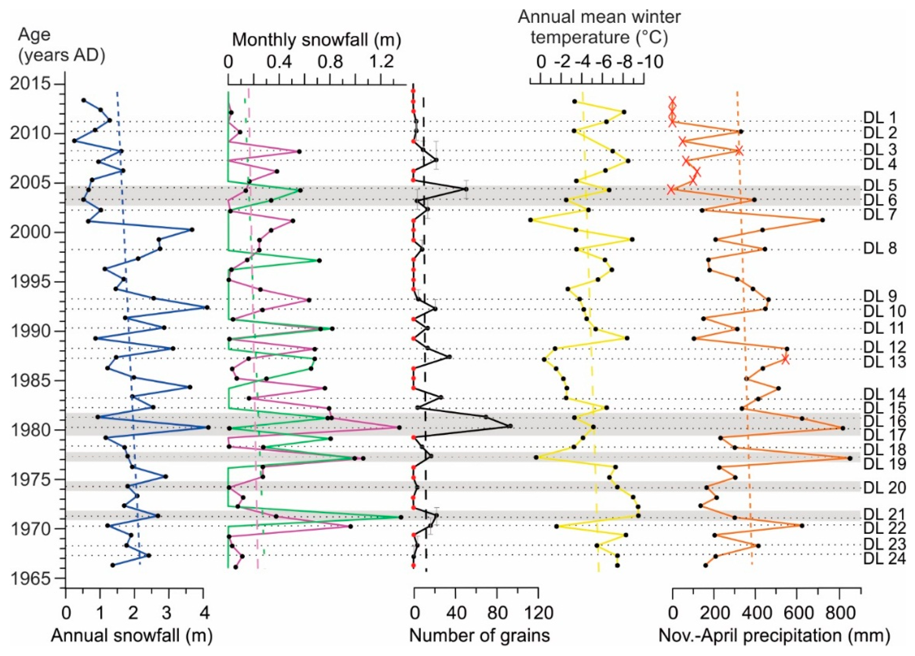
5.3.3. Comparison of Snow Avalanche and Climate Records

Climate variables, such as mean, maximum and minimum monthly temperature and monthly snowfall (data from the Alaska Climate Research Center), were compared to grain-size distributions and the number of grains from all debris laminae. Baggi et al. [35] suggested that a snowpack is weakened by 1) gradual warming of the snowpack to 0 °C, 2) loss of strength by water infiltration into the snowpack, and 3) overload of the (wet) snowpack by precipitation. These weakening factors of the snowpack could trigger a wet-snow avalanche. In Kenai Lake, we can link the presence of a debris lamina to a varve year where there was snow precipitation in a month with a mean temperature above 0 °C (Figure 9). For example, in 1980 (varve year 1979) a high amount of snow fell in months with a mean temperature above 0 °C and in this varve year, DL17—the debris laminae with most grains of the record—was deposited.

Snow avalanches, specifically slab avalanches, can also initiate from weak bonding of snow above melt–freeze crusts. These crusts typically form during a warmer (melting) period followed by a colder (freezing) period. When fresh snow precipitates on the crust, it will fail to bond to it and can release slab avalanches [36,37,38]. Our climate data show a link between warmer temperatures in January–February and the presence of debris laminae in that varve year. For example: in 2003 (varve year 2002), when DL6 was deposited, the months of December and January had a mean monthly temperature of −3.4 and −3.2 °C, respectively. In February the mean temperature increased to 0.6 °C and decreased again in March to −4.1 °C. In addition to a drop in temperature, March showed a high amount of snow precipitation. The climate data indicate a melt–freeze crust formed in February-March and that, with increased snow in March, the snowpack became unstable and triggered slab-avalanches. A similar series of events occurred in 2004 (varve year 2003), resulting in DL5, during the year in which most avalanche deposits were observed on the satellite imagery (Figure 3 and Figure 4). We did not identify any relationship among the mean annual winter temperature (Figure 9; yellow plot) or the total annual snowfall (Figure 9; blue plot) and the appearance of debris laminae in lake cores (Figure 9; black plot).

Based on the two mechanisms for avalanche formation, it is possible to link most of the debris laminae to the climate data. However, several other factors can play a role in the triggering of snow avalanches, such as daily temperature and snowfall, wind strength and direction, and snowpack characteristics. The climate data show several years with good snow-avalanche conditions, but during which no debris was found in the lake sediments, as well as years in which debris was found, but weather conditions did not match with snow-avalanche conditions. This may be due to insufficient climate data, coring location, ice conditions, or the redistribution process of the avalanche debris by drifting ice floes.

In the 50-year period studied (1965–2015), linear fits of temperature and snow/precipitation plots show decreasing trends. The linear fit of the number of debris laminae, and, thus, the recorded snow avalanches in the lake, also shows a minor decreasing trend. This may be the result of fewer snow avalanches as the amount of snowfall and precipitation decreased during this period.

6. Conclusions

-

X-ray CT scans of the cores from Kenai Lake show varved lake sediments and help identify coarse sediment laminae, which we infer as snow-avalanche debris, in a non-destructive methodology. We identified 24 debris laminae in 14 cores, with the coarsest and highest number of grains occurring in the western part of the lake. It is the first time that this technique was used on such a large scale for the identification of snow-avalanche debris.

-

We made minor corrections to a previously developed varve chronology using cryptotephras from the 1976 Augustine Volcano eruption and the 1989/90 Redoubt Volcano eruption.

-

Based on the rock type of coarse debris and satellite images of avalanche extent over 10 years, we concluded that snow avalanches emanate from the mountains around the lake, and deposit snow and sediment debris onto the frozen lake surface. In spring, the ice breaks up, and ice floes and pans with snow-avalanche deposits drift westward on the lake (forced by river outflow and prevailing wind directions). When the ice melts, debris is deposited on the lake bottom predominantly in locations westward of where the avalanches reached the lake ice. Debris deposition in the varved sediments allows us to date snow-avalanche events with annual resolution.

-

Comparison of climate data with the debris laminae record shows that snow avalanches tend to occur in months with a mean positive temperature and increased snow fall. Snow avalanches also occur when there is a sudden temperature rise in winter followed by colder temperatures and snow fall.

-

Although the annual debris record is not complete enough to fully reconstruct the regional snow avalanche history, it can be used for decadal reconstructions of past snow-avalanche activity.

-

From 1966 to 2014, less snowfall has resulted in a lowering frequency of snow avalanches.

References

- Colorado Avalanche Information Center. Available online: http://avalanche.state.co.us/accidents/statistics-and-reporting/ (accessed on 17 October 2018).
- Techel, F.; Jarry, F.; Kronthaler, G.; Mitterer, S.; Nairs, P.; Pavšek, M.; Valt, M.; Farms, G. Avalanche fatalities in the European Alps: Long-term trends and statistics. Geogr. Helv. 2016, 71, 147–159. [Google Scholar] [CrossRef]
- Stethem, C.; Jamieson, B.; Schaerer, P. Snow avalanche hazard in Canada—A review. Nat. Hazards 2003, 28, 487–515. [Google Scholar] [CrossRef]
- Ballesteros-Cánovas, J.A.; Trappmann, D.; Madrigal-González, J.; Eckert, N.; Stoffel, M. Climate warming enhances snow avalanche risk in the Western Himalayas. Proc. Natl. Acad. Sci. USA 2018, 115, 3410–3415. [Google Scholar] [CrossRef] [PubMed]
- Butler, D.R.; Malanson, G.P. A History of High-Magnitude Snow Avalanches, Southern Glacier National Park, Montana, USA. Mt. Res. Dev. 1985, 5, 175–182. [Google Scholar] [CrossRef]
- Fouinat, L.; Sabatier, P.; Poulenard, J.; Reyss, J.L.; Montet, X.; Arnaud, F. A new CT scan methodology to characterize a small aggregation gravel clast contained in a soft sediment matrix. Earth Surf. Dyn. 2017, 5, 199–209. [Google Scholar] [CrossRef]
- Nesje, A.; Bakke, J.; Dahl, S.O.; Lie, Ø.; Bøe, A.G. A continuous, high-resolution 8500-yr snow-avalanche record from western Norway. Holocene 2007, 17, 269–277. [Google Scholar] [CrossRef]
- Butler, D.R.; Sawyer, C.F. Dendrogeomorphology and high-magnitude snow avalanches: A review and case study. Nat. Hazards Earth Syst. Sci. 2008, 8, 303–309. [Google Scholar] [CrossRef]
- Luckman, B.H. Drop Stones Resulting from Snow-Avalanche Deposition of Lake Ice. J. Glaciol. 1975, 14, 1–3. [Google Scholar] [CrossRef]
- Vasskog, K.; Nesje, A.; Støren, E.N.; Waldmann, N.; Chapron, E.; Ariztegui, D. A holocene record of snow-avalanche and flood activity reconstructed from a lacustrine sedimentary sequence in Oldevatnet, western Norway. Holocene 2011, 21, 597–614. [Google Scholar] [CrossRef]
- Seierstad, J.; Nesje, A.; Dahl, S.O.; Simonsen, J.R. Holocene glacier fluctuations of Grovabreen and Holocene snow-avalanche activity reconstructed from lake sediments in Grøningstølsvatnet, western Norway. Holocene 2002, 12, 211–222. [Google Scholar] [CrossRef]
- Cnudde, V.; Boone, M.N. High-resolution X-ray computed tomography in geosciences: A review of the current technology and applications. Earth-Sci. Rev. 2013, 123, 1–17. [Google Scholar] [CrossRef]
- Boes, E.; Van Daele, M.; Moernaut, J.; Schmidt, S.; Jensen, B.J.L.; Praet, N.; Kaufman, D.; Haeussler, P.; Loso, M.G.; De Batist, M. Varve formation during the past three centuries in three large proglacial lakes in south-central Alaska. Bull. Geol. Soc. Am. 2018, 130, 757–774. [Google Scholar] [CrossRef]
- Reger, R.D.; Sturmann, A.G.; Berg, E.E.; Burns, P.A.C. A Guide to the Late Quaternary History of Northern and Western Kenai Peninsula, Alaska; Guidebook 8; Division of Geological & Geophysical Surveys: Fairbanks, AK, USA, 2007; pp. 1–120.
- Bradley, D.C.; Kusky, T.M.; Haeussler, P.; Goldfarb, R.; Miller, M.; Dumoulin, J.A.; Nelson, S.W.; Karl, S. Geologic signature of early Tertiary ridge subduction in Alaska. Spec. Pap. Soc. Am. 2003, 19–50. [Google Scholar] [CrossRef]
- Carver, G.; Plafker, G. Paloseismicity and neotectonics of the Aleutian subduction zone—An overview. In Acive Tectonics Seism. Potential Alaska; American Geophysical Union: Washington, DC, USA, 2008; pp. 43–63. [Google Scholar]
- Praet, N.; Moernaut, J.; Van Daele, M.; Boes, E.; Haeussler, P.J.; Strupler, M.; Schmidt, S.; Loso, M.G.; De Batist, M. Paleoseismic potential of sublacustrine landslide records in a high-seismicity setting (south-central Alaska). Mar. Geol. 2017, 384, 103–119. [Google Scholar] [CrossRef]
- Zolitschka, B.; Francus, P.; Ojala, A.E.K.; Schimmelmann, A. Varves in lake sediments—A review. Quat. Sci. Rev. 2015, 117, 1–41. [Google Scholar] [CrossRef]
- DGGS Elevation Portal. Available online: https://elevation.alaska.gov (accessed on 17 July 2018).
- Schneider, C.A.; Rasband, W.S.; Eliceiri, K.W. NIH Image to ImageJ: 25 years of image analysis. Nat. Methods 2012, 9, 671–675. [Google Scholar] [CrossRef] [PubMed]
- Witte, D.; Brabant, L.; Vlassenbroeck, J.; De Witte, Y.; Cnudde, V.; Boone, M.N.; Dewanckele, J.; Van Hoorebeke, L. Three-Dimensional Analysis of High-Resolution X-ray Computed Tomography Data with Morpho+. Microsc. Microanal. 2011, 17, 252–263. [Google Scholar] [CrossRef]
- Kamalian, S.; Lev, M.H.; Gupta, R. Computed tomography imaging and angiography—Principles. Handb. Clin. Neurol. 2016, 135, 3–20. [Google Scholar] [CrossRef] [PubMed]
- Jennings, B.R.; Parslow, K. Particle Size Measurement: The Equivalent Spherical Diameter. Proc. R. Soc. Lond. A Math. Phys. Sci. 1988, 419, 137–149. [Google Scholar] [CrossRef]
- Donovan, J.J.; Kremser, D.; Fournelle, J.H.; Goemann, K. Probe for EPMA: Acquisition, Automation and Analysis; Probe Software, Inc.: Eugene, OR, USA, 2015. [Google Scholar]
- Davies, L.J.; Jensen, B.J.L.; Froese, D.G.; Wallace, K.L. Late Pleistocene and Holocene tephrostratigraphy of interior Alaska and Yukon: Key beds and chronologies over the past 30,000 years. Quat. Sci. Rev. 2016, 146, 28–53. [Google Scholar] [CrossRef]
- Blockley, S.P.E.; Edwards, K.J.; Schofield, J.E.; Pyne-O’Donnell, S.D.F.; Jensen, B.J.L.; Matthews, I.P.; Cook, G.T.; Wallace, K.L.; Froese, D. First evidence of cryptotephra in palaeoenvironmental records associated with Norse occupation sites in Greenland. Quat. Geochronol. 2015, 27, 145–157. [Google Scholar] [CrossRef]
- Roman, D.C.; Cashman, K.V.; Gardner, C.A.; Wallace, P.J.; Donovan, J.J. Storage and interaction of compositionally heterogeneous magmas from the 1986 eruption of Augustine Volcano, Alaska. Bull. Volcanol. 2006, 68, 240–254. [Google Scholar] [CrossRef]
- Shackelford, D.C. Augustine: In Annual report of the world volcanic eruptions in 1976 with supplements to the previous issues. Bull. Volcan. Erupt. 1978, 16, 53–55. [Google Scholar]
- Kamata, H.; Johnston, D.A.; Waitt, R.B. Stratigraphy, chronology, and character of the 1976 pyroclastic eruption of Augustine volcano, Alaska. Bull. Volcanol. 1991, 53, 407–419. [Google Scholar] [CrossRef]
- Kienle, J.; Kyle, P.R.; Self, S.; Motyka, R.J.; Lorenz, V. Ukinrek Maars, Alaska, I. April 1977 eruption sequence, petrology and tectonic setting. J. Volcanol. Geotherm. Res. 1980, 7, 11–37. [Google Scholar] [CrossRef]
- Self, S.; Kienle, J.; Huot, J.P. Ukinrek Maars, Alaska, II. Deposits and formation of the 1977 craters. J. Volcanol. Geotherm. Res. 1980, 7, 39–65. [Google Scholar] [CrossRef]
- Van Daele, M.; Meyer, I.; Moernaut, J.; De Decker, S.; Verschuren, D.; De Batist, M. A revised classification and terminology for stacked and amalgamated turbidites in environments dominated by (hemi)pelagic sedimentation. Sediment. Geol. 2017, 357, 72–82. [Google Scholar] [CrossRef]
- NOAA-National Weather Service. Available online: https://w2.weather.gov/climate/index.php?wfo=pafc (accessed on 17 August 2018).
- Fouinat, L.; Sabatier, P.; David, F.; Montet, X.; Schoeneich, P.; Chaumillon, E.; Bachiller-Jareno, N.; Arnaud, F. Wet avalanches: Long-term evolution in the Western Alps under climate and human forcing. Clim. Past 2018, 14, 1299–1313. [Google Scholar] [CrossRef]
- Baggi, S.; Schweizer, J. Characteristics of wet-snow avalanche activity: 20 years of observations from a high alpine valley (Dischma, Switzerland). Nat. Hazards 2009, 50, 97–108. [Google Scholar] [CrossRef]
- Seligman, G. Snow Structure and Ski Fields; International Glaciological Society: Cambridge, UK, 1936. [Google Scholar]
- Jamieson, B. Formation of Refrozen Snowpack Layers. Rev. Geophys. 2006, 44, 1–15. [Google Scholar] [CrossRef]
- McClung, D.M.; Schaerer, P.A. The Avalanche Handbook, 3rd ed.; The Mountaineers Books: Seattle, WA, USA, 2006. [Google Scholar]