Control Optimization of Small-Scale Thrust-Vectoring Vertical/Short Take-Off and Landing Vehicles in Transition Phase

Abstract

The core of the short takeoff and landing problem in thrust-vectoring V/STOL vehicles is the tilt angle control of the thrust vector nozzles. This work resolves it by figuring out the optimal tilt angle time history with optimization methods. Since the optimization process is constrained by the transition corridor of the vehicle and the mission requirements, the transition corridor is firstly established by the AES theory with the longitudinal model of the V/STOL protype, where the jet-induced effect of the 3BSD nozzle and the lift fan are especially considered. In addition, the control redundancy caused by the multiple physical control actuators is addressed by a suitable control allocation and flight-mode-based control strategy, which ensures a smooth conversion. By establishing appropriate mission references and optimization constraints, the optimal control strategy and the corresponding transition process are obtained, based on the direct inverse and SQP algorithms.

1. Introduction

Thrust vectoring V/STOLs are able to hover for takeoff/landing and cruise at high speed. Compared with tilt rotor aircraft with the same vertical takeoff/landing capability, the configuration of V/STOLs will not change significantly during takeoff/landing, which has less impact on the aerodynamic characteristics of the aircraft. When the three-bearing swivel duct (3BSD) nozzle tilts downwards at 90 degrees, the vehicle can hover with the direct lift provided by the 3BSD nozzle and lift-fan, and when the 3BSD nozzle is horizontally placed, the vehicle configures like the normal fixed-wings that use the lift-body to cruise at a high speed.

Inevitably, the 3BSD nozzle has to tilt efficiently to transit between cruise mode and hover mode, thus, bringing about some challenges. First, the jet stream of the propulsion system impacts the inflow significantly, and vice versa. This phenomenon is known as the jet-induced effect and should be considered in the dynamic model for its uncertain characteristics. Second, in the transition phase, the trimming characteristics are significantly impacted by the tilt angle of the 3BSD nozzle while the V/STOL can be controlled only inside the specific velocity—tilt angle boundaries, called the transition corridor. This requires a precise establishment of the transition corridor. Third, the pilot requires complicated control coordination in the transition phase, since the used physical control mechanisms are multiple in this phase. A control strategy should be designed, which can self-coordinate the redundant physical mechanisms and ensure a smooth transition process. Finally, the optimal control strategy varies significantly with the flight missions; thus, the emphasis on the control strategy is not the same.

Fortunately, the relevant research on the single problem of the aforementioned ones is deep and systematic. For the jet-induced effect modeling problem, refs [1,2,3,4,5] are dedicated to the thrust-vectoring V/STOL and conclude the empirical function of the jet stream effects for both the lift-fan and the 3BSD nozzle. For the transition corridor establishment problem, refs [6,7] conclude that the left corridor boundary is constrained by the stall limits of the wing while the right corridor boundary is determined by the rotor power. The method proposed by these researchers is limited by the specific study objects; for example, the tilt-wings satisfy the aforementioned boundary conditions, but for the multi-rotors, the stall limitation is meaningless, and for the thrust vectoring V/STOL, which is the study object of this work, the stall limitation should be more emphasized. Ref [8] established the corridor based on the equilibrium principle with a longitudinal model of a tilt-wing; the method is fairly simplified, though the equilibrium principle is similar to the attainable equilibrium set (AES) method, a more precise and practical model-based method that is applied in this work. For the control allocation and coordination problem, refs [9,10] allocate the virtual inputs based on pseudoinverse methods. Even though the simulation results show excellent performance, the dynamic inverse principle is strongly model based, and the robust performance is not affected by them. Besides, the pseudoinverse method may not ensure the physical input continuously and smoothly variates, since the method is based on the optimal control efficiency and, thus, the allocation results may be unpractical for pilots. Refs [11,12] think over the handling quality and mission requirements and then design the specific and practical control strategy for the pilots. They urge us to design the mission-based allocation method and control strategy with pilot experience considered. Finally, for the process optimization problem, the common practice is to convert the problem to an optimal control problem, as [13,14,15,16,17,18,19,20] did, which is limited to the specific mission backgrounds. Even though the literature on the transition process of V/STOL is comparatively limited, the optimal control method is still valuable, since the optimization methods are flexible for different control strategies, as [21,22,23,24] applies the method to various objects, regardless of the specific controller design, with [25,26,27,28] designing different controllers based on this method.

This work systematically studies the transition process of thrust-vectoring V/STOLs. Firstly, an approximate model with the jet-induced effect of the 3BSD nozzle and lift-fan is established, using the empirical formulas. Then, the longitudinal model is applied in the AES method to acquire the transition corridor. The specific control strategy is naturally designed from the perspective of the pilots, together with the corresponding allocation methods. Finally, the transition process is converted to an optimal control problem and solved by sequential quadratic programming algorithm to get the optimized trajectory and control strategy.

2. Transition Corridor of the 3BSD Nozzle

An appropriate transition corridor is not only the reference for the transition trajectory, but also the control boundaries for pilots. To improve the computation efficiency, this work constructs the transition corridor using the AES method directly to simplify the corridor construction process. Thus, a flight dynamic model of the aircraft should be established in advance.

The study object of this work is the reduced scale F-35B model, as is shown in Figure 1. Since the takeoff and landing process of the V/STOL is mainly a longitudinal motion and the 3BSD nozzle decouples the longitudinal and lateral control, this section establishes the longitudinal dynamic characteristics for the aircraft only.

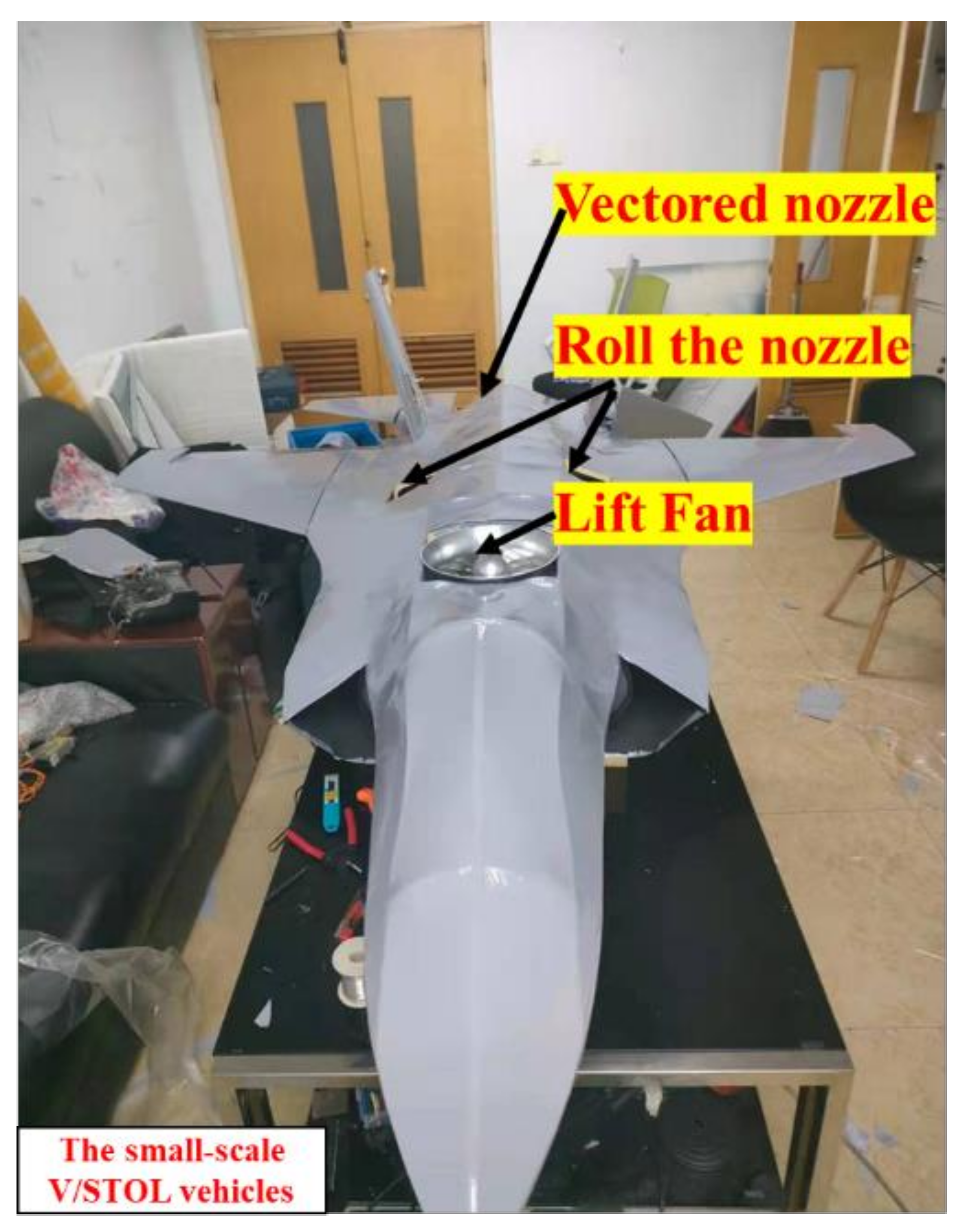
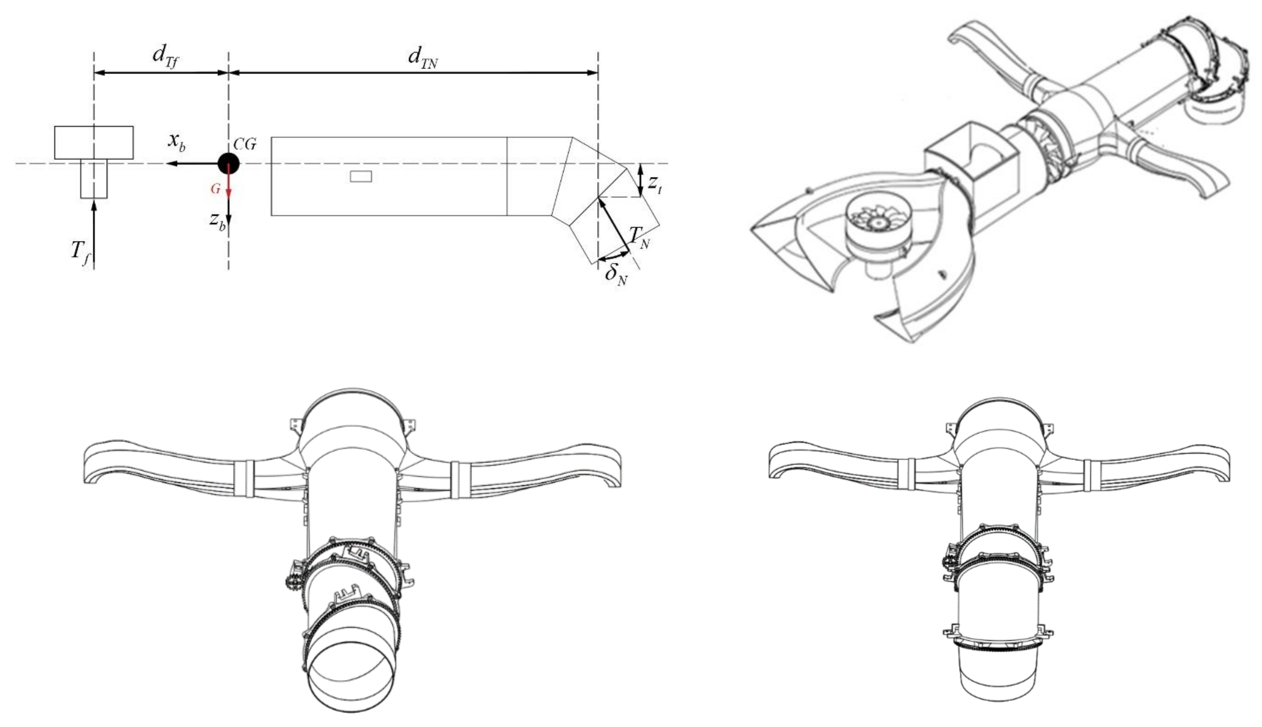
2.1. The Propulsion System Model

The control principle of the thrust-vectored aircraft is illustrated in Figure 2, with the crucial parameters given in

Table 1. General characteristics of power system.

Parameters	Value
$d_{Tf}$	0.476 m
$d_{TN}$	0.561 m
$z_l$	0.1 m

.

For longitudinal control, the vertical thrust component of the 3BSD nozzle $T_N$ and the lift given by the lift-fan $T_f$ work together to balance the gravity and provide pitch control moment. For lateral control, the two side nozzles provide differential thrust, which generates the roll control moment; the roll control and the horizontal thrust components of the 3BSD nozzle generate the yaw control moments for yaw control.

2.2. The Jet Stream Effect

In the transition phase, due to the jet stream effects, the lift generated from the lift-body and 3BSD nozzle is polluted. Thus, the clean aerodynamic lifts and nozzle thrust obtained from wind tunnel tests are not consistent with those in real-world flight, when the lift-fan is on. Empirically, the jet stream effect brings about the lift loss. The lift loss $\frac{\Delta L}{T}$ can be divided into two main parts: the loss of the aerodynamic lifts caused by the low-pressure region that is formed by the jet stream below the wings and the loss of the lift-fan caused by the horizontal inflow blowing away the 3BSD nozzle jet stream. Therefore, the overall lift loss can be expressed by:

$$\frac{\Delta L}{T}=\frac{\Delta L_{\infty }}{T}+\frac{\Delta L_N}{T}$$

(1)

where $\Delta L$ is the overall lift loss, $\Delta L_{\infty }$ is the aerodynamic lift loss caused by lift-fan jet stream, $\Delta L_N$ is the 3BSD nozzle lift loss and $T$ is the lift of the lift-fan. According to the empirical function in [1,5], these two parts can be written as:

$$\frac{\Delta L_{\infty }}{T}=-0.002528\sqrt{\frac{S}{A_j}}{(N_{PR}{}^{-0.64}\frac{P_{er}}{d_{ne}})}^{1.581}$$

(2)

$$\frac{\Delta L_N}{T}=K_A{K}_c(35V_e^{5.5}(\sqrt{\frac{S}{A_j}}-1)-3V_e^2{(\sqrt{\frac{S}{A_j}}-1)}^{\frac{2}{3}}){\delta }_j$$

(3)

where $S$ is the reference area, $A_j$ is the nozzle area, $N_{PR}$ is the nozzle pressure ratio, $P_{er}$ is the perimeter of the nozzle, $d_{ne}$ is the equivalent diameter of the nozzle, $V_e$ is the equivalent velocity ratio defined as $V_e=\sqrt{\frac{Q}{q_j}}$, with $Q$ and $q_j$ indicating the dynamic pressure of the inflow and nozzle jet stream, respectively, ${\delta }_j$ is the deflection angle of the nozzle, $K_A$ is the correction factor of the aspect ratio, and $K_C$ is the correction factor of the nozzle mounting position.

In this work, the nozzles include the lift-fan nozzle, the 3BSD nozzle and the side nozzles. Concerning the fact that the lift-fan is mounted near the main wings but far away from the tails, the jet stream effect of the lift-fan only influences the main wings. The 3BSD nozzle locates near the horizontal tails but is fairly far away from the main wings; thus, its jet effect only impacts the tail wings. The two side nozzles are neglected for they are mounted outside the wings. The inflow effects can be regarded as only influencing the lift-fan jet stream. Therefore, the overall lift loss is constructed as:

$${(\frac{\Delta L}{T})}_{all}={(\frac{\Delta L_{\infty }}{T})}_w+{(\frac{\Delta L_{\infty }}{T})}_t+{(\frac{\Delta L_N}{T})}_f$$

(4)

where ${(\frac{\Delta L}{T})}_{all}$ refers to the total lift loss, ${(\frac{\Delta L_{\infty }}{T})}_w$ is the main wing lift loss caused by lift-fan, ${(\frac{\Delta L_{\infty }}{T})}_t$ is the tail wing lift loss caused by 3BSD nozzle, ${(\frac{\Delta L_t}{T})}_f$ is the lift-fan lift loss caused by the inflow. Their specific value can be determined by Equations (2) and (3).

Besides, the lift loss will cause the pitch moment variation, which can be calculated by Equation (5):

$$\frac{\Delta M}{T{D}_e}=\frac{\Delta L}{T}\frac{X_j}{D_e}$$

(5)

where $D_e$ is the equivalent diameter of the nozzle exits, $\frac{\Delta L}{T}$ is the variation of the moments, $\frac{X_j}{D_e}$ is the acting point of the lost lift. For this work, the lost lift in Equation (4) can be assumed to act on the aerodynamic center of the main wings and tail wings, and the lift-fan mounting point.

To simplify the expression, the lift loss and pitch moment variation are indicated as:

$$\left\{\begin{array}{c}{T}_f^n=T_f-T_f{(\frac{\Delta L}{T})}_{all}=T_f\frac{\partial T_f^n}{\partial T_f}\\ M^n=T_f{d}_{T_f}-\Delta M=T_f\frac{\partial T_f^n}{\partial T_f}{d}_{T_f}^n\end{array}\right.$$

(6)

where $T_f^n$ is the equivalent lift loss on lift-fan, $M^n$ is the equivalent pitch moment variation around lift-fan, $d_{T_f}^n$ is the equivalent arm of force.

The jet-induced effect is calculated by the formulas above and the results in the transition phase are given in Figure 3.

2.3. Longitudinal Dynamic Model

Having constructed the lift loss caused by the jet stream effects, the longitudinal 3 degrees of freedom (3-DOF) dynamic function can be written as:

$$\left\{\begin{array}{l}{\dot{V}}_x=(T_N\cos {\delta }_N+QS{C}_L\sin \alpha -QS{C}_D\cos \alpha -G\sin \theta )/m\hfill \\ {\dot{V}}_z=(-T_N\sin {\delta }_N-QS{C}_L\cos \alpha -QS{C}_D\sin \alpha -T_f\frac{\partial T_f^n}{\partial T_f}+G\cos \theta )/m\hfill \\ \dot{q}=(-T_N\sin {\delta }_N{d}_{T_N}-QS{C}_{m}b-QS{C}_D\sin \alpha -T_f\frac{\partial T_f^n}{\partial T_f}{d}_{T_f}^n)/I_{yy}\hfill \\ \dot{\theta }=q\hfill \end{array}\right.$$

(7)

where ${\dot{V}}_x$ and ${\dot{V}}_z$ are the acceleration along body x-axis and z-axis, respectively, $\dot{q}$ and $\dot{\theta }$ are the pitch angular acceleration and angular rate, respectively, $Q$ is the dynamic pressure, $b$ is the reference span, $C_L$, $C_D$ and $C_m$ are the aerodynamic lift, drag and pitch moment coefficients, respectively, $m$ is the mass, $g$ is the acceleration of gravity, $I_{yy}$ is the rotational inertia of the body y-axis. The 3-DOF function can be reduced to the state-space equation:

$$\dot{x}=f(x,u)$$

(8)

where $x$ is the state variables and $u$ is the control inputs.

The specifications (e.g., mass, moment of inertia, cruise velocity, etc.) of the F-35B prototype are illustrated in

Table 2. Specifications of the prototype F-35B model.

Parameters	Values
$m$	13 kg
$S$	0.88 m2
$b$	1.53 m
$I_{yy}$	1.055 kg/m3

. And the aerodynamic data of the prototype F-35B is acquired by wind tunnel experiments, which provides high-quality data to ensure the fidelity of the simulation. Correspondingly, 3D printing technology is used for the wind tunnel experiments, as shown in Figure 4. Relevant aerodynamic information, including stability and control derivatives, is available at (https://doi.org/10.5281/zenodo.5797173) (accessed on 30 March 2022).

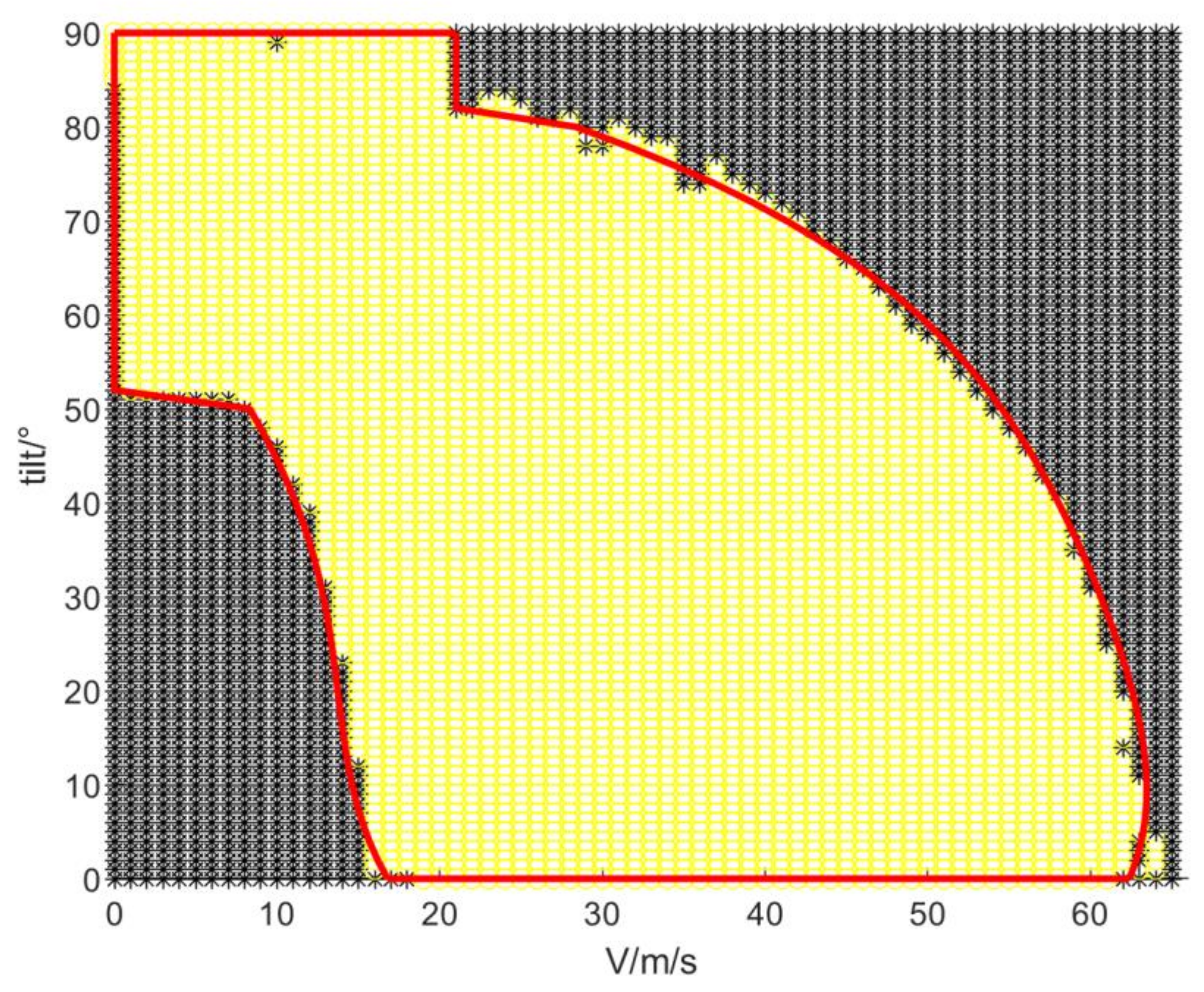
2.4. Transition Corridor

The transition corridor is constructed using AES methods. AES is the equilibrium point set that the aircraft can achieve inside the control efficiency boundaries, which is widely used in the controllable boundary establishment of aircrafts.

The aim of the trimming process is to find the control inputs that make the vehicle self-balanced under certain states. With Equation (8), the longitudinal trimming is to calculate the required $u$ to let $\dot{x}=0$ under the certain constraints on $x$ and $u$. After setting the constraint conditions, the equilibrium boundary can be acquired by trimming the aircraft in all possible states. The calculation procedure is shown below:

• Step 1: Initialize the model parameters, calculation conditions and constraint states.
• Step 2: Trim the model and save the results.
• Step 3: Change the trimming velocity and tilt angle of the 3BSD nozzle and repeat Step 2.
• Step 4: Plot the trimming results.
• Step 5: Remove the trimming points that have excessive flight path angles.

The constraints on state variables are:

$$\left\{\begin{array}{l}\dot{\alpha }=0,\dot{q}=0,q=0\hfill \\ {\alpha }_{\min }<\alpha <{\alpha }_{\max }\hfill \\ V_x=V_{Tas}\cos \alpha ,V_z=V_{Tas}\sin \alpha \hfill \\ \begin{array}{l}{\dot{V}}_x=0,{\dot{V}}_z=0\hfill \\ V_{Tas}=V_0\hfill \\ {\delta }_N={\delta }_0\hfill \end{array}\hfill \end{array}\right.$$

(9)

where $\dot{\alpha }$ and $\dot{q}$ are the derivatives of angle attack and pitch angular rate versus time, ${\alpha }_{\min }$ and ${\alpha }_{\max }$ are the boundaries of angle of attack, $u_b$ and $w_b$ are the velocity components along body x-axis and z-axis, $V_{Tas}$ and ${\delta }_N$ are the true airspeed and 3BSD deflection angles.

Besides, the control input’s saturation parameters should be given according to the control efficiency, as shown in

Table 3. The limit of the actuator F-35B.

Actuators	Max Value
${\delta }_e$	[−35°, 35°]
$T_f$	[0, 80 N]
$T_N$	[0, 80 N]
${\delta }_N$	[0, 90°]

.

According to the aforementioned constraint conditions, the aircraft can be trimmed in all possible states. For those single failure points, they can be replaced by their neighbors. The results whose trimming flight path angles $\gamma$ are over 20 degrees are removed to get a smooth transition trajectory. Figure 5 presents the transition corridor. It is reasonable that the left boundary is limited by the tilt angle of the 3BSD nozzle, as the gravity is balanced mainly by the thrust vectors, and the right boundary is limited by the attainable thrust to balance the aerodynamic drag. Having obtained the transition corridor, a straight line is plotted inside the corridor and is chosen as the initial transition trajectory for optimization.

3. Control Strategy

For the thrust-vectoring V/STOLs, the longitudinal physical inputs are lift-fan throttle, 3BSD nozzle throttle, tilt angle of 3BSD nozzle and the elevator deflection angle. To control these physical inputs requires complex control coordination for the pilots. Therefore, the virtual control inputs should be designed first.

3.1. Control Principles

The thrust-vectoring V/STOLs have three control principles in different flight modes, namely, the hovering mode, the transition mode, and the cruising mode. In hovering mode, the longitudinal motion of the control stick will drive the aircraft along the ground z-axis, the latitudinal motion of the control stick will drive the vehicle along the ground y-axis and the throttle stick will control the ground x-axis velocity. In transition mode and cruising mode, the stick responses are similar. In transition mode, the longitudinal stick input ${\delta }_3$ controls the pitch angular acceleration, lateral stick input controls the roll angular acceleration, throttle stick ${\delta }_1$ controls the body x-axis acceleration and the idler wheel ${\delta }_4$ controls the angular rate of the 3BSD nozzle. In cruising mode, the longitudinal stick input controls the elevator, lateral stick input controls the aileron and throttle stick controls the 3BSD nozzle throttle. The control principles are depicted in

Table 4. Control principles of the prototype F-35B.

Stick	Longitude	The z-axis velocity	Pitch acceleration (${\delta }_3$)	elevator
	Lateral	The y-axis velocity	Roll speed	aileron
The throttle lever		The x-axis velocity	The x-axis acceleration (${\delta }_1$)	3BSD nozzle thrust
Pedal		The z-axis angular rates	Rudder	Rudder
Roller		3BSD nozzle tilt angular rates (${\delta }_4$)

.

The overall takeoff/landing strategy is designed as below: Transit modes function at a fixed angle of climb, based on whose value (90 degrees or not), the process is divided into vertical or short.

For takeoff, the pilot drives the vehicle to the safety height by control stick only, in hovering mode. Then, the control stick is released to the neutral point and the throttle stick is pushed for acceleration. Since the throttle stick controls the velocity along the x-axis while in transition mode, and it controls the acceleration along the x-axis, a breakout gear position should be set for the control strategy switch. When the airspeed enters the transition region, the pilot can push the throttle stick, exceeding the breakout gear position and switching to transition mode. During this phase, the throttle stick controls the x-axis acceleration, control stick controls the pitch angular rate, and the idler wheel on the control stick is used to control the 3BSD nozzle-tilting angular rate. Even though the control objects are different in cruising mode and transition mode, the stick response is similar to the pilot. Therefore, when the 3BSD nozzle is completely deflected, the pilot can enter the highspeed cruise mode smoothly.

For landing, the cruising mode is also directly switched to transition mode. The pilot can use the idler wheel to tilt the 3BSD nozzle and enter cruise mode, while for the switch to hovering mode, the throttle stick should be put inside the breakout gear region to enter the hovering mode, when the 3BSD nozzle has deflected completely and the vehicle has decelerated to the threshold velocity.

3.2. Control Allocation

According to the strategy designed before, the control inputs from the pilot correspond to the state variables ${\dot{V}}_x$, $\dot{q}$, ${\dot{\delta }}_N$ in Equation (7):

$$\left\{\begin{array}{c}{\delta }_1={\dot{V}}_x\\ {\delta }_3=\dot{q}\\ {\delta }_4={\dot{\delta }}_N\end{array}\right.$$

(10)

The state variable ${\dot{V}}_z$ is controlled by the flight path angle, which can be calculated by:

$${\dot{V}}_z=\tan ({\theta }_0+\dot{\theta }-{\gamma }_0)(V_x+{\dot{V}}_x)-V_z$$

(11)

Use ${\delta }_2$ to express ${\dot{V}}_z$ and substitute Equations (7)–(8), the linearized result is:

$$\left[\begin{array}{c}m{\delta }_1\\ m{\delta }_2\\ I_{yy}{\delta }_3\end{array}\right]=A_x+B\left[\begin{array}{c}{T}_N\\ {\delta }_e\\ T_f\end{array}\right]$$

(12)

The control input ${\delta }_4$ corresponds to the 3BSD nozzle-tilting angle directly, thus, dismissed. $A_x$ is the state matrix and $B$ is the control matrix, which are written as:

$$A_x=\left[\begin{array}{c}QS[(C_{D\alpha }\alpha +C_D{}_0)\cos \alpha -(C_L{}_{\alpha }\alpha +C_L{}_0)\sin \alpha ]+G\sin \theta \\ QS[(C_D{}_{\alpha }\alpha +C_D{}_0)\sin \alpha +(C_L{}_{\alpha }\alpha +C_L{}_0)\cos \alpha ]-G\cos \theta \\ -QbS(C_m{}_{\alpha }\alpha +C_m{}_0)\end{array}\right]$$

(13)

$$B=\left[\begin{array}{ccc}\cos {\delta }_N& QS(C_{L{\delta }_e}\sin \alpha -C_{D{\delta }_e}\cos \alpha )& 0\\ -\sin {\delta }_N& QS(-C_{L{\delta }_e}\cos \alpha -C_{D{\delta }_e}\sin \alpha )& -\frac{\partial T_f^n}{\partial T_f}\\ -\sin {\delta }_N{d}_{T_n}& QSb{C}_{m{\delta }_e}& -\frac{\partial T_f^n}{\partial T_f}{d}_{T_f}^n\end{array}\right]$$

(14)

In Equation (14), $B_{23}$ and $B_{33}$ are the same as the control derivatives $\frac{\partial F_z}{\partial T_f}$, $\frac{\partial M_y}{\partial T_f}$ in physical meanings, which can be acquired by interpolation. Calculate the pseudo-inverse of $B$ and the allocation methods are designed:

$$\left[\begin{array}{c}{T}_N\\ {\delta }_e\\ T_f\end{array}\right]={\left(B^{\mathrm{T}}B+\epsilon I\right)}^{-1}\left(\left[\begin{array}{c}m{\delta }_1\\ m{\delta }_2\\ I_{yy}{\delta }_3\end{array}\right]-A_x\right)$$

(15)

3.3. Control Strategy Optimization

The optimization problem can be described as searching a set of the transition trajectories for a best one that satisfies the takeoff/landing mission requirements. Such a problem involves the constraints on state variables and control variables and is similar to the optimal control problems, which are composed of the cost function, input variables, initial values, boundary conditions and trajectory constraints.

• Input variables

The variable to optimize is divided into four classes: the four state variables $\{V_x,V_Z,q,\theta \}$, four physical inputs $\{{\delta }_e,T_f,T_N,{\delta }_N\}$ and three control variables $\{{\delta }_3,{\delta }_1,{\delta }_4\}$, and the time period $\left\{t\right\}$. Firstly, the time derivative of the state variables is the control variables, thus, constraining the control variables implicitly. Then, even though the physical inputs relate to the state variables directly, the strong nonlinearity reduces the optimization efficiency significantly and is, thus, not used for state variable constraints. Therefore, the optimization inputs are chosen as the four state variables $\{V_x,V_Z,q,\theta \}$, four physical inputs $\{{\delta }_e,T_f,T_N,{\delta }_N\}$ and the time period $\left\{t\right\}$. The final optimization inputs are written as $\{V_x,V_Z,q,\theta ,{\delta }_e,T_f,T_N,{\delta }_N,t\}$.

2.

Boundary conditions

The boundary conditions are the boundaries of the four state variables and physical inputs during the whole process, which are usually given by the performance boundaries and mission requirements of the aircraft, written as $x(t_{all})$ and $u(t_{all})$. Besides, to achieve the transition mission target, some of these state variables and inputs should be set as extra initial and terminal conditions. The initial conditions are written as $x(t_0)$ and $u(t_0)$, and terminal ones as $x(t_f)$ and $u(t_f)$. The state variable boundary conditions in this work are expressed as:

$$\left\{\begin{array}{l}{q}_{\min }<q(t_{all})<q_{\max }\hfill \\ q(t_f)=0\hfill \\ \theta (t_0)=0\hfill \\ {\theta }_{\min }<\theta (t_{all})<{\theta }_{\max }\hfill \end{array}\right.$$

(16)

where $q_{\min }$ and $q_{\max }$ are the acceptable pitch angular rate boundaries, ${\theta }_{\min }$ and ${\theta }_{\max }$ are the acceptable pitch angle boundaries. Specifically, the limitations on $V_x$ and $V_z$ are reflected in the trajectory constraints. The physical inputs boundaries are:

$$\left\{\begin{array}{l}\begin{array}{l}{\delta }_e(t_0)=0\hfill \\ {\delta }_e{}_{{}_{\min }}<{\delta }_e(t_{all})<{\delta }_e{}_{{}_{\max }}\hfill \\ 0<T_f(t_{all})<T_f{}_{{}_{\max }}\hfill \end{array}\hfill \\ 0<T_N(t_{all})<T_N{}_{{}_{\max }}\hfill \\ {\delta }_N{}_{{}_{0,\min }}<{\delta }_N(t_0)<{\delta }_N{}_{{}_{0,\max }}\hfill \\ \begin{array}{l}0<{\delta }_N(t_{all})<90°\hfill \\ {\delta }_N{}_{{}_{f,\min }}<{\delta }_N(t_f)<{\delta }_N{}_{{}_{f,\max }}\hfill \end{array}\hfill \end{array}\right.$$

(17)

where ${\delta }_e{}_{{}_{\min }}$ and ${\delta }_e{}_{{}_{\max }}$ are the allowable elevator deflection angle boundaries, $T_N{}_{{}_{\max }}$ and $T_f{}_{{}_{\max }}$ are the maximum thrust of the 3BSD nozzle and lift-fan, respectively. ${\delta }_N{}_{{}_{0,\min }}$ and ${\delta }_N{}_{{}_{0,\max }}$ are the tilting angle authority at the beginning of the transition phase, ${\delta }_N{}_{{}_{f,\min }}$ and ${\delta }_N{}_{{}_{f,\max }}$ are the desired terminal tilting angle boundaries.

3.

Trajectory constraints

Firstly, the flight path angle in transition mode is designed to be a fixed value:

$${\gamma }_{ceq}=\gamma (t_{all})-{\gamma }_0=0$$

(18)

where ${\gamma }_0$ is the default flight path angle.

Targeting a smooth transition flight, the gradient of state variables and physical inputs are constrained by the following inequality:

$$\left\{\begin{array}{c}{c}_{\dot{x}}=(\dot{x}-{\dot{x}}_{\max })(\dot{x}-{\dot{x}}_{\min })<0\\ c_{\ddot{x}}=(\ddot{x}-{\ddot{x}}_{\max })(\ddot{x}-{\ddot{x}}_{\min })<0\\ c_{\dot{u}}=(\dot{u}-{\dot{u}}_{\max })(\dot{u}-{\dot{u}}_{\min })<0\\ c_{\ddot{u}}=(\ddot{u}-{\ddot{u}}_{\max })(\ddot{u}-{\ddot{u}}_{\min })<0\end{array}\right.$$

(19)

where $\dot{x}$ and $\ddot{x}$ are the first order and second order derivatives of the state variables, $\dot{u}$ and $\ddot{u}$ are the first order and second order derivatives of the control inputs. ${\dot{x}}_{\max }$,${\dot{x}}_{\min }$, ${\ddot{x}}_{\max }$, ${\ddot{x}}_{\min }$ are the constraints on state variables, ${\dot{u}}_{\max }$, ${\dot{u}}_{\min }$, ${\ddot{u}}_{\max }$, ${\ddot{u}}_{\min }$ are the constraints on control inputs.

To make sure that the transition process ranges inside the transition corridor, the following conditions are given:

$$\left\{\begin{array}{l}{C}_{V_{Tas}}^1=(V_{Tas}(t_0)-V_{0_{\max }})(V_{Tas}(t_0)-0)<0\hfill \\ C_{V_{Tas}}^2=(V_{Tas}(t_f)-V_{f_{\max }})(V_{Tas}(t_f)-V_{f_{\min }})<0\hfill \\ C_{V_{Tas}}^3=(V_{Tas}(t_{all})-V_{Ta{s}_{\max }})(V_{Tas}(t_{all})-V_{Ta{x}_{\min }})<0\hfill \end{array}\right.$$

(20)

where $V_{0_{\max }}$ is the maximum transition speed, $V_{f_{\max }}$, $V_{f_{\min }}$ are the airspeed boundaries, and $V_{Ta{s}_{\max }}$, $V_{Ta{s}_{\min }}$ are the aforementioned velocity-tilting angle envelope.

4.

Cost function

The cost function is set according to the mission requirements. For the takeoff mission, the requirements are smooth transition or minimum fuel rate. Therefore, the corresponding cost function is given below:

$$\min J_{smooth}=D({\dot{\delta }}_1(t))+D({\dot{\delta }}_3(t))+D({\dot{\delta }}_4(t))$$

(21)

$$\min J_{oil\min }={\displaystyle {\int }_{t_0}^{t_f}{T}_f^2(t)+T_N^2(t)}dt$$

(22)

where $D({\dot{\delta }}_1(t))$ is the square deviation of ${\dot{\delta }}_1(t)$.

For the landing mission, the requirements are smooth transition and shortest landing distance. The smooth transition cost function is identical with that for the takeoff mission. The cost function for shortest landing distance is expressed as:

$$\min J_{dist\min }=dis\left(t_f\right)$$

(23)

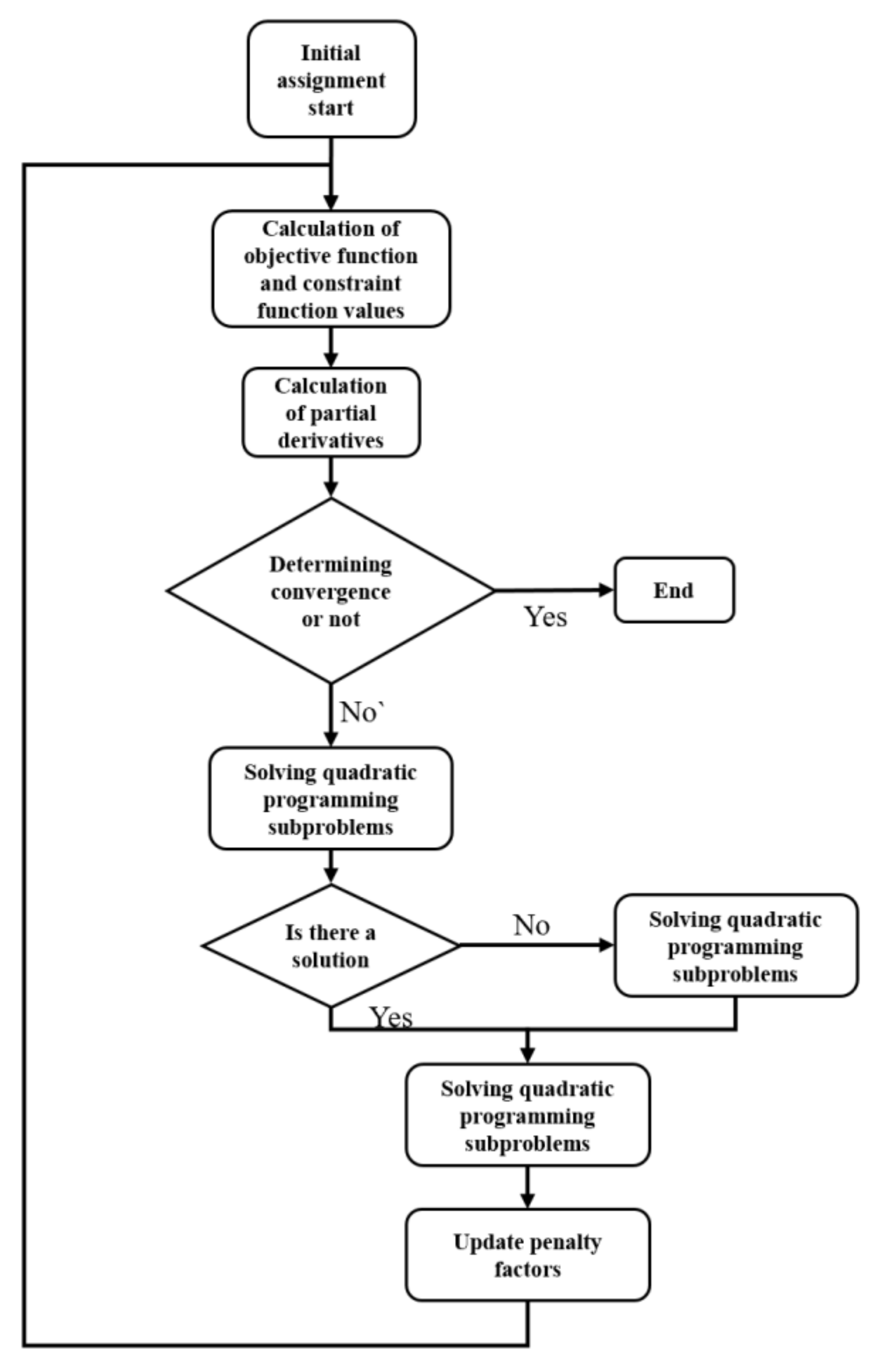
3.4. Numerical Optimization Method

The optimization problem for a thrust-vectoring V/STOL involves considerable variables and complicated parameters, which make it challenging to acquire the analytical solution. Thus, this work applies the direct inverse method to simplify the problem to a nonlinear programing problem, using a sequential quadratic programing (SQR) method to solve it. The flow chart of SQP algorithm is shown in Figure 6.

3.4.1. Nondimensionalization Method

Firstly, the numerical optimization method prefers nearly same-scale variables to calculate, since the variables in higher order of magnitudes would cover the impact of those in lower order. The variables in this work are $\{V_x,V_Z,q,\theta ,{\delta }_e,T_f,T_N,{\delta }_N,t\}$, and the dimensions of these variables determine their order of magnitudes, so the nondimensionalization process is necessary.

The dimensionless variables are defined as $\{{\overline{V}}_x,{\overline{V}}_z,\overline{q},\overline{\theta },{\overline{\delta }}_e,{\overline{T}}_f,{\overline{T}}_N,{\overline{\delta }}_N,t\}$:

$$\left\{\begin{array}{l}{\overline{V}}_x=\frac{k_1{V}_x}{V_{\infty 0}},{\overline{V}}_z=\frac{k_1{V}_z}{V_{\infty 0}}\hfill \\ \overline{q}=\frac{k_{2}qc}{V_{\infty 0}},\hfill \\ \overline{\theta }=k_3\frac{\theta }{{\theta }_{\max }},{\overline{\delta }}_e=k_3\frac{{\delta }_e}{{\delta }_{e\max }},{\overline{\delta }}_N=k_3\frac{{\overline{\delta }}_N}{{\overline{\delta }}_{N\max }}\hfill \\ {\overline{T}}_f=k_4\frac{T_f}{G},{\overline{T}}_N=k_4\frac{T_N}{G}\hfill \end{array}\right.$$

(24)

where $k_1$$k_2$$k_3$$k_4$ are the proportional factors to balance the order of magnitudes of the variables, given as $k_1=k_3=k_4=1$, $k_2=50$, $V_{\infty 0}$ is the standard inflow velocity, which is equal to 10 m/s, $c$ is the reference length, ${\theta }_{\max }$ is the allowed maximum pitch angle, ${\delta }_{e\max }$ and ${\overline{\delta }}_{N\max }$ are the maximum control variables defined in Table 3.

Subjecting Equation (24) to the 3DOF dynamic function (Equation (7)), the control function of the dimensionless variables can be acquired as:

$$\frac{d\overline{x}}{dt}=g(\overline{x},\overline{u})$$

(25)

where $\overline{x}=[{\overline{V}}_x,{\overline{V}}_z,\overline{q},\overline{\theta }]$, $\overline{u}=[{\overline{\delta }}_e,{\overline{T}}_f,{\overline{T}}_N,{\overline{\delta }}_N]$. Further, the optimization conditions can be rewritten in dimensionless format by subjecting Equation (24) to Equations (17)–(23).

3.4.2. Transformation Method

With the nondimensionalized optimization inputs, the direct transformation can be applied to solve the optimization problem.

Firstly, the time period is divided equally to N − 1 parts:

$$\left\{\begin{array}{c}{t}_{all}=t_0~t_f\\ t_0=t_1<t_2\dots <t_k<\dots t_{N-1}<t_N=t_f\\ \Delta t=(t_f-t_0)\\ t_k=t_{k-1}+\Delta t\end{array}\right.$$

(26)

Then, the continuous inputs are discretized as the optimization variables of the nonlinear problem. The discretized inputs are $[{\overline{x}}_1\dots {\overline{x}}_k\dots {\overline{x}}_N,{\overline{u}}_1\dots {\overline{u}}_k\dots {\overline{u}}_N,t_f]$, where N depends on the numbers of sample points, which are selected inside the corridor. The initial values are the trimming state variables and physical inputs of the sample points. The input between the two timestamps are estimated by 3-ordered Hermit interpolation:

$${\overline{x}}_{mk}=\frac{1}{2}({\overline{x}}_k+{\overline{x}}_{k+1})+\frac{\Delta t}{8}[f({\overline{x}}_k,{\overline{u}}_k)-f({\overline{x}}_{k+1},{\overline{u}}_{k+1})]$$

(27)

$${\overline{u}}_{mk}=\frac{1}{2}({\overline{u}}_k+{\overline{u}}_{k+1})$$

(28)

After the discretization of the dynamic function in this work using the Simpson method, the defective equality constraint is:

$${\overline{x}}_{k+1}-{\overline{x}}_k=\frac{\Delta t}{6}(f({\overline{x}}_k,{\overline{u}}_k)+4f({\overline{x}}_{mk},{\overline{u}}_{mk})+f({\overline{x}}_{k+1},{\overline{u}}_{k+1}))$$

(29)

The flight path angle constraint is converted to:

$$0\le {\gamma }_k-{\gamma }_0\le 0$$

(30)

The constraints on state variables and physical inputs are discretized to:

$$\left\{\begin{array}{l}({\dot{\overline{x}}}_k-{\dot{\overline{x}}}_{\max })({\dot{\overline{x}}}_k-{\dot{\overline{x}}}_{\min })<0\hfill \\ ({\ddot{\overline{x}}}_{\mathrm{k}}-{\ddot{\overline{x}}}_{\max })({\ddot{\overline{x}}}_k-{\ddot{\overline{x}}}_{\min })<0\hfill \\ ({\dot{\overline{u}}}_k-{\dot{\overline{u}}}_{\max })({\dot{\overline{u}}}_k-{\dot{\overline{u}}}_{\min })<0 \hfill \\ ({\ddot{\overline{u}}}_k-{\ddot{\overline{u}}}_{\max })({\ddot{\overline{u}}}_k-{\ddot{\overline{u}}}_{\min })<0\hfill \end{array}\right.$$

(31)

At the K-th timestamp, the first order and second order derivatives of the state variables and control inputs are approximately expressed as:

$$\left\{\begin{array}{l}{\dot{\overline{x}}}_k=({\overline{x}}_{k+1}-{\overline{x}}_k)/\Delta t\hfill \\ {\ddot{\overline{x}}}_k=(({\overline{x}}_{k+1}-{\overline{x}}_k)-({\overline{x}}_k-{\overline{x}}_{k-1}))/\Delta t\hfill \\ {\dot{\overline{u}}}_k=({\overline{u}}_{k+1}-{\overline{u}}_k)/\Delta t\hfill \\ {\ddot{\overline{u}}}_k=(({\overline{u}}_{k+1}-{\overline{u}}_k)-({\overline{u}}_k-{\overline{u}}_{k-1}))/\Delta t^2\hfill \end{array}\right.$$

(32)

After the discretization of the trajectory constraints, the constraint numbers correspond to the overall time period and discrete point numbers. The narrow constraint zones will bring about smooth transition trajectories but may cause divergence in Equation (24), while broad constraint zones may cause abrupt change in the results. The parameters used in this work are given in

Table 5. The constraint parameter.

Parameters	Values
$t$	25
${\dot{\overline{x}}}_{\min }$	[−0.5, −0.1, −0.5, −0.5]
${\ddot{\overline{x}}}_{\min }$	[−0.1, −0.1, −0.1, −0.8]
${\dot{\overline{u}}}_{\min }$	[−0.1, −0.1, −0.1, −0.1]
$N$	46
${\dot{\overline{x}}}_{\max }$	[0.5, 0.1, 0.5,0.5]
${\ddot{\overline{x}}}_{\max }$	[0.1, 0.1, 0.1, 0.8]
${\dot{\overline{u}}}_{\max }$	[0.1, 0.1, 0.1, 0.1]

.

The inequality constraints on the initial time and terminal time are discretized as:

$$\left\{\begin{array}{l}({\overline{V}}_{Tas1}-{\overline{V}}_{0_{\max }})({\overline{V}}_{Tas1}-0)<0\hfill \\ ({\overline{V}}_{TasN}-{\overline{V}}_{f_{\max }})({\overline{V}}_{TasN}-{\overline{V}}_{f_{\min }})<0\hfill \\ ({\overline{V}}_{Task}-{\overline{V}}_{Tas{k}_{\max }})({\overline{V}}_{Task}-{\overline{V}}_{Tas{k}_{\min }})<0\hfill \end{array}\right.$$

(33)

where $V_{Tas{k}_{\max }}$ and $V_{Tas{k}_{\min }}$ are the velocity envelope boundaries at corresponding tilting angles.

The discretized cost function of smooth transition is the same as that in nonlinear constraints while that of the minimum fuel rate is discretized to:

$$\min J_{oil\min }={\displaystyle \sum _{k=1}^N[{\overline{T}}_f^2(t_k)+{\overline{T}}_N^2(t_k)}]$$

(34)

For the shortest landing distance, the discretized cost function replaces $dis(t_f)$ with $dis(t_N)$.

4. Optimization Results

The optimization results vary with the flight mission requirements. This work solves the strategy and trajectory optimization problem through the optimal control methods, providing a control strategy reference for pilots.

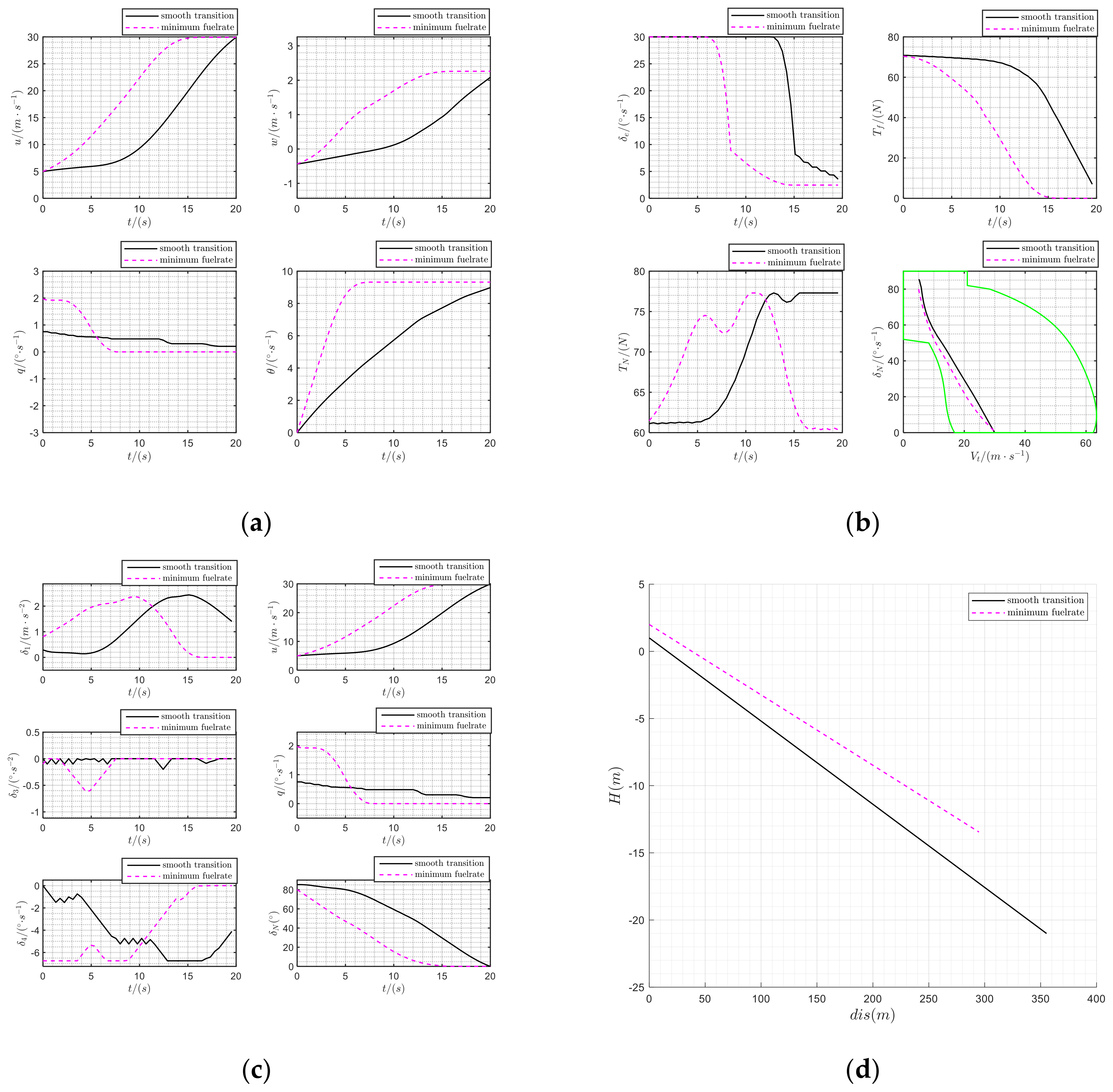
4.1. Transition in Take-Off

The boundary condition and trajectory constraints are given by:

$$\left\{\begin{array}{l}80<{\delta }_N(t_0)<90\hfill \\ 0\le {\delta }_N(t_N)\le 0\hfill \\ (V_{Tas}(t_1)-5)V_{Tas}(t_1)<0\hfill \\ (V_{Tas}(t_N)-30)(V_{Tas}(t_N)-50)<0\hfill \end{array}\right.$$

(35)

The optimization targets are the aforementioned smooth transition and minimum fuel rate. The time histories of the optimization results are given in Figure 7 and Figure 8.

Clearly, with the same constraints, the state variables and control inputs have similar tendencies. For the smooth transition optimization, the control stick variables have obviously smoother curves. Specifically, in the vertical takeoff mission, the control inputs ${\delta }_3$ and ${\delta }_4$ are almost a constant, which lets the pilot complete the transition mission by controlling ${\delta }_1$ only.

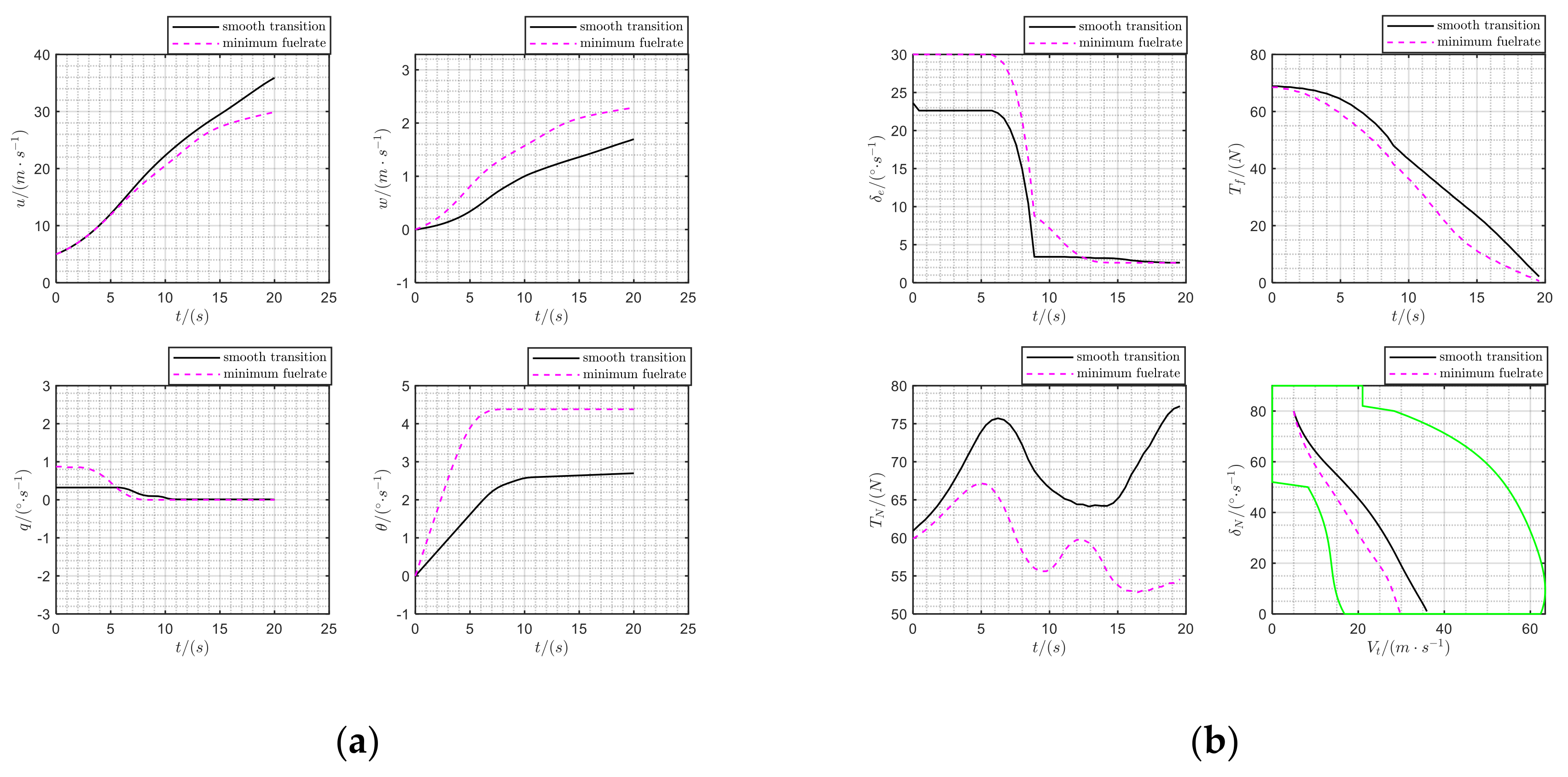
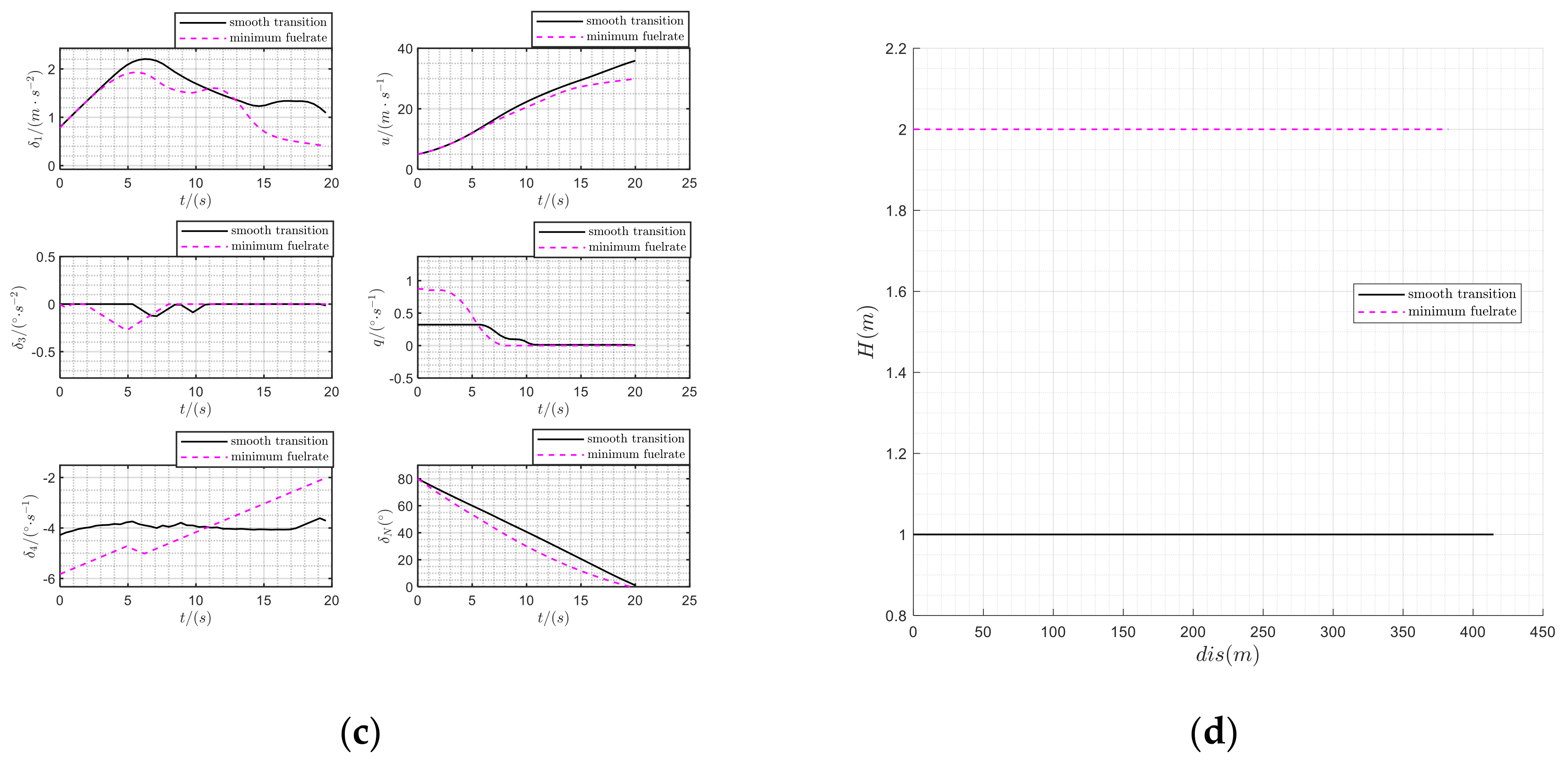
4.2. Transition in Landing

The boundary condition and trajectory constraints for the landing mission are given by:

$$\left\{\begin{array}{l}0\le {\delta }_N(t_0)\le 0\hfill \\ 80<{\delta }_N(t_N)<90\hfill \\ (V_{Tas}(t_1)-30)(V_{Tas}(t_1)-50)<0\hfill \\ (V_{Tas}(t_N)-5)V_{Tas}(t_N)<0\hfill \end{array}\right.$$

(36)

The optimization results are given in Figure 7.

Since the landing is commonly a descending process, the optimization results are given with the negative flight path angle $\gamma$. The time history results are given in Figure 9. For a shorter landing distance, a quicker deceleration is required, resulting in a bigger absolute value of the control input ${\delta }_1$. On the other hand, the aircraft has to pitch up for a larger angle of attack to fly stably. Therefore, the control input ${\delta }_3$ should have a big absolute value too. For a quicker transition process, the tilting rate of the 3BSD nozzle should be large and, thus, the absolute value of the control input ${\delta }_4$ should also be large. From Figure 9c, the optimization results are reasonable in physics.

5. Conclusions

This work conducted a systematic study on the transition process for thrust-vectoring V/STOL aircrafts. Firstly, the dynamic model of the propulsion system is established by the empirical function of the jet stream. Then, the transition corridor is established by the AES methods. To address the problems in redundant physical inputs, the control principles in the transition phase are designed and the allocation criteria are given. Finally, the optimal control strategies are solved based on optimal control theory. The following conclusions can be verified:

Firstly, the corridor establishment based on the AES method is successful, since the results presented in Figure 5 reflect the physical characteristics of the study object and provide a specific reference for the optimization process. The building logic is simple and model based, which released us from the complicated piecewise performance analysis; thus, the corridor with the flight dynamics model can be constructed.

Secondly, the control strategy given in Table 2 is pilot friendly, which ensures a smooth transition between different flight modes, because the strategy considers the control of the sticks and pedals instead of the physical actuators.

Finally, the optimization method is flexible for each flight mission; namely, vertical takeoff/landing to forward flight, short takeoff to forward flight, forward flight to short takeoff/landing and forward flight to hovering. The results reflect the optimization objectives perfectly, as shown in Figure 7, Figure 8 and Figure 9, where the optimized curves vary significantly, though the results achieve the goal of the smooth transition or high transition efficiency.

Overall, the control optimization of the F35B reduced-scale protype successfully addresses the transition control of the tilt angle of the 3BSD nozzles and achieves the target of a safe and efficient transition flight. Work currently being carried out is paying attention to the realization of the proposed optimal control strategy in real flight. In addition, the short takeoff and landing control strategy on the moving platform, such as on a ship, is also studied.

References

1. Jet-Induced Effects. The Aerodynamics of Jet-and Fan-Powered V/STOL Aircraft in Hover and Transition. Available online: http://library.oum.edu.my/oumlib/node/720068 (accessed on 11 April 2022).
2. Franklin, J.A. Revised Simulation Model of the Control System, Displays, and Propulsion System for an ASTOVL Lift Fan Aircraft; NASA-TM-112208; NASA: Washington, DC, USA, 1997; pp. 1–70.
3. Bordignon, K.; Bessolo, J. Control allocation for the X-35B. In Proceedings of the 2002 Biennial International Powered Lift Conference and Exhibit, Williamsburg, VA, USA, 5–7 November 2002. [Google Scholar]
4. Hwang, S.J.; Kim, Y.S.; Lee, M.K. Tilt rotor-wing concept for multi-purpose VTOL UAV. Int. J. Aeronaut. Space Sci. 2007, 8, 87–94. [Google Scholar] [CrossRef] [Green Version]
5. Choi, S.; Kang, Y.; Chang, S.; Koo, S.; Kim, J.M. Development and conversion flight test of a small tiltrotor unmanned aerial vehicle. J. Aircr. 2010, 47, 730–735. [Google Scholar] [CrossRef]
6. Fan, Y.; Wang, X.; Hu, Z.; Zhang, K. Nonlinear modeling and transition corridor calculation of a tiltrotor without cyclic pitch. In MATEC Web of Conferences, Proceedings of the ICPCM2021, Xiamen, China, 29–30 December 2021; EDP Sciences: Les Ulis, France, 2022. [Google Scholar]
7. Tol, H.J.; de Visser, C.C.; van Kampen, E.-J.; Chu, Q.P. Nonlinear Multivariate Spline-Based Control Allocation for High-Performance Aircraft. J. Guid. Control Dyn. 2014, 37, 1840–1862. [Google Scholar] [CrossRef] [Green Version]
8. Tian, Y.; He, Y.; Li, X.; Zhu, J. Simulation testing method of V/STOL flight control strategy. In Proceedings of the 10th World Congress on Intelligent Control and Automation, Beijing, China, 6–8 July 2012. [Google Scholar]
9. Denham, J.; Paines, J. Converging on a Precision Hover Control Strategy for the F-35B STOVL Aircraft. In AIAA Guidance, Proceedings of the Navigation & Control Conference & Exhibit, Honolulu, HI, USA, 18–21 August 2008; American Institute of Aeronautics and Astronautics: Reston, VA, USA, 2008. [Google Scholar]
10. Betts, J.T. Survey of Numerical Methods for Trajectory Optimization. J. Guid. Control. Dyn. 1998, 21, 193–207. [Google Scholar] [CrossRef]
11. Jorris, T.R.; Cobb, R.G. Three-Dimensional Trajectory Optimization Satisfying Waypoint and No-Fly Zone Constraints. J. Guid. Control Dyn. 2008, 31, 543–553. [Google Scholar] [CrossRef]
12. Lee, S.; Bang, H. Three-Dimensional Ascent Trajectory Optimization for Stratospheric Airship Platforms in the Jet Stream. J. Guid. Control Dyn. 2007, 30, 1341–1351. [Google Scholar] [CrossRef]
13. Dragan, A.D.; Ratliff, N.D.; Srinivasa, S.S. Manipulation planning with goal sets using constrained trajectory optimization. In Proceedings of the IEEE International Conference on Robotics & Automation, Shanghai China, 15 August 2011. [Google Scholar]
14. Hughes, S.P.; Mailhe, L.M.; Guzman, J.J. A Comparison of Trajectory Optimization Methods for the Impulsive Minimum Fuel Rendezvous Problem. In Proceedings of the 26th Annual Guidance and Control Conference, Breckenridge, CO, USA, 5–9 February 2003. [Google Scholar]
15. Miele, A.; Wang, T.; Basapur, V. Primal and dual formulations of sequential gradient-restoration algorithms for trajectory optimization problems. Acta Astronaut. 1986, 13, 491–505. [Google Scholar] [CrossRef]
16. Rysdyk, R.T.; Calise, A.J. Adaptive model inversion flight control for tilt—Rotor aircraft. J. Guid. Control Dyn. 1999, 22, 402–407. [Google Scholar] [CrossRef] [Green Version]
17. Brick, S.; Fischer, D. CV-22 osprey flight path cueing flight director system. In Proceedings of the AHS Annual Forum Proceedings, Washington, DC, USA, 20–22 May 1998; AHS International: Fairfax, VA, USA, 1998. [Google Scholar]
18. Klein, P.D.; Nicks, C.O. Flight director and approach profile development for civil tihrotor terminal area operations. In Proceedings of the AHS 54th International Annual Forum, Washington, DC, USA, 20–22 May 1998; AHS International: Fairfax, VA, USA, 1998. [Google Scholar]
19. Calise, A.J.; Rysdyk, R. Research in Nonlinear Flight Control for Tihrotor Aircraft Operating in the Terminal Area; NASA CR-203112; NASA: Washington, DC, USA, 1996.
20. Marr, R.L.; Roderick, W.E.B. Handling qualities evaluation of the XV-1 5 tilt rotor aircraft. J. Am. Helicopter Soc. 1975, 20, 23–33. [Google Scholar] [CrossRef]
21. Pu, H.Z.; Zhen, Z.Y.; Gao, C. Tiltrotor aircraft attitude control in conversion mode based on optimal preview control Guidance. In Proceedings of the Navigation and Control Conference, Yantai, China, 8–10 August 2014. [Google Scholar]
22. Bottasso, C.L.; Croce, A.; Leonello, D.; Riviello, L. Optimization of critical trajectories for rotorcraft vehicles. J. Am. Helicopter Soc. 2005, 50, 165–177. [Google Scholar] [CrossRef]
23. Jhemi, A.A.; Carlson, E.B.; Zhao, Y.J.; Chen, R.T. Optimization of rotorcraft flight following engine failure. J. Am. Helicopter Soc. 2004, 49, 117–126. [Google Scholar]
24. Carlson, E.B.; Zhao, Y.J. Optimal city-center takeoff operation of tiltrotor aircraft in one engine failure. J. Aerosp. Eng. 2004, 17, 26–39. [Google Scholar]
25. Birckelbaw, L.G.; Mcneil, W.E.; Wardwell, D.A. Aerodynamics model for a generic ASTOVL lift-fan aircraft. NASA Tech. Rep. 1995, 124, 109–125. [Google Scholar]
26. Smith, B.E.; Pppen, W.A.; Lye, J.D. Propulsion-induced aerodynamic effects measured with a full-scale stovl model. J. Aircr. 2015, 31, 306–313. [Google Scholar] [CrossRef]
27. Thondiyath, A. Design, analysis, and testing of a hybrid vtol tilt-rotor uav for increased endurance. Sensors 2021, 21, 5987. [Google Scholar]
28. Saddington, A.J.; Knowles, K. A review of out-of-ground-effect propulsion-induced interference on stovl aircraft. Prog. Aerosp. Sci. 2005, 41, 175–191. [Google Scholar] [CrossRef]
Figure 1. F-35B reduced ratio aircraft model.
Drones 06 00129 g001
Figure 2. Longitudinal control principle of power system.
Drones 06 00129 g002
Figure 3. Lift loss in transition phase.
Drones 06 00129 g003
Figure 4. The wind tunnel experiment relying on 3D printing technology.
Drones 06 00129 g004
Figure 5. Conversion corridor of V/STOL aircraft.
Drones 06 00129 g005
Figure 6. Flow chart of SQP algorithm.
Drones 06 00129 g006
Figure 7. Optimal solution for tilting transition process of short takeoff; (a) state change curve during short takeoff transition; (b) change curve of physical input during short takeoff transition; (c) control variable variation curve during short takeoff transition; (d) Trajectory change curve of short takeoff transition process.
Drones 06 00129 g007
Figure 8. Optimal solution for tilting transition process of vertical takeoff; (a) state change curve of vertical takeoff transition process; (b) physical input variation curve during vertical takeoff transition; (c) control variable variation curve during vertical takeoff transition; (d) trajectory change curve of vertical takeoff transition process.
Drones 06 00129 g008aDrones 06 00129 g008b
Figure 9. Optimal solution for tilting transition process of short landing; (a) state change curve during short landing transition; (b) change curve of physical input during short landing transition; (c) control variable variation curve during short landing transition; (d) short landing transition trajectory changes curve.
Drones 06 00129 g009