Abstract
In this study, experimental investigations are used to explore the wake propagation and characteristics of a multi-rotor unmanned air vehicle (UAV) in a forward flight mission. Qualitative smoke visualization is used first to gain a qualitative understanding of wake characteristics above and below the body of the multi-rotor UAV which is used as guidance for quantitative particle image velocimetry (PIV) experiments which better resolve the region in the vicinity of the multi-rotor UAV body. The experimental results over a wide range of advance ratios show that as the advance ratio increases, achieved by either lower rotor speeds or higher flight speeds, the distance by which the wake propagates below the UAV is reduced. While above the UAV, the flow returns to the freestream flow closer to the body as the advance ratio increases. Therefore, this study concludes that proximity effects are reduced as the advance ratio increases. Findings from this study can be used to inform in situ sensor placement so that sensor readings are minimally affected by the wake from the multi-rotor UAV. Velocity measurement corrections are provided for sensors mounted above the UAV which can be used to improve sensor data reliability in forward flight. These results can advance autonomous sensing and increase the utility of multi-rotor UAV observations while providing designers and users further guidance to avoid proximity effects.
1. Introduction
Unmanned aerial vehicles (UAVs) are commonly used for a wide variety of applications in many different industries. There has been significant research focused on the design, optimization, and application of UAVs that has greatly increased their utility due to improvements in their performance. There are many different types of UAVs, each with their own advantages and disadvantages. However, fixed-wing and multi-rotors are currently the most popular for industrial applications and for hobbyists alike due to their accessibility, ease of use, and efficacy [1,2]. Although fixed-wing systems can complete long-range missions due to their endurance, they lack maneuverability including the ability to perform hovering and vertical flights. In addition, fixed-wing systems typically require runways for takeoff and landing which are often not available in complex terrain [3]. Multi-rotor systems offer a unique solution to the shortcomings of fixed wing aircrafts as they possess the ability to perform hovering flight and vertical flight (ascending and descending) with ease and can take off with no runway. These capabilities make the multi-rotor platform the ideal candidate for many applications that require high maneuverability and hovering or vertical flight.
Multi-rotors are commonly used for surveillance, imaging, bridge inspections, and other applications near obstacles where their maneuverability and unique flight characteristics can be taken advantage of [4,5,6,7,8,9,10]. In addition, multi-rotors have the potential to be outfitted with in-situ sensors and used for sensing applications, such as emission monitoring, temperature measurements, and atmospheric sampling [11,12,13,14,15]. Multi-rotors are also popular choices for swarm or formation flight—an increasingly popular area of research—due to their high maneuverability [15].
Many of the applications discussed above require an understanding of the wake of the unmanned vehicle as the wake can have an adverse effect on the vehicle. Examples of this phenomenon include operation near obstacles, performance or reliability of sensor data from the on-board instrumentation, and wake interaction between rotors onboard the drone or from nearby drones. Multi-rotors or other rotary-wing systems commonly exhibit proximity effects when operating near obstacles to include ground-effect, ceiling-effect, or effects from neighboring vehicles in swarm flight. When rotary-wing vehicles operate near the ground, ground effects can be observed which increase the thrust from the vehicle due to the wake interaction with the ground [16]. This phenomenon has been thoroughly studied for helicopters, but is not understood as well for multi-rotors [17,18]. Similarly, ceiling-effect occurs when a rotary-wing is operated near a ceiling obstacle and can cause an increase in thrust production which can be detrimental as it can cause the vehicle to be pulled into the ceiling [19]. Since these proximity effects can have such a negative result and cause catastrophic failure, it is imperative that wake propagation is understood and can be accurately predicted to avoid failure. Aside from mission failure, the wake from these vehicles can contaminate observations from integrated in-situ instrumentation used for autonomy, emission monitoring, and atmospheric sampling that relies upon access to freestream flow which can be affected from the wake of the vehicle [20]. In order to obtain reliable sensor data, all instrumentation should be properly placed on the vehicle, outside the wake region. The wake can also affect the transportation of particulates—such as pollution, dust, or insecticides and herbicides—in the atmosphere [21]. To locate sensors in regions of minimal disturbance, it is imperative to characterize the wake to determine if such regions exist, where they are, and under what flight conditions.
Although proximity effects do not necessarily give a full description of the wake from a rotary-wing vehicle, they provide insight into the wake patterns and strength as the wake propagates from the vehicle. Proximity effects have been studied in similar structures such as helicopters, using an experimental approach and comparing the obtained data to models [22]. From these studies, the proximity effect models that have been accepted for helicopters show discrepancies in comparison to the experimental data from multi-rotors, thus making them unreliable for our applications. Some studies have applied correction factors to fix these discrepancies so that the ground effect can be accurately predicted [23]. In addition, some researchers have used similar correction techniques to predict ceiling effects [24]. There are some studies using computational fluid dynamics (CFD) studies to analyze the ground effect for multi-rotors, confirming that there is a decrease in drag and increase in lift in close proximity to the ground [25,26].
Other researchers have focused more deeply on performance, wake characteristics, and propagation from both multi-rotor and single-rotor systems. These studies have been carried out using computational fluid dynamics (CFD) or experimental studies to include particle image velocimetry (PIV) [26,27,28,29,30,31,32,33,34,35,36,37,38,39,40]. Some of these studies have demonstrated how the Reynolds number affects wake propagation, but they do not provide results with respect to the advance ratio which is a highly influential parameter [32,33]. Zhou et al. [34] have conducted one of the most in-depth investigations of wake behavior with respect to advance ratio, but they focused on the effect to the drone itself. The studied effects relate to propulsive efficiency and thrust coefficient, not disturbance distances or angles due to a limited PIV field of view. Defining disturbance distances and angles is crucial for sensor placement and multi-rotor UAV operation near obstacles.
Previous wake characteristic studies, both CFD and experimental, have provided insight into wake characteristics and structure from multi-rotor UAVs; however, additional studies are needed to characterize the wake propagation distance due to vehicle parameters and flight conditions to prevent catastrophic failure when in close proximity to obstacles and to ensure reliable in situ sensor data. For more information on the mentioned studies in addition to more regarding multi-rotor and single-rotor wake characterization, the reader is referred to [40].
In this work, an experimental approach is taken to study wake propagation from multi-rotors in a forward flight configuration. Flow visualization using illuminated smoke and PIV are employed to study wake characteristics in a wind tunnel over a wide range of flight parameters. Flow visualization results are used to influence and inspire PIV testing. From results gathered from PIV testing, non-dimensional parameters based on vehicle geometry and flow characteristics are developed for the wake prediction and to correct velocity sensor measurements above the multi-rotor UAV. This work is the most in-depth experimental investigation of multi-rotor UAV wake characteristics in forward flight under various flight conditions. These results can be used by users and designers to determine appropriate in-situ instrumentation placement for atmospheric sampling and particulate modeling, as well as in applications such as applying insecticide and herbicide. The remainder of this study is organized as follows: In Section 2, experimental setups used for flow visualization and PIV experiments are described and discussed. The results of visualization and the PIV experiments are presented and discussed in Section 3. Lastly, conclusions and summaries are given in Section 4.
2. Experimental Setup and Measurements
Flow visualization and PIV experiments were conducted in the NMSU low-speed wind tunnel, shown in Figure 1a, which has cross-sectional dimensions of 1.2 × 1.2 m. For the flow visualization experiments, an Aerolab smoke generator is used to feed smoke into the wind tunnel through copper tubing with small holes to generate smoke streaks. To illuminate the streaks, a 532 nm, 200 mW continuous wave laser is placed beneath the wind tunnel that is equipped with a 60-degree Powell lens to generate a laser sheet. A schematic of the flow visualization and PIV setup is provided in Figure 1b where the multi-rotor UAV is mounted to simulate forward flight with an arrow indicating U∞, the freestream flow direction. Although flow visualization techniques are necessary to observe the perturbation of the flow due to the multi-rotor, it is not possible to observe the flow near the body in detail without PIV experiments which occurs over a much smaller field of view (FOV). The PIV system is composed of a dual-cavity Nd-YAG laser (15 pulses/s, 200 mJ/pulse), a high-sensitivity CCD camera (1.4 M pixel, 12-bit gray level), a synchronizer, and a computer to acquire and process images using DaVis 8 software (La-Vision, Inc., Göttingen Germany).
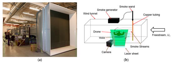
Figure 1.
(a) NMSU wind tunnel and (b) schematic of flow visualization and PIV experimental setup.
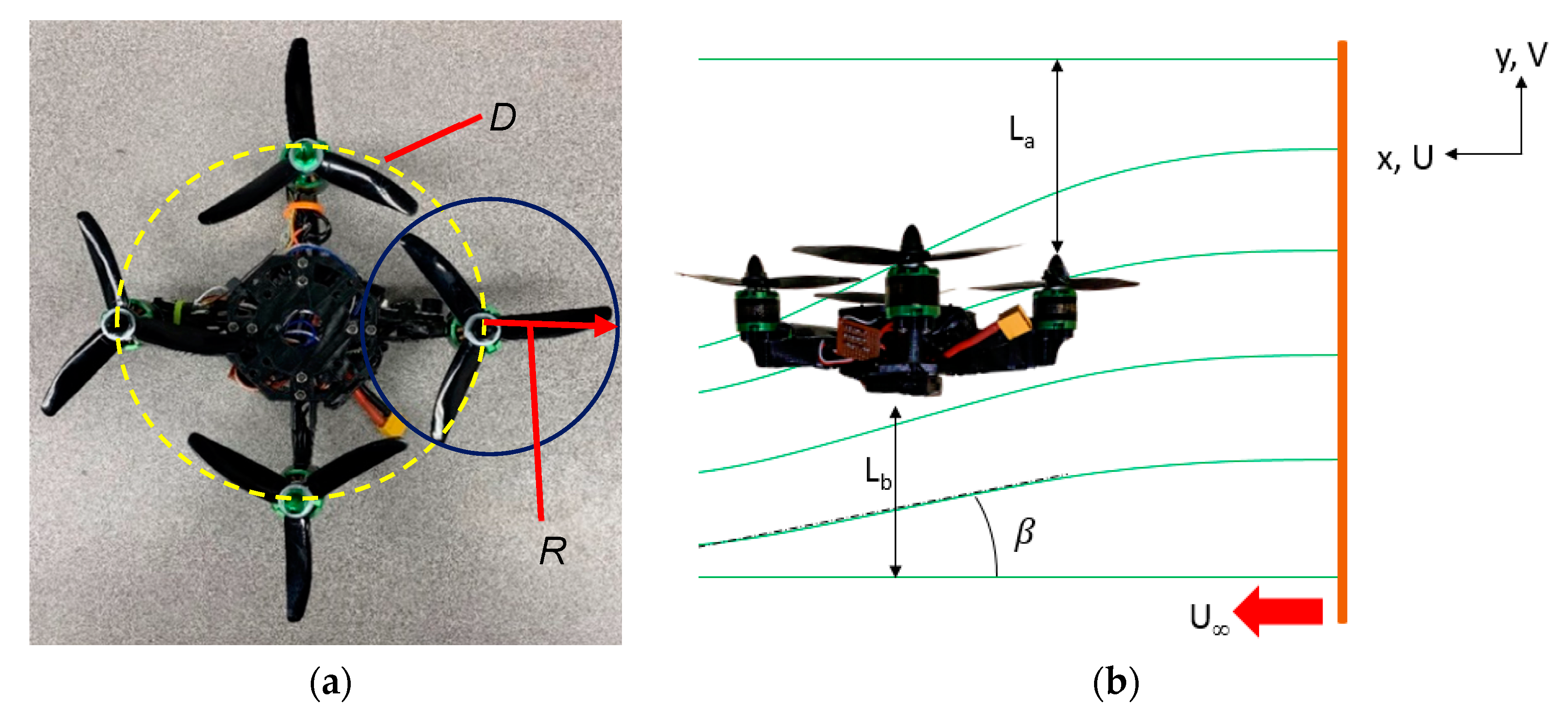
The multi-rotor UAV used for this study is a small UAV with four rotors, each equipped with a three-blade propeller, and it is shown in Figure 2a. The multi-rotor UAV is characterized by a value of 3 where denotes the diameter of the multi-rotor UAV and represents the radius of the propeller, as indicated in Figure 2a. To simulate forward flight, the multi-rotor UAV is mounted to an aluminum rod going through the center of the test section, using a 3D printed mount that allows the UAV to sit horizontally in the wind tunnel to simulate forward flight at a velocity of .
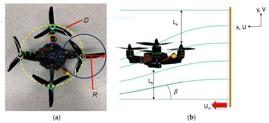
Figure 2.
(a) The multi-rotor UAV used for all experiments including , the diameter of the multi-rotor UAV and , the radius of the propeller. (b) Multi-rotor UAV in simulated forward flight including the disturbance distance both below, and above, the multi-rotor UAV and the angle at which the flow is expelled from the front rotors, β.
In the typical operation of a multi-rotor UAV in forward flight, there is a pitching angle; however, to ensure consistent experimental results under various motor loads, no pitching angle is considered in this study. Preliminary studies considering pitch angles show that the wake from the multi-rotor UAV is rotated and therefore propagates more downstream rather than below it. Considering this, a multi-rotor UAV with no pitch angle represents the upper bound on the distance the wake disturbance propagates before it dissipates into the background flow, referred to as the ‘disturbance distance’ throughout this study. The disturbance distances both below, , and above, , the UAV vary and are therefore discussed separately. In addition, the angle at which the flow is expelled from the front rotors is referred to as the jet angle and is denoted by β. , , and β are shown in Figure 2b, including the coordinate system used throughout the study. Based on the flight conditions, the multi-rotor UAV can be moved vertically to minimize any wall effects caused by the wake interacting with the bottom surface of the tunnel. For experiments focused below the multi-rotor, it is mounted towards the top of the wind tunnel to provide the largest FOV of the wake possible. To investigate the disturbance above the vehicle, the multi-rotor UAV is mounted upside down in the wind tunnel to ensure the FOV is properly illuminated.
3. Wake Propagation Results and Discussions
3.1. Flow Visualization Results
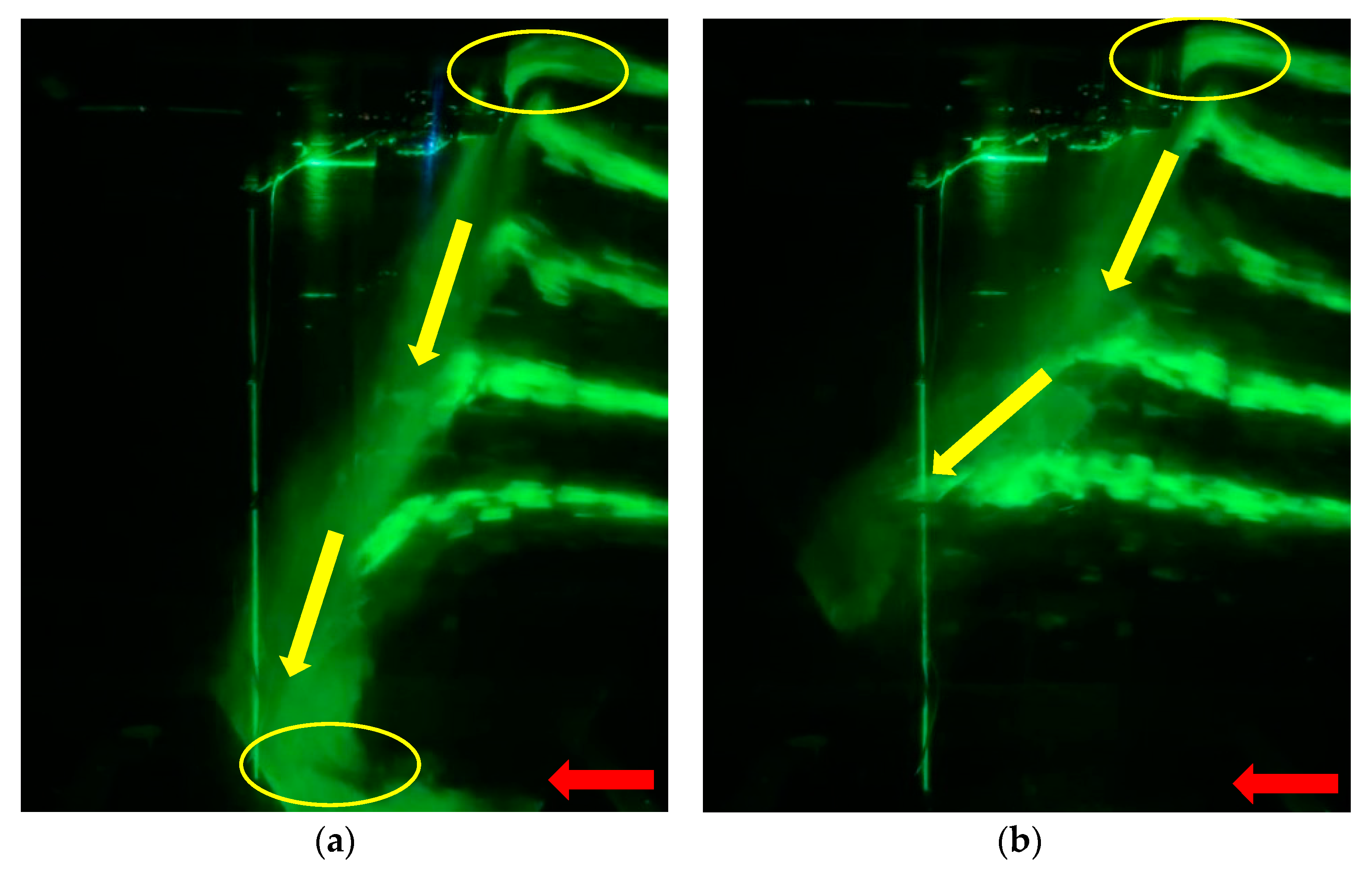
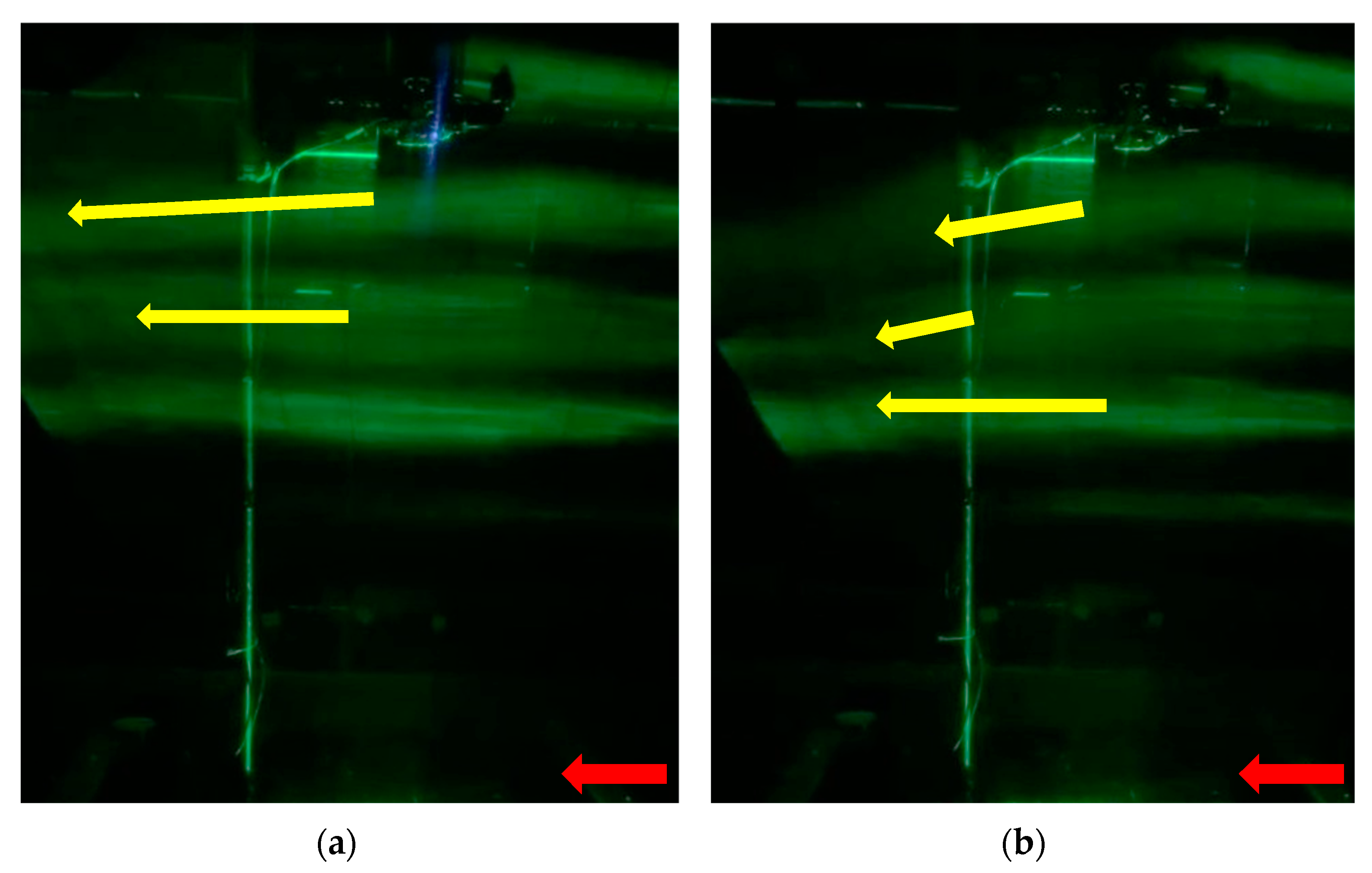
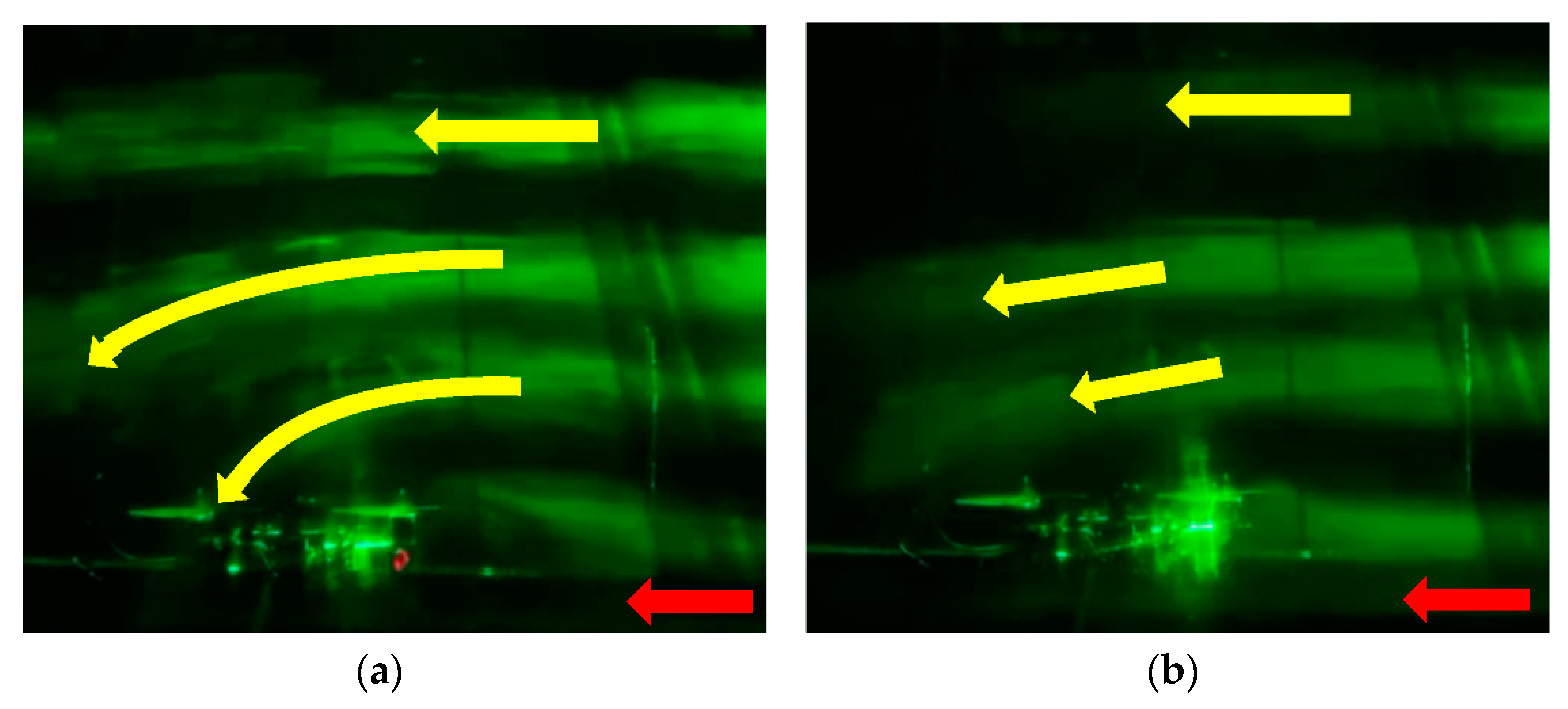
To study the full range of potential flight conditions, experiments are run for —varying from 1 m/s to 5 m/s in 1 m/s increments—and the Reynolds number based on the propeller tip (, where denotes the angular velocity of the rotors (rad/s), represents the rotor radius, is the rotor chord, and is the kinematic viscosity of air) is varied from 3 × 10⁴ to 8 × 10⁴ in increments of 104. In the case of forward flight, the advance ratio is also commonly used to delineate the flow regimes as it considers the forward flight speed and rotor speed simultaneously where the advance ratio is , where is the rotations per second of the propeller. The advance ratios that correspond to the experimental flight conditions are 0.04 0.54. For the results shown in Figure 3 and Figure 4, the red arrow indicates the direction of while yellow arrows highlight and draw attention to significant flow features.

Figure 3.
Flow visualization below the multi-rotor UAV in forward flight at = 1 m/s operating at (a) Retip = 8 × 10⁴ ( = 0.04) and (b) Retip = 5 × 10⁴ ( = 0.06).
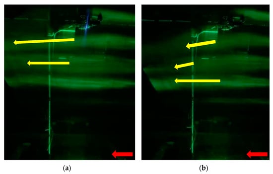
Figure 4.
Flow visualization results from below the multi-rotor UAV in forward flight at = 5 m/s operating at (a) Retip = 3 × 10⁴ ( = 0.54) and (b) Retip = 8 × 10⁴ ( = 0.20).
Considering low and moderate to high Retip values (low advance ratios), it can be seen in Figure 3 that the rotor wake dominates the flow, resulting in large disturbances below the multi-rotor UAV. Figure 3a shows the wake below the multi-rotor UAV with = 1 m/s and Retip = 8 × 10⁴ ( = 0.04) which is the combination of the lowest simulated flight speed and highest rotor speed. This low and high Retip results in strong jets being expelled from the front rotors, beneath the multi-rotor, which extend to the tunnel wall, initiating wall effects that indicate this configuration is beyond the limit of the experimental configuration. As the rotor speed is reduced to Retip = 5 × 10⁴, ( = 0.06), as shown in Figure 3b, there is still a noticeable jet from the rotors, but decreased considerably and is well above the tunnel wall. Furthermore, the angle that the wake propagates from the front rotor is noticeably greater for the = 0.04 condition. As the advance ratio increases to = 0.06, decreases and decreases. In each of the cases, the streamlines are deflected as they are pulled into the rotors and there is a disturbance that extends slightly above the UAV. The disturbance looks minimal, especially in comparison to , but warrants its own investigation in which the FOV of the experiments is focused on the top of the multi-rotor UAV.
For flight conditions characterized by high flight speed, presented in Figure 4, the influence of the rotors is much less discernable than in the previous figure where low freestream speed was considered. Figure 4a,b present the wake from the multi-rotor UAV operating when = 5 m/s and Retip = 3 × 10⁴ ( = 0.54) and Retip = 8 × 10⁴ ( = 0.20), respectively. In both cases, the bottom streamline remains minimally disturbed and continues parallel to the background flow. Although the advance ratio is significantly decreased, there is not a large discrepancy in the wake characteristics in Figure 4b compared to Figure 4a. The increase in rotor speed slightly increases of the wake expelled from the rotors and minimally affects . Aside from these differences, the wake in the two cases is similar.
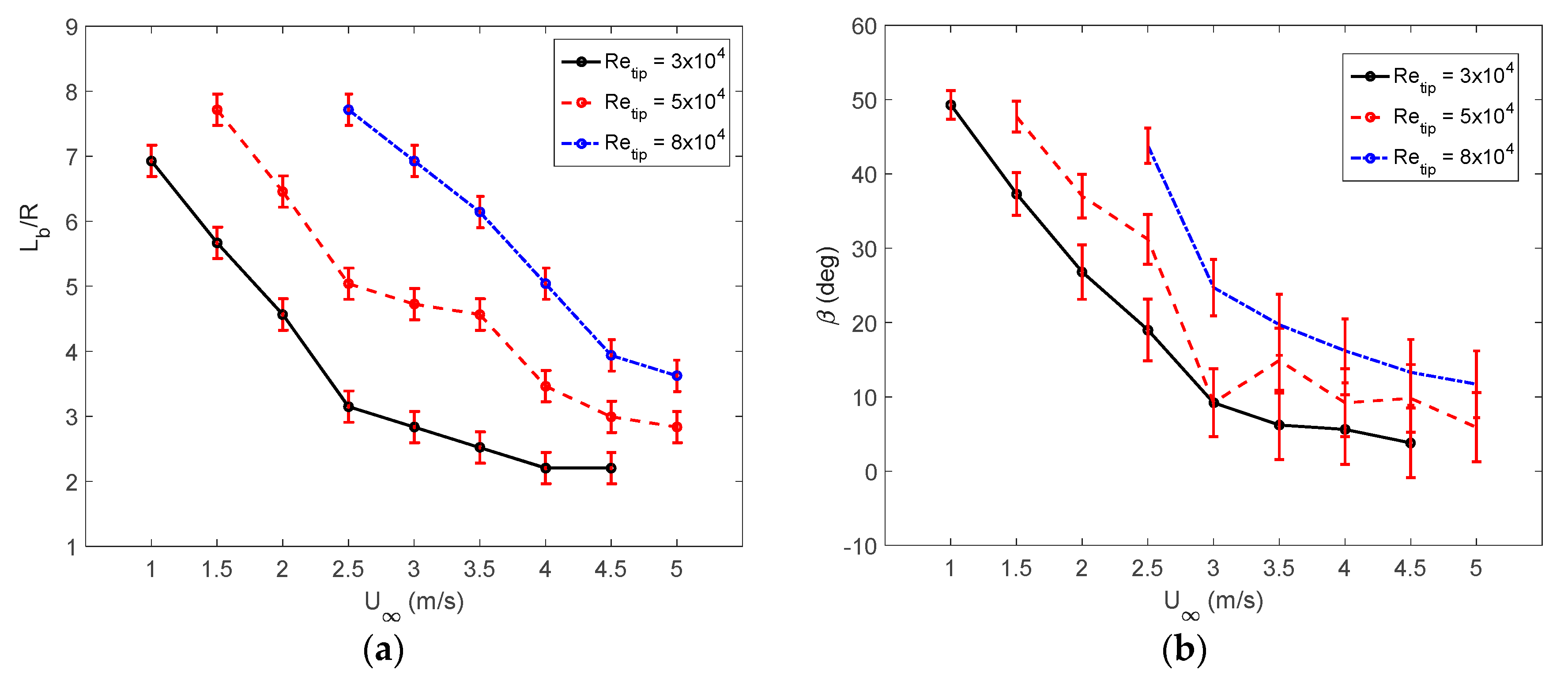
As previously discussed, and from what can be seen in Figure 3 and Figure 4, changes in and rotor speed, Retip, have a clear impact on both and . Figure 5 shows how and are affected as is varied for selected values of Retip. Error bars are provided in both figures based on an estimated 10-pixels of uncertainty () in the vertical measurements for the determination of and , and 2-pixels of uncertainty in horizontal measurements as they are easier to obtain. For these uncertainties, a measurement of was used to determine that for a 12 MP camera, each pixel equals 1.53 mm. Similar trends are observed for both and as is simply the angle between and , the diameter of the multi-rotor UAV. As the Retip is increased—in other words, as the rotor speed increases—for a constant there is an increase in and . There is much greater sensitivity to in the measurement of due to the 10-pixel uncertainty for lower as increases. As is increased, the disturbance distance is reduced, and the wake is expelled from the front rotors at a shallower angle. and are omitted for Retip values when is extended beyond the illuminated FOV or clearly interacted with the tunnel wall.
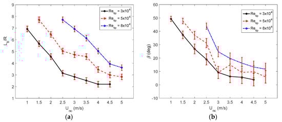
Figure 5.
(a) Disturbance distance, ; and (b) jet angle, for select Retip as a function of .
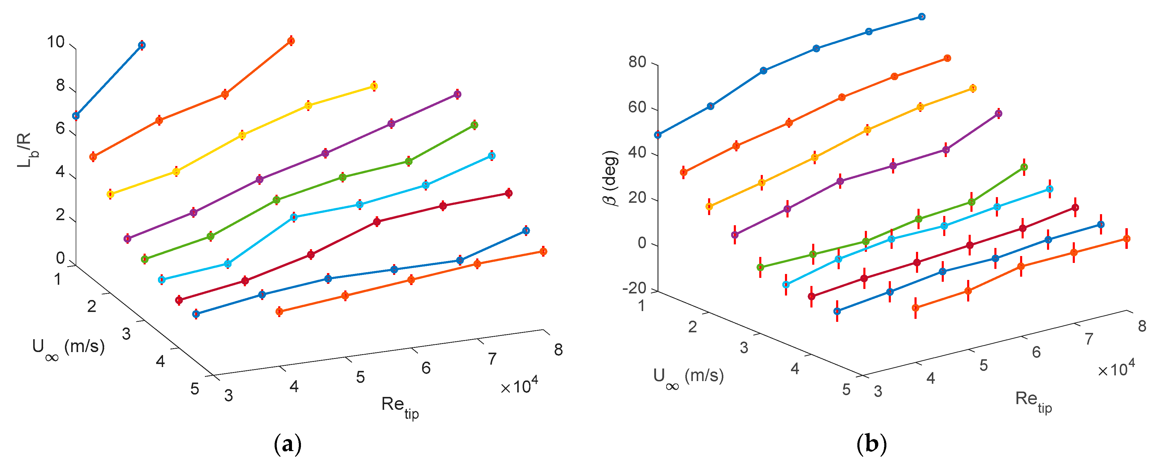
The results from all of the flow visualization experiments are shown in Figure 6. Each forward flight speed, 1–5 m/s in 0.5 m/s increments, is considered with varying Retip values, 3 × 10⁴–8 × 10⁴ in 1 × 10⁴ increments, leading to an advance ratio range of 0.04–0.54. The disturbance distance below the multi-rotor, is shown in Figure 6a for different freestream speeds under consideration with varying Retip values with error bars, again based on 10-pixel uncertainty. Clearly, as is increased, the distance the wake disturbance propagates below the multi-rotor UAV decreases. As expected, as the rotor speed is increased, the disturbance distance increases. The error bars presented in Figure 6a are small compared to the overall scale of the plot being presented. The 10-pixel uncertainty under consideration is almost negligible when considering the full scale of observed over the full range of advance ratios. As the is increased, is substantially reduced, as seen in Figure 6b. Alternatively, as the rotor speed is increased for a constant , increases but is not as sensitive as in the case of a change in . Furthermore, at 2.5 m/s, approaches a constant value that is dependent on Retip. The errors in the jet angle are more considerable at low jet angles, as seen previously, but for the higher jet angles, the 10-pixel uncertainty is rather negligible. The trends seen in and are strikingly similar as expected given In both cases, different combinations of freestream speeds and rotor speeds result in similar outcomes which indicates that is dependent on the ratio of freestream speed to rotor speed, which is taken into account in the advance ratio.
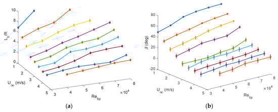
Figure 6.
(a) Disturbance distance, ; and (b) jet angle, for varying freestream speeds, and varying Retip values.
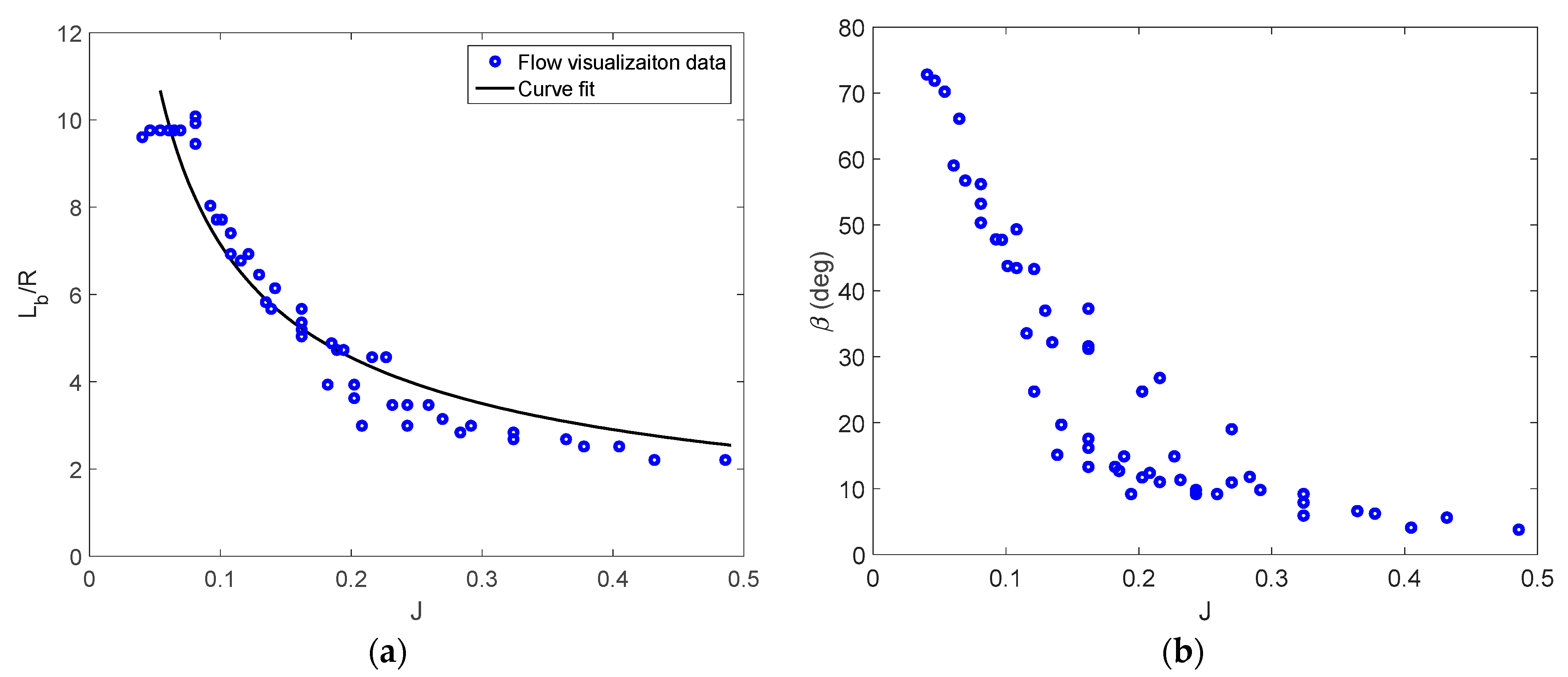
The dependency of and on the advance ratio is clearly seen in Figure 7 where the results from Figure 6 of several experiments with varying and Retip collapse to a single curve that predict and as a function of . In Figure 7a, as increases, sharply decreases from the maximum value of 10 for 0.1 and approaches 2.5 for 0.2. From the data, a function for the disturbance distance as a function of the advance ratio, , is considered and shown in solid black in Figure 7a. This data fit can be used to influence sensor placement or predict potential proximity effects. A similar trend is observed in Figure 7b, where decreases from a maximum value of 75° for low and approaches a constant of ~10° for 0.2. In both figures, as the advance ratio exceeds 0.2, further increases do not yield as drastic of a change in either the or , as was indicated in Figure 4. Error bars are omitted in Figure 7 for clarity as they make the results difficult to see and have been shown previously.
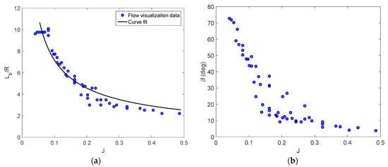
Figure 7.
(a) Disturbance distance, ; and (b) jet angle, for varying advance ratios.
In addition to below the multi-rotor UAV’s body, during forward flight there is also a disturbance above the body as depicted in Figure 8a,b which show flow visualization above the UAV for = 1 m/s and Retip = 3 × 10⁴ ( = 0.11) and Retip = 8 × 10⁴ ( = 0.04), respectively. In each case, there is a deflection of the streamlines closest to the multi-rotor UAV as the freestream flow is pulled into the rotors. At the lower rotor speed, Figure 8a shows that although all of the streamlines above the vehicle are affected, in comparison to a higher rotor speed as shown in Figure 8b, they are less modified.
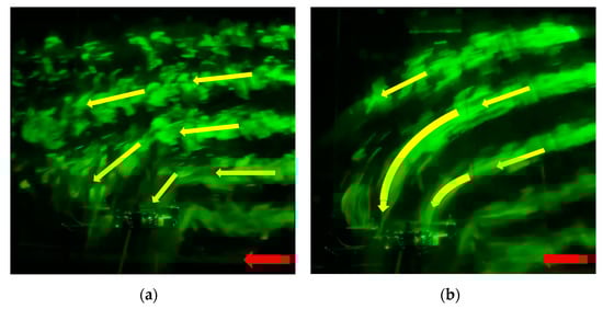
Figure 8.
Flow visualization results above the multi-rotor UAV in forward flight at = 1 m/s and (a) Retip = 3 × 10⁴ ( = 0.11) and (b) Retip = 8 × 10⁴ ( = 0.04).
As the flight speed increases, the rotors have less of an effect on the flow above the multi-rotor UAV which can be seen in Figure 9a,b where Retip = 8 × 10⁴ and is increased to 3 m/s (= 0.12) and 5 m/s ( = 0.20), respectively. At = 0.20, only the nearest streamline to the multi-rotor UAV is significantly deflected into the rotors. Additionally, the upper streamline within the FOV remains nearly parallel to the background flow, showing little signs of modification caused by the rotors. This shows that, even at high rotor speeds, is able to dominate the flow and the flow above the UAV remains relatively unaffected. A preliminary conclusion that can be drawn from this is that above the multi-rotor UAV is the optimal location for integration of in-situ instrumentation, especially when the unmanned vehicle is operated at 0.20.
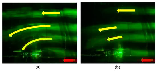
Figure 9.
Flow visualization results above the multi-rotor UAV in forward flight at Retip = 8 × 10⁴ for freestream speeds of (a) = 3 m/s ( = 0.12) and (b) = 5 m/s ( = 0.20).
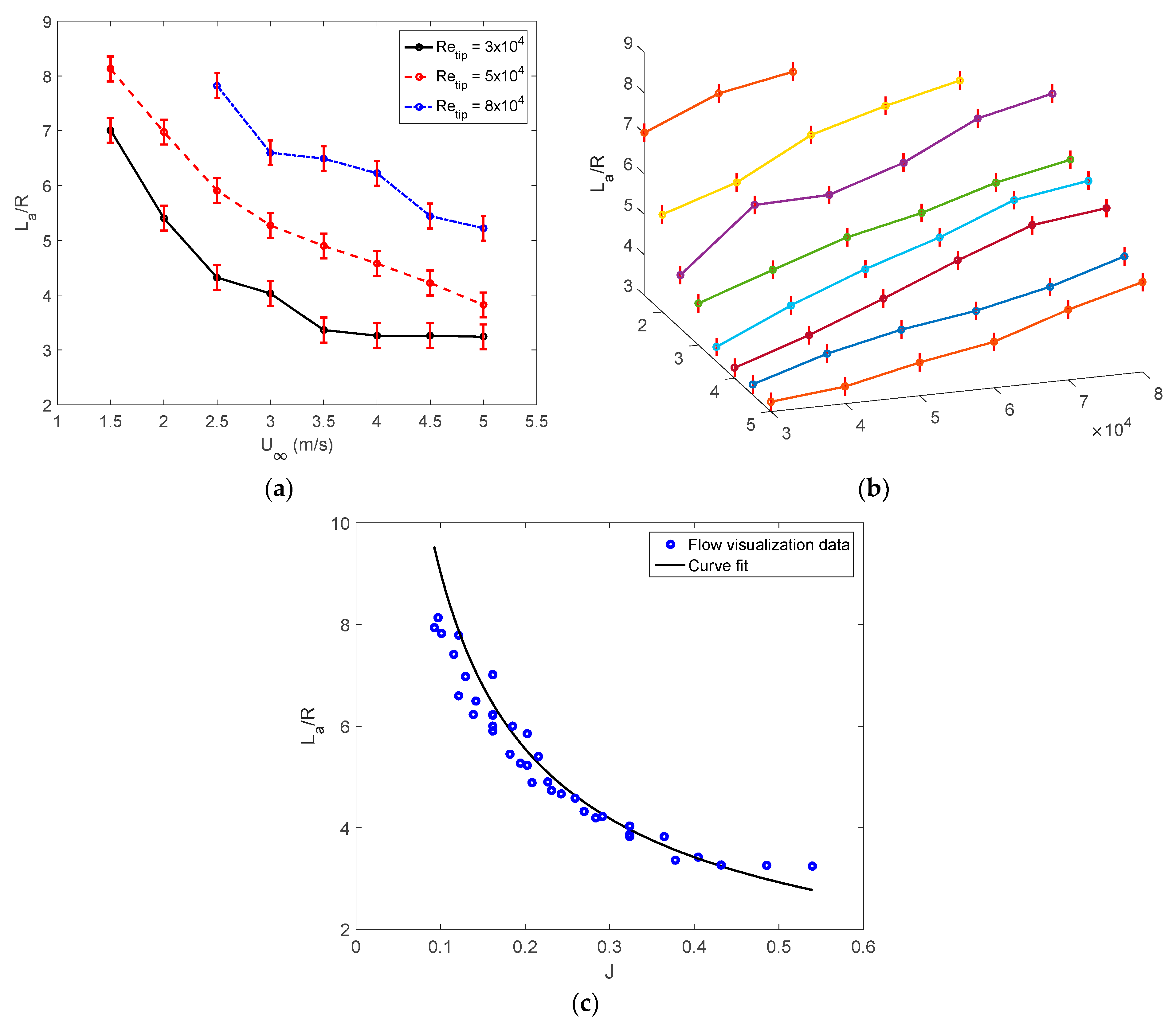
The distance above the multi-rotor vehicle where the flow returns to , can be estimated from the flow visualization results. In Figure 10a, , is plotted versus for three Retip considerations. It should be noted that < 1.5 m/s is not presented in the plots as extends beyond the illuminated FOV and an accurate estimation of disturbance distance cannot be obtained. Low values of result in measurable disturbances at distances of up to 8 above the multi-rotor, even for low Retip. As is increased, decreases for each Retip and approaches a constant value as it becomes independent on . Figure 10 shows the trend of versus both and Retip, with 10-pixel uncertainty error bars. As Retip is increased, increases for a constant , which is expected as more of the incoming flow is pulled into the rotors. As previously mentioned, and Retip can be simultaneously described through the advance ratio, . Figure 10c depicts versus the where as is increased, is decreased and approaches a constant value of approximately 3 for 0.35. The disturbance distance above the multi-rotor UAV can be expressed as , shown as a black solid line in Figure 10c. As previously mentioned, this expression can be used to determine where to place in-situ instrumentation and predict proximity effects on a multi-rotor UAV.
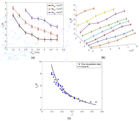
Figure 10.
Disturbance distance, , versus (a) , (b) and Retip, and (c) from the flow visualization experiments.
Table 1 presents the values for Lb/R and La/R at J = 0.10 and J = 0.55, in addition to the range of the disturbance distances over this range of advance ratios, based on the expressions derived from the flow visualization data. At low advance ratios, there is a greater disturbance predicted above the multi-rotor UAV which more rapidly reduces. At high advance ratios, the disturbance distances above and below the multi-rotor vehicle are relatively similar, resulting in a larger range for La/R. Clearly, the disturbance distance above the multi-rotor UAV is more sensitive to changes in the advance ratio. Additionally, if in-situ instrumentation is to be integrated onto the multi-rotor, it should be placed well outside of the wake and the UAV should be flown at high advance ratios to avoid corrupting data collected by the instrumentation.

Table 1.
Lb/R and La/R at J = 0.10 and J = 0.55, and their corresponding ranges based on flow visualization expression.
3.2. PIV Results
Based on the results from the flow visualization experiments, it is clear that both and rotor speed () have large impacts on multi-rotor UAV rotor–wake interactions and the corresponding disturbance distances (). The effect of each of these parameters is captured through advance ratio, therefore 10 advance ratios are considered for PIV testing. Since PIV experiments are more resource intensive—including setup, experimentation, and data processing—a range of advance ratios similar to the considered flow visualization parameters are considered in order to capture a wide array of flight conditions. Table 2 shows the considered advance ratios and the corresponding wind tunnel and rotor speeds. The advance ratios encountered during operation are dependent on the design and the mission; however, the presented range of advance ratios can be used to inform designers and users in addition to being used to obtain a general understanding of wake propagation in forward flight.
Table 2.
Considered advance ratios and corresponding flight parameters.
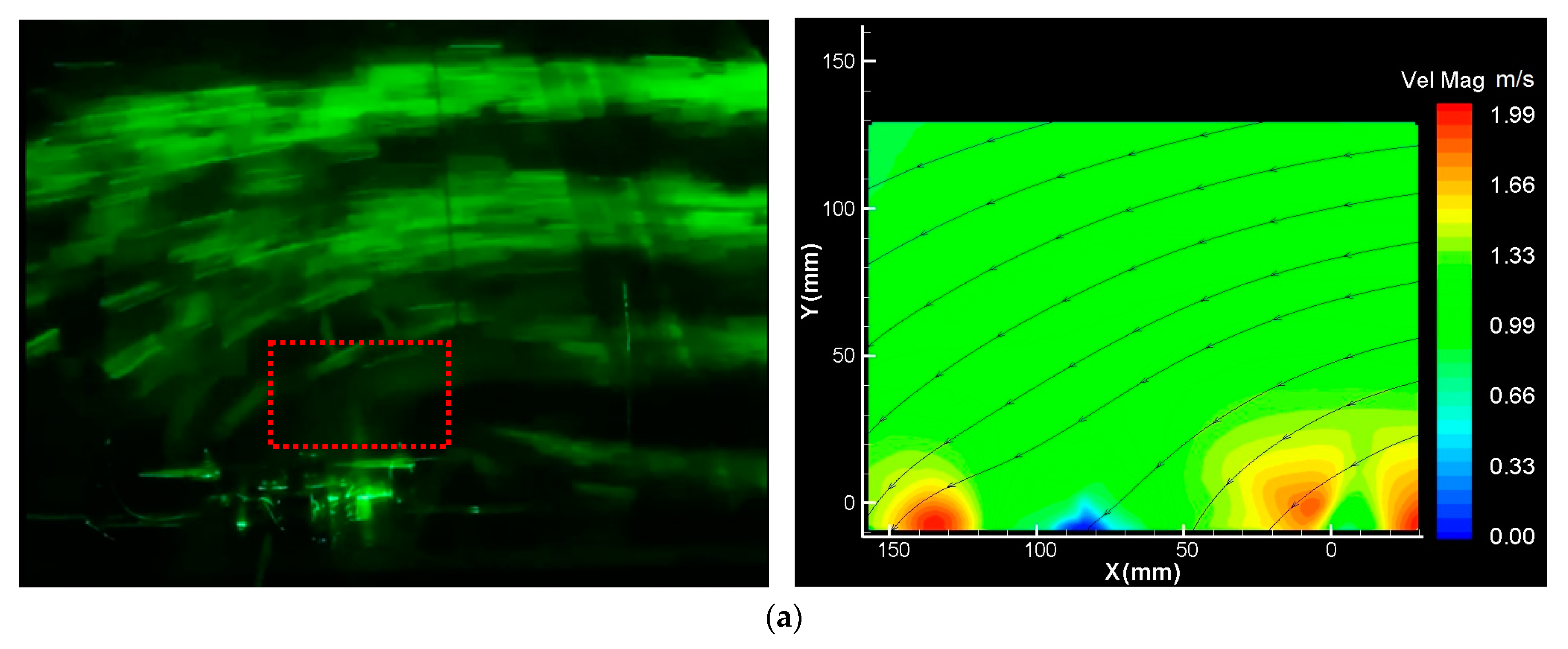
Unlike flow visualization, to obtain high-resolution quality PIV results, the size of the FOV is much more limited. Based on this, results from the flow visualization experiments are used to determine the optimal FOV location for the PIV experiments. Figure 11a,b shows the FOV designated by the red box for forward flight PIV experiments that was focused below and above the body of the multi-rotor UAV respectively. Both FOVs are selected to capture the detailed flow field in the vicinity of the body.

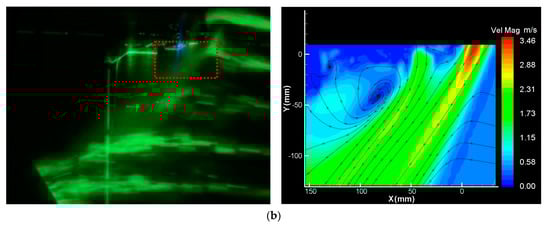
Figure 11.
FOV comparison for forward flight PIV and flow visualization experiments (a) below and (b) above the multi-rotor UAV.
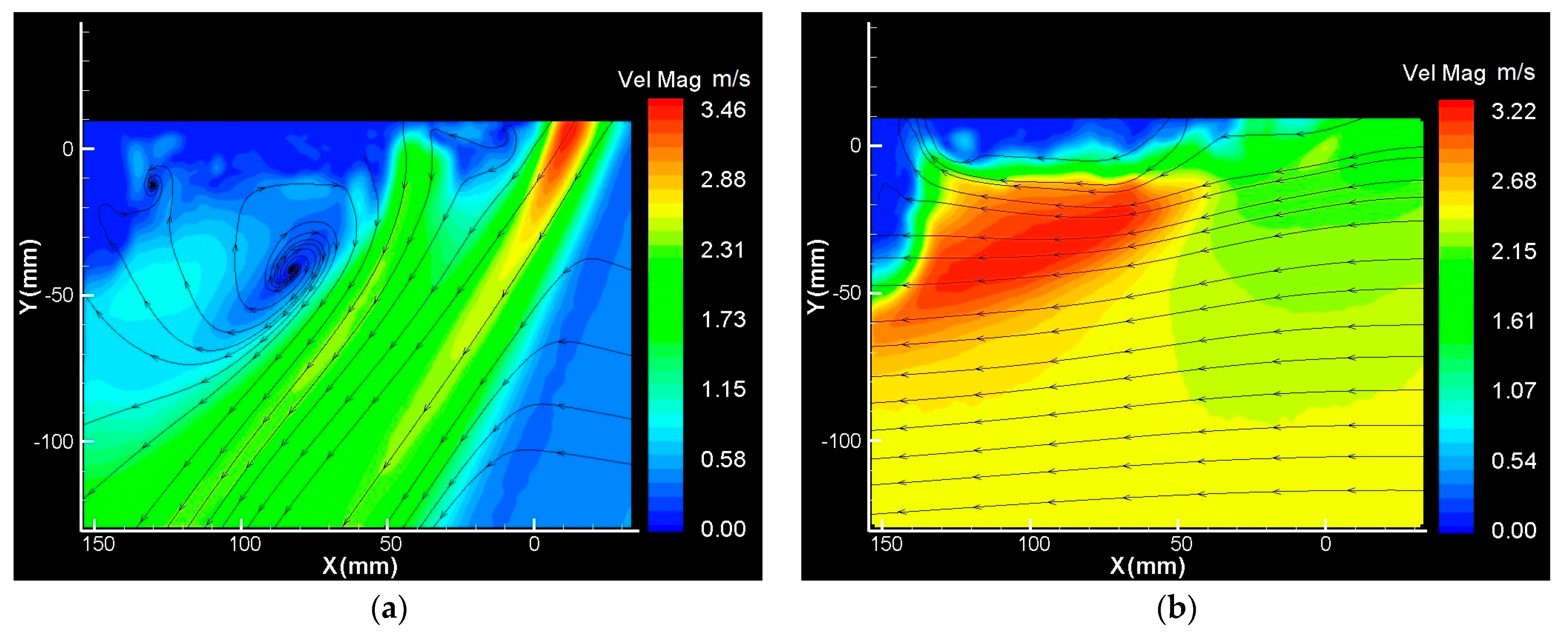
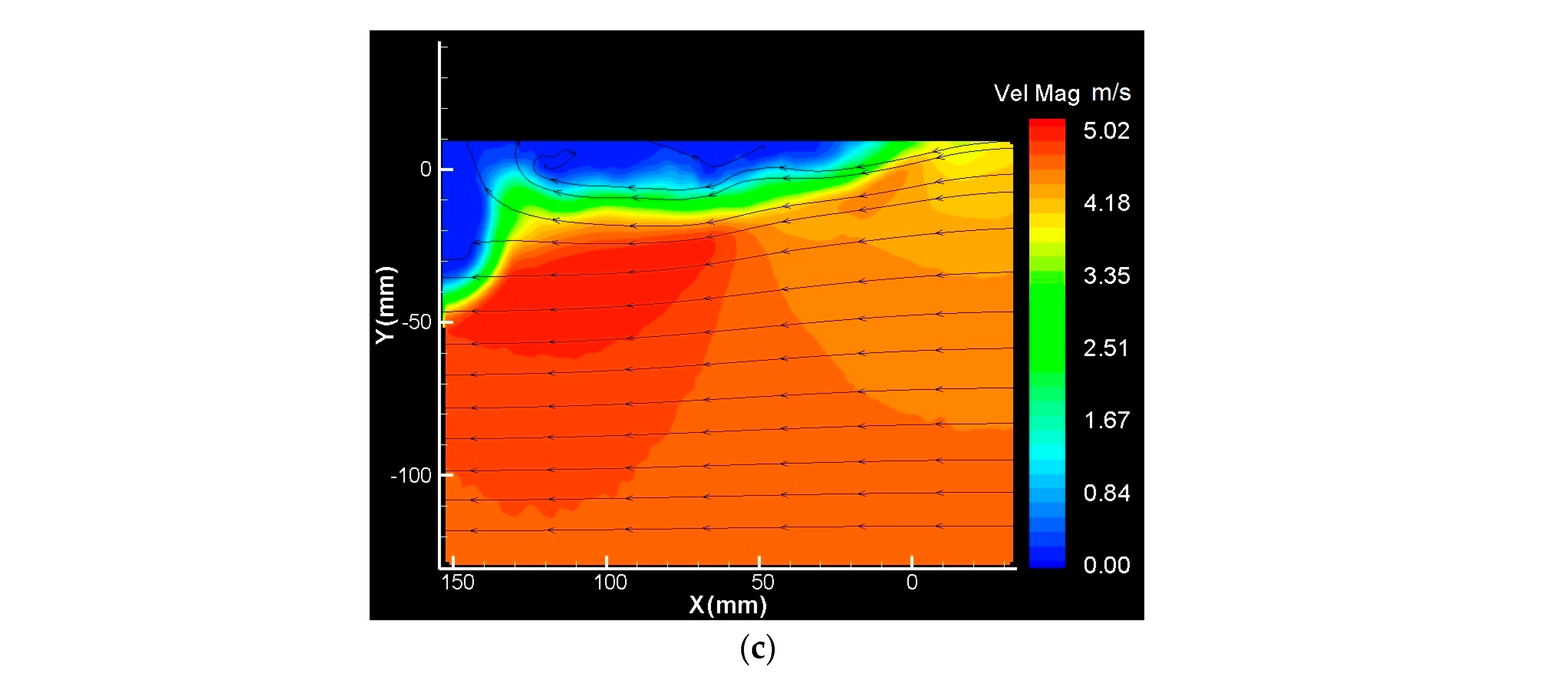
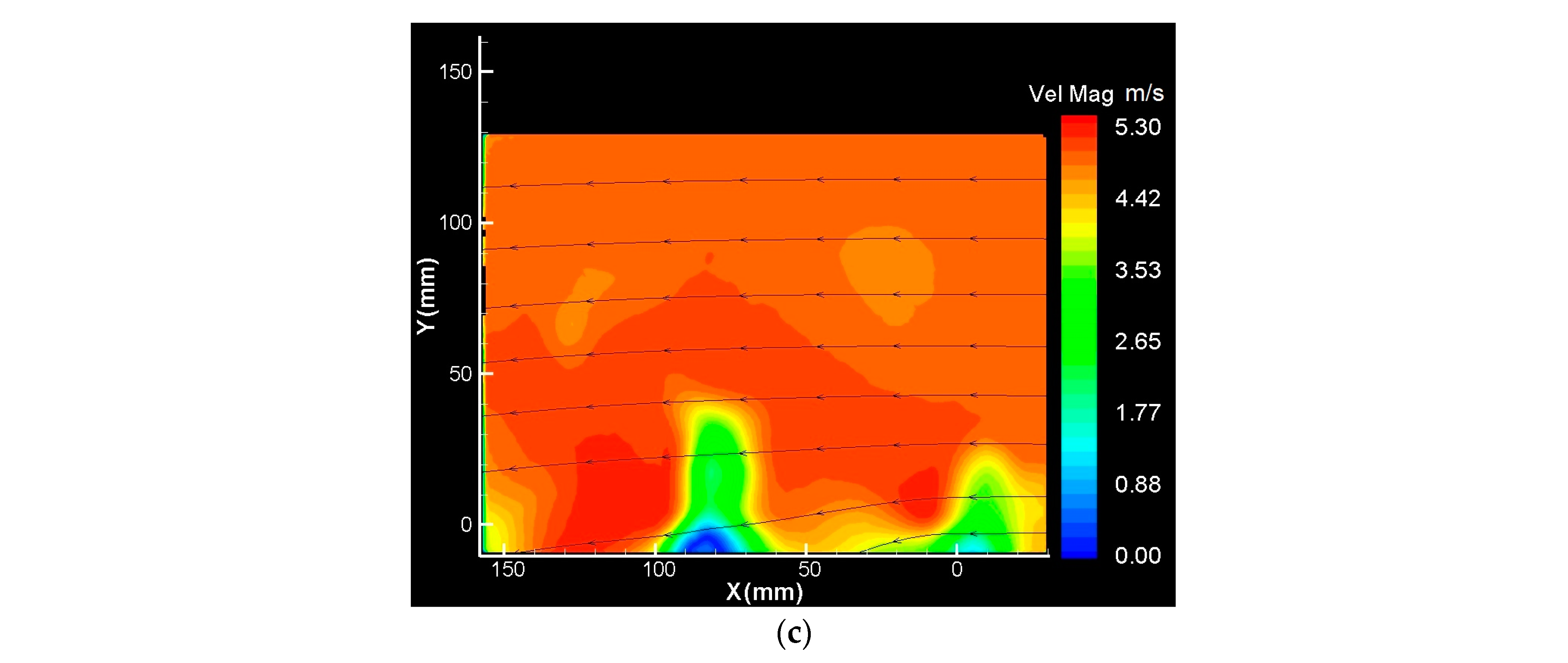
As can be seen from Table 2, higher advance ratios are generally achieved in the experiments with higher (flight speed) while keeping relatively constant, which results in dominating the flow around the body of the UAV, while at lower advance ratios, the rotor jets tend to dominate the flow and there is considerable disturbance that extends beneath it. As increases, the rotor jets become less dominant and is reduced. Figure 12a shows the PIV results below the multi-rotor UAV for = 0.09 and a jet is clearly visible that is expelled from the front rotors. Due to the limited extent of the FOV, the location where the flow returns to cannot be determined. In addition, there is an evident recirculation zone directly beneath the body of the multi-rotor UAV which was not visible from the flow visualization experiments. As is increased to 0.24, as shown in Figure 12b, there is still a clear area of elevated velocity below the multi-rotor, but the rotor jet observed in Figure 12a is much less discernable and is more reminiscent of bluff body flow. In this case, the flow within the FOV approaches the inlet state farther away from the multi-rotor, but streamlines throughout the FOV are modified by the rotor wake, although minimal at the outer extent. Lastly, at = 0.54, as depicted in Figure 12c, the flow further resembles bluff body flow with a clear deficit near the multi-rotor, surrounded by a shear layer, and then the flow returns to at ~ 0.. In summary, when multi-rotors are operated at higher advance ratios, in situ instrumentation can be mounted closer to the body (as low as around 0.8 for the extreme case of = 0.54) and the chance of ground effect on the vehicle is greatly reduced.

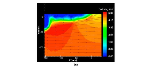
Figure 12.
PIV results below the multi-rotor UAV in forward flight for (a) = 0.09, (b) = 0.24, and (c) = 0.54.
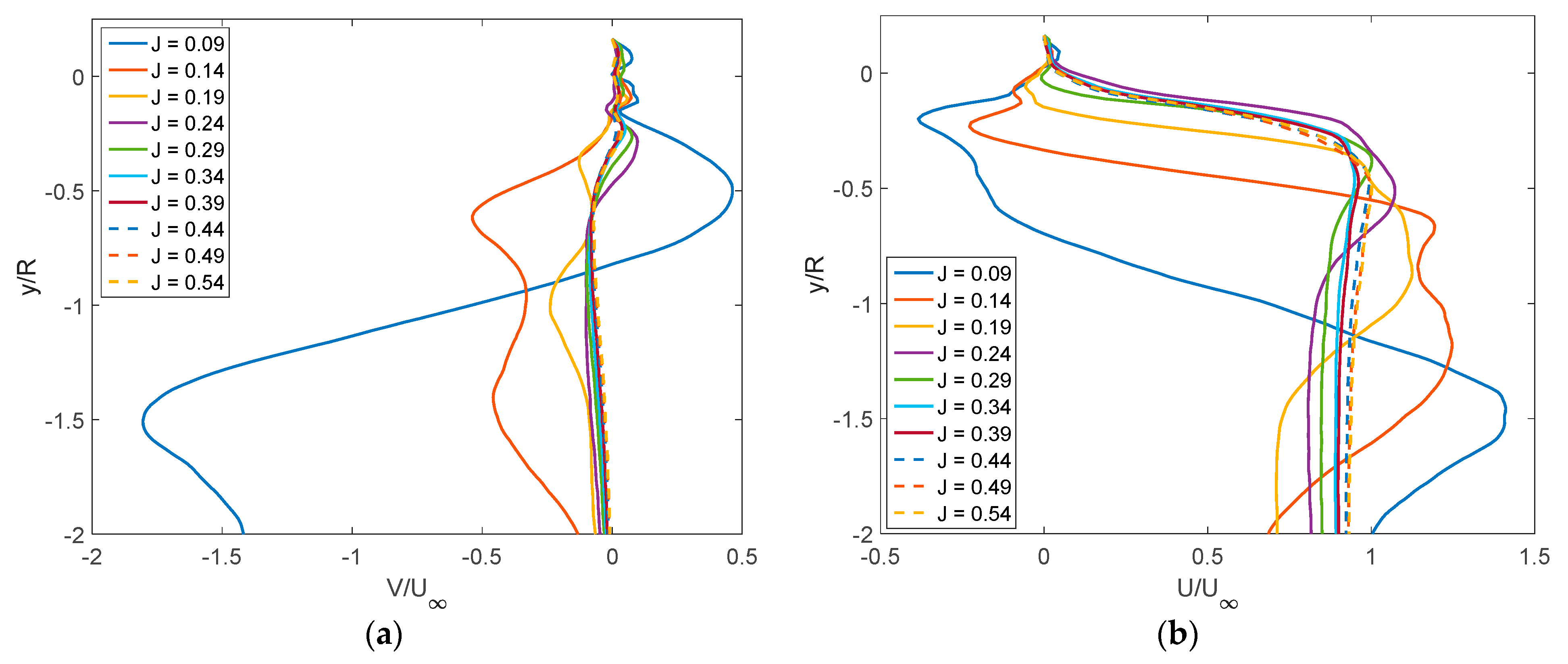
Below the multi-rotor UAV, as shown in Figure 12, the flow exhibits drastic velocity changes throughout the FOV that are associated with the interaction of the rotor jets with the background flow. Figure 13a shows the vertical velocity, at x = 92 mm, for varying . This location is selected as it is in the center of the multi-rotor UAV, which is the ideal location for stability for most in-situ sensors. At higher advance ratios, is not significant. Alternatively, low advance ratios show significant deviations in that trends towards 0 as the distance from the multi-rotor UAV increases. In particular, the = 0.09 case exhibits 0 in the recirculation zone seen in Figure 12a and then passes through a shear layer at ~−1 at which point 0 in the rotor jet region. This case is somewhat unique in that is the only that has a recirculation zone. Figure 13b shows the horizontal velocity, versus the vertical distance from the multi-rotor, , for varying , at the same location = 92 mm. Once again, low cases exhibit complex flow behavior characterized by an extended region of velocity deficit directly below the multi-rotor UAV followed by strong shear and the formation of a horizontal jet where the flow is accelerated before returning to the background flow conditions. As approaches 0.24, the flow converges to a profile that has a clear velocity deficit immediately below the multi-rotor UAV that extends downward 0.5 before approaching a constant of throughout the remainder of the FOV. This may be a result of blockage in the tunnel or could be a consequence of the limited FOV in the PIV experiments. Experiments run in an open tunnel environment or CFD simulations could prove useful in determining the true reason for this phenomenon.
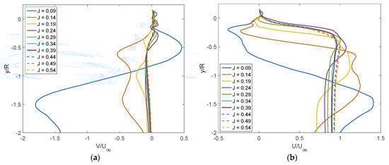
Figure 13.
(a) Vertical velocity, ; and (b) the horizontal velocity, U/ below the center of the multi-rotor UAV ( = 92 mm), with respect to .
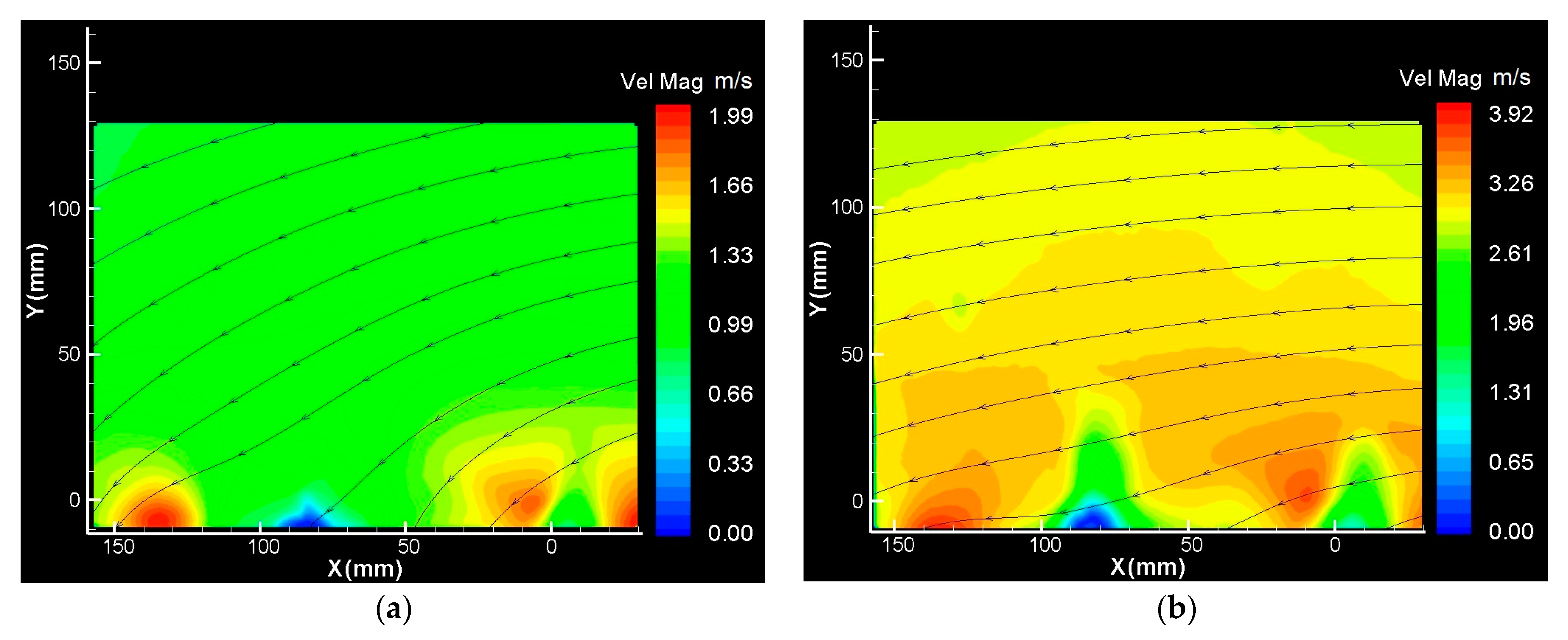
As mentioned previously, alongside the obvious disturbance below the multi-rotor, there is a more subtle modification of the flow above the multi-rotor UAV as air is pulled into the rotors. Although this was observed in the flow visualization, PIV is required to obtain detailed observations of the flow field in the vicinity of the multi-rotor UAV. To accomplish the PIV measurements, the multi-rotor vehicle is mounted upside down in the tunnel test-section to provide sufficient laser illumination of the FOV. For low advance ratios such as = 0.09, as presented in Figure 14a, the streamlines are deflected throughout the FOV. As is increased to 0.24, as shown in Figure 14b, the streamlines within the FOV are not as significantly affected; however, they are still deflected throughout the FOV. For the extreme case tested in this study, = 0.54, the flow returns to at ~ 0.8, as depicted in Figure 14c. Near the multi-rotor, inconsistent and low velocity regions can be seen for all cases, but they become more prevalent as increases. These low-velocity regions are not physical and are caused by reflections off of the motors and body of the multi-rotor UAV.
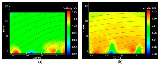
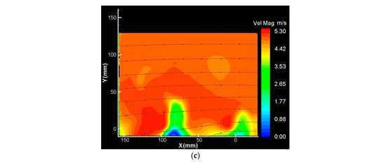
Figure 14.
PIV results above the multi-rotor UAV in forward flight for (a) = 0.09, (b) = 0.24, and (c) = 0.54.
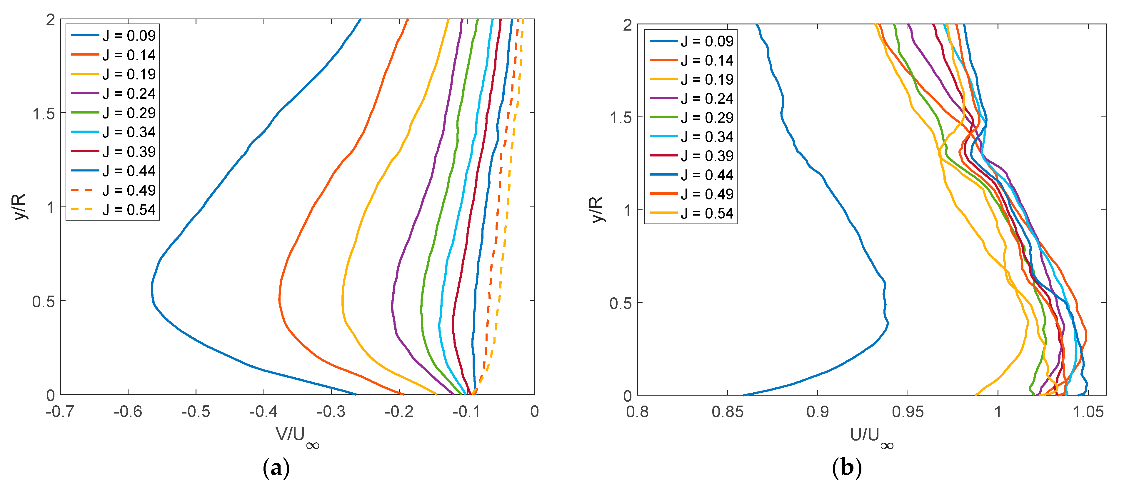
Flow visualization and PIV experiments show that below the multi-rotor UAV is a much less suitable location for integrated in-situ sensors compared to the top of the multi-rotor UAV. Furthermore, directly above the center of the multi-rotor UAV is an ideal location in order to minimize flow disturbance and maintain vehicle stability during operation. This does not suggest that the area above the multi-rotor UAV is absent flow disturbance, rather that it is minimized there. To obtain accurate velocity sensor data, the velocity components require correction as shown in Figure 15a,b where and are plotted, respectively, for various versus the vertical distance from the multi-rotor, , at x = 100 mm. In Figure 15a, as is increased, a drastic reduction in is observed, further suggesting the multi-rotor UAV should be operated at higher to reduce errors in in situ sensor velocity measurements. In this range of 0.24, for a given , is nearly constant over making the velocity correction rather simple. At 0.24, exhibits a stronger dependency on and large gradients near the multi-rotor UAV. In contrast as shown in Figure 15b, is nearly constant throughout the FOV, differing by only around 5% in most cases with the exception of the = 0.09 case which shows a significant deviation from and high dependency on . This deviation is likely due to a transition of regimes at 0.14, where the balance of momentum tips from the freestream towards the rotor jets.
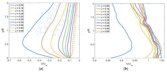
Figure 15.
(a) Vertical velocity, ; and (b) the horizontal velocity, U/ above the center of the multi-rotor UAV ( = 100 mm), with respect to .
PIV is able to provide quantitative data that are not obtained from running flow visualization experiments alone. The velocity profiles provided in Figure 13 and Figure 15 can be used to determine velocity correction factors for instrumentation integrated onto the multi-rotor vehicle. Although PIV provides useful information in the form of more accurate velocity measurements, its limited FOV is a clear drawback and indicates the usefulness of flow visualization experiments. The increased FOV of flow visualization experiments allows disturbance distances to be determined. If only PIV experiments were carried out, the disturbance distances could not be found as they are over 2R below and above the multi-rotor UAV and would therefore not be contained in the PIV FOV. As they do not require post-processing and are easier to set up, flow visualization experiments can be carried out quicker and they do not require excessive storage space. In order to obtain disturbance distances from PIV experiments, more simulations would need to be run with varying FOVs to cover the full space that is captured through flow visualization. This would require an excessive amount of time and data to accomplish making it much less efficient than flow visualization techniques. As the results of the flow visualization and PIV are both useful, it is recommended to use both strategies to obtain disturbance distances over a large FOV while obtaining accurate velocity data near the multi-rotor vehicle which can provide velocity correction factors.
4. Conclusions
Multi-rotors continue to be used for a wide variety of commercial, industrial, and hobby applications due to their availability, utility, and ease of use. For many applications, the wake from the multi-rotor UAV can have a negative effect on the performance or its intended application. The wake can initiate proximity effects or cause inaccurate in situ sensor data. It is crucial for the wake from multi-rotors to be accurately modeled to allow designers and users to make accurate predictions of the wake to ensure accurate sensor data and safe operation. In this study, wind tunnel investigations were used to study the wake from a multi-rotor UAV in forward flight. First, flow visualization experiments were carried out for a variety of wind tunnel speeds and rotor speeds to gain a visual understanding of the wake characteristics above and below the multi-rotor UAV. Although flow visualization experiments did not provide quantitative data, they were used to influence PIV experiments to include flight parameters and FOV. Flow visualization results showed that low freestream speeds and high rotor velocities cause strong wakes below and above the multi-rotor UAV. As freestream speed is increased or rotor speed is decreased, the wake is not as strong as the freestream flow dominates. Using flow visualization experiments, disturbance distances above and below the UAV were estimated. In addition, the jet angle expelled from the rotors was estimated. Using the estimations for disturbance distance, expressions were determined to help designers and users predict the wake effects from other multi-rotors to influence sensor placement and predict proximity effects. Based on results from flow visualization, PIV experiments were carried out looking above and below the multi-rotor vehicle for a wide range of advance ratios, a dimensionless parameter proportional to freestream speed, and inversely proportional to rotor speed. As the advance ratio is increased, the wake does not propagate as far beneath the UAV and returns to parallel to the background flow. For 0.2, the disturbance below the multi-rotor UAV reaches a constant value of 2.5R, after which the flow returns to the background flow state. In addition, higher advance ratios exhibit less disturbance above the multi-rotor, reaching a constant value of approximately 3R for 0.35. Using PIV data, horizontal and vertical velocities were determined above and below the center of the multi-rotor UAV. For 0.24, PIV results showed that flow reaches a somewhat constant state that does not vary with further increasing the advance ratio, looking below the multi-rotor UAV. Operating at high advance ratios reduces the disturbance above the unmanned vehicle, making it the ideal location for in-situ instrumentation as below the vehicle exhibits more unpredictable behavior. Velocity corrections above the multi-rotor UAV show that the vertical velocity component is changed for varying advance ratios, but the effect is minimized as the advance ratio is increased. Alternatively, looking above the multi-rotor, only J = 0.09 exhibits a small horizontal velocity gradient but the rest of the considered advance ratios differ by only about 5%. The PIV results compared well to flow visualization results and confirm that higher advance ratios will minimize the ground and ceiling effects and allow the user to mount in situ sensors closer to the body of the multi-rotor UAV.
Author Contributions
Conceptualization, G.T., A.A. and C.M.H.; methodology, G.T., A.T., C.M.H. and A.A.; software, G.T., A.T. and F.S.; formal analysis, G.T., A.T., C.M.H., F.S. and A.A.; investigation, G.T., A.T., C.M.H. and A.A.; resources, F.S. and A.A.; data curation, G.T. and A.T.; writing—original draft preparation, G.T.; writing—review and editing, A.T., C.M.H., F.S. and A.A.; visualization, C.M.H. and A.A.; supervision, C.M.H. and A.A.; project administration, A.A.; funding acquisition, C.M.H. and A.A. All authors have read and agreed to the published version of the manuscript.
Funding
This research was funded by US Army Research Laboratory.
Institutional Review Board Statement
Not applicable.
Informed Consent Statement
Not applicable.
Acknowledgments
The authors G. Throneberry and A. Abdelkefi would like to acknowledge the financial support from the US Army Research Laboratory.
Conflicts of Interest
The authors declare no conflict of interest.
References
- Hassanalian, M.; Abdelkefi, A. Classifications, applications, and design challenges of drones: A review. Prog. Aerosp. Sci. 2017, 91, 99–131. [Google Scholar] [CrossRef]
- Gupta, S.G.; Ghonge, M.M.; Jawandhiya, P.M. Review of unmanned aircraft system (UAS). Int. J. Adv. Res. Comput. Eng. Technol. (IJARCET) 2013, 2, 1646–1658. [Google Scholar] [CrossRef]
- Darvishpoor, S.; Roshanian, J.; Raissi, A.; Hassanalian, M. Configurations, flight mechanisms, and applications of unmanned aerial systems: A review. Prog. Aerosp. Sci. 2020, 121, 100694. [Google Scholar] [CrossRef]
- Vergouw, B.; Nagel, H.; Bondt, G.; Custers, B. Drone technology: Types, payloads, applications, frequency spectrum issues and future developments. In The Future of Drone Use; TMC Asser Press: The Hague, The Netherlands, 2016; pp. 21–45. [Google Scholar]
- Charavgis, F. Monitoring and Assessing Concrete Bridges with Intelligent Techniques. Doctoral Dissertation, Delft University of Technology, Delft, The Netherlands, 2017. [Google Scholar]
- Rakha, T.; Gorodetsky, A. Review of Unmanned Aerial System (UAS) applications in the built environment: Towards automated building inspection procedures using drones. Autom. Constr. 2018, 93, 252–264. [Google Scholar] [CrossRef]
- Irizarry, J.; Gheisari, M.; Walker, B.N. Usability assessment of drone technology as safety inspection tools. J. Inf. Technol. Constr. 2012, 17, 194–212. [Google Scholar]
- Ashour, R.; Taha, T.; Mohamed, F.; Hableel, E.; Kheil, Y.A.; Elsalamouny, M.; Cai, G. Site inspection drone: A solution for inspecting and regulating construction sites. In Proceedings of the IEEE 59th International Midwest Symposium on Circuits and Systems (MWSCAS), Abu Dhabi, United Arab Emirates, 16–19 October 2016; pp. 1–4. [Google Scholar]
- Kalaitzakis, M.; Vitzilaios, N.; Rizos, D.C.; Sutton, M.A. Drone-based StereoDIC: System development, experimental validation and infrastructure application. Exp. Mech. 2021, 61, 981–996. [Google Scholar] [CrossRef]
- Canisius, F.; Wang, S.; Croft, H.; Leblanc, S.G.; Russell, H.A.; Chen, J.; Wang, R. A UAV-based sensor system for measuring land surface albedo: Tested over a boreal peatland ecosystem. Drones 2019, 3, 27. [Google Scholar] [CrossRef] [Green Version]
- Reuder, J.; Brisset, P.; Jonassen, M.; Müller, M.; Mayer, S. The Small Unmanned Meteorological Observer SUMO: A new tool for atmospheric boundary layer research. Meteorol. Z. 2009, 18, 141–147. [Google Scholar] [CrossRef]
- Higgins, C.W.; Wing, M.G.; Kelley, J.; Sayde, C.; Burnett, J.; Holmes, H.A. A high resolution measurement of the morning ABL transition using distributed temperature sensing and an unmanned aircraft system. Environ. Fluid Mech. 2018, 18, 683–693. [Google Scholar] [CrossRef]
- Koparan, C.; Koc, A.B.; Sawyer, C.; Privette, C. Temperature profiling of waterbodies with a UAV-integrated sensor subsystem. Drones 2020, 4, 35. [Google Scholar] [CrossRef]
- Jumaah, H.J.; Kalantar, B.; Halin, A.A.; Mansor, S.; Ueda, N.; Jumaah, S.J. Development of UAV-based PM2. 5 monitoring system. Drones 2021, 5, 60. [Google Scholar] [CrossRef]
- Bürkle, A.; Segor, F.; Kollmann, M. Towards autonomous micro uav swarms. J. Intell. Robot. Syst. 2011, 61, 339–353. [Google Scholar] [CrossRef]
- Fradenburgh, E.A. The helicopter and the ground effect machine. J. Am. Helicopter Soc. 1960, 5, 24–33. [Google Scholar] [CrossRef]
- Ganesh, B.; Komerath, N.; Pulla, D.P.; Conlisk, A. Unsteady aerodynamics of rotorcraft in ground effect. In Proceedings of the 43rd AIAA Aerospace Sciences Meeting and Exhibit, Reno, NV, USA, 10–13 January 2005; p. 1407. [Google Scholar]
- Nathan, N.D.; Green, R.B. The flow around a model helicopter main rotor in ground effect. Exp. Fluids 2012, 52, 151–166. [Google Scholar] [CrossRef]
- Robinson, D.C.; Chung, H.; Ryan, K. Numerical investigation of a hovering micro rotor in close proximity to a ceiling plane. J. Fluids Struct. 2016, 66, 229–253. [Google Scholar] [CrossRef]
- Fernando, H.J.S.; Pardyjak, E.R.; Di Sabatino, S.; Chow, F.K.; De Wekker, S.F.J.; Hoch, S.W.; Hacker, J.; Pace, J.C.; Pratt, T.; Pu, Z.; et al. The MATERHORN: Unraveling the intricacies of mountain weather. Bull. Am. Meteorol. Soc. 2015, 96, 1945–1967. [Google Scholar] [CrossRef]
- McAlpine, J.D.; Koracin, D.R.; Boyle, D.P.; Gillies, J.A.; McDonald, E.V. Development of a rotorcraft dust-emission parameterization using a CFD model. Environ. Fluid Mech. 2010, 10, 691–710. [Google Scholar] [CrossRef]
- Cheeseman, I.C.; Bennett, W.E. The Effect of Ground on a Helicopter Rotor in Forward Flight. 1955. Available online: https://reports.aerade.cranfield.ac.uk/handle/1826.2/3590 (accessed on 30 March 2022).
- Bernard, D.D.C.; Giurato, M.; Riccardi, F.; Lovera, M. Ground effect analysis for a quadrotor platform. In Advances in Aerospace Guidance, Navigation and Control; Springer: Cham, Switzerland, 2018; pp. 351–367. [Google Scholar]
- Sanchez-Cuevas, P.J.; Heredia, G.; Ollero, A. Experimental approach to the aerodynamic effects produced in multirotors flying close to obstacles. In Iberian Robotics Conference; Springer: Cham, Switzerland, 2017; pp. 742–752. [Google Scholar]
- Paz, C.; Suárez, E.; Gil, C.; Baker, C. CFD analysis of the aerodynamic effects on the stability of the flight of a quadcopter UAV in the proximity of walls and ground. J. Wind Eng. Ind. Aerodyn. 2020, 206, 104378. [Google Scholar] [CrossRef]
- Paz, C.; Suárez, E.; Gil, C.; Vence, J. Assessment of the methodology for the CFD simulation of the flight of a quadcopter UAV. J. Wind Eng. Ind. Aerodyn. 2021, 218, 104776. [Google Scholar] [CrossRef]
- Ventura Diaz, P.; Yoon, S. High-fidelity computational aerodynamics of multi-rotor unmanned aerial vehicles. In Proceedings of the 2018 AIAA Aerospace Sciences Meeting, Kissimmee, FL, USA, 8–12 January 2018; p. 1266. [Google Scholar]
- Yoon, S.; Diaz, P.V.; Boyd, D.D., Jr.; Chan, W.M.; Theodore, C.R. Computational aerodynamic modeling of small quadcopter vehicles. In Proceedings of the American Helicopter Society (AHS) 73rd Annual Forum, Fort Worth, TX, USA, 9–11 May 2017. [Google Scholar]
- Shen, A.; Zhou, S.; Peng, S. Atmospheric environment detection method based on multi-rotor UAV platform. Int. Arch. Photogramm. Remote Sens. Spat. Inf. Sci. 2018, 42, 67–71. [Google Scholar] [CrossRef] [Green Version]
- Shukla, D.; Komerath, N. Multirotor Drone Aerodynamic Interaction Investigation. Drones 2018, 2, 43. [Google Scholar] [CrossRef] [Green Version]
- Shukla, D.; Hiremath, N.; Patel, S.; Komerath, N. Aerodynamic interactions study on low-Re coaxial and quad-rotor configurations. In Proceedings of the ASME 2017 International Mechanical Engineering Congress and Exposition, Tampa, FL, USA, 3–9 November 2017; p. V007T09A023. [Google Scholar]
- Ramasamy, M.; Leishman, J.G.; Lee, T.E. Flow field of a rotating-wing micro air vehicle. J. Aircr. 2007, 44, 1236–1244. [Google Scholar] [CrossRef]
- Alvarez, E.J.; Ning, A. High-fidelity modeling of multirotor aerodynamic interactions for aircraft design. AIAA J. 2020, 58, 4385–4400. [Google Scholar] [CrossRef]
- Zhou, W.; Ning, Z.; Li, H.; Hu, H. An experimental investigation on rotor-to-rotor interactions of small UAV propellers. In Proceedings of the 35th AIAA Applied Aerodynamics Conference, Denver, CO, USA, 5–9 June 2017; p. 3744. [Google Scholar]
- Shukla, D.; Komerath, N. Low Reynolds number multirotor aerodynamic wake interactions. Exp. Fluids 2019, 60, 77. [Google Scholar] [CrossRef]
- Shukla, D.; Komerath, N. Rotor–duct aerodynamic and acoustic interactions at low Reynolds number. Exp. Fluids 2019, 60, 20. [Google Scholar] [CrossRef]
- Lei, Y.; Bai, Y.; Xu, Z.; Gao, Q.; Zhao, C. An experimental investigation on aerodynamic performance of a coaxial rotor system with different rotor spacing and wind speed. Exp. Therm. Fluid Sci. 2013, 44, 779–785. [Google Scholar] [CrossRef]
- Jaroslawski, T.; Forte, M.; Moschetta, J.M.; Delattre, G.; Gowree, E.R. Characterisation of boundary layer transition over a low Reynolds number rotor. Exp. Therm. Fluid Sci. 2021, 130, 110485. [Google Scholar] [CrossRef]
- Voutsinas, S.G.; Rados, K.G.; Zervos, A. On the effect of the rotor geometry on the formation and the development of its wake. J. Wind Eng. Ind. Aerodyn. 1992, 39, 283–291. [Google Scholar] [CrossRef]
- Throneberry, G.; Hocut, C.M.; Abdelkefi, A. Multi-rotor wake propagation and flow development modeling: A review. Prog. Aerosp. Sci. 2021, 127, 100762. [Google Scholar] [CrossRef]


Publisher’s Note: MDPI stays neutral with regard to jurisdictional claims in published maps and institutional affiliations. |
© 2022 by the authors. Licensee MDPI, Basel, Switzerland. This article is an open access article distributed under the terms and conditions of the Creative Commons Attribution (CC BY) license (https://creativecommons.org/licenses/by/4.0/).