Abstract
Dengue fever remains a major global health threat, and mathematical models are crucial for predicting its spread and evaluating control strategies. This study introduces a highly flexible dengue transmission model using a novel piecewise fractional derivative framework, which can capture abrupt changes in epidemic dynamics, such as those caused by public health interventions or seasonal shifts. We conduct a rigorous comparative analysis of four widely used but distinct mechanisms of disease transmission (incidence rates): Harmonic Mean, Holling Type II, Beddington–DeAngelis, and Crowley–Martin. The model’s well-posedness is established, and the basic reproduction number () is derived for each incidence function. Our central finding is that the choice of this mathematical mechanism critically alters predictions. For example, models that account for behavioral changes (Beddington–DeAngelis, Crowley–Martin) identify different key drivers of transmission compared to simpler models. Sensitivity analysis reveals that vector mortality is the most influential control parameter in these more realistic models. These results underscore that accurately representing transmission behavior is essential for reliable epidemic forecasting and for designing effective, targeted intervention strategies.
1. Introduction
Dengue fever, a mosquito-borne viral illness, poses a significant global health challenge, particularly in tropical and subtropical regions []. Mathematical modeling plays a crucial role in understanding its transmission dynamics, predicting outbreaks, and evaluating control strategies [,,]. Traditional compartmental models often employ simple bilinear incidence rates [,], which may not adequately capture the complex interaction dynamics between human and mosquito populations, especially when factors such as saturation effects, preventive measures, or behavioral changes come into play. Consequently, various non-linear incidence rates, including Holling type II [], Beddington–DeAngelis (B–D) [], Harmonic Mean [,], and Crowley–Martin [,], have been proposed to offer more realistic representations of disease transmission.
The four non-linear incidence rates investigated in this study—Harmonic Mean, Holling Type II, Beddington–DeAngelis, and Crowley–Martin—were specifically chosen to represent a spectrum of increasing complexity in transmission dynamics. They are canonical forms widely used in mathematical biology and epidemiology to move beyond the limitations of simple bilinear assumptions. The Harmonic Mean type provides a baseline non-linear model where transmission is limited by the lower abundance of the two interacting populations. The Holling Type II rate introduces the concept of saturation, accounting for limitations in the contact or handling capacity, such as a mosquito’s finite biting rate. Building on this, the Beddington–DeAngelis function incorporates interference or protective behaviors from both susceptible and infectious populations. Finally, the Crowley–Martin type models mutual interference, where the presence of other individuals in both populations can reduce contact rates. By systematically comparing these four well-established functional forms within the same piecewise fractional framework, we can directly assess how these distinct biological assumptions influence epidemic dynamics and control implications, providing a robust basis for model selection.
While classical models provide foundational insights [,], their assumption of bilinear incidence often fails to capture real-world complexities. Consequently, the field has moved toward non-linear incidence rates to better model phenomena like behavioral changes and saturation effects. The Holling type II function, for instance, is widely used to represent a saturating infection rate due to factors like limited vector biting capacity []. More sophisticated forms, such as the Beddington–DeAngelis (B–D) and Crowley–Martin functions, have been proposed to account for mutual interference or protective measures from both susceptible and infectious populations. At the same time, the importance of memory and non-local effects in biological systems has led to the increasing use of fractional calculus. Operators like the Atangana–Baleanu–Caputo (ABC) fractional derivative, with its non-singular Mittag–Leffler kernel, have proven effective in capturing these long-range dependencies in epidemiological models [,,]. However, disease dynamics are rarely static. The initial phase of an outbreak may follow classical patterns, whereas later stages can be influenced by cumulative public health interventions or memory effects, necessitating a more flexible modeling approach. To address this, Atangana and Araz introduced piecewise differential operators, which uniquely combine classical and fractional derivatives over different time intervals []. This “crossover” behavior has been successfully applied to model various real-world phenomena, including other infectious diseases [,], demonstrating its power in capturing temporal shifts in system dynamics.
The piecewise modified Atangana-Baleanu-Caputo (PMABC) operator [] provides this flexibility, allowing for a “crossover” in system behavior. The PMABC fractional operator is a potent analytical tool, with foundational details provided in key references [,,]. Its effectiveness has been demonstrated in modeling various phenomena in the real world and exploring associated crossover behaviors [,]. These studies confirm that employing the PMABC operator yields a deeper understanding of system dynamics, particularly concerning the underlying characteristics of disease progression. Although fractional dengue models and various incidence rates have been studied separately [,], this article presents a comprehensive and novel investigation by integrating these concepts within a unified framework.
Dengue outbreaks are often multiphasic. For instance, an outbreak may start with classical exponential growth, but its dynamics can fundamentally change following a major event, such as the onset of a monsoon season (altering vector breeding sites) or the implementation of a large-scale public health intervention (e.g., city-wide fogging, community cleanup campaigns). After such an event, the transmission dynamics might exhibit memory effects (cumulative impact of vector control) or non-local behavior, which are better captured by fractional derivatives. The PMABC operator is uniquely suited to model this “crossover” in system behavior.
Researchers have integrated various nonlinear interaction terms into biological system models. For example, the concept of saturating interaction rates (like Holling type-II) has been foundational in studies of consumer-resource dynamics [] and has also been applied to investigate strategies for managing disease spread within populations []. Alternative functional responses, such as the Beddington–DeAngelis type incorporating intracellular processing time [] or the Crowley–Martin function accounting for mutual interference [], have been used to model virus lifecycles and compartmental disease progression (SEIR structure), respectively. Analytical attention in these studies often centers on determining conditions for population persistence, equilibrium states of the system, and the potential for cyclic dynamics leading to species elimination [].
Beyond traditional differential equations, noninteger-order calculus provides distinct modeling tools. The dynamics of infectious agents such as the Ebola virus have been explored using fractional derivative definitions, specifically the Grunwald–Letnikov approach, which facilitates efficient analysis of the long-term evolution of the system []. The same fractional methodology (Grunwald–Letnikov) was then utilized to examine the spread characteristics of the COVID-19 pandemic []. In addition, fractional-order frameworks have been applied to understand behavioral patterns, such as smoking habits, using numerical solution techniques based on iterative calculations, spatial segmentation, and truncated memory effects [].
While previous studies have effectively applied fractional calculus to dengue modeling [,] or have compared nonlinear incidence rates within classical integer-order frameworks, a critical gap remains in understanding how these two powerful concepts interact. To our knowledge, no prior study has conducted a systematic comparative analysis of multiple sophisticated incidence functions (Harmonic Mean, Holling Type II, Beddington–DeAngelis, Crowley–Martin) within a piecewise fractional framework.
Our primary and novel contribution is therefore twofold: first, we introduce a dengue model using the PMABC operator, which uniquely captures temporal heterogeneity by allowing a transition from classical to fractional dynamics, reflecting shifts in an epidemic’s evolution. This specific operator enables the model to exhibit classical dynamics initially (up to a time ) and fractional dynamics subsequently, reflecting potential changes in transmission characteristics over the course of an epidemic. Second, by embedding these four canonical incidence rates into this advanced structure, we provide the first direct comparison of how different assumptions about transmission mechanisms (e.g., saturation, behavioral change, and mutual interference) alter key epidemiological outcomes when memory effects are also considered. This integrated approach allows us to disentangle the influence of the incidence function from the memory effects, offering novel insights into model selection and the design of time-dependent control strategies.
2. Description of the Model
The authors of [] studied the transmission dynamics of dengue disease between human and mosquito populations.
with the initial conditions
where the transmission terms are initially defined using standard mass action scaled by the human population size: for mosquito-to-human transmission and for human-to-mosquito transmission. Here, and represent the total constant sizes of the human and mosquito populations, respectively. The total human population is stratified into four epidemiological compartments: susceptible (), exposed (), infectious (), and recovered (). Similarly, the total mosquito population is divided into three compartments: susceptible (), exposed (), and infectious (). The model assumes uniform mixing between the populations, implying that every mosquito has an equal probability of biting any given human host. The per-mosquito biting rate is denoted by b. Disease transmission occurs only from infectious humans () to susceptible mosquitoes () and from infectious mosquitoes () to susceptible humans ().
Let denote the transmission probability from an infectious mosquito to a susceptible human per bite, and let denote the transmission probability from an infectious human to a susceptible mosquito per bite. Consequently, the per capita rate at which susceptible humans acquire infection (the force of infection) is given by . Similarly, the per capita rate at which susceptible mosquitoes acquire infection is . These rates, dependent on the relevant population compartments and transmission probabilities, govern the flux of individuals from susceptible to exposed states in both populations. Individuals in the exposed compartments ( and ) are infected but not yet infectious; they transition to the infectious state ( and ) at rates (human incubation rate) and (mosquito extrinsic incubation rate), respectively. The model considers a single strain of the Dengue virus responsible for all infections.
The parameters are defined as follows:
- The natural death rate of humans;
- The natural death rate of mosquitoes;
- The mosquito-to-human transmission probability per bite;
- The human-to-mosquito transmission probability per bite;
- Recovery rate of humans;
- Recruitment rate of mosquitoes;
- The human incubation rate (inverse of latent period);
- The mosquito extrinsic incubation rate (inverse of latent period);
- The mosquito biting rate.
This study aims to investigate a Dengue model incorporating four distinct types of nonlinear incidence rates to more accurately describe the disease’s evolutionary dynamics. This analysis is conducted within the framework of piecewise-modified ABC fractional derivatives. The resulting model equations can be expressed as follows:
is the piecewise modified fractional derivative of order At time , and
The mathematical framework presented in model (1), visually clarified by the schematic in Figure 1, elucidates the system’s temporal dynamics. These representations detail the interplay between the distinct population groups by defining the specific parameters for transmission, recuperation, and mortality.
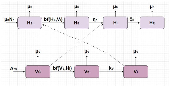
Figure 1.
Flow chart of model (1).
The incidence rate, representing the rate at which new infections occur per unit time, is a critical component of epidemiological models, as it mathematically encodes the assumed mechanism of disease transmission. Understanding its functional form is vital for accurately predicting disease spread. This study explores four distinct non-linear incidence rate formulations, commonly employed in mathematical biology to capture different interaction dynamics beyond simple mass action, often selected based on the specific biological context:
- Harmonic Mean type: This formulation assumes transmission is limited by the less abundant interacting population.
- Holling Type II (Saturated): Proposed by Holling (1959) [], this rate represents saturation in the infection process, e.g., due to limited mosquito biting capacity or handling time, as the density of infectious individuals ( or ) increases. The form for mosquito-to-human transmission iswhere is the saturation constant for infectious mosquitoes. A corresponding form applies for human-to-mosquito transmission, with a saturation constant .
- Beddington–DeAngelis (B–D) type: Introduced independently by Beddington et al. and DeAngelis et al. (1975) [], this rate incorporates density dependence related to both susceptible and infectious populations. The form for mosquito-to-human transmission iswhere reflects inhibition effects due to susceptible human density (e.g., avoidance, protective measures) and represents inhibition/interference among infectious mosquitoes. A corresponding form applies for human-to-mosquito transmission, with coefficients .
- Crowley–Martin type: Proposed by Crowley and Martin [], this form models mutual interference among both interacting populations. The form for mosquito-to-human transmission iswhere are positive constants representing the strength of interference from susceptible humans and infectious mosquitoes, respectively. A corresponding form applies for human-to-mosquito transmission, with constants .
Investigating these different functional forms is crucial, as the choice of incidence rate significantly impacts model dynamics and predictions regarding disease spread and control, potentially addressing limitations in simpler models of Dengue transmission behavior.
The parameters embedded within the model are crucial representations of the diverse biological and epidemiological factors driving Dengue transmission. They encapsulate rates related to disease progression (incubation, recovery), inter-species transmission, vector behavior (biting), and host/vector vital dynamics. The model utilizes these parameters to enable a quantitative exploration of the complex interactions between human and mosquito populations and their influence on the spread of dengue fever.
Crossover Behavior
Epidemiological systems like dengue transmission may exhibit different dynamic characteristics at various stages. To account for such potential temporal heterogeneity, we utilize the piecewise modified Atangana–Baleanu–Caputo (PMABC) fractional operator. This operator structures the model across distinct time segments. Specifically, the total time interval is divided at a designated crossover point . The crossover point, , is intended to represent the precise moment a significant event alters the transmission dynamics, such as the start of a government-mandated vector control program, a documented shift in public awareness and behavior, or a key seasonal change. In the initial segment , corresponding perhaps to the early outbreak phase, the system’s evolution is described by the classical integer-order derivative. For the subsequent segment , the dynamics are governed by the modified ABC (mABC) fractional operator. The rationale for this switch is that phenomena such as long-range memory effects or the cumulative impact of past states (non-local dependencies) might be more effectively captured by fractional calculus in the later stages of disease transmission. The PMABC operator thus explicitly models the crossover behavior, which presents a transition in the governing dynamics from classical to fractional. This hybrid approach, combining the strengths of both classical and fractional derivatives within their respective hypothesized domains of applicability, aims to provide a more nuanced and potentially more accurate description of the complete epidemic trajectory. A crucial aspect of the piecewise framework is the identification of the crossover point , which marks the transition from classical to fractional dynamics. In this theoretical study, was chosen illustratively to demonstrate the model’s capacity to handle such transitions. For practical application to real-world epidemic data, this point would need to be determined rigorously. There are two primary methods for this. The first is through epidemiological justification, where is aligned with a known, significant event that alters transmission dynamics, such as the implementation of a large-scale public health intervention (e.g., lockdowns or vector control programs), a documented shift in population behavior, or a key seasonal change. The second, more data-driven approach is through statistical identification. Here, is treated as a parameter to be estimated. A common technique involves performing a grid search over a range of possible values for . Consequently, the model equations based on (1) take the following piecewise form:
where
- is the crossover point, which presents a transition in the governing dynamics from classical to fractional.
- is the classical derivative of a function
- is MABC fractional derivative defined as
3. Mathematical Properties of the PMABC Model (1)
Here, we discuss some important qualitative behavior of PMABC dengue model (1). Before giving the fundamental properties of the PMABC model (1), we restructure the PMABC model (1) as a compact form as follows:
where and
The integral form of the model (2) is given as follows:
Let be the vector of state variables in the Banach space with the norm
3.1. Lipschitz Property of the Kernels
Theorem 1.
Let Let such that
Then, the Kernels satisfy a Lipschitz conditions with Lipschitz constant where
Proof.
For the Kernel let Then, in the case of Harmonic Mean type and we have
Let . Then Similarly, we can get the following
Let The Kernels satisfy a Lipschitz condition with Lipschitz constant ℓ. In the same manner, we can prove that satisfies a Lipschitz condition with respect to other incidence rates. □
3.2. Existence of Unique Solutions
Theorem 2.
Assume that the Kernel satisfies a Lipschitz conditions with Lipschitz constant defined by Theorem 1. Then, the PMABC dengue model (1) has a unique solution, provided that
Proof.
The existence and uniqueness of the solution for the model (1) are established by applying the Banach Fixed-Point Theorem to the equivalent integral equations. Consider the bounded, forward-invariant, and biologically feasible region defined by
Define an operator as
Let Then, for we have
Next, for we have
By (4) and (5), we have
Thus, the operator is a contraction if . By the Banach Fixed-Point Theorem, the PMABC dengue model (1) has a unique solution in the interval . For more information, see [,]. □
3.3. Boundedness and Positivity of Model (1)
We establish the biological feasibility of the model by showing that solutions starting with non-negative initial conditions remain non-negative (positive) and bounded for all future times.
Theorem 3.
Let the initial conditions be , , , , , , and . Then the solutions of the system (1) remain non-negative for all times .
Proof.
We will prove the non-negativity of each state variable sequentially. From the first equation of the system (1), we have
Let us assume there exists a time such that and for all . At this point, we have
For all standard incidence functions, . Therefore, we have
Since , the rate of change is positive when the population reaches zero, preventing it from becoming negative. Thus, for all . A similar argument holds for , as its equation contains a constant inflow term , ensuring . From the second equation of system (1), we have
Since , , and all parameters are non-negative, the incidence term . This leads to the differential inequality
We analyze this inequality for the two intervals of the PMABC operator.
Case 1: For , the inequality (6) is a classical differential inequality given as
Thus
Since , we have for all .
Case 2: For , applying the Laplace transform to the mABC version of inequality (6) (starting from ) and solving for , then taking the inverse Laplace transform, yields a solution involving the Mittag–Leffler function, which is non-negative for non-negative arguments. This gives
where is the one-parameter Mittag–Leffler function. Since from Case 1 and for real z, it follows that for . Combining both cases, we conclude for all .
The proofs for the remaining compartments follow the same logic.
- For , the equation is . Since we have shown , the inflow term . This leads to the inequality , which, by the same argument as for , implies .
- For , the equation is . With , we get , which implies .
- Similarly, for the vector compartments, having established and :
- -
- The equation for gives the inequality , implying .
- -
- With , the equation for gives , implying .
Since all compartments are shown to be non-negative for all , the solutions of the dengue model (1) are positive and biologically meaningful. This completes the proof. □
Theorem 4.
The solutions of the dengue model (1) are bounded in the biologically feasible region Ω.
Proof.
Let the total human population be and the total vector population be .
Boundedness of the human population : We take the sum of the first four equations of the system (1) to find the rate of change of the total human population:
If we assume that the total human population size in the birth term represents the constant carrying capacity or initial size, and , then . The solution to this fractional differential equation tends toward . Therefore, the human population is bounded. (If is simply a constant influx rate, the argument is slightly different, but boundedness usually holds under realistic parameter assumptions.) Assuming is the constant total population size implies for all . Boundedness of the vector population : Summing the last three equations of model (1), we get
By definition , the inequality (7) becomes
Now, for , we have
Thus, we have
Consequently, is bounded by in case On the other hand, for , we have
We apply the Laplace transform on both sides of (9), and utilizing the asymptotic behavior of the Mittag–Leffler function, we obtain
Thus, in two cases, the solution satisfies
This implies that is bounded. Thus, in two cases, the solution satisfies
This implies that is bounded. □
Since all individual compartments are non-negative and the total populations and are bounded, each compartment is also bounded. Therefore, the solutions of model (1) are bounded and remain within the biologically feasible region
for some K related to (often ) and any , provided the solution starts within . This region is positively invariant.
The proof of boundedness is critical for extending the unique local solution, guaranteed by Theorem 2, to a global solution. For nonlinear fractional systems, the Banach Fixed-Point Theorem directly ensures existence and uniqueness only on a local interval. However, since we have shown that all solutions starting in the compact, forward-invariant region remain within for all times, the solution cannot blow up or develop a singularity in finite time. This allows the unique local solution to be extended for all times . This standard argument establishes the existence of a unique global solution for the model.
4. Comparative Analysis of Nonlinear Incidence Models
4.1. Dengue Model with Harmonic Mean Type Incidence Rate
The model (1) with Harmonic Mean type incidence rate is presented as follows:
4.1.1. Equilibrium Points and Basic Reproduction Number
To find the equilibrium points, we set all fractional derivatives in (10) to zero. In the context of fractional calculus, an equilibrium or steady state is a constant solution, and the Atangana–Baleanu–Caputo derivative of any constant is zero. Therefore, this condition correctly identifies the points where the system’s dynamics cease to change; see []. Setting , we solve for the disease-free equilibrium (DFE):
Thus, the DFE is . We use the next-generation matrix (NGM) method adapted for fractional-order systems to compute . The infected compartments are . The rate of appearance of new infections is given by , and the rate of transfer of individuals between compartments is :
The Jacobians and are computed and evaluated at the DFE .
This implies
The general Jacobian F is
Evaluating at the DFE (where , , , ),
The basic reproduction number is the spectral radius of the next-generation matrix []. Thus, we have
The basic reproduction number is the spectral radius of the next-generation matrix . This calculation yields
4.1.2. Stability of DFE Point
The stability of the DFE for fractional-order systems relates to .
Theorem 5.
The DFE point of the dengue model (10) with fractional order is locally asymptotically stable if , and it is unstable if .
Proof.
The local asymptotic stability of the Disease-Free Equilibrium (DFE), , is determined by the eigenvalues of the Jacobian matrix of the system (10) evaluated at . The DFE is given by . For clarity, let the two incidence functions be
The stability analysis requires the partial derivatives of these functions evaluated at the DFE. The Jacobian matrix J of the system (10), evaluated at the DFE , is given by
This is a block-triangular matrix. The eigenvalues are the entries on the main diagonal of the blocks. The eigenvalues corresponding to the uninfected compartments () are
These eigenvalues are all real and negative. For any fractional order , they satisfy the stability condition .
The stability of the DFE is thus determined by the eigenvalues of the sub-matrix corresponding to the infected compartments . This sub-matrix, which we denote , is given by
The matrix is exactly the matrix derived from the next-generation matrix method, where F describes the rate of new infections and V describes the rate of transitions between infected compartments. For a fractional-order system, the DFE is locally asymptotically stable if all eigenvalues of this sub-matrix satisfy the condition .
This condition is met if and only if the basic reproduction number, defined as the spectral radius of the next-generation matrix, , is less than one. If , then there exists at least one eigenvalue of with a positive real part, which means , rendering the DFE unstable. This concludes the proof. □
4.2. Dengue Model with Holling Type II Incidence Rate
Holling proposed the incidence rate of the form where is the saturation constant. The occurrence of any disease outbreak in Holling type II begins very low and gradually increases with infection. Furthermore, due to the crowding effect, when the number of infected people is very large, the infection reaches a peak. The model (1) with Holling type II incidence rate is presented as follows:
4.2.1. Positivity and Boundedness of Model (11)
Theorem 6.
The solutions of the model (11) starting in the non-negative orthant remain non-negative for all . Furthermore, the solutions are bounded and enter the positively invariant region
for some K related to (often ) and any , provided the solution starts within . This region is positively invariant.
Proof.
Positivity is shown by verifying that on the boundary planes of , the vector field points into or is tangent to . For instance, if , . This holds for all variables. Boundedness follows from analyzing the total human population and total vector population . Summing the respective equations yields (assuming is constant total population) and . Standard analysis of these fractional equations shows and are bounded, implying boundedness of individual compartments. □
4.2.2. Equilibrium Points and Basic Reproduction Number
The unique Disease-Free Equilibrium (DFE) is found by setting all derivatives and infected states to zero, yielding . Using the next-generation matrix (NGM) method for the infected compartments , we define the new infection terms vector and the transition term vector :
The Jacobians and evaluated at the DFE are
The basic reproduction number is the spectral radius of the NGM:
This can be rewritten as
4.2.3. Stability of the DFE Point
Theorem 7.
The DFE point of the model (11) with fractional order is locally asymptotically stable if the basic reproduction number , and it is unstable if , where is given above.
Proof.
The stability is analyzed using the next-generation matrix method at the DFE, . The incidence functions are
We compute the partial derivatives with respect to the infective populations and evaluate them at . Then, we get
At (where ), this simplifies as follows
and
At (where ), this simplifies as follows
These derivatives form the new infection matrix F. The transition matrix V is determined by the linear terms in the infected compartments.
The basic reproduction number is . The DFE is locally asymptotically stable if , as this ensures all eigenvalues of the characteristic matrix satisfy the stability condition . The DFE is unstable if . □
4.3. Dengue Model with Beddington–DeAngelis Type Incidence Rate
The Beddington–DeAngelis proposed the incidence rate of the form incorporates density dependence from both populations, where is the coefficient of preventive measures taken by susceptibles, and is the coefficient of an inhibition effect, such as treatment with infectives. The term in the denominator can be biologically interpreted as a protective effect from the susceptible human population; for example, as disease awareness grows, more susceptible individuals may adopt protective measures (e.g., using repellents, installing screens), which reduces the effective contact rate. The term represents interference among infectious mosquitoes, such as competition for hosts, which can also limit transmission. The model (1) with THE Beddington–DeAngelis-type incidence rate is presented as follows:
4.3.1. Positivity and Boundedness
Theorem 8.
The solutions of the model (16) with non-negative initial conditions remain non-negative for all . Solutions are also bounded and eventually enter the positively invariant region
for some K related to (often ) and any , provided the solution starts within . This region is positively invariant.
Proof.
Positivity follows from examining the vector field on the boundary of . Since all terms entering a compartment are non-negative when others are non-negative, and the denominators and are strictly positive, the flow is directed inwards or is tangent. Boundedness is shown by analyzing the total populations and . Summing equations yields and . These imply and are bounded, SO individual compartments are bounded. □
4.3.2. Equilibrium Points and Basic Reproduction Number
The unique Disease-Free Equilibrium (DFE), found by setting derivatives and infected states to zero, is . Using the next-generation matrix (NGM) method for , the new infection vector and transition vector are
The Jacobians and evaluated at the DFE are
The basic reproduction number is
4.3.3. Stability of DFE Point
Theorem 9.
The DFE point of the model (16) with fractional order is locally asymptotically stable if and unstable if .
Proof.
We analyze the stability at the DFE, , using the next-generation matrix method. The Beddington–DeAngelis incidence functions are given by
The partial derivatives with respect to the infective populations, evaluated at , are given as
and
These derivatives form the new infection matrix F. The transition matrix V is identical to the previous cases.
The basic reproduction number is . Local asymptotic stability is guaranteed if , as this satisfies the fractional stability condition for all eigenvalues of the system’s Jacobian at the DFE. The DFE is unstable if . □
4.4. Dengue Model with Crowley–Martin Type Incidence Rate
Crowley and Martin proposed the incidence rate of the form
where are positive constants. The model (1) with THE Crowley–Martin-type incidence rate is presented as follows:
4.4.1. Positivity and Boundedness
Theorem 10.
Solutions of model (19) starting in remain non-negative for all . Solutions are also bounded and eventually enter the positively invariant region
for some K related to (often ) and any , provided the solution starts within . This region is positively invariant.
Proof.
Positivity follows from the standard boundary analysis, noting that the incidence terms are non-negative for non-negative states and the denominators and are always strictly positive. Boundedness follows from analyzing the total populations and , which satisfy and , confirming THAT and are bounded. □
4.4.2. Stability of Disease-Free Equilibrium Point and Basic Reproduction Number
The unique Disease-Free Equilibrium (DFE) is . We use the next-generation matrix (NGM) method for . The new infection vector and transition vector are
The Jacobians and evaluated at the DFE are
Note that the Jacobian F evaluated at the DFE for this model is identical to the one obtained for the Beddington–DeAngelis model in the previous example. This is because the terms and become in the denominator when taking the derivative and evaluating at the DFE, effectively matching the derivatives of the B–D functional response at zero infection levels.
Therefore, the basic reproduction number is the same as for the Beddington–DeAngelis model:
Local stability is determined by the eigenvalues of the Jacobian at . The condition for all (required for stability) is equivalent to .
Theorem 11.
The DFE point of the model (19) with fractional order is locally asymptotically stable if and unstable if .
Proof.
We assess the stability at the DFE, , using the next-generation matrix method. The Crowley–Martin incidence functions have a different denominator structure:
We compute the partial derivatives with respect to the infective populations. Let Us analyze the first function (the second follows by analogy); we have
At the DFE, (where ), this derivative simplifies as follows:
By the same process, the derivative for the second function at , we have
It is a non-trivial result that after linearization at the DFE, the Crowley–Martin incidence function yields the exact same partial derivatives as the Beddington–DeAngelis function. Therefore, the resulting new infection matrix F is identical:
The Beddington–DeAngelis model, the basic reproduction number, , is identical. Local asymptotic stability holds if , and the DFE is unstable if . □
5. Sensitivity Analysis
Sensitivity analysis helps quantify how changes in input parameters affect the model’s output, in this case, the basic reproduction number . This is crucial for identifying parameters that have the most significant impact on disease transmission dynamics and for prioritizing control strategies. We calculate the normalized forward sensitivity index of with respect to each parameter ℓ using the following formula:
where ℓ represents one of the parameters listed in Table 1: . A positive sensitivity index indicates that an increase in the parameter value leads to an increase in , thus promoting disease spread. Conversely, a negative index implies that increasing the parameter helps reduce disease transmission. An index of means a 10% increase in the parameter leads to an approximate 10% increase in . We calculate these indices for the derived for each of the four incidence rate models.

Table 1.
The parameters and their descriptions for the model under consideration.
5.1. Model 1: Harmonic Mean Incidence Rate
The sensitivity index of with respect to a parameter ℓ is defined as
The sensitivity indices for the parameters are calculated as follows:
- For :
5.2. Model 2: Holling Type II Incidence Rate
The sensitivity indices for the parameters ℓ appearing in are calculated as follows.
5.3. Model 3: Beddington–DeAngelis Incidence Rate
The sensitivity indices for the parameters ℓ appearing in are
5.4. Model 4: Crowley–Martin Incidence Rate
The sensitivity indices for the parameters ℓ appearing in are
A comparative summary of the sensitivity indices of for different model formulations is presented in Table 2, while the comparative analysis of dengue models with different incidence rates under the PMABC fractional framework is presented in Table 3.
Table 2.
Comparative sensitivity indices of for different model formulations. Values calculated using parameters from Table 1.
Table 3.
Comparative analysis of dengue models with different incidence rates under the PMABC fractional framework.
The choice of incidence rate fundamentally alters the strategic insights for practical disease control, as revealed by the structural differences in the basic reproduction number and the resulting parameter sensitivities. For instance, the Beddington–DeAngelis and Crowley–Martin models explicitly incorporate behavioral and interference effects directly into the formula through denominator terms. This structural difference is profound for public policy. It provides a direct, quantifiable link between public awareness campaigns that promote protective behaviors and a reduction in the epidemic’s potential. This offers a robust justification for pursuing integrated strategies that combine direct vector control with public health messaging, a nuance entirely missed by the simpler models. Similarly, the Crowley–Martin model’s inclusion of mutual interference suggests that at high infection densities, transmission efficiency may decrease, a second-order effect that could explain the faster-than-expected “burnout” observed in some intense outbreaks. The practical importance of model choice is further underscored by the sensitivity analysis. A key finding is the consistently high negative sensitivity index for vector mortality in the three more complex models (Holling II, B-D, C-M), which is nearly double that of the Harmonic Mean model (approximately −1.14 vs. −0.64). This implies that a vector control measure, such as insecticide spraying, is predicted to be almost twice as effective at reducing when modeled with more realistic saturation or interference assumptions. For a public health official allocating a limited budget, this provides much stronger evidence to prioritize and invest in vector control. Conversely, the sensitivity to mosquito recruitment in the three models show a significant positive sensitivity (around +0.5), highlighting that controlling mosquito breeding sites is a critical and effective control lever. A policy decision based on the simpler model could lead to the dangerous misallocation of resources away from this vital intervention. Ultimately, these differences demonstrate that while simpler models offer a baseline, more sophisticated models like Beddington–DeAngelis and Crowley–Martin provide a more nuanced and actionable picture. They validate a multi-pronged control strategy by showing that public awareness, direct vector control, and larval reduction are not just complementary but are all critical, quantifiable levers for mitigating the spread of dengue.
6. Numerical Scheme of PMABC Dengue Fractional Model
In this section, we employ the numerical method introduced in [] to solve the model (1). This scheme is based on the fundamental definition of the pmABC fractional derivative [], leading to the following discrete formulation:
and
where
By discretizing the above equations at , where h represents the time step size and by using Lagrange’s interpolation polynomial with two steps [] in terms of the PMABC, we can represent them as follows:
and
where
7. Numerical Simulations and Discussion
Let , and Consider the approximate solutions (24)–(30); we simulate the following four types of incidence rates in the piecewise modified fractional dengue model. The parameter values used for the numerical simulations, presented in Table 1, are a combination of values established in the existing dengue literature [,,,] and illustrative estimates designed to demonstrate the model’s comparative dynamics. A full calibration to a specific outbreak dataset is a key direction for future work.
The initial human total population and the initial mosquito total population are assumed as . The initial conditions are
Figure 2 presents the classes with the harmonic incidence rate and Figure 3 presents the classes with the Holling incidence rate and where and are saturation constants. Figure 4 presents the classes with the Beddington incidence rate and where , are positive constants. Figure 5 presents the classes with the Crowley incidence rate and where are positive constants.
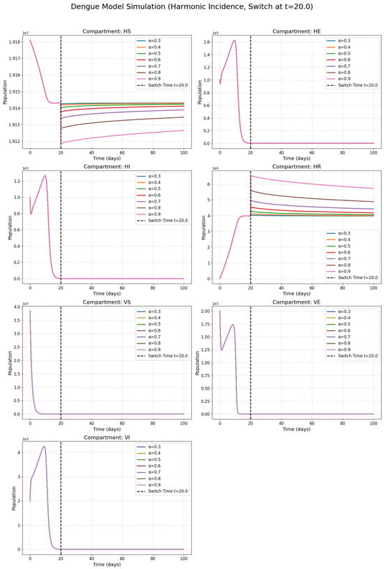
Figure 2.
Numerical solutions of susceptible individuals, exposed individuals, infected individuals, recovered individuals, susceptible mosquitoes, exposed mosquitoes, and infected mosquitoes at various fractional orders with the harmonic incidence rate.
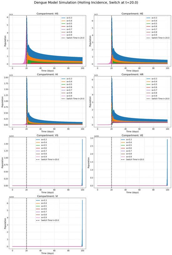
Figure 3.
Numerical solutions of susceptible individuals, exposed individuals, infected individuals, recovered individuals, susceptible mosquitoes, exposed mosquitoes, and infected mosquitoes at various fractional orders with The Holling incidence rate.
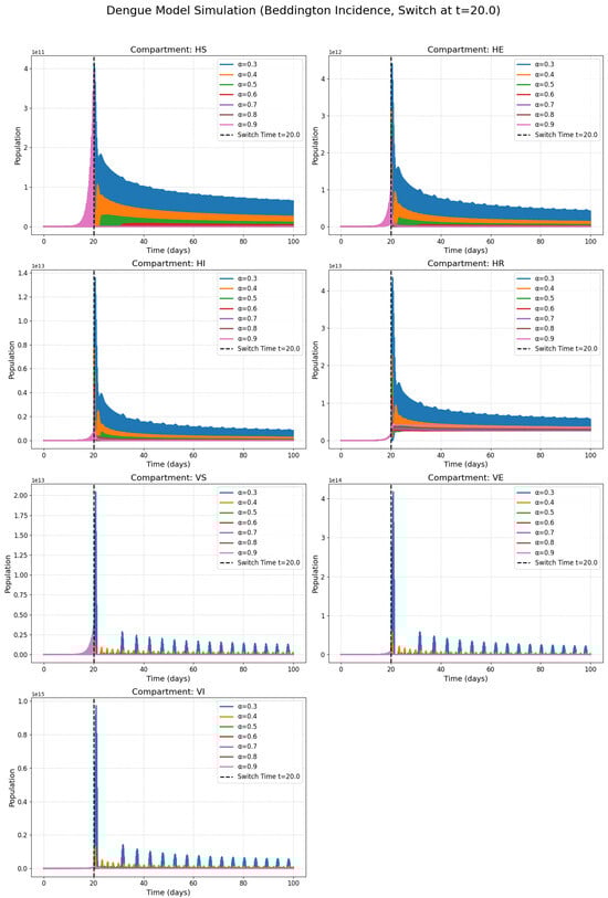
Figure 4.
Numerical solutions of susceptible individuals, exposed individuals, infected individuals, recovered individuals, susceptible mosquitoes, exposed mosquitoes, and infected mosquitoes at various fractional orders with the Beddington incidence rate.
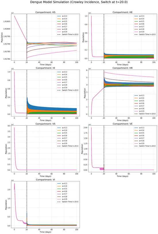
Figure 5.
Numerical solutions of susceptible individuals, exposed individuals, infected individuals, recovered individuals, susceptible mosquitoes, exposed mosquitoes, and infected mosquitoes at various fractional orders with the Crowley incidence rate.
Figure 2, Figure 3, Figure 4 and Figure 5 present the numerical simulations for each of the four incidence rates. Qualitatively, the dynamics of the infected compartments in each model exhibit a pattern consistent with typical single-strain epidemic outbreaks: an initial exponential rise in cases, followed by a peak and a subsequent decline as the susceptible population is depleted. The key differences, as we will discuss, lie in the magnitude and timing of these peaks and the long-term equilibrium behavior, which are directly influenced by the choice of incidence function and the fractional order.
Figure 2, Figure 3 and Figure 4 collectively serve as the visual output of the numerical simulations performed in this study. Each figure is dedicated to illustrating the dynamics of the dengue transmission model under one specific non-linear incidence rate formulation, all within the framework of the piecewise modified Atangana–Baleanu–Caputo (PMABC) fractional derivative. Figure 2 (Harmonic Mean) simulates the model using the Harmonic Mean incidence rate. It displays the time evolution of all seven compartments (susceptible humans , exposed humans , infectious humans , recovered humans , susceptible mosquitoes , exposed mosquitoes , infectious mosquitoes ). The curves within each subplot represent simulations performed with varying fractional orders in the plots. The plots mark the “Switch Time ”, indicating the point where the model transitions from classical to fractional dynamics as defined by the PMABC operator. The dynamics shown reflect the specific transmission behavior assumed by the Harmonic Mean rate. Figure 3 (Holling Type II), analogous to Figure 3, presents the simulation results when the Holling Type II (saturation) incidence rate is employed. Again, the temporal dynamics of all compartments are shown for various fractional orders under the PMABC framework with the same switch time. The expected visual difference compared to Figure 2 would stem from the saturation effect inherent in the Holling II function, potentially leading to different peak sizes or stabilization levels, especially under high infection pressure. Figure 4 (Beddington–DeAngelis) corresponds to the simulations using the Beddington–DeAngelis (B-D) incidence rate. This rate incorporates effects related to both susceptible and infectious populations (e.g., preventive measures by susceptibles and interference among infectious individuals/vectors). The resulting curves, plotted for different fractional orders within the PMABC structure, would visually differ from Figure 2 and Figure 3 due to these more complex interaction assumptions. Finally, Figure 5 (Crowley–Martin) shows the model dynamics when the Crowley–Martin incidence rate is used, which introduces mutual interference terms for both interacting populations. As with the previous figures, it illustrates the compartment evolutions over time for various fractional orders “s” under the piecewise operator. The specific form of this rate would lead to distinct dynamic patterns compared to the other three scenarios. The critical value of presenting these four figures side-by-side lies in their comparative potential. By keeping the underlying model structure (compartments, parameters, PMABC framework, and switch time) constant and only changing the incidence rate function, these figures are designed to visually highlight how significantly this single structural choice—representing the assumed mechanism of infection transmission—can alter the predicted course of the dengue epidemic. A visual comparison of the simulations reveals critical differences in predicted outbreak dynamics. The Holling Type II model (Figure 3), for instance, exhibits a saturation effect that results in a lower but more prolonged epidemic peak compared to the sharp, intense outbreak predicted by the Harmonic Mean model (Figure 2). Furthermore, the Beddington–DeAngelis and Crowley–Martin models (Figure 4 and Figure 5), which account for interference, predict a more rapid decline post-peak, suggesting that behavioral changes can significantly shorten an outbreak’s duration. Differences in peak infection levels, the timing of peaks, the rate of decline, and the final equilibrium states across Figure 2, Figure 3, Figure 4 and Figure 5 would underscore the importance of selecting an appropriate incidence rate based on biological realism and data fitting. Furthermore, observing how the fractional order modifies the dynamics within each figure demonstrates the added layer of complexity and potential realism offered by the fractional calculus approach.
8. Conclusions
We have developed and comprehensively analyzed a dengue fever transmission model utilizing the novel piecewise modified Atangana–Baleanu–Caputo (PMABC) fractional derivative framework. The primary contribution involved a systematic comparative investigation of the model’s dynamics under four distinct and sophisticated non-linear incidence functions: Harmonic Mean, Holling Type II, Beddington–DeAngelis, and Crowley–Martin. This specific PMABC operator was employed to capture potential temporal heterogeneity in transmission dynamics, allowing for an initial classical phase followed by a fractional phase potentially reflecting memory effects or accumulated impacts over the course of an epidemic. We have established the model’s well-posedness (positivity and boundedness of solutions), determined the basic reproduction number () for each incidence rate variant using the next-generation matrix method, and assessed the stability of the disease-free equilibrium based on . Furthermore, a comparative sensitivity analysis quantified how key epidemiological parameters influence across the four different model structures. These analytical findings were complemented by numerical simulations, using a tailored scheme derived from the fundamental definition of the PMABC operator, which visualized the distinct dynamic behaviors resulting from each incidence rate choice under varying fractional orders. The central finding of this study underscores that the selection of the non-linear incidence rate function critically impacts key epidemiological predictions, even when embedded within the same sophisticated PMABC fractional framework. While the Beddington–DeAngelis and Crowley–Martin models yielded identical expressions and similar sensitivity profiles at the DFE within this framework, the underlying non-linear dynamics, particularly away from the DFE suggested by simulations, can differ. The Harmonic Mean and Holling Type II models also presented unique characteristics regarding structure and parameter sensitivities (e.g., differing sensitivities to mosquito recruitment and mortality ). This comparative analysis demonstrates the necessity of carefully considering the biological assumptions underpinning the choice of incidence rate, as it significantly alters model outcomes concerning transmission thresholds, parameter importance, and overall system dynamics. The study also highlights the utility of the PMABC operator in providing a flexible structure to model potential crossover behavior in epidemic dynamics, offering a more nuanced approach than traditional integer-order or standard fractional models alone. The findings provide valuable insights for model selection in future dengue research and for the assessment of potential intervention strategies, emphasizing that predictions and inferred control targets can be highly sensitive to the chosen mathematical representation of the transmission mechanism. Despite the comprehensive nature of this comparative analysis, we acknowledge several limitations. First, this study is primarily theoretical; the parameter values were adopted from existing literature and not fitted to a specific epidemiological dataset. Real-world applications would require rigorous parameter estimation and model validation against dengue incidence data. Second, the model assumes homogeneous mixing, neglecting heterogeneities such as age structure, spatial distribution, and variations in socioeconomic conditions, which can significantly impact transmission. Finally, our model does not account for other important biological factors, such as different dengue serotypes, co-infections, or the influence of climate variables on mosquito populations.
From a public health perspective, our findings have direct policy implications. The consistently high sensitivity of to the vector mortality rate () across the more complex models (Holling II, B-D, Crowley–Martin) provides robust theoretical support for prioritizing vector control strategies, such as insecticide spraying and larval source reduction. Furthermore, the explicit inclusion of behavioral parameters in the Beddington–DeAngelis and Crowley–Martin models demonstrates that public health campaigns aimed at reducing human–vector contact can significantly lower the transmission potential. Our framework provides a tool for quantitatively estimating the potential effectiveness of such combined interventions.
In conclusion, this work not only provides a robust comparison of common incidence functions but also demonstrates the power of the PMABC fractional framework to advance the modeling of complex, evolving disease dynamics, offering a significant improvement in realism over models that assume static dynamics, whether integer-order or constant-order fractional.
Future work should aim to address the following points.
- Model Calibration and Validation: Applying the framework to real-world dengue incidence data from a specific region to estimate parameters and validate predictions.
- Multi-Strain Dynamics: Extending the model to include the co-circulation of multiple dengue serotypes, which is crucial for understanding antibody-dependent enhancement.
- Spatial Heterogeneity: Incorporating spatial dynamics to model transmission between different geographical areas (e.g., urban vs. rural).
- Stochastic Formulation: Developing a stochastic version of the model to account for random fluctuations and generate prediction confidence intervals.
- Sensitivity to : Performing a rigorous sensitivity analysis of the crossover point to quantify the impact of intervention timing.
Author Contributions
Conceptualization, F.H.D. and M.A. (Mohammed Almalahi); methodology, M.A. (Mohammed Almalahi); funding acquisition, A.A.Q.; formal analysis, M.A. (Mohammed Almalahi); investigation, M.A. (Mohammed Adel) and A.M.A.E.-L.; writing—original draft preparation, M.A. (Mohammed Almalahi); writing—review and editing, M.A. (Mohammed Adel), K.A., A.A.Q. and E.I.H.; visualization, F.H.D., A.M.A.E.-L. and E.I.H.; supervision, M.A. (Mohammed Almalahi) and K.A.; project administration, K.A. All authors have read and agreed to the published version of the manuscript.
Funding
This work was supported and funded by the Deanship of Scientific Research at Imam Mohammad Ibn Saud Islamic University (IMSIU) (grant number IMSIU-DDRSP2502).
Data Availability Statement
All data used in this work are contained within the article.
Conflicts of Interest
The authors declare no conflicts of interest.
References
- World Health Organization. Dengue–Guidelines for Diagnosis, Treatment, Prevention and Control, new ed.; WHO: Geneva, Switzerland, 2009; Available online: https://www.who.int/publications/i/item/9789241547871 (accessed on 2 February 2012).
- Loyinmi, A.C.; Gbodogbe, S.O. Mathematical modeling and control strategies for Nipah virus transmission incorporating bat-to-pig-to-human pathway. EDUCATUM J. Sci. Math. Technol. 2024, 11, 54–80. [Google Scholar] [CrossRef]
- Madueme, P.G.; Chirove, F. A systematic review of mathematical models of Lassa fever. Math. Biosci. 2024, 374, 109227. [Google Scholar] [CrossRef]
- Naaly, B.Z.; Marijani, T.; Isdory, A.; Ndendya, J.Z. Mathematical modeling of the effects of vector control, treatment and mass awareness on the transmission dynamics of dengue fever. Comput. Methods Programs Biomed. Update 2024, 6, 100159. [Google Scholar] [CrossRef]
- Malik, K.; Althobaiti, S. Impact of the infected population and nonlinear incidence rate on the dynamics of the SIR model. Adv. Contin. Discret. Model. 2025, 2025, 21. [Google Scholar] [CrossRef]
- Wang, D.; Zhao, Y.; Luo, J.; Leng, H. Simplicial SIRS epidemic models with nonlinear incidence rates. Chaos Interdiscip. J. Nonlinear Sci. 2021, 31, 053112. [Google Scholar] [CrossRef]
- Holling, C.S. Some characteristics of simple types of predation and parasitism. Can. Entomol. 1959, 91, 385–398. [Google Scholar] [CrossRef]
- Cosner, C.; DeAngelis, D.L.; Ault, J.S.; Olson, D.B. Effects of spatial grouping on the functional response of predators. Theor. Popul. Biol. 1999, 56, 65–75. [Google Scholar] [CrossRef]
- Aldwoah, K.A.; Almalahi, M.A.; Shah, K.; Awadalla, M.; Egami, R.H. Dynamics analysis of dengue fever model with harmonic mean type under fractal-fractional derivative. AIMS Math. 2024, 9, 13894–13926. [Google Scholar] [CrossRef]
- Riaz, M.; Alqarni, F.A.; Aldwoah, K.; Birkea, F.M.O.; Hleili, M. Analyzing a Dynamical System with Harmonic Mean Incidence Rate Using Volterra–Lyapunov Matrices and Fractal-Fractional Operators. Fractal Fract. 2024, 8, 321. [Google Scholar] [CrossRef]
- Mohsen, A.A.; Al-Husseiny, H.F.; Hattaf, K. The awareness effect of the dynamical behavior of SIS epidemic model with Crowley-Martin incidence rate and holling type III treatment function. Int. J. Nonlinear Anal. Appl. 2021, 12, 1083–1097. [Google Scholar]
- Mahato, P.; Mahato, S.K.; Das, S. A stochastic epidemic model with Crowley–Martin incidence rate and Holling type III treatment. Decis. Anal. J. 2024, 10, 100391. [Google Scholar] [CrossRef]
- Velten, K.; Schmidt, D.M.; Kahlen, K. Mathematical Modeling and Simulation: Introduction for Scientists and Engineers; John Wiley & Sons: Hoboken, NJ, USA, 2024. [Google Scholar]
- Jan, R.; Ahmad, I.; Ahmad, H.; Vrinceanu, N.; Hasegan, A.G. Insights into dengue transmission modeling: Index of memory, carriers, and vaccination dynamics explored via non-integer derivative. AIMS Bioeng. 2024, 11, 44–65. [Google Scholar] [CrossRef]
- Kumar, A.; Nilam. Dynamical model of epidemic along with time delay; Holling type II incidence rate and Monod–Haldane type treatment rate. Differ. Equ. Dyn. Syst. 2019, 27, 299–312. [Google Scholar] [CrossRef]
- Riaz, M.; Khan, Z.A.; Ahmad, S.; Ateya, A.A. Fractional-Order Dynamics in Epidemic Disease Modeling with Advanced Perspectives of Fractional Calculus. Fractal Fract. 2024, 8, 291. [Google Scholar] [CrossRef]
- Wang, W.; Liu, T.; Fan, X. Mathematical modelling of cholera disease with seasonality and human behavior change. Discret. Contin. Dyn. Syst. B 2024, 29, 3531–3556. [Google Scholar] [CrossRef]
- Atangana, A.; Baleanu, D. New fractional derivatives with nonlocal and non-singular kernel: Theory and application to heat transfer model. Therm. Sci. 2016, 20, 763. [Google Scholar] [CrossRef]
- Atangana, A.; Araz, S.I. New concept in calculus: Piecewise differential and integral operators. Chaos Solitons Fractals 2021, 145, 110638. [Google Scholar] [CrossRef]
- Madani, Y.A.; Almalahi, M.A.; Osman, O.; Muflh, B.; Aldwoah, K.; Mohamed, K.S.; Eljaneid, N. Analysis of an Acute Diarrhea Piecewise Modified ABC Fractional Model: Optimal Control, Stability and Simulation. Fractal Fract. 2025, 9, 68. [Google Scholar] [CrossRef]
- Xu, C.; Liu, Z.; Pang, Y.; Akgul, A.; Baleanu, D. Dynamics of HIV-TB coinfection model using classical and Caputo piecewise operator: A dynamic approach with real data from South-East Asia, European and American regions. Chaos Solitons Fractals 2022, 165, 112879. [Google Scholar] [CrossRef]
- Al-Refai, M.; Baleanu, D. On an extension of the operator with Mittag-Leffler kernel. Fractals 2022, 30, 2240129. [Google Scholar] [CrossRef]
- Ahmad, S.; Yassen, M.F.; Alam, M.M.; Alkhati, S.; Jarad, F.; Riaz, M.B. A numerical study of dengue internal transmission model with fractional piecewise derivative. Results Phys. 2022, 39, 105798. [Google Scholar] [CrossRef]
- Aldwoah, K.A.; Almalahi, M.A.; Shah, K. Theoretical and numerical simulations on the hepatitis B virus model through a piecewise fractional order. Fractal Fract. 2023, 7, 844. [Google Scholar] [CrossRef]
- Alazman, I.; Alkahtani, B.S.T. Investigation of Novel Piecewise Fractional Mathematical Model for COVID-19. Fractal Fract. 2022, 6, 661. [Google Scholar] [CrossRef]
- Saber, H.; Almalahi, M.A.; Albala, H.; Aldwoah, K.; Alsulami, A.; Shah, K.; Moumen, A. Investigating a Nonlinear Fractional Evolution Control Model Using W-Piecewise Hybrid Derivatives: An Application of a Breast Cancer Model. Fractal Fract. 2024, 8, 735. [Google Scholar] [CrossRef]
- Khan, H.; Alzabut, J.; Gómez-Aguilar, J.F.; Alkhazan, A. Essential criteria for existence of solution of a modified-ABC fractional order smoking model. Ain Shams Eng. J. 2024, 15, 102646. [Google Scholar] [CrossRef]
- Meetei, M.Z.; Zafar, S.; Zaagan, A.A.; Mahnashi, A.M.; Idrees, M. Dengue transmission dynamics: A fractional-order approach with compartmental modeling. Fractal Fract. 2024, 8, 207. [Google Scholar] [CrossRef]
- Abboubakar, H.; Gouroudja, S.A.B.; Richard, Y.; Jan, R. Fractional dynamics of a two-strain dengue model with co-infections and saturated incidences. Int. J. Biomath. 2024. [Google Scholar] [CrossRef]
- Yang, J.; Tang, S. Holling type II predator–prey model with nonlinear pulse as state-dependent feedback control. J. Comput. Appl. Math. 2016, 291, 225–241. [Google Scholar] [CrossRef]
- Huang, G.; Takeuchi, Y. Global analysis on delay epidemiological dynamic models with nonlinear incidence. J. Math. Biol. 2011, 63, 125–139. [Google Scholar] [CrossRef]
- Upadhyay, R.K.; Pal, A.K.; Kumari, S.; Roy, P. Dynamics of an SEIR epidemic model with nonlinear incidence and treatment rates. Nonlinear Dyn. 2019, 96, 2351–2368. [Google Scholar] [CrossRef]
- Zhang, S.; Tan, D.; Chen, L. Dynamic complexities of a food chain model with impulsive perturbations and Beddington–DeAngelis functional response. Chaos Solitons Fractals 2006, 27, 768–777. [Google Scholar] [CrossRef]
- Singh, H. Analysis for fractional dynamics of Ebola virus model. Chaos Solitons Fractals 2020, 138, 109992. [Google Scholar] [CrossRef]
- Singh, H.; Srivastava, H.M.; Hammouch, Z.; Nisar, K.S. Numerical simulation and stability analysis for the fractional-order dynamics of COVID-19. Results Phys. 2021, 20, 103722. [Google Scholar] [CrossRef] [PubMed]
- Singh, H.; Baleanu, D.; Singh, J.; Dutta, H. Computational study of fractional order smoking model. Chaos Solitons Fractals 2021, 142, 110440. [Google Scholar] [CrossRef]
- Pandey, H.R.; Phaijoo, G.R. Analysis of dengue infection transmission dynamics in Nepal using fractional order mathematical modeling. Chaos Solitons Fractals X 2023, 11, 100098. [Google Scholar] [CrossRef]
- Crowley, P.H.; Martin, E.K. Functional responses and interference within and between year classes of a dragonfly population. J. N. Am. Benthol. Soc. 1989, 8, 211–221. [Google Scholar] [CrossRef]
- Khan, H.; Alzabut, J.; Gómez-Aguilar, J.F.; Agarwal, P. Piecewise mABC fractional derivative with an application. AIMS Math. 2023, 8, 24345–24366. [Google Scholar] [CrossRef]
- Diethelm, K.; Ford, N.J. The Analysis of Fractional Differential Equations; Lecture Notes in Mathematics; Springer: Berlin/Heidelberg, Germany, 2010; Volume 2004. [Google Scholar]
- van den Driessche, P.; Watmough, J. Reproduction numbers and sub-threshold endemic equilibria for compartmental models of disease transmission. Math. Biosci. 2002, 180, 29–48. [Google Scholar] [CrossRef]
- Andraud, M.; Hens, N.; Marais, C.; Beutels, P. Dynamic epidemiological models for dengue transmission: A systematic review of structural approaches. PLoS ONE 2012, 7, e49085. [Google Scholar] [CrossRef]
- Ogunlade, S.T.; Meehan, M.T.; Adekunle, A.I.; McBryde, E.S. A systematic review of mathematical models of dengue transmission and vector control: 2010–2020. Viruses 2023, 15, 254. [Google Scholar] [CrossRef]
- Vaidya, N.K.; Wang, F.B. Persistence of mosquito vector and dengue: Impact of seasonal and diurnal temperature variations. Discret. Contin. Dyn. Syst. 2022, 27, 393–420. [Google Scholar] [CrossRef]
- Bonyah, E.; Sagoe, A.K.; Kumar, D.; Deniz, S. Fractional optimal control dynamics of coronavirus model with Mittag–Leffler law. Ecol. Complex. 2021, 45, 100880. [Google Scholar] [CrossRef]
Disclaimer/Publisher’s Note: The statements, opinions and data contained in all publications are solely those of the individual author(s) and contributor(s) and not of MDPI and/or the editor(s). MDPI and/or the editor(s) disclaim responsibility for any injury to people or property resulting from any ideas, methods, instructions or products referred to in the content. |
© 2025 by the authors. Licensee MDPI, Basel, Switzerland. This article is an open access article distributed under the terms and conditions of the Creative Commons Attribution (CC BY) license (https://creativecommons.org/licenses/by/4.0/).