Article

Granular Fuzzy Fractional Continuous-Time Linear Systems: Roesser and Fornasini–Marchesini Models

1
Department of Mathematics, Lahore Garrison University, Lahore 54000, Pakistan
2
Institute of Mathematics, University of the Punjab, New Campus, Lahore 54590, Pakistan
3
Department of Mathematics, King Abdulaziz University, P.O Box 80203, Jeddah 21589, Saudi Arabia
*
Author to whom correspondence should be addressed.
Fractal Fract. 2025, 9(7), 398; https://doi.org/10.3390/fractalfract9070398
Submission received: 15 May 2025 / Revised: 4 June 2025 / Accepted: 16 June 2025 / Published: 20 June 2025
(This article belongs to the Special Issue Fractional Mathematical Modelling: Theory, Methods and Applications)

Abstract

In this article, we introduce and investigate two classes of fuzzy fractional two-dimensional continuous-time (FFTDCT) linear systems to deal with uncertainty and fuzziness in system parameters. First, we analyze FFTDCT linear systems based on the Roesser model, incorporating fuzzy parameters into the state-space equations. The potential solution of the fuzzy fractional system is obtained using a two-dimensional granular Laplace transform approach. Second, we examine FFTDCT linear systems described by the second Fornasini–Marchesini (FM) model, where the state-space equations involve two-dimensional and one-dimensional partial fractional-order granular Caputo derivatives. We determine the fuzzy solution for this model by applying the two-dimensional granular Laplace transform. To enhance the validity of the proposed approaches, real-world applications, including signal processing systems and wireless sensor network data fusion, are solved to support the theoretical framework and demonstrate the impact of uncertainty on the system’s behavior.

1. Introduction

All real-world phenomena are naturally affected by uncertainty. Developing a model, solving the problem, and analyzing the results encountered are essential tasks within the domain of fuzziness. Generally, differential equations (DEs) are commonly involved in various scientific and engineering domains [1]. These DEs typically rely on complex environments, and such complexities can be handled more precisely using fractional-order derivatives. In contrast, the model’s parameters, variables, and initial or boundary conditions are assumed to be crisp for computational simplicity. Errors that arise from observations, measurements, or experiments can result in vague or incomplete descriptions of these parameters and variables. One can employ a stochastic, statistical, or fuzzy approach to deal with such uncertainty. Stochastic and statistical methods address the uncertainty due to inherent randomness in processes. Fuzzy set theory offers a framework for managing vagueness and imprecision that result from incomplete information regarding the variables and parameters of a model.
Fuzzy differential equations (FDEs) have become a valuable tool for modeling natural phenomena and are characterized by uncertainty, attracting considerable attention from researchers. The concept of FDEs was first introduced by Dubois and Prade in 1982 [2]. Many researchers have worked on FDEs by examining their existence and uniqueness (E&U), proposing novel approaches, and determining the behavior to deepen the comprehension of the models [3,4,5]. The solution was derived using the fuzzy Laplace transform technique [3,6,7].
The fuzzy derivatives obtained from fuzzy standard interval arithmetic (FSIA) possess some limitations. Some of them are highlighted below: (i) The solution of FDEs under fuzzy derivatives leads to CPLV [8]. Furthermore, all real-world phenomena are governed by physical laws, and these problems are often described using FDEs. However, FDEs can admit multiple fuzzy solutions, and not all of them may accurately reflect the true behavior of the physical system. Inaccurate or inappropriate solutions can lead to predictions that contradict the underlying physical principles. (ii) The fuzzy derivatives within the FSIA framework are valid only if the H-difference exists. The existence of fuzzy derivatives is restricted if the corresponding differences do not exist [9]. (iii) The n-dimensional FDEs under FSIA are transformed into a 2 n classical system. This transformation imposes a constraint that complicates the comprehension and analysis of FDEs. (iv) FDEs under fuzzy derivatives with FSIA lead to different solutions. This phenomenon is commonly referred to as the UBM phenomenon. (v) The FDEs using FSIA frequently yield multiple or infinitely many solutions, complicating the interpretation of the results [10]. Mazandarani et al. [9] introduced the novel concept of differentiability, commonly called granular differentiability ( g r -derivative), to explore the FDEs from a new perspective. This approach handles the fuzziness of FDEs by applying the fuzzy interval arithmetic based on the relative distance measure (RDM). The core innovation behind this approach is to characterize fuzzy numbers through their horizontal membership function (HMF) and to formulate the corresponding operations within this framework. This derivative is introduced to overcome the limitations of fuzzy derivatives using FSIA. FDEs based on the g r -derivative enable us to determine a unique solution to the problem. Granular differentiability (GRD) has the following main advantages when investigating FDEs: FDEs under GRD have a simple and effective solution. In FDEs involving GRD, the solution’s support across the domain does not need to be intrinsically monotonic. The doubling property, multiplicity, and UBM phenomena constraints are successfully addressed and eliminated in the solutions of FDEs using GRD.

Motivation and Contribution

The modeling of complex multi-dimensional dynamical processes with memory and hereditary properties relies heavily on fractional two-dimensional continuous-time (FTDCT) linear systems. These systems are essential for studying real-world phenomena, including distributed parameter systems, thermal systems, and image processing. One effective tool for examining and managing such systems is the extension of the Roesser model to the fractional calculus. Roesser [11] introduced the most significant state-space models for two-dimensional linear systems (TDLSs). For the study of multi-dimensional systems, this model is essential. To evaluate two-dimensional linear systems (TDLSs), they offer a framework that separates the dynamics into vertical and horizontal components. Alternative state-space models for TDLSs were proposed by Fornasini and Marchesini [12] and are widely used for the study and control of multi-dimensional systems. This work extends the Roesser model and provides additional tools for understanding two-dimensional (2D) systems, particularly in the context of iterative processes and signal processing. The state-space model for TDLSs introduced by Kurek [13] is especially helpful for applications involving image processing and control systems. Kurek’s approach provides a consistent framework for TDLS modeling. This model is beneficial for analyzing systems with closely related spatial dimensions, such as image filtering and thermal processes. Bose [14] examined the fundamental ideas and revelations of TDLS theory. His work mainly concentrated on signal processing applications, system realization, and stability analysis. This work laid the groundwork for understanding the structural and behavioral characteristics of TDLSs. Kaczorek [15] studied TDLSs, focusing on their mathematical formulation and solution methods. He investigated the positive systems based on the ideas previously introduced in the literature. Galkowski [16] contributed theoretically by developing the state-space realizations of TDLSs and extending them into higher-dimensional systems. Farina and Rinaldi [17] studied positive linear systems with their applications. They also extended their work in the broader context of the TDLS. Oldham and Spanier [18] presented the basic concepts, definitions, and characteristics of fractional calculus, which are essential for future studies. Miller and Ross [19] explored fractional differential equations, emphasizing their applications across various fields by establishing connections between abstract mathematics and real-world problem-solving. Podlubny [20] discussed fractional differential equations and demonstrated their importance in simulating complex systems in control theory and engineering. Kaczorek [21] introduced the concept of fractional-order discrete TDLSs, laying the groundwork for further research into fractional-order dynamics. Rogowski [22] developed a general response formula for solving the FTDCT linear system of the Roesser structure with its applications. Kaczorek and Rogowski [23] studied the descriptor case of continuous fractional-order TDLSs. Their work broadened the applicability and understanding of fractional systems in multi-dimensional contexts. Rogowski [24] studied the behavior of fractional-order TDLSs described by the Roesser type. Idczak et al. [25] examined the solution of an FTDCT linear system of the first FM type, incorporating Riemann–Liouville (RL) fractional-order partial derivatives. Their findings provided valuable insights into how such derivatives influence the dynamics and behavior of these systems. Rogowski [26] examined the FM model’s positive analysis for continuous fractional-order TDLSs. Using the Roesser model, Hu et al. [27] investigated the event-triggered control methods for continuous TDLSs. Reducing communication frequency and minimizing dependency on global information are the goals of this strategy. The stability of generalized nonlinear homogeneous systems in the presence of bounded disturbances was examined by Huang et al. [28]. The conditions under which these systems maintain their stability in the face of external perturbations were carefully studied in this work. Using the concept of bounded disturbances, Ma et al. [29] investigated the estimation of the reachable set for 2D switched nonlinear positive systems, taking time-varying delays and delayed impulsive effects into account. Using the Roesser framework, Dami and Benzaouia [30] presented a new kind of 2D fractional switched system. To use state feedback controllers to stabilize the system, the study also investigated sufficient conditions (SCs). Under the Roesser framework, Huang et al. [31] examined the finite-time stability (FTS) of 2D positive systems. The study employed a co-positive Lyapunov function to construct SCs to accomplish FTS in the system. In the framework of the Roesser model, Gao et al. [32] examined the SCs for the FTS and finite-time control (FTC) of 2D systems. To mitigate the effect of stable bounded disturbance inputs on TDLSs in the Roesser framework, Ahn et al. [33] introduced a linear matrix inequality (LME) condition. The analysis used discrete Jensen inequality (DJI) and diagonally dominant matrices (DDMs). Nemati and Mamehrashi [34] developed the numerical scheme for 2D fractional optimal control systems using Legendre polynomials, the Ritz approach, and the Laplace transform technique. They also analyzed the convergence with two illustrative examples.
Zhang et al. [35] analyzed the necessary SCs for the stability of the 2D fractional first FM model. They presented these conditions with respect to polynomials and LMEs using the Kronecker product. Zhu and Lu [36] discussed the robust stability of the second 2D FM continuous fractional-order model in the presence of interval uncertainties. They determined the LMI-based stability conditions using the nominal fractional-order model, which was presented in terms of stable root clustering sets. Zhang and Wang [37] formulated the concepts of finite-region stability and boundedness of the 2D fractional-order second FM model and then analyzed the transient behavior of such systems. Benyettou et al. [38] determined the solution procedure of conformable fractional TDLSs by applying the Laplace and Sumudu transform techniques. Benyettou et al. [39] formulated the solution to the minimum energy control problem for fractional TDLSs described by the first FM model. Yan et al. [40] developed the state-space formulation for the 2D frequency transformation in the second FM model, which enables a more flexible tool for 2D zero-phase filters to prevent image distortions. Li and Hou [41] introduced the parametric controller method for TDLSs using polynomial discriminant systems and the Hurwitz theorem. The main contributions of the proposed work in this area are summarized as follows:
1.
Two classes of FFTDCT linear systems are introduced and investigated to address uncertainty and fuzziness in system parameters.
2.
The fuzzy solution of FFTDCT linear systems based on the Roesser model and the second FM model is obtained under one-dimensional 2D partial fractional granular Caputo derivatives.
3.
The potential solution of the proposed model is determined using the 2D granular Laplace transform.
4.
Real-world applications, including signal processing systems and wireless sensor network data fusion, are solved using the proposed technique.
The rest of the article is organized as follows: some fundamental concepts of the granular representation of the fuzzy number, 2D granular fractional integral (GFI), 2D granular Caputo fractional derivatives (GCFDs), and 2D granular Laplace transform are presented in Section 2. The fuzzy solution of the granular FFTDCT Roesser model using the granular 2D fuzzy Laplace transform is determined in Section 3. The fuzzy solution of the granular FFTDCT described by the second FM model is extracted in Section 4. The applications of the FFTDCT linear system described by Roesser and FM’s second model are discussed in Section 5. Section 6 outlines the conclusion of the article.

2. Fuzzy Preliminaries

This section introduces the basic concepts of fuzzy analysis, including granular representations and their associated operations. Subsequently, we define the two-dimensional Riemann–Liouville (2DRL) fractional integral and the fractional derivative in Caputo sense. Moreover, we extend these concepts with the granular counterparts through the two-dimensional GFI and two-dimensional GCFD. The section further develops the theoretical framework by presenting the 2D granular Laplace transform and examining its key properties.
A fuzzy set m [42] m : [ a , b ] R [ 0 , 1 ] is referred to as the fuzzy number (FN) if it adheres to the following properties: normal, upper semicontinuity, convex and has compact support. Let Ξ R denote the class of all FNs on R . The ϑ -cut of m is denoted by [ m ] ϑ and is defined by [ m ] ϑ = [ m ϑ , m ϑ + ] , for all 0 ϑ 1 .
Definition 1
([9]). Let m be an FN; the granular representation of m is defined as m gr : [ 0 , 1 ] × [ 0 , 1 ] [ a , b ] , where ( ϑ , π ) m gr ( ϑ , π ) = m ϑ + ( m ϑ + m ϑ ) π . Here, “gr” denotes the granular representation of m over the interval x [ a , b ] , with ϑ [ 0 , 1 ] and π [ 0 , 1 ] . The HMF of FN m is represented by H ( m ) and is defined by H ( m ) m gr ( ϑ , π ) .
We now provide Table 1, which includes various commonly used notations.
Definition 2
([9]). The ϑ-cut of m Ξ R can be represented by the following formula
H 1 ( m g r ( ϑ , π ) ) : = [ m ] ϑ : = inf η ϑ min π m g r ( η , π ) , sup η ϑ max π m g r ( η , π ) .
Definition 3
([9]). The arithmetic operations of two FNs, m 1 and m 2 , with their HMFs, H ( m 1 ) and H ( m 2 ) , respectively, are defined by
H ( m 1 m 2 ) = H ( m 1 ) H ( m 2 ) ,
whereanddenote the arithmetic operations on Ξ R and R , respectively, such as addition, subtraction, multiplication, or division.
Definition 4
([9]). Suppose ϰ : [ a , b ] R Ξ R is a fuzzy function that includes m 1 , m 2 , m 3 , , m n FNs. The HMF of ϰ ( z ) , represented by H ( ϰ ( z ) ) ϰ gr ( z , ϑ , π ) , is described by the given relation
ϰ gr : [ a , b ] × [ 0 , 1 ] × [ 0 , 1 ] n R , where ϑ [ 0 , 1 ] and π ( π m 1 , π m 2 , , π m n ) .
Definition 5
([43]). Let m 1 , m 2 , m 3 Ξ R , and λ be a real number. Then, the below claims hold:
(i).
ρ gr ( m 1 + m 3 , m 2 + m 3 ) = ρ gr ( m 1 , m 2 ) .
(ii).
ρ gr ( λ m 1 , λ m 2 ) = | λ | ρ gr ( m 1 , m 2 ) .
(iii).
ρ gr ( m 1 gr m 2 , 0 ^ ) = ρ gr ( m 1 , m 2 ) .

2.1. Fuzzy Fractional Calculus

Definition 6
([9]). Let ϰ : ( a , b ) R Ξ R be an FVF. The function ϰ is said to be GRD at z ( a , b ) if there exists ϰ gr ( z ) Ξ R such that the following limit
ϰ gr ( z ) = lim ϵ 0 ϰ ( z + ϵ ) gr ϰ ( z ) ϵ ,
exists.
Definition 7.
The fractional integral (FI) of ϰ L 1 ( [ a , b ] , R ) of order α > 0 , denoted by I a + α , is defined by
I a + α ϰ ( z ) = 1 Γ ( α ) a z ( z τ ) α 1 ϰ ( τ ) d τ .
Definition 8
([20,44]). The FI of order α > 0 of ϰ ( z 1 , z 2 ) regarding the variable z 1 is defined by
I z 1 α ϰ ( z 1 , z 2 ) = 1 Γ ( α ) a z 1 ( z 1 τ ) α 1 ϰ ( τ , z 2 ) d τ .
Similarly, we can define the RL fractional integral of a 2D continuous function ϰ ( z 1 , z 2 ) regarding z 2 .
Now, we define the following Definition 9 for the 2DRL fractional integral regarding the variables z 1 and z 2 based on Definition 8, as follows:
Definition 9
([20,44]).  The two-dimensional RL fractional integral of order α i of a continuous function ϰ ( z 1 , z 2 ) regarding variable z i ( i = 1 , 2 ) is given by the formula
I z i α i ϰ ( z 1 , z 2 ) = 1 Γ ( α i ) a z i ( z i τ ) α i 1 ϰ ( τ ) d τ ,
where
ϰ ( τ ) = ϰ ( τ , z 2 ) f o r i = 1 , ϰ ( z 1 , τ ) f o r i = 2 .
Definition 10.
The CFD of order α > 0 , denoted by D a + α C , of a function ϰ C 1 ( [ a , b ] , R ) , is defined by
D a + α C ϰ ( z ) : = 1 Γ ( n α ) a z ( z τ ) n α 1 ϰ ( n ) ( τ ) d τ ,
where n N , such that n 1 < α < n , and z [ a , b ] .
Definition 11
([22,23]). The CFD of order α > 0 of a 2D continuous function ϰ ( z 1 , z 2 ) regarding variable z 1 is given by
D a + α C ϰ ( z 1 , z 2 ) = 1 Γ ( n α ) a z 1 f ( n ) ( τ , z 2 ) ( z 1 τ ) α n + 1 d τ ,
where n 1 α < n . Similarly, we can define the aforementioned CFD of a 2D continuous function ϰ ( z 1 , z 2 ) regarding z 2 .
We now define the following Definition 12 for the two-dimensional Caputo fractional derivative (2DCFD) regarding the variables z 1 and z 2 based on Definition 11, as follows:
Definition 12
([22,23]). The 2DCFD of order α i > 0 of a continuous function ϰ ( z 1 , z 2 ) regarding variable z i   ( i = 1 , 2 ) is given by
D z i α i C ϰ ( z 1 , z 2 ) = 1 Γ ( n i α i ) a z i f ( n i ) ( τ ) ( z i τ ) α i n i + 1 d τ ,
where n i 1 α i < n i , and
f ( n i ) ( τ ) = n i τ n i ϰ ( τ , z 2 ) f o r i = 1 , n i τ n i ϰ ( z 1 , τ ) f o r i = 2 .
Based on Definition 9, we present the idea of the GFI of FVFs as follows:
Definition 13.
Let ϰ : [ a 1 , b 1 ] × [ a 2 , b 2 ] R 2 E R . The GFI of order α i ( 0 , 1 ] of FVF is defined by
I z i α i gr ϰ ( z 1 , z 2 ) = 1 Γ ( α i ) a t i ( t i τ ) α i 1 ϰ ( τ ) d τ ,
where ϰ ( τ ) is ϰ ( τ , z 2 ) for i = 1 and ϰ ( z 1 , τ ) for i = 2 , respectively.
Remark 1.
According to Definition 13, the HMF of granular fractional integral I z i α i gr ϰ ( z 1 , z 2 ) is defined by
H I z i α i gr ϰ ( z 1 , z 2 ) = 1 Γ ( α i ) a z i H ( z i τ ) α i 1 ϰ ( τ ) d τ , = 1 Γ ( α i ) a z i ( z i τ ) α i 1 H ϰ ( τ ) d τ , = I z i α i H ϰ ( τ ) .
Thus, H I z i α i gr ϰ ( z 1 , z 2 ) = I z i α i H ϰ ( τ ) , where ϰ ( τ ) is ϰ ( τ , z 2 ) for i = 1 and ϰ ( z 1 , τ ) for i = 2 , respectively.
Definition 14.
Let ϰ : [ a 1 , b 1 ] × [ a 2 , b 2 ] R 2 E R . The 2D GCFD of order α i ( 0 , 1 ] of the FVF ϰ ( z 1 , z 2 ) regarding variable z i ( i = 1 , 2 ) is defined by
D z i α i gr ϰ ( z 1 , z 2 ) = 1 Γ ( 1 α i ) a z i ϰ g r ( τ ) ( z i τ ) α i d τ ,
where ϰ g r ( τ ) is equal to τ ϰ g r ( τ , z 2 ) for i = 1 and τ ϰ g r ( z 1 , τ ) for i = 2 , respectively.
Remark 2.
Similar to Remark 1, we may also infer the following:
H D z i α i gr ϰ ( z 1 , z 2 ) = D z i α i C H ϰ ( z 1 , z 2 ) .

2.2. Granular 2D Laplace Transform for FVF

First, we review some fundamental concepts and terminology related to the Laplace transform of a 2D continuous function. Next, we present the granular 2D Laplace transform of FVF and HMF.
Definition 15
([20,23,45]). Let ϰ ( p , z 2 ) and ϰ ( z 1 , s ) denote the Laplace transforms of a 2D continuous function ϰ ( z 1 , z 2 ) regarding z 1 and z 2 , respectively. The following formulas define these transforms:
L z 1 [ ϰ ( z 1 , z 2 ) ] : = 0 ϰ ( z 1 , z 2 ) e p z 1 d z 1 , L z 2 [ ϰ ( z 1 , z 2 ) ] : = 0 ϰ ( z 1 , z 2 ) e s z 2 d z 2 .
Definition 16
([20,23,45]). Suppose ϰ ( z 1 , z 2 ) is the real-valued continuous function from [ 0 , ) × [ 0 , ) to R such that the 2D Laplace transform of ϰ ( z 1 , z 2 ) , denoted by χ ( p , s ) and defined by
χ ( p , s ) = L z 1 , z 2 ϰ ( z 1 , z 2 ) = L z 1 L z 2 ϰ ( z 1 , z 2 ) = L z 2 L z 1 ϰ ( z 1 , z 2 ) = 0 0 ϰ ( z 1 , z 2 ) e p z 1 s z 2 d z 1 d z 2 ,
for all p , s C for which the integral in Equation (9) converges.
Definition 17
([22,23]). The 2D Laplace transform of Definition 9 is given by
L z 1 , z 2 [ I z 1 α 1 ϰ ( z 1 , z 2 ) ] = p α 1 χ ( p , s ) and L z 1 , z 2 [ I z 2 α 2 ϰ ( z 1 , z 2 ) ] = s α 2 χ ( p , s ) .
Furthermore,
L z 1 t 1 α 1 1 Γ ( α 1 ) = p α 1 and L z 2 t 2 α 2 1 Γ ( α 2 ) = s α 2 ,
for α 1 > 0 and α 2 > 0 .
Theorem 1
([22,23]). The 2D Laplace transform of Definition 12 of the 2D function ϰ ( z 1 , z 2 ) regarding z 1 and z 2 is defined by
L z 1 , z 2 D α 1 0 + C ϰ ( z 1 , z 2 ) = p α 1 ϰ ( p , s ) k = 1 n 1 p α 1 k F ( k 1 ) ( 0 , s )
and
L z 1 , z 2 D α 2 0 + C ϰ ( z 1 , z 2 ) = s α 2 ϰ ( p , s ) l = 1 n 2 s α 2 l F ( l 1 ) ( p , 0 ) ,
respectively, where F ( k ) ( 0 , s ) = L z 2 k z 1 k ϰ ( z 1 , z 2 ) | z 1 = 0 and F ( l ) ( p , 0 ) = L z 1 l z 2 l ϰ ( z 1 , z 2 ) | z 2 = 0 for k , l Z + . Combining Equations (12) and (13), we get
L z 1 , z 2 D α 1 , α 2 0 + C ϰ ( z 1 , z 2 ) = p α 1 s α 2 ϰ ( p , s ) k = 1 n 1 l = 1 n 2 p α 1 k s α 2 l F ( k 1 , l 1 ) ( 0 , 0 ) p α 1 l = 1 n 2 s α 2 l F ( l 1 ) ( p , 0 ) s α 2 k = 1 n 1 p α 1 l F ( k 1 ) ( 0 , s ) ,
where F ( k , l ) ( 0 , 0 ) = k z 1 k l z 2 l ϰ ( z 1 , z 2 ) | z 1 = 0 , z 2 = 0 for k , l Z + .
Definition 18.
Suppose ϰ ( z 1 , z 2 ) is the continuous FVF such that e p z 1 s z 2 ϰ ( z 1 , z 2 ) is the improper fuzzy Riemann-integrable on [ 0 , ) × [ 0 , ) , and then L z 1 , z 2 ϰ ( z 1 , z 2 ) is called the granular 2D Laplace transform of ϰ ( z 1 , z 2 ) and is defined by
L z 1 , z 2 ϰ ( z 1 , z 2 ) = 0 0 e p z 1 s z 2 ϰ ( z 1 , z 2 ) d z 1 d z 2 ,
where p , s > 0 are integers.
Remark 3.
The HMF of Definition 18 is defined by
H L z 1 , z 2 ϰ ( z 1 , z 2 ) = 0 0 H e p z 1 s z 2 ϰ ( z 1 , z 2 ) d z 1 d z 2 , = 0 0 e p z 1 s z 2 H ϰ ( z 1 , z 2 ) d z 1 d z 2 , = L z 1 , z 2 H ϰ ( z 1 , z 2 ) .

3. Granular FFTDCT Linear Systems in the Roesser Framework

In this section, we derive the fuzzy solution of the granular FFTDCT Roesser model using the granular 2D fuzzy Laplace transform. To achieve this, we first define the granular FFTDCT linear system governed by the following state equations:
D α 1 0 + gr ϰ 1 ( z 1 , z 2 ) D α 2 0 + gr ϰ 2 ( z 1 , z 2 ) = A ϰ 1 ( z 1 , z 2 ) ϰ 2 ( z 1 , z 2 ) + B u ( z 1 , z 2 ) ,
y ( z 1 , z 2 ) = C ϰ 1 ( z 1 , z 2 ) ϰ 2 ( z 1 , z 2 ) + D u ( z 1 , z 2 ) ,
where A = [ a i j ] , B = [ b i ] for i , j = 1 , 2 , ϰ 1 ( z 1 , z 2 ) Ξ R n 1 , and ϰ 2 ( z 1 , z 2 ) Ξ R n 2 ( n = n 1 + n 2 ) are the fuzzy horizontal and fuzzy vertical state vectors, respectively. Moreover, u ( z 1 , z 2 ) Ξ R m and y ( z 1 , z 2 ) Ξ R p are the fuzzy inputs and output vectors of the system. Furthermore, A Ξ R n i × j , B Ξ R n i × m , C Ξ R p × n , and D Ξ R p × m are the fuzzy matrices. For simplicity, we consider the system (17) with fractional orders α 1 , α 2 ( 0 , 1 ) .
Note 1.
Let  Ξ R n × n  be the class of all fuzzy matrices of size n and  Ξ R n = Ξ R n × 1 . Moreover,  I n  is the identity matrix of size n.
Theorem 2.
The HMF of the fuzzy solution of system (17) with fractional orders 0 < α 1 < 1 , 0 < α 2 < 1 for arbitrary fuzzy input u ( z 1 , z 2 ) is given by the following
H ϰ 1 ( z 1 , z 2 ) H ϰ 2 ( z 1 , z 2 ) = i = 0 j = 1 H T i j ( z 1 i α 1 Γ ( 1 + i α 1 ) 1 Γ ( ( j α 2 ) ) 0 z 2 ( z 2 τ 2 ) j α 2 1 H ϰ 1 ( 0 , τ 2 ) d τ 2 0 + H b 1 Γ ( ( i + 1 ) α 1 ) Γ ( j α 2 ) 0 z 1 0 z 2 ( z 1 τ 1 ) ( i + 1 ) α 1 1 ( z 2 τ 2 ) j α 2 1 H u ( τ 1 , τ 2 ) d τ 2 d τ 1 0 ) + i = 0 H T i 0 z 1 i α 1 Γ ( 1 + i α 1 ) H ϰ 1 ( 0 , z 2 ) 0 + H b 1 Γ ( ( i + 1 ) α 1 ) 0 z 1 ( z 1 τ 1 ) ( i + 1 ) α 1 1 H u ( τ 1 , z 2 ) d τ 1 0 + i = 1 j = 0 H T i j ( 0 z 2 j α 2 Γ ( 1 + j α 2 ) 1 Γ ( ( i α 1 ) ) 0 z 1 ( z 1 τ 1 ) i α 1 1 H ϰ 2 ( τ 1 , 0 ) d τ 1 + 0 H b 2 Γ ( i α 1 ) Γ ( ( j + 1 ) α 2 ) 0 z 1 0 z 2 ( z 1 τ 1 ) i α 1 1 ( z 2 τ 2 ) ( j + 1 ) α 2 1 H u ( τ 1 , τ 2 ) d τ 2 d τ 1 ) + i = 0 H T 0 j 0 z 1 j α 2 Γ ( 1 + j α 2 ) H ϰ 2 ( z 1 , 0 ) + 0 H b 2 Γ ( ( j + 1 ) α 2 ) 0 z 2 ( z 2 τ 2 ) ( j + 1 ) α 2 1 H u ( z 1 , τ 2 ) d τ 2 .
with the fuzzy transition matrices given in Equation (29).
Proof. 
For each z 1 , z 2 [ 0 , T ] , applying the 2D FLT on both sides to the system (17) and using the Linearity property, we get
L z 1 , z 2 D α 1 0 + gr ϰ 1 ( z 1 , z 2 ) L z 1 , z 2 D α 2 0 + gr ϰ 2 ( z 1 , z 2 ) = a 11 a 12 a 21 a 22 L z 1 , z 2 ϰ 1 ( z 1 , z 2 ) L z 1 , z 2 ϰ 2 ( z 1 , z 2 ) + b 1 b 2 L z 1 , z 2 u ( z 1 , z 2 ) .
Applying the HMF to Equation (20) and utilizing Remark 3, we get
L z 1 , z 2 H D α 1 0 + gr ϰ 1 ( z 1 , z 2 ) L z 1 , z 2 H D α 2 0 + gr ϰ 2 ( z 1 , z 2 ) = H a 11 H a 12 H a 21 H a 22 L z 1 , z 2 H ϰ 1 ( z 1 , z 2 ) L z 1 , z 2 H ϰ 2 ( z 1 , z 2 ) + H b 1 H b 2 L z 1 , z 2 H u ( z 1 , z 2 ) .
Using Remark 2, the above Equation (21) transforms into the following equation
L z 1 , z 2 D α 1 0 + C H ϰ 1 ( z 1 , z 2 ) L z 1 , z 2 D α 2 0 + C H ϰ 2 ( z 1 , z 2 ) = H a 11 H a 12 H a 21 H a 22 L z 1 , z 2 H ϰ 1 ( z 1 , z 2 ) L z 1 , z 2 H ϰ 2 ( z 1 , z 2 ) + H b 1 H b 2 L z 1 , z 2 H u ( z 1 , z 2 ) .
Applying Theorem 1, Equation (22) can be written in the following form
P α 1 H χ 1 ( p , s ) P α 1 1 H χ 1 ( 0 , s ) s α 2 H χ 2 ( p , s ) s α 2 1 H χ 2 ( p , 0 ) = H a 11 H a 12 H a 21 H a 22 H χ 1 ( p , s ) H χ 2 ( p , s ) + H b 1 H b 2 H U ( p , s ) ,
where H χ 1 ( p , s ) = L z 1 , z 2 { H ϰ 1 ( z 1 , z 2 ) } , H χ 2 ( p , s ) = L z 1 , z 2 { H ϰ 2 ( z 1 , z 2 ) } , H χ 2 ( p , 0 ) = L z 1 { H ϰ 2 ( z 1 , 0 ) } , and H χ 1 ( 0 , s ) = L z 2 { H ϰ 1 ( 0 , z 2 ) } . Pre-multiply Equation (23) by the matrix p α 1 I n 1 0 0 p α 2 I n 2 . Here, I n 1 and I n 2 are the identity matrices of orders n 1 × n 1 and n 2 × n 2 , respectively. We obtain
H χ 1 ( p , s ) H χ 2 ( p , s ) = I n 1 p α 1 a 11 p α 1 A 12 s α 2 A 21 I n 2 s α 2 a 22 1 × ( p 1 H χ 1 ( 0 , s ) s 1 H χ 2 ( p , 0 ) + p α 1 H b 1 s α 2 H b 2 H U ( p , s ) ) .
Suppose
Q ( p , s ) = I n 1 p α 1 a 11 p α 1 A 12 s α 2 A 21 I n 2 s α 2 a 22 .
Equation (24) can be written in the following form
H χ 1 ( p , s ) H χ 2 ( p , s ) = Q 1 ( p , s ) × p 1 H χ 1 ( 0 , s ) s 1 H χ 2 ( p , 0 ) + p α 1 H b 1 s α 2 H b 2 H U ( p , s ) .
Let
Q 1 ( p , s ) = i = 0 j = 0 H T i j p i α 1 s j α 2 ,
where H T i j is zero fuzzy matrix when i , j < 0 and H T i j Ξ R n × n for other cases. We know that the product of Equations (25) and (27) is the identity matrix. So, from these two equations, we have
i = 0 j = 0 H T i j H T 01 H T i , j 1 H T 10 H T i 1 , j p i α 1 s j α 2 = I n .
Comparing the coefficients p and s in Equation (28), we get
H T i j = I n , i , j = 0 , 0 , i < 0 and / or j < 0 , H T 01 H T i , j 1 + H T 10 H T i 1 , j , i , j > 0 ,
and
H T 01 = 0 0 H a 21 H a 22 , H T 10 = H a 11 H a 12 0 0 .
Substituting Equation (27) into Equation (26), and taking into account Equation (29), we get
H χ 1 ( p , s ) H χ 2 ( p , s ) = i = 0 j = 0 H T i j ( p i α 1 1 s j α 2 H χ 1 ( 0 , s ) p i α 1 s j α 2 1 H χ 2 ( p , 0 ) + p ( i + 1 ) α 1 s j α 2 H b 1 p i α 1 s ( j + 1 ) α 2 H b 2 H U ( p , s ) ) .
Applying the two-dimensional inverse Laplace transform to Equation (31) and using Definition 17, we get
H ϰ 1 ( z 1 , z 2 ) H ϰ 2 ( z 1 , z 2 ) = i = 0 j = 1 H T i j ( z 1 i α 1 Γ ( 1 + i α 1 ) 1 Γ ( ( j α 2 ) ) 0 z 2 ( z 2 τ 2 ) j α 2 1 H ϰ 1 ( 0 , τ 2 ) d τ 2 0 + H b 1 Γ ( ( i + 1 ) α 1 ) Γ ( j α 2 ) 0 z 1 0 z 2 ( z 1 τ 1 ) ( i + 1 ) α 1 1 ( z 2 τ 2 ) j α 2 1 H u ( τ 1 , τ 2 ) d τ 2 d τ 1 0 ) + i = 0 H T i 0 z 1 i α 1 Γ ( 1 + i α 1 ) H ϰ 1 ( 0 , z 2 ) 0 + H b 1 Γ ( ( i + 1 ) α 1 ) 0 z 1 ( z 1 τ 1 ) ( i + 1 ) α 1 1 H u ( τ 1 , z 2 ) d τ 1 0 + i = 1 j = 0 H T i j ( 0 z 2 j α 2 Γ ( 1 + j α 2 ) 1 Γ ( ( i α 1 ) ) 0 z 1 ( z 1 τ 1 ) i α 1 1 H ϰ 2 ( τ 1 , 0 ) d τ 1 + 0 H b 2 Γ ( i α 1 ) Γ ( ( j + 1 ) α 2 ) 0 z 1 0 z 2 ( z 1 τ 1 ) i α 1 1 ( z 2 τ 2 ) ( j + 1 ) α 2 1 H u ( τ 1 , τ 2 ) d τ 2 d τ 1 ) + i = 0 H T 0 j 0 z 1 j α 2 Γ ( 1 + j α 2 ) H ϰ 2 ( z 1 , 0 ) + 0 H b 2 Γ ( ( j + 1 ) α 2 ) 0 z 2 ( z 2 τ 2 ) ( j + 1 ) α 2 1 H u ( z 1 , τ 2 ) d τ 2 .
This completes the proof. □

4. Granular Fuzzy Fractional 2D Continuous Linear Systems: A Fornasini–Marchesini Second Model Approach

Consider the state-space equation for the granular FFTDCT linear system
D α 1 , α 2 0 + gr ϰ ( z 1 , z 2 ) = A 1 0 + gr D α 1 ϰ ( z 1 , z 2 ) + A 2 0 + gr D α 2 ϰ ( z 1 , z 2 ) + B 1 0 + gr D α 1 u ( z 1 , z 2 ) + B 2 0 + gr D α 2 u ( z 1 , z 2 ) ,
where D α 1 , α 2 0 + gr represents the granular Caputo fractional partial derivative of order α i for i = 1 , 2 . D α 1 and D α 2 are the GCFDs of order α 1 and α 2 , respectively. ϰ ( z 1 , z 2 ) Ξ R n is a fuzzy state vector, and u ( z 1 , z 2 ) Ξ R m is a fuzzy input vector of the system. Regarding fuzzy matrices A 1 , A 2 Ξ R n × n and B 1 , B 2 Ξ R n × m , the system (33) with fractional orders α 1 , α 2 ( 0 , 1 ) is taken into consideration for simplicity.
Theorem 3.
The solution of the fuzzy system (33) with fractional orders 0 < α 1 < 1 , 0 < α 2 < 1 for arbitrary fuzzy input u ( z 1 , z 2 ) with the uncertain initial condition ϰ ( 0 , 0 ) and the boundary conditions ϰ ( z 1 , 0 ) , ϰ ( 0 , z 2 ) is given by the following
H ϰ ( z 1 , z 2 ) : = i = 0 j = 0 ( H T i j t 1 i α 1 Γ ( i α 1 + 1 ) t 2 j α 2 Γ ( i α 2 + 1 ) ϰ ( 0 , 0 ) H T i j H B 1 t 1 i α 1 Γ ( i α 1 + 1 ) 1 Γ ( ( j + 1 ) α 2 ) 0 z 2 ( z 2 τ 2 ) ( j + 1 ) α 2 1 H u ( 0 , τ 2 ) d τ 2 H T i j H B 2 t 2 j α 2 Γ ( j α 2 + 1 ) 1 Γ ( ( i + 1 ) α 1 ) 0 z 1 ( z 1 τ 1 ) ( i + 1 ) α 1 1 H u ( τ 1 , 0 ) d τ 1 + H T i , j 1 H A 1 t 2 j α 2 Γ ( j α 2 + 1 ) 1 Γ ( ( i α 1 ) ) 0 z 1 ( z 1 τ 1 ) i α 1 1 H ϰ ( τ 1 , 0 ) d τ 1 + H T i 1 , j H A 2 t 1 i α 1 Γ ( i α 1 + 1 ) 1 Γ ( ( j α 2 ) ) 0 z 2 ( z 2 τ 2 ) j α 2 1 H ϰ ( 0 , τ 2 ) d τ 2 + [ H T i , j 1 H B 1 + H T i 1 , j H B 2 ] 1 Γ ( i α 1 ) Γ ( j α 2 ) 0 z 1 0 z 2 ( z 1 τ 1 ) i α 1 1 ( z 2 τ 2 ) j α 2 1 H u ( τ 1 , τ 2 ) d τ 1 d τ 2 .
with the transition matrices given in Equation (43).
Proof. 
For each z 1 , z 2 [ 0 , T ] , applying the 2D FLT on both sides to the system (33) and using the Linearity property, we get
L z 1 , z 2 D α 1 0 + gr ϰ ( z 1 , z 2 ) = A 1 L z 1 , z 2 D α 2 0 + gr ϰ ( z 1 , z 2 ) + A 2 L z 1 , z 2 D α 1 0 + gr ϰ ( z 1 , z 2 ) + B 1 L z 1 , z 2 D α 1 0 + gr u ( z 1 , z 2 ) + B 2 L z 1 , z 2 D α 1 0 + gr u ( z 1 , z 2 ) .
Applying the HMF to Equation (35), and utilizing Remark 3, we get
L z 1 , z 2 H D α 1 , α 2 0 + g r ϰ ( z 1 , z 2 ) = H A 1 L z 1 , z 2 H D α 1 0 + gr ϰ ( z 1 , z 2 ) + H A 2 L z 1 , z 2 H D α 2 0 + gr ϰ ( z 1 , z 2 ) + H B 1 L z 1 , z 2 H D α 1 0 + gr u ( z 1 , z 2 ) + H B 2 L z 1 , z 2 H D α 2 0 + gr u ( z 1 , z 2 ) .
Using Remark 2, the above Equation (36) transforms into the following equation
L z 1 , z 2 D α 1 , α 2 0 + C H ϰ ( z 1 , z 2 ) = H A 1 L z 1 , z 2 D α 1 0 + C H ϰ ( z 1 , z 2 ) + H A 2 L z 1 , z 2 D α 1 0 + C H ϰ ( z 1 , z 2 ) + H B 1 L z 1 , z 2 D α 1 0 + C H u ( z 1 , z 2 ) + H B 2 L z 1 , z 2 D α 2 0 + gr H u ( z 1 , z 2 ) .
Applying Theorem 1, Equation (37) can be expressed as
[ p α 1 s α 2 I n p α 1 H A 1 s α 2 H A 2 ] H χ ( p , s ) = s α 2 1 [ p α 1 I n H A 2 ] H χ ( p , 0 ) + p α 1 1 [ s α 2 I n H A 1 ] H χ ( 0 , s ) p α 1 1 s α 2 1 H ϰ ( 0 , 0 ) + H B 1 [ p α 1 H U ( p , s ) p α 1 1 H U ( 0 , s ) ] + H B 2 [ s α 2 H U ( p , s ) s α 2 1 H U ( p , 0 ) ] ,
where H χ ( p , s ) = L z 1 , z 2 { H ϰ ( z 1 , z 2 ) } , H χ ( p , 0 ) = L z 1 { H ϰ ( z 1 , 0 ) } , and H χ ( 0 , s ) = L z 2 { H ϰ ( 0 , z 2 ) } .
Let us suppose the polynomial matrix
Q ( p , s ) = [ p α 1 s α 2 I n p α 1 H A 1 s α 2 H A 2 ] .
The inverse of the matrix given in Equation (39) can be expressed as
Q 1 ( p , s ) = i = 0 j = 0 H T i j p ( i + 1 ) α 1 s ( j + 1 ) α 2 ,
where H T i j is zero fuzzy matrix when i , j < 0 and H T i j Ξ R n × n for other cases.
We know that the product of Equations (39) and (40) is the identity matrix. So, from these two equations, we have
i = 0 j = 0 H T i j p ( i + 1 ) α 1 s ( j + 1 ) α 2 p α 1 s α 2 I n p α 1 H A 1 s α 2 H A 2 = I n ,
or Equation (41) is written more precisely as
i = 0 j = 0 H T i j H T i , j 1 H A 1 H T i 1 , j H A 2 p i α 1 s j α 2 = I n .
Comparing the coefficients p and s in Equation (42), we get
H T i j = I n , i , j = 0 , 0 , i < 0 and / or j < 0 , H A 1 H T i , j 1 + H A 2 H T i 1 , j , i , j > 0 .
Multiplying Equation (38) by Equation (40), and taking into account Equation (43), we get
H χ ( p , s ) = i = 0 j = 0 ( H T i j p ( i α 1 + 1 ) s ( j α 2 + 1 ) ϰ ( 0 , 0 ) H T i j p ( i α 1 + 1 ) s ( j + 1 ) α 2 H B 1 H U ( 0 , s ) H T i j p ( i + 1 ) α 1 s ( j α 2 + 1 ) H B 2 H U ( p , 0 ) + H T i , j 1 p i α 1 s ( j α 2 + 1 ) H A 1 H χ ( p , 0 ) + H T i 1 , j p ( i α 1 + 1 ) s j α 2 H A 2 H χ ( 0 , s ) + [ H T i , j 1 H B 1 + H T i 1 , j H B 2 ] p i α 1 s j α 2 H U ( p , s ) ) .
Applying the two-dimensional inverse Laplace transform to Equation (44) and using Definition 17, we get
H ϰ ( z 1 , z 2 ) = i = 0 j = 0 ( H T i j t 1 i α 1 Γ ( i α 1 + 1 ) t 2 j α 2 Γ ( i α 2 + 1 ) ϰ ( 0 , 0 ) H T i j H B 1 t 1 i α 1 Γ ( i α 1 + 1 ) 1 Γ ( ( j + 1 ) α 2 ) 0 z 2 ( z 2 τ 2 ) ( j + 1 ) α 2 1 H u ( 0 , τ 2 ) d τ 2 H T i j H B 2 t 2 j α 2 Γ ( j α 2 + 1 ) 1 Γ ( ( i + 1 ) α 1 ) 0 z 1 ( z 1 τ 1 ) ( i + 1 ) α 1 1 H u ( τ 1 , 0 ) d τ 1 + H T i , j 1 H A 1 t 2 j α 2 Γ ( j α 2 + 1 ) 1 Γ ( ( i α 1 ) ) 0 z 1 ( z 1 τ 1 ) i α 1 1 H ϰ ( τ 1 , 0 ) d τ 1 + H T i 1 , j H A 2 t 1 i α 1 Γ ( i α 1 + 1 ) 1 Γ ( ( j α 2 ) ) 0 z 2 ( z 2 τ 2 ) j α 2 1 H ϰ ( 0 , τ 2 ) d τ 2 + [ H T i , j 1 H B 1 + H T i 1 , j H B 2 ] 1 Γ ( i α 1 ) Γ ( j α 2 ) 0 z 1 0 z 2 ( z 1 τ 1 ) i α 1 1 ( z 2 τ 2 ) j α 2 1 H u ( τ 1 , τ 2 ) d τ 1 d τ 2 .
This completes the proof. □
Now, we consider the following example to illustrate the general result. The purpose of this example is to illustrate the aforementioned Theorem 3.
Example 1.
Consider the granular fuzzy fractional 2D linear system (33) with α 1 = 0.9 , α 2 = 0.8 , and the fuzzy matrices
A 1 = 1 ˜ 0 ^ 0 ^ 1 ˜ , A 2 = 1 ˜ 1 ˜ 1 ˜ 0 ^ , B 1 = 1 ˜ 0 ^ , B 2 = 0 ^ 1 ˜ ,
where 1 ˜ = ( 0.5 , 1 , 1.5 ) and 0 ^ = ( 0 , 0 , 0 ) . The HMFs of the fuzzy matrices given in Equation (46) are
H A 1 = 1 2 + ϑ 2 + ( 1 ϑ ) π 0 0 1 2 + ϑ 2 + ( 1 ϑ ) π , H A 2 = 1 2 + ϑ 2 + ( 1 ϑ ) π 1 2 + ϑ 2 + ( 1 ϑ ) π 1 2 + ϑ 2 + ( 1 ϑ ) π 0 , H B 1 = 1 2 + ϑ 2 + ( 1 ϑ ) π 0 , H B 2 = 0 1 2 + ϑ 2 + ( 1 ϑ ) π ,
We consider the initial condition ϰ ( 0 , 0 ) = 0 ^ , boundary conditions ϰ ( z 1 , 0 ) = ϰ ( 0 , z 2 ) = 0 ^ , and the fuzzy input is
u ( z 1 , z 2 ) : = 0 ^ , z 1 , z 2 < 0 , 1 ^ , z 1 , z 2 0 .
The HMF of the fuzzy input function is
H u ( z 1 , z 2 ) = 0 , z 1 < 0 and / or z 2 < 0 , 1 , z 1 , z 2 0 .
According to Theorem 3, the fuzzy solution is given in the following
H ϰ ( z 1 , z 2 ) = i = 0 j = 0 ( H T i j H B 1 t 1 i α 1 Γ ( i α 1 + 1 ) 1 Γ ( ( j + 1 ) α 2 ) 0 z 2 ( z 2 τ 2 ) ( j + 1 ) α 2 1 d τ 2 H T i j H B 2 t 2 j α 2 Γ ( j α 2 + 1 ) 1 Γ ( ( i + 1 ) α 1 ) 0 z 1 ( z 1 τ 1 ) ( i + 1 ) α 1 1 d τ 1 + [ H T i , j 1 H B 1 + H T i 1 , j H B 2 ] 1 Γ ( i α 1 ) Γ ( j α 2 ) 0 z 1 0 z 2 ( z 1 τ 1 ) i α 1 1 ( z 2 τ 2 ) j α 2 1 d τ 1 d τ 2 ) = i = 0 j = 0 ( H T i j H B 1 t 1 i α 1 t 2 ( j + 1 ) α 2 Γ ( i α 1 + 1 ) Γ ( ( j + 1 ) α 2 ) H T i j H B 2 t 1 ( i + 1 ) α 1 t 2 j α 2 Γ ( j α 2 + 1 ) Γ ( ( i + 1 ) α 1 ) + [ H T i , j 1 H B 1 + H T i 1 , j H B 2 ] t 1 i α 1 t 2 j α 2 Γ ( i α 1 + 1 ) Γ ( j α 2 + 1 ) ) .
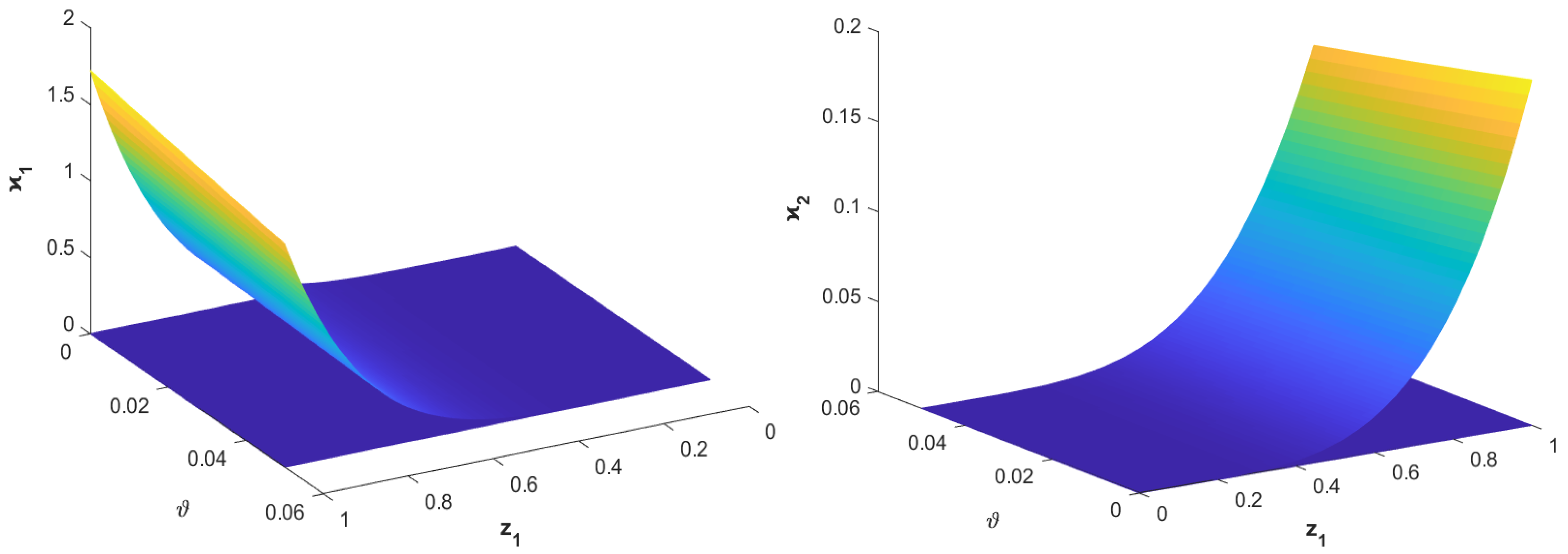
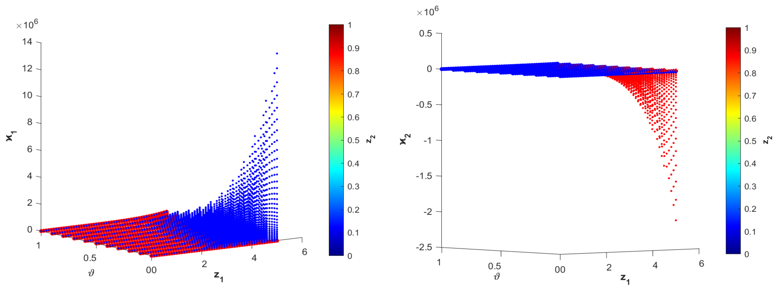
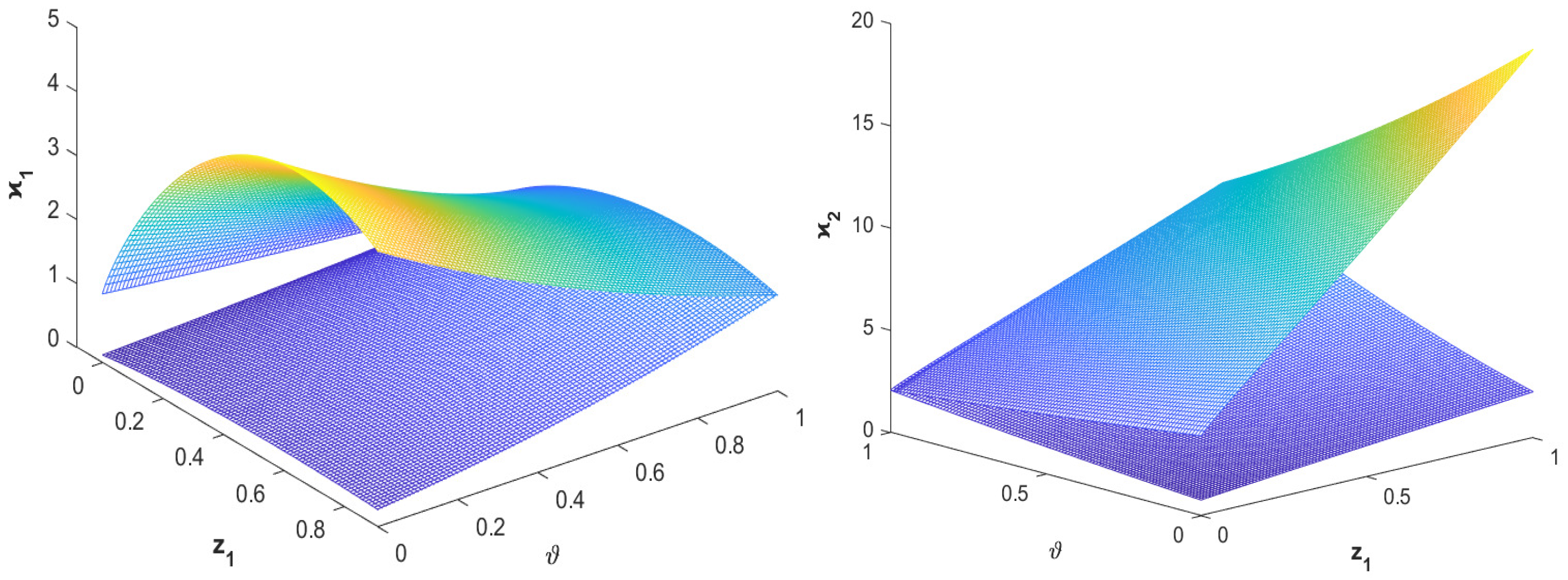
The graphical representation of the fuzzy solution for Example 1 is presented in Figure 1, Figure 2 and Figure 3. Each figure highlights the various aspects of the fuzzy solutions and their associated fuzziness. The graphical representation of the HMF of fuzzy solution ϰ 1 is presented in Figure 1. The time variables z 1 and z 2 are fixed at 1 on the left side, which allows us to observe the fuzziness in ϰ 1 at a specific time instance. The HMF illustrates how this fuzzy solution varies regarding the ϑ -cut and π , with the spread of the function indicating the degree of uncertainty. Higher uncertainty is associated with a greater spread, whereas a narrower spread suggests a more precise solution. When ϑ and π are fixed to 1, the variation of z 1 and z 2 is displayed on the right side of Figure 1. This plot shows how ϰ 1 changes dynamically over time, highlighting how the uncertainty changes as the system behavior changes. Fuzziness and time interact, demonstrating that the system’s uncertainty is dynamic and changes over time. Likewise, Figure 2 displays the graphical representations of fuzzy solutions under the HMF and its temporal variation, ϰ 2 . The variables z 1 and z 2 are fixed to 1 on the left side to provide the graphical depiction of the HMF of ϰ 2 , whereas ϰ 1 shows that the fuzziness is not evenly distributed across the system; the spread of the membership function for ϰ 2 shows the degree of uncertainty. Holding the horizontal membership parameters constant allows the variation in ϰ 2 regarding z 1 and z 2 , displayed on the right side of Figure 2. This figure shows the evolution of ϰ 2 and its fuzziness. The temporal variables ϰ 1 and ϰ 2 behave differently, suggesting that the properties of each solution significantly influence the fuzziness of the systems. Figure 3 shows fuzzy solutions ϰ 1 and ϰ 2 in three dimensions. The uncertainty in ϰ 1 is affected by time and the degree of membership, as seen in ϰ 1 . Additionally, it illustrates the ambiguity between time and fuzziness. By revealing complex patterns in the system’s behavior, the graph emphasizes the need to consider several dimensions while assessing fuzzy systems. On the right side of Figure 3, plotting ϰ 2 under the same conditions provides an alternative perspective regarding the system’s response. This figure highlights the intricate connection between time, fuzziness, and the system’s dynamics. It also provides a more in-depth understanding of the model’s uncertainty. The results demonstrate the importance of considering fuzziness in analyzing continuous fuzzy systems. It is clear from the graphical representations how uncertainty spreads and evolves and the behavior of both time-dependent features and the degree of membership influence the system’s behavior.

5. Applications of FFTDCT Linear System

This section discusses the real-world applications of the proposed granular FFTDCT linear system. The Roesser model is used in signal processing systems because the fuzzy fractional framework efficiently represents the inherent uncertainty of signal components. The second FM model, on the other hand, addresses the challenges of sensor data fusion (SDF) in wireless sensor networks (WSNs) as the reconstruction of the fused sensor state is highly dependent on temporal and spatial uncertainties.

5.1. Application of FFTDCT Linear System Described by the Roesser Model in Signal Processing System

Echo suppression and signal filtering play a crucial role in digital communication and image processing, particularly when uncertainty, fuzziness, memory effects, and spatial distributions influence signal propagation. To model this situation, we consider the Roesser-type granular FFTDCT linear system (17), where the components ϰ 1 ( z 1 , z 2 ) and ϰ 2 ( z 1 , z 2 ) represent the horizontal and vertical signal flow, respectively. Moreover, u ( z 1 , z 2 ) represents the incoming echo/background noise. The matrices A and B are modeled as fuzzy matrices, and the memory effect of the system is described by the fractional orders α 1 = 0.9 and α 2 = 0.8 . This is an important feature in media, where the behavior of the past signals influences the present state. The fuzzy matrices are defined as
A 1 = 1 ˜ 2 ˜ 0 ^ 1 ˜ , and B 1 = 1 ˜ 2 ˜ ,
where 1 ˜ = ( 0.5 , 1 , 1.5 ) , 2 ˜ = ( 1.5 , 2 , 2.5 ) , and 0 ^ = ( 0 , 0 , 0 ) . The matrix A 1 characterizes the impact of the current state and neighboring signal states on the system at every point ( z 1 , z 2 ) , analogous to echo weights in 2D spatial domains. The matrix B 1 captures how the external inputs, including environmental disturbances, influence the system state. The HMFs of the fuzzy matrices given in Equation (51) are
H A 1 = 1 2 + ϑ 2 + ( 1 ϑ ) π 3 2 + ϑ 2 + ( 1 ϑ ) π 0 1 2 + ϑ 2 + ( 1 ϑ ) π , H B 1 = 1 2 + ϑ 2 + ( 1 ϑ ) π 3 2 + ϑ 2 + ( 1 ϑ ) π .
The uncertain initial condition ϰ ( 0 , 0 ) = 1 ˜ represents the signal uncertainty due to measurement errors or external disturbance. The boundary conditions ϰ ( z 1 , 0 ) = ( z 1 , 2 z 1 , 3 z 1 ) and ϰ ( 0 , z 2 ) = ( e z 2 , 2 e z 2 , 3 e z 2 ) define the signal profiles at the boundaries, capturing how the horizontal and vertical input influence propagation. The fuzzy input function simulates an environment with sporadic background signals, including noise bursts or intermittent interference:
u ( z 1 , z 2 ) = 0 ^ , z 1 , z 2 < 0 , 1 ^ , z 1 , z 2 0 .
The HMF of the fuzzy input function is
H u ( z 1 , z 2 ) = 0 , z 1 , z 2 < 0 , 1 , z 1 , z 2 0 .
The following is the fuzzy solution based on Theorem 3
H ϰ 1 ( z 1 , z 2 ) H ϰ 2 ( z 1 , z 2 ) = i = 0 j = 1 H T i j z 1 i α 1 Γ ( 1 + i α 1 ) ( 1 + ϑ + 2 ( 1 ϑ ) π ) e z 2 0 + H b 1 Γ ( ( i + 1 ) α 1 + 1 ) Γ ( j α 2 + 1 ) z 1 ( i + 1 ) α 1 z 2 j α 2 0 + i = 0 H T i 0 z 1 i α 1 Γ ( 1 + i α 1 ) ( 1 + ϑ + 2 ( 1 ϑ ) π ) e z 2 0 + H b 1 Γ ( ( i + 1 ) α 1 + 1 ) z 1 ( i + 1 ) α 1 0 + i = 1 j = 0 H T i j 0 z 2 j α 2 Γ ( 1 + j α 2 ) ( 1 + ϑ + 2 ( 1 ϑ ) π ) z 1 1 + i α 1 Γ ( 2 + i α 1 ) + 0 H b 2 Γ ( i α 1 + 1 ) Γ ( ( j + 1 ) α 2 + 1 ) z 1 i α 1 z 2 ( j + 1 ) α 2 + i = 0 H T 0 j 0 z 1 j α 2 Γ ( 1 + j α 2 ) ( 1 + ϑ + 2 ( 1 ϑ ) π ) z 1 + 0 H b 2 Γ ( ( j + 1 ) α 2 + 1 ) z 2 ( j + 1 ) α 2 .
The plots of the aforementioned fuzzy solution are provided in Figure 4, Figure 5 and Figure 6 with values of i = 25 and j = 25 .
To validate the accuracy of the proposed approach, we compare the analytical fuzzy solution derived in Equation (55) with the approximate solution obtained using the fuzzy fractional forward Euler method. The values of the fractional orders, fuzzy parameters, and uncertain initial and boundary conditions used in this comparison are specified in Section 5.1. Table 2 presents the numerical results for both the analytical and approximate solutions of ϰ 1 ( z 1 , z 2 , ϑ , π ) (hereafter referred to as ϰ 1 ) and ϰ 2 ( z 1 , z 2 , ϑ , π ) (hereafter referred to as ϰ 2 ). In the table, ϰ 1 Analytic and ϰ 2 Analytic denote the analytical solutions of ϰ 1 and ϰ 2 , respectively, while ϰ 1 m a t h r m A p p r o x . and ϰ 2 Approx . represent the corresponding approximate solutions obtained via the numerical method.
Now, we calculate the pointwise absolute and relative errors between the analytical and approximate solutions. Table 3 presents the error analysis results for both ϰ 1 and ϰ 2 . The pointwise absolute error (AE) is computed using the formula
AE = ϰ Analytic ϰ Approx . ,
while the pointwise relative error (RE) is given by
RE = ϰ Analytic ϰ Approx . ϰ Analytic .
These metrics enable a quantitative comparison of the numerical approximation with the exact fuzzy analytical solution.
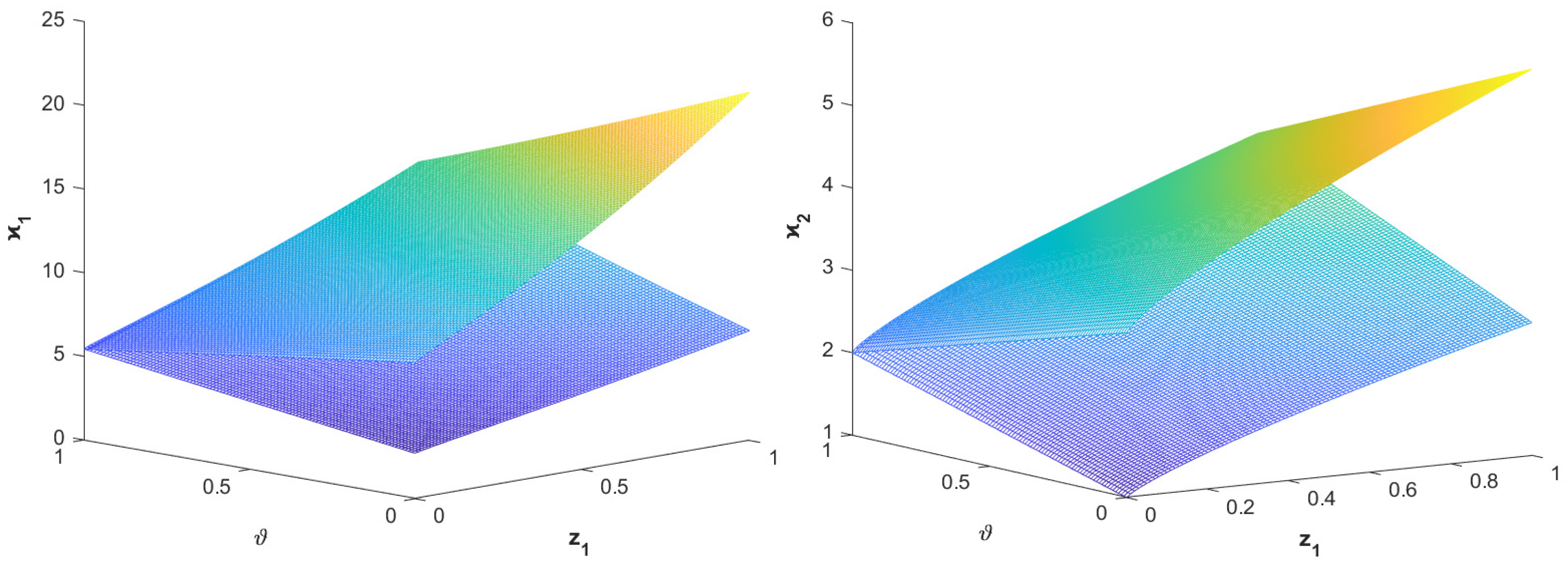
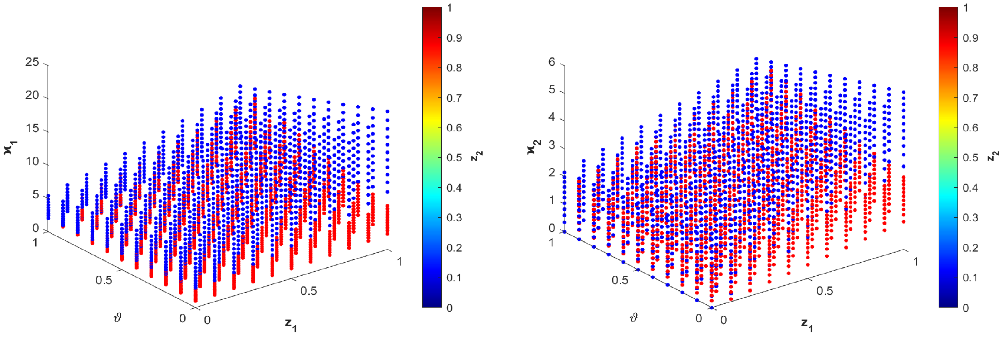
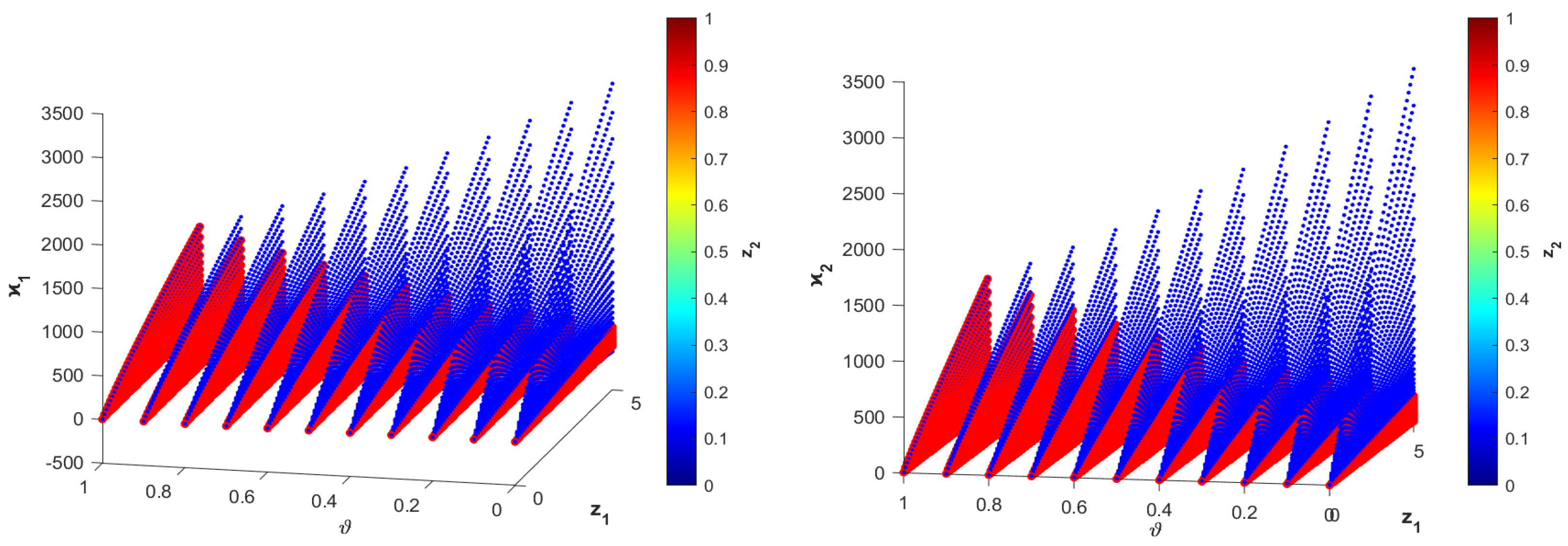
Figure 4 shows the graphical visualization of the components ϰ 1 ( z 1 , z 2 ) and ϰ 2 ( z 1 , z 2 ) by taking ϑ = 1 and π = 1 . These figures illustrate the evolution of the fuzzy fractional signal under uncertain environments. Here, π = 1 ensures that the horizontal membership distribution spans its entire range, indicating the system’s maximum predicted response. In this scenario, ϑ = 1 captures the crisp core of the fuzzy solution. Both ϰ 1 ( z 1 , z 2 ) and ϰ 2 ( z 1 , z 2 ) represent distinct components of a processed signal, each influenced by internal system feedback and external disturbances, with their behavior modeled using fuzzy and fractional parameters. The smooth and increasing trend of both surfaces shows a stable signal evolution, where the system efficiently captures both attenuation and amplification in response to changes in z 1 and z 2 . This behavior represents the signal processing scenario in an uncertain environment, including echo suppression, where the memory effect and fuzziness are inherent. The graphical representation indicates that the system remains bounded and predictable, which is essential for practical signal reconstruction and enhancement. Figure 5 represents the graphical behavior of the fuzzy solutions of the components ϰ 1 ( z 1 , 1 , ϑ ) and ϰ 2 ( 1 , z 2 , ϑ ) , indicating the smooth and continuous surfaces. This confirms the stable behavior of the system with fractional orders α 1 = 0.9 and α 2 = 0.8 . The proposed solution captures the expected uncertainty propagation in a fuzzy environment. These graphical representations demonstrate that the fractional orders and fuzzy parameters jointly influence the flexibility of the system and memory effect. Figure 6 provides graphical representations of fuzzy solutions ϰ 1 ( z 1 , z 2 , ϑ ) and ϰ 2 ( z 1 , z 2 , ϑ ) . The left and right figures show the four-dimensional scatter plots of fuzzy solutions ϰ 1 ( z 1 , z 2 , ϑ ) and ϰ 2 ( z 1 , z 2 , ϑ ) , respectively. In Figure 6, the red points represent the left bound, and the blue points represent the right bound of the ϑ -cut of the FVF. This graphical representation illustrates how the uncertainty varies between input parameters for fixed fractional orders α 1 = 0.9 and α 2 = 0.8 , offering insight into its spread and behavior.

5.2. Application of FFTDCT Linear System in Wireless Sensor Network Data Fusion

Now, we apply the proposed model (33) to describe the problem of SDF in WSNs in a fuzzy environment. In real-world applications, spatially distributed sensors in a geographic region monitor conditions, including temperature, air quality, or humidity in a 2D space. Sensor readings usually exhibit uncertainty due to hardware constraints, latency in data transmission, and external interference. These properties are naturally described using fuzzy numbers, while fractional-order derivatives well model the memory-dependent characteristic of physical processes. The uncertain dynamics of the SDF of the WSN can be well captured by the proposed system (33), where ϰ ( z 1 , z 2 ) represents the fused sensor state within the spatial coordinates z 1 and z 2 . u ( z 1 , z 2 ) describes an external control or input source, including the sensor reading’s emission signal or distributed activations. In our simulation, we assume the fractional orders α 1 = 0.9 and α 2 = 0.8 to capture the inherent long-memory dynamics and the delayed spatial interaction observed in transmission of WSN data. The fuzzy system matrices and its HMF are defined in Equations (46) and (47), where 1 ˜ = ( 0.5 , 1 , 1.5 ) in Equation (46) represents fuzzy measurements and 0 ^ = ( 0 , 0 , 0 ) indicates perfect certainty at zero. We consider the fuzzy initial condition ϰ ( 0 , 0 ) = 1 ˜ and the fuzzy boundary conditions ϰ ( z 1 , 0 ) = ( z 1 , 2 z 1 , 3 z 1 ) and ϰ ( 0 , z 2 ) = ( e z 2 , 2 e z 2 , 3 e z 2 ) for the SDF problem in WSNs to describe the initial uncertainty and horizontal and vertical boundary profile, respectively. The fuzzy input formulation in Equation (54) describes the activation state of the sensors when z 1 , z 2 0 and their inactivity in unobservable regions. The HMF of the fuzzy input function is given in Equation (54). According to Theorem 3, the fuzzy solution is given in the following:
H ϰ ( z 1 , z 2 ) = i = 0 j = 0 ( H T i j ( 1 2 + ϑ 2 ( 1 ϑ ) π ) t 1 i α 1 t 2 j α 2 Γ ( i α 1 + 1 ) Γ ( i α 2 + 1 ) H T i j H B 1 t 1 i α 1 Γ ( i α 1 + 1 ) 1 Γ ( ( j + 1 ) α 2 ) 0 z 2 ( z 2 τ 2 ) ( j + 1 ) α 2 1 d τ 2 H T i j H B 2 t 2 j α 2 Γ ( j α 2 + 1 ) 1 Γ ( ( i + 1 ) α 1 ) 0 z 1 ( z 1 τ 1 ) ( i + 1 ) α 1 1 d τ 1 + H T i , j 1 H A 1 t 2 j α 2 Γ ( j α 2 + 1 ) 1 Γ ( ( i α 1 ) ) 0 z 1 ( z 1 τ 1 ) i α 1 1 ( 1 + ϑ + 2 ( 1 ϑ ) π ) τ 1 d τ 1 + H T i 1 , j H A 2 t 1 i α 1 Γ ( i α 1 + 1 ) 1 Γ ( ( j α 2 ) ) 0 z 2 ( z 2 τ 2 ) j α 2 1 ( 1 + ϑ + 2 ( 1 ϑ ) π ) e τ 2 d τ 2 + [ H T i , j 1 H B 1 + H T i 1 , j H B 2 ] 1 Γ ( i α 1 ) Γ ( j α 2 ) 0 z 1 0 z 2 ( z 1 τ 1 ) i α 1 1 ( z 2 τ 2 ) j α 2 1 d τ 1 d τ 2 ) .
After performing the integral in Equation (56) and simplifying the resulting expression, we obtain the following:
H ϰ ( z 1 , z 2 ) = i = 0 j = 0 ( H T i j ( 1 2 + ϑ 2 ( 1 ϑ ) π ) t 1 i α 1 t 2 j α 2 Γ ( i α 1 + 1 ) Γ ( i α 2 + 1 ) H T i j H B 1 t 1 i α 1 t 2 ( j + 1 ) α 2 Γ ( i α 1 + 1 ) Γ ( ( j + 1 ) α 2 ) H T i j H B 2 t 1 ( i + 1 ) α 1 t 2 j α 2 Γ ( j α 2 + 1 ) Γ ( ( i + 1 ) α 1 ) + H T i , j 1 H A 1 t 2 j α 2 Γ ( j α 2 + 1 ) ( 1 + ϑ + 2 ( 1 ϑ ) π ) t 1 1 + i α 1 Γ ( 2 + i α 1 ) + H T i 1 , j H A 2 t 1 i α 1 Γ ( i α 1 + 1 ) ( 1 + ϑ + 2 ( 1 ϑ ) π ) e z 2 + [ H T i , j 1 H B 1 + H T i 1 , j H B 2 ] t 1 i α 1 t 2 j α 2 Γ ( i α 1 + 1 ) Γ ( j α 2 + 1 ) ) .
To validate the proposed fuzzy solution of the system (33), we compare it with the classical solution provided by Rogowski in [45]. The classical solution of system (33) is given as
ϰ ( z 1 , z 2 ) = i = 0 j = 0 ( T i j t 1 i α 1 Γ ( i α 1 + 1 ) t 2 j α 2 Γ ( i α 2 + 1 ) ϰ ( 0 , 0 ) T i j B 1 t 1 i α 1 Γ ( i α 1 + 1 ) 1 Γ ( ( j + 1 ) α 2 ) 0 z 2 ( z 2 τ 2 ) ( j + 1 ) α 2 1 u ( 0 , τ 2 ) d τ 2 T i j B 2 t 2 j α 2 Γ ( j α 2 + 1 ) 1 Γ ( ( i + 1 ) α 1 ) 0 z 1 ( z 1 τ 1 ) ( i + 1 ) α 1 1 u ( τ 1 , 0 ) d τ 1 + T i , j 1 A 1 t 2 j α 2 Γ ( j α 2 + 1 ) 1 Γ ( ( i α 1 ) ) 0 z 1 ( z 1 τ 1 ) i α 1 1 ϰ ( τ 1 , 0 ) d τ 1 + T i 1 , j A 2 t 1 i α 1 Γ ( i α 1 + 1 ) 1 Γ ( ( j α 2 ) ) 0 z 2 ( z 2 τ 2 ) j α 2 1 ϰ ( 0 , τ 2 ) d τ 2 + [ T i , j 1 B 1 + T i 1 , j B 2 ] 1 Γ ( i α 1 ) Γ ( j α 2 ) 0 z 1 0 z 2 ( z 1 τ 1 ) i α 1 1 ( z 2 τ 2 ) j α 2 1 u ( τ 1 , τ 2 ) d τ 1 d τ 2 ) .
Here, the coefficient matrices are defined as
A 1 = 1 2 0 1 , and B 1 = 1 2 ,
with the initial condition ϰ ( 0 , 0 ) = 1 , and boundary conditions ϰ ( z 1 , 0 ) = 2 z 1 and ϰ ( 0 , z 2 ) = 2 e z 2 . This classical solution coincides with the fuzzy solution in Equation (57) when the fuzzification parameter is ϑ = 1 . To illustrate the impact of fuzzification, we modify the initial condition to ϰ ( 0 , 0 ) = 1.1 and the boundary conditions to ϰ ( z 1 , 0 ) = 2.1 z 1 and ϰ ( 0 , z 2 ) = 2.1 e z 2 . With these changes, the classical solution in Equation (58) corresponds to the fuzzy solution with ϑ = 0.99 . This comparative analysis demonstrates that the fuzzy analytical solution generalizes the crisp solution and allows a tolerance-based interpretation of the model. Therefore, the fuzzification of this system offers greater flexibility in modeling uncertainty and enhances its practical applicability.
Figure 7 illustrates the graphical representations of the fuzzy solution in terms of HMFs of fused sensor states ϰ 1 and ϰ 2 under the granular FFTDCT linear system for fixed spatial coordinates z 1 = 1 and z 2 = 1 . The graph explores the dynamic behavior of the HMF as a solution function of two important parameters, ϑ and π . The ϑ -level represents the confidence level in the fuzzy measurement, with values ranging from 0 to 1. Moreover, π represents the RDM that captures the spatial or environmental variations that affect the sensor data. The parameter π governs the influence of environmental effects, which means that a higher value of π can represent conditions where sensors are deployed in large areas or highly variable surroundings. Figure 8 illustrates the graphical representations of the fuzzy solutions of ϰ 1 ( z 1 , 1 , ϑ ) and ϰ 2 ( z 1 , 1 , ϑ ) . The graphs perfectly represent the triangular fuzzy nature of the FSD. Figure 8 captures the degree of fuzziness in the fused sensor state at a specific location z 1 for a fixed z 2 . For every ϑ -level value, the plot shows the confidence interval in the fusion output. At ϑ = 0 , the solution exhibits the widest uncertainty bounds, capturing the maximum fuzziness in the fused state. As ϑ -level values increase, the endpoints narrow, indicating greater confidence with reduced uncertainty. The system converges to the deterministic solution at ϑ = 1 , where the fuzzy bounds collapse with single crisp values. This visualization illustrates how a WSN system enhances its fusion output by reducing uncertainty. Figure 9 presents the graphical representations of the fuzzy fusion solutions ϰ 1 ( z 1 , z 2 , ϑ ) and ϰ 2 ( z 1 , z 2 , ϑ ) for WSN data fusion under uncertainty. Each point represents the potential state of the FSD corresponding to the different values of the ϑ -cut levels. The red points represent the lower bound of the sensor fusion outcome, and the blue points indicate the upper end of the v a r t h e t a -cut. This four-dimensional graph illustrates how the fused sensor output varies across the spatial positions ( z 1 , z 2 ) and the confidence level, highlighting the presence of environmental and sensor-induced uncertainty on the system behavior. This visualization allows the decision-makers in WSN-based systems, including environmental sensing and industrial monitoring, to understand the range of possible fused sensor outputs and sensor confidence.

6. Conclusions

In this article, two classes of FFTDCT linear systems were introduced and investigated to address uncertainty and fuzziness in the system parameters. Firstly, the FFTDCT linear systems described by the Roesser model were analyzed. The potential solution of the fuzzy fractional system was extracted using a 2D granular Laplace transform approach. Secondly, the FFTDCT linear systems described by the second FM model structure were investigated, where the state-space equations contain two-dimensional and one-dimensional partial fractional-order Caputo derivatives. The fuzzy solution of the proposed models was obtained by using the 2D granular Laplace transform. The numerical examples were solved to support the theoretical developments.
The proposed study provides a structured approach for analyzing fuzzy fractional-order TDLSs under uncertainty, bridging the gap between traditional deterministic models and real-world applications where uncertainty is inherent.

Author Contributions

Concept, design, analysis, writing (original draft, review and editing), and revision of the manuscript: G.M., M.A., H.A. and N.H. All authors have read and agreed to the published version of the manuscript.

Funding

This research received no external funding.

Data Availability Statement

The original contributions presented in this study are included in the article. Further inquiries can be directed to the corresponding author(s).

Conflicts of Interest

The authors declare no conflicts of interest.

References

  1. Zeng, G.; Chen, S.; Wu, H.; Yang, M. Continuous-discrete extended Kalman filtering based on the neural ordinary differential equations method. Eng. Appl. Artif. Intell. 2024, 133, 108611. [Google Scholar] [CrossRef]
  2. Dubois, D.; Prade, H. Towards fuzzy differential calculus part 3: Differentiation. Fuzzy Sets Syst. 1982, 8, 225–233. [Google Scholar] [CrossRef]
  3. Akram, M.; Muhammad, G.; Allahviranloo, T.; Pedrycz, W. Solution of initial-value problem for linear third-order fuzzy differential equations. Comput. Appl. Math. 2022, 41, 398. [Google Scholar] [CrossRef]
  4. Muhammad, G.; Akram, M. Fuzzy fractional epidemiological model for Middle East respiratory syndrome coronavirus on complex heterogeneous network using Caputo derivative. Inf. Sci. 2024, 659, 120046. [Google Scholar] [CrossRef]
  5. Muhammad, G.; Akram, M. Fuzzy fractional generalized Bagley-Torvik equation with fuzzy Caputo gH-differentiability. Eng. Appl. Artif. Intell. 2024, 133, 108265. [Google Scholar] [CrossRef]
  6. Akram, M.; Muhammad, G.; Allahviranloo, T. Explicit analytical solutions of an incommensurate system of fractional differential equations in a fuzzy environment. Inf. Sci. 2023, 645, 119372. [Google Scholar] [CrossRef]
  7. Akram, M.; Muhammad, G.; Allahviranloo, T.; Pedrycz, W. Incommensurate non-homogeneous system of fuzzy linear fractional differential equations using the fuzzy bunch of real functions. Fuzzy Sets Syst. 2023, 473, 108725. [Google Scholar] [CrossRef]
  8. Mazandarani, M.; Pan, J. The challenges of modeling using fuzzy standard interval arithmetic: A case study in electrical engineering. Inf. Sci. 2024, 653, 119774. [Google Scholar] [CrossRef]
  9. Mazarani, M.; Pariz, N.; Kamyad, A.V. Granular differentiability of fuzzy-number-valued functions. IEEE Trans. Fuzzy Syst. 2017, 26, 310–323. [Google Scholar] [CrossRef]
  10. Cano, Y.C.; Flores, H.R. On new solutions of fuzzy differential equations. Chaos Solitons Fractals 2008, 38, 112–119. [Google Scholar] [CrossRef]
  11. Roesser, R. A discrete state-space model for linear image processing. IEEE Trans. Autom. Control 1975, 20, 1–10. [Google Scholar] [CrossRef]
  12. Fornasini, E.; Marchesini, G. State-space realization theory of two-dimensional filters. IEEE Trans. Autom. Control 1976, 21, 484–491. [Google Scholar] [CrossRef]
  13. Kurek, J. The general state-space model for two-dimensional linear digital systems. IEEE Trans. Autom. Control 1985, 30, 600–602. [Google Scholar] [CrossRef]
  14. Bose, N.K. Applied Multidimensional Systems Theory; Van Nostrand Reinhold Co.: New York, NY, USA, 1982. [Google Scholar]
  15. Kaczorek, T. Two-Dimensional Linear Systems; Springer: London, UK, 1985. [Google Scholar]
  16. Galkowski, K. State-Space Realizations of Linear 2-D Systems with Extensions to the General nD (n > 2) Case; Springer: London, UK, 2001. [Google Scholar]
  17. Farina, L.; Rinaldi, S. Positive Linear Systems: Theory and Applications; John Wiley & Sons: New York, NY, USA, 2000. [Google Scholar]
  18. Oldham, K.B.; Spanier, J. The Fractional Calculus; Academic Press: New York, NY, USA, 1974. [Google Scholar]
  19. Miller, K.S.; Ross, B. An Introduction to the Fractional Calculus and Fractional Differential Equations; John Wiley & Sons: New York, NY, USA, 1993. [Google Scholar]
  20. Podlubny, I. Fractional Differential Equations; Academic Press: London, UK, 1999. [Google Scholar]
  21. Kaczorek, T. Fractional 2D linear systems. J. Autom. Mob. Robot. Intell. Syst. 2008, 2, 5–9. [Google Scholar]
  22. Rogowski, K. General response formula for fractional 2D continuous-time linear systems described by the Roesser model. Acta Mech. Autom. 2011, 5, 112–116. [Google Scholar]
  23. Kaczorek, T.; Rogowski, K. Fractional Linear Systems and Electrical Circuits; Springer International Publishing: Cham, Switzerland, 2015; pp. 49–80. [Google Scholar]
  24. Rogowski, K. Selected Problems of Theory of 2D Non-Integer Order Systems Described by the Roesser Model. Ph.D. Thesis, Bialystok University of Technology, Bialystok, Poland, 2011. (In Polish). [Google Scholar]
  25. Idczak, M.; Kamocki, T.; Majewski, M. On a fractional continuous counterpart of Fornasini-Marchesini model. In Proceedings of the International Conference on Multidimensional Systems, Erlangen, Germany, 9–11 September 2013; pp. 1–5. [Google Scholar]
  26. Rogowski, K. Positivity analysis of continuous Fornasini-Marchesini fractional model. In Proceedings of the 5th International Symposium on Positive Systems, Rome, Italy, 14–16 September 2016. [Google Scholar]
  27. Hu, H.; Meng, Y.; Huang, S. Dynamic event-triggered control of 2-D continuous systems in Roesser model. Asian J. Control 2025, 27, 646–660. [Google Scholar] [CrossRef]
  28. Huang, Y.; Wu, B.; Wang, Y.E.; Liu, L. Practical exponential stability of switched generalized homogeneous positive nonlinear systems with bounded disturbances. Circuits Syst. Signal Process. 2025, 44, 3793–3809. [Google Scholar] [CrossRef]
  29. Ma, H.; Tian, D.; Li, M.; Zhang, C. Reachable set estimation for 2-D switched nonlinear positive systems with impulsive effects and bounded disturbances described by the Roesser model. Math. Model. Control 2024, 4, 152–162. [Google Scholar] [CrossRef]
  30. Dami, L.; Benzaouia, A. Stabilization of switched two dimensional fractional order positive systems modeled by the Roesser model. J. Control Autom. Electr. Syst. 2023, 34, 1136–1144. [Google Scholar] [CrossRef]
  31. Huang, S.; Yan, Z.; Zhang, Z.; Zeng, G. Finite-time boundedness of two-dimensional positive continuous-discrete systems in Roesser model. Trans. Inst. Meas. Control 2021, 43, 1452–1463. [Google Scholar] [CrossRef]
  32. Gao, J.; Wang, W.; Zhang, G. Finite-time stability and control of 2D continuous–discrete systems in Roesser model. Circuits Syst. Signal Process. 2018, 37, 4789–4809. [Google Scholar] [CrossRef]
  33. Ahn, C.K.; Shi, P.; Wu, L. l-gain performance analysis for two-dimensional Roesser systems with persistent bounded disturbance and saturation nonlinearity. Inf. Sci. 2016, 333, 126–139. [Google Scholar] [CrossRef]
  34. Nemati, A.; Mamehrashi, K. The use of the Ritz method and Laplace transform for solving 2D fractional-order optimal control problems described by the Roesser model. Asian J. Control 2019, 21, 1189–1201. [Google Scholar] [CrossRef]
  35. Zhang, J.R.; Lu, J.G.; Zhu, Z. Stability analysis and stabilisation of continuous-discrete fractional-order 2D Fornasini-Marchesini first model. Int. J. Syst. Sci. 2023, 54, 333–344. [Google Scholar] [CrossRef]
  36. Zhu, Z.; Lu, J.G. Robust stability and stabilization of continuous-discrete fractional-order 2D Fornasini-Marchesini second model with interval uncertainties. Asian J. Control 2024, 26, 3054–3066. [Google Scholar] [CrossRef]
  37. Zhang, G.; Wang, W. Finite-region stability and boundedness for discrete 2D Fornasini-Marchesini second models. Int. J. Syst. Sci. 2017, 48, 778–787. [Google Scholar] [CrossRef]
  38. Benyettou, K.; Bouagada, D.; Ghezzar, M.A. Solution of 2D state space continuous-time conformable fractional linear system using Laplace and Sumudu transform. Comput. Math. Model. 2021, 32, 94–109. [Google Scholar] [CrossRef]
  39. Benyettou, K.; Bouagada, D.; Benamar, M.N. Controllability and minimum energy control problem of two-dimensional continuous-time fractional linear systems. Int. J. Syst. Sci. 2024, 56, 966–981. [Google Scholar] [CrossRef]
  40. Yan, S.; Sun, L.; Xu, L.; Cai, Y.; Zhao, Q. State-space formulation of 2-D frequency transformation in Fornasini-Marchesini second model. Multidimens. Syst. Signal Process. 2018, 29, 361–383. [Google Scholar] [CrossRef]
  41. Li, X.; Hou, X. Design of parametric controller for two-dimensional polynomial systems described by the Fornasini-Marchesini second model. IEEE Access 2019, 7, 44070–44079. [Google Scholar] [CrossRef]
  42. Bede, B.; Stefanini, L. Generalized differentiability of fuzzy-valued functions. Fuzzy Sets Syst. 2013, 230, 119–141. [Google Scholar] [CrossRef]
  43. Son, N.T.K.; Long, H.V.; Dong, N.P. Fuzzy delay differential equations under granular differentiability with applications. Comput. Appl. Math. 2019, 38, 107. [Google Scholar] [CrossRef]
  44. Kaczorek, T. Selected Problems in Fractional Systems Theory; Springer: London, UK, 2011. [Google Scholar]
  45. Rogowski, K. Solution to the fractional-order 2D continuous systems described by the second Fornasini-Marchesini model. IFAC-PapersOnLine 2017, 50, 9748–9752. [Google Scholar] [CrossRef]
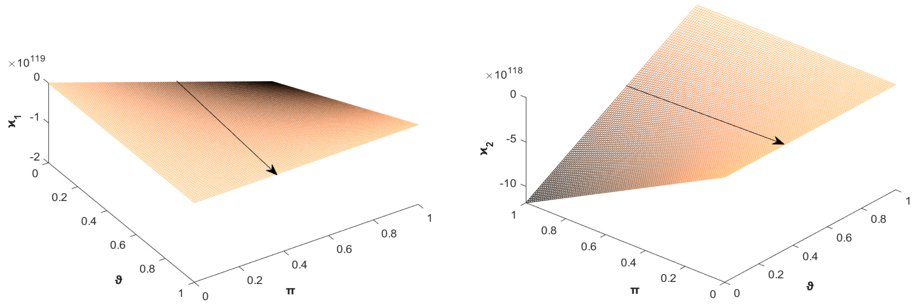
Figure 1. The left figure shows HMFs of ϰ 1 ( z 1 , z 2 ) , and the right figure shows the HMFs of ϰ 2 ( z 1 , z 2 ) for different values of ϑ and π by fixing z 1 = z 2 = 1 .
Fractalfract 09 00398 g001
Figure 2. Graphical representations of fuzzy solutions ϰ 1 ( z 1 , 1 , ϑ ) and ϰ 2 ( z 1 , 1 , ϑ ) , respectively.
Fractalfract 09 00398 g002
Figure 3. The left and right figures show the four-dimensional scatter plots of fuzzy solutions ϰ 1 ( z 1 , z 2 , ϑ ) and ϰ 2 ( z 1 , z 2 , ϑ ) , respectively. The red points represent the left bound, and the blue points represent the right bound of the ϑ -cut of the FVF.
Fractalfract 09 00398 g003
Figure 4. The left and right figures show the graphical representations of ϰ 1 ( z 1 , z 2 ) and ϰ 2 ( z 1 , z 2 ) for different values of z 1 and z 2 by fixing ϑ and π .
Fractalfract 09 00398 g004
Figure 5. The left and right figures show the graphical representations of fuzzy solutions ϰ 1 ( z 1 1 , ϑ ) and ϰ 2 ( 1 , z 2 , ϑ ) , respectively.
Fractalfract 09 00398 g005
Figure 6. The left and right figures show the four-dimensional scatter plots of fuzzy solutions ϰ 1 ( z 1 , z 2 , ϑ ) and ϰ 2 ( z 1 , z 2 , ϑ ) , respectively. The red points represent the left bound, and the blue points represent the right bound of the ϑ -cut of the FVF.
Fractalfract 09 00398 g006
Figure 7. The graphical representation of HMFs of ϰ 1 and ϰ 2 for fixing the values z 1 = 1 and z 2 = 1 (left to right), respectively.
Fractalfract 09 00398 g007
Figure 8. Graphical representations of fuzzy solutions ϰ 1 ( z 1 , 1 , ϑ ) and ϰ 2 ( z 1 , 1 , ϑ ) , respectively.
Fractalfract 09 00398 g008
Figure 9. The left and right figures show the four-dimensional scatter plots of fuzzy solutions ϰ 1 ( z 1 , z 2 , ϑ ) and ϰ 2 ( z 1 , z 2 , ϑ ) , respectively. The red points represent the left bound, and the blue points represent the right bound of the ϑ -cut of the FVF.
Fractalfract 09 00398 g009
Table 1. Summary of notations.
Notation DescriptionLocation
Ξ R The collection of all FNs on R Section 2
H ( m ) m gr ( ϑ , π ) The HMF of the FN m Ξ R Section 2
I z i α i The 2DRL fractional integral of order α i regarding the variable z i (i = 1, 2)Definition 9
D z i α i C The 2D Caputo fractional derivative (CFD) of order α i > 0 regarding variable z i   ( i = 1 , 2 ) Definition 12
L z 1 , z 2 The 2D Laplace transform regarding z 1 and z 2 Definition 16
L z 1 , z 2 The 2D granular Laplace transform regarding z 1 and z 2 Definition 18
I z i α i gr The GFI of order α i regarding z i (i = 1, 2)Definition 13
D z i α i gr The two-dimensional GCFD of order α i > 0 regarding z i (i = 1, 2)Definition 14
I z 1 α ϰ ( z 1 , z 2 ) FI of order α > 0 of ϰ ( z 1 , z 2 ) regarding the
variable z 1
Definition 8
Table 2. The numerical values of the analytical and approximate solutions of ϰ 1 and ϰ 2 .
z 1 z 2 ϑ π ϰ 1 Analytic ϰ 2 Analytic ϰ 1 Approx . ϰ 2 Approx .
0.00.00.00.00.51230.51010.51120.5100
0.10.10.10.10.24390.35010.24220.3452
0.20.20.20.20.72010.81120.71990.8108
0.30.30.30.31.56071.41401.56021.4112
0.40.40.40.42.89692.17152.89502.1612
0.50.50.50.54.85013.18394.84993.1822
0.60.60.60.67.58994.19307.58124.1901
0.70.70.70.711.14835.392911.14605.3924
0.80.80.80.815.50376.653015.50016.6501
0.90.90.90.920.99877.853520.99407.8427
1.01.01.01.024.93398.818524.83128.8130
Table 3. Absolute and relative errors between analytical and approximate solutions of ϰ 1 and ϰ 2 .
ϰ 1 - Analytic ϰ 1 - Approx . AE ϰ 1 RE ϰ 1 ϰ 2 - Analytic ϰ 2 - Approx . AE ϰ 2 RE ϰ 2
0.51230.51120.00110.0021470.51010.51000.00010.000196
0.24390.24220.00170.0069700.35010.34520.00490.014000
0.72010.71990.00020.0002780.81120.81080.00040.000493
1.56071.56020.00050.0003201.41401.41120.00280.001982
2.89692.89500.00190.0006562.17152.16120.01030.004740
4.85014.84990.00020.0000413.18393.18220.00170.000533
7.58997.58120.00870.0011464.19304.19010.00290.000693
11.148311.14600.00230.0002065.39295.39240.00050.000093
15.503715.50010.00360.0002326.65306.65010.00290.000437
20.998720.99400.00470.0002247.85357.84270.01080.001375
24.933924.83120.10270.0041198.81858.81300.00550.000623
Disclaimer/Publisher’s Note: The statements, opinions and data contained in all publications are solely those of the individual author(s) and contributor(s) and not of MDPI and/or the editor(s). MDPI and/or the editor(s) disclaim responsibility for any injury to people or property resulting from any ideas, methods, instructions or products referred to in the content.