Optimizing Load Frequency Control of Multi-Area Power Renewable and Thermal Systems Using Advanced Proportional–Integral–Derivative Controllers and Catch Fish Algorithm

Abstract

Renewable energy sources (RESs) are increasingly combined into the power system due to market liberalization and environmental and economic benefits, but their weather-dependent variability causes power production and demand mismatches, leading to issues like frequency and regional power transmission fluctuations. To maintain synchronization in power systems, frequency must remain constant; disruptions in the proper balance of production and load might produce frequency variations, risking serious issues. Therefore, a mechanism known as load frequency control (LFC) or automated generation control (AGC) is needed to keep the frequency and tie-line power within predefined stable limits. In this study, advanced proportional–integral–derivative PID controllers such as fractional-order PID (FOPID), cascaded PI(PDN), and PI(1+DD) for LFC in a two-area power system integrated with RES are optimized using the catch fish optimization algorithm (CFA). The controllers’ optimal gains are attained through using the integral absolute error (IAE) and ITAE objective functions. The performance of LFC with CFA-tuned PID, PI, cascaded PI(PDN), and FOPID, PI(1+DD) controllers is compared to other optimization techniques, including sine cosine algorithm (SCA), particle swarm optimization (PSO), brown bear algorithm (BBA), and grey wolf optimization (GWO), in a two-area power system combined with RESs under various conditions. Additionally, by contrasting the performance of the PID, PI, cascaded PI(PDN), and FOPID, PI(1+DD) controllers, the efficiency of the CFA is confirmed. Additionally, a sensitivity analysis that considers simultaneous modifications of the frequency bias coefficient (B) and speed regulation (R) within a range of ±25% validates the efficacy and dependability of the suggested CFA-tuned PI(1+DD). In the complex dynamics of a two-area interconnected power system, the results show how robust the suggested CFA-tuned PI(1+DD) control strategy is and how well it can stabilize variations in load frequency and tie-line power with a noticeably shorter settling time. Finally, the results of the simulation show that CFA performs better than the GWO, BBA, SCA, and PSO strategies.

1. Introduction

A major issue facing rural settlements is the lack of easily accessible electrical power. They are geographically isolated, which contributes to the impracticability of the traditional grid’s extension. The advance of RESs has increased at the national and local levels due to increasing requirements for power, the limited availability of fossil fuels, and growing environmental concerns [1,2,3]. The optimal power flow, the quality of power, voltage and frequency control, and other aspects are all impacted by the unpredictable nature of RES. Making sure that the electric power system’s (EPS) conventional frequency and voltage output stay constant is the primary goal of experts who work diligently in the industry. Any deterioration in any of these two attributes would have an adverse effect on the power system’s associated equipment’s productivity and anticipated lifetime [4,5,6,7].

Many power production sources, including nuclear power, fuel, thermal energy, hydro power, solar, wind, and management regions, are typically connected via tie-lines to form an integrated power system. The power grid’s primary components include distribution networks, transmission lines, and generating networks, some of which may use RESs. Furthermore, variations in active and reactive power requirements may result from the integration and functioning of various components in real-time. A shift in the system frequency occurs when there is an imbalance between the power produced via the generators and the power demanded by the consumers. When the electricity generated surpasses the power used, the frequency rises. However, if more power is required than is generated, the frequency decreases. Abnormal oscillations brought on by these systemic variances must be removed. If not, there may be negative effects on the power system’s process and even system breakdowns. To preserve the system frequency deviations and tie-line power oscillations in the set bounds, a control procedure identified as an LFC or an AGC is necessary [8,9,10].

In order to maintain production–consumption balancing in the event of load fluctuations, current power systems need to be very intelligent and flexible during the management and optimization processes. Conventional energy sources are insufficient to provide the needed load balancing, as seen by the steady decline in fossil fuels and price increases for fuel [11,12]. In order to fulfill the growing load requirements, it is therefore essential to combine conventional power sources with RESs. In modern power systems, photovoltaic (PV) modules and wind turbine plants (WT) are the most common energy sources. However, deviations in frequency are brought on by the imbalance between consumption and production brought on by the uncertainty inherent in RESs, such as oscillations in wind velocity and variations in solar radiation. In this instance, keeping deviations from frequency within the intended ranges is mostly dependent on the LFC/AGC. 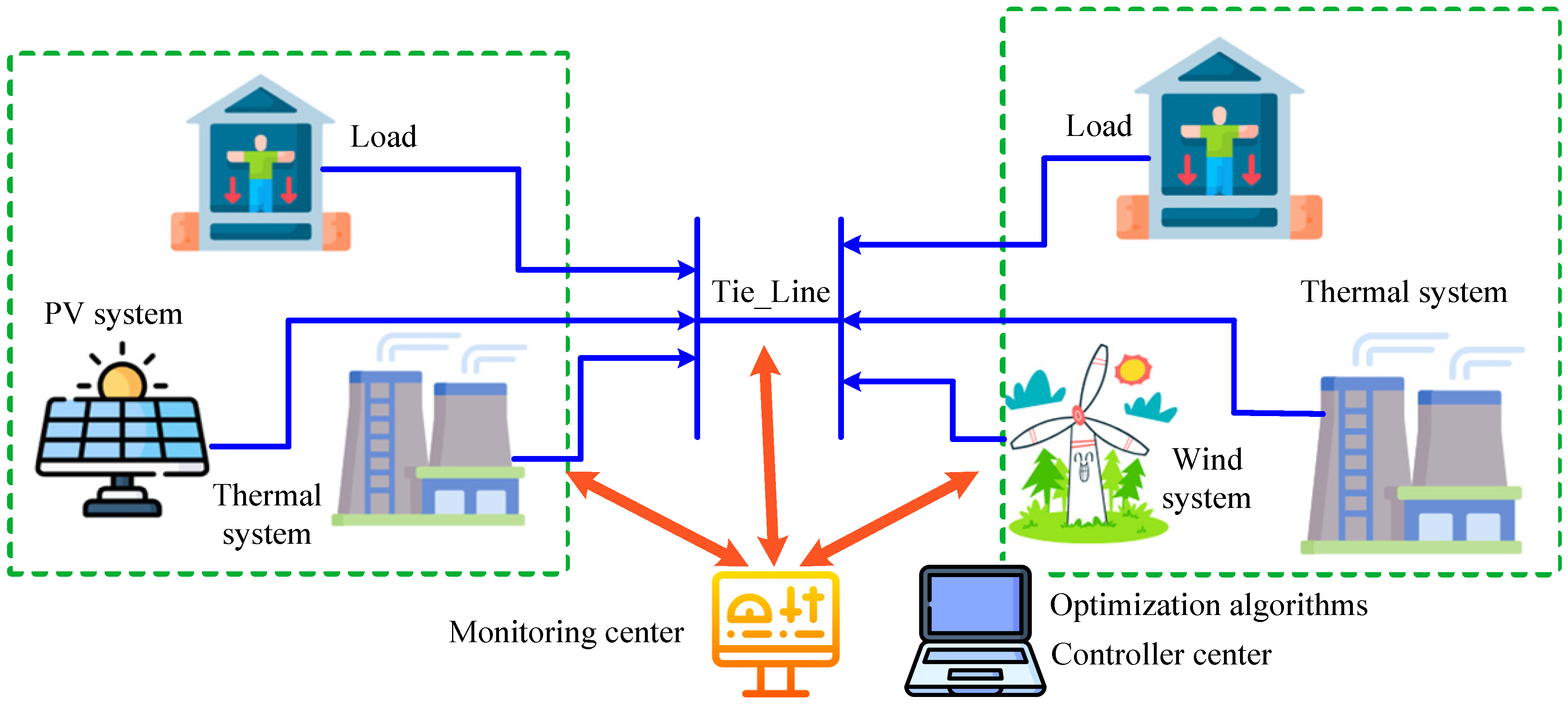Figure 1 displays the LFC structure of integrative power systems with RESs that this study proposes [13,14,15].

The oscillations in system operation, which can arise from factors like the integration of PV and WT plants into the electrical network or fluctuations in power demand, can be reduced by connecting parallel high-voltage direct current (HVDC) lines to the asynchronous current lines throughout the entire system [16]. In addition, elements such as an electron flow battery [17], a super capacitor [18], and a battery storage system [19] might increase the system’s efficiency.

Many industry and academic professionals use a variety of control strategies to accomplish load frequency management, which include conventional, soft-computing, and nature optimization techniques [20]. To decrease area control error (ACE) for optimal LFC process, several researchers have employed a range of conventional controllers, such as PID with diverse architectures (i.e., P, PI [21], ID [22], PD, PID [23]). Control professionals point out that simple ways of adjusting a PID controller may not be reliable. To achieve resilience, advanced control approaches [24] such as sliding mode (SM) control- and linear matrix inequality (LMI)-based methods are required. These controllers will outperform PIDs; however, it has been discovered that they increase the computing complexity and are insufficient for severe disturbances such as wind variations and abrupt load disturbances.

Numerous studies have explored various soft-computing approaches for optimizing PID controller gains to enhance power system performance. Commonly applied algorithms include particle swarm optimization (PSO) [25], ant colony optimization (ACO) [26], and the sine cosine algorithm (SCA) [27], which are widely recognized for their efficient search capabilities. Additionally, newer bio-inspired and nature-based methods such as the artificial rabbits algorithm (ARA) [28], bacterial foraging algorithm (BFA) [29], grasshopper optimization algorithm (GHO) [30], slap swarm algorithm (SSA) [17], and sooty terns optimization algorithm (STOA) [31] have shown promising results in nonlinear dynamic systems. Other advanced optimizers like the chaos game optimizer (CGO) [32], imperialist competitive algorithm (ICA) [33], grey wolf optimizer (GWO) [34], and genetic algorithm (GA) [35] have also been employed to solve the complex, multi-dimensional parameter-tuning problem inherent in power system LFC.

Parallel to the evolution of optimization techniques, significant attention has been paid to improving the structure and functionality of PID controllers themselves. Classical PID controllers have been extended into more sophisticated forms to offer better robustness, disturbance rejection, and adaptability in the presence of renewable energy fluctuations. These include cascade configurations such as the (1+PD)-PID [36], PI(1+DD) [13], PDF+(I+PI) [37], and PD-PIDN [38], which are tailored to mitigate overshoots and improve the dynamic response under varying conditions. Furthermore, fractional-order control schemes such as the fractional-order proportional-integral (FOPI) [38], fractional-order proportional-derivative (FOPD) [33], and fractional-order PID (FOPID) controllers [39,40] provide an additional degree of freedom in tuning, allowing for the more accurate modeling of real-world system dynamics. Hybrid structures like FOPID+FOPI [41], and combinations with tilt integral derivative (TID) controllers [42] have also emerged as powerful alternatives to classical control schemes.

In [43,44], the fractional and multilevel controller architecture was used to achieve LFC in a power system. In [45], to control the LFC of the connected electrical system of several areas including RESs, an ANFIS and an ant lion optimizer (ALO) are employed. Kushwaha et al. [46] and Nema et al. [47] examined the effects of combining a limited electric vehicle with quick responses to frequency into a power supply with low inertia, focusing on its techno-economic characteristics. In [48], a literature study on load frequency management was conducted on renewable energy sources incorporated into current power systems. The article discussed future trends and problems for various power system frameworks using HVDC connections, ESS, FACTS devices, and LFC-combined microgrids. In [21], the combination of PV panels into one of two power system components was the main focus of the investigation in several circumstances; the researcher assessed the impact of PV on both domains covered in [49,50].

Among the most sophisticated soft-computing techniques are algorithm-specific factors, and tweaking these settings takes longer than solving the issue itself. Current optimization strategies confront the following challenges:

• Optimization techniques might be traditional or intellectual system-based.
• The drawbacks of conventional approaches include the need for a close initial estimation and derivatives of the desired function and restrictions.
• The technique performance is largely dependent on certain parameters that must be modified to achieve global or close to the global optimums.
• Integrating various techniques into a hybrid technique boosts calculation time and makes tweaking more difficult, especially when method-specific factors are included.

Learning from previous research, the authors are motivated to apply the recently developed catch fish algorithm (CFA), which does not have certain method-specific variables, to enhance the efficiency of two-area LFC including integrated renewables. Taking CFA into consideration has the following advantages:

• Integration of CFA for LFC Optimization: This work introduces the application of the CFA, a recent nature-inspired metaheuristic for tuning the control parameters in LFC. CFA possesses distinct advantages, including its ability to maintain a balance between global exploration and local exploitation, faster convergence, and independence from problem-specific algorithm parameters. Its capability to reach global or near-global optima with minimal computational overhead makes it a robust and efficient tool for control optimization in power systems.
• Proposal of Multiple Advanced PID-Based Controllers for RES-Integrated Systems: This study suggests the implementation of a variety of advanced controllers, namely PI, PID, fractional-order PID (FOPID), PI with derivative and delay [PI(1+DD)], and cascaded PI [PI(PDN)] for enhancing the dynamic frequency response of a two-area interconnected non-reheat thermal power system integrated with renewable energy sources such as PV and wind power. This diversification of controller types under a unified optimization framework is novel in the context of renewable-based LFC.
• First-Time Application of CFA to Optimize Diverse Controller Structures: To the best of our knowledge, this is the first study to use CFA to optimize such a diverse set of controller architectures in a renewable-integrated LFC setting. Each controller’s gain parameters are tuned using the CFA based on performance indices like the IAE and ITAE, ensuring high precision in frequency regulation.
• Evaluation Under Multiple Realistic Operating Scenarios: The robustness and adaptability of the proposed controllers are thoroughly evaluated under a wide range of practical operating conditions, including step and random load disturbances, as well as both regular and irregular variations in solar and wind generation. This comprehensive analysis strengthens the practical relevance of this work for modern grid environments with high renewable penetration.
• Comparative Performance Assessment Against State-of-the-Art Algorithms: The proposed CFA-tuned controllers are benchmarked against well-established optimization techniques, including particle swarm optimization (PSO), brown bear algorithm (BBA), sine cosine algorithm (SCA), and grey wolf optimizer (GWO). The results confirm that CFA outperforms these techniques in terms of convergence speed, control accuracy, and system stability, thereby validating its suitability for complex power system applications.

The remainder of this paper is structured into the following sections: Section 2 provides an explanation of the elements that make up the power system utilized in this study. Details of the suggested controller are provided in Section 3. Section 4 introduces the optimization strategies utilized for LFC. In Section 5, the simulation findings are displayed, and in Section 6, the research is concluded.

2. Dynamic Model of Proposed System

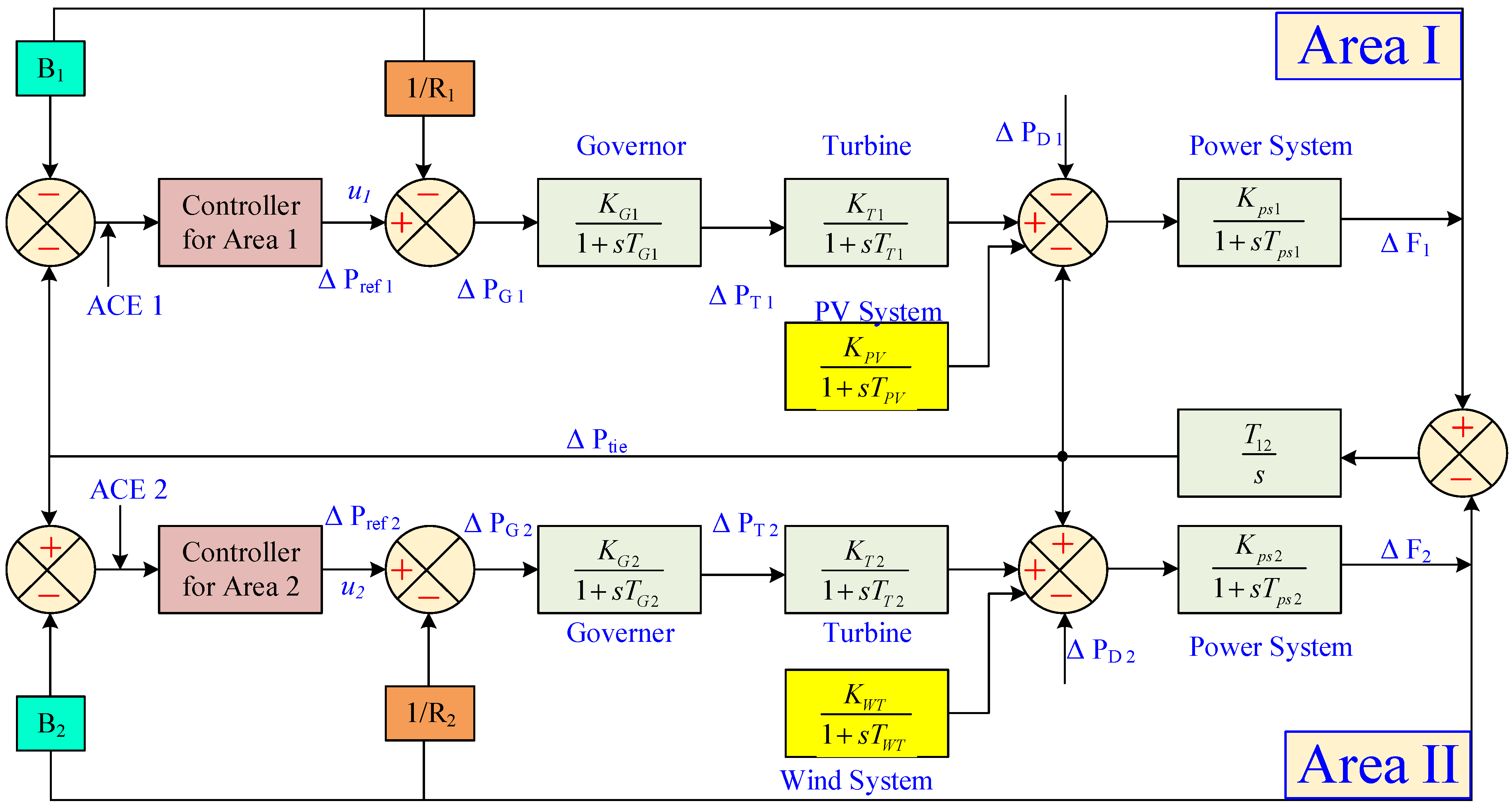
The proposed two-area non-reheat steam-powered system was modeled using the MATLAB/Simulink program (R2024b). Figure 2 shows the main elements of this framework. Area I consist of a solar system, load, and a non-reheat steam-powered facility. A wind turbine is combined with a non-reheat steam-powered facility in Area II. A controller is installed in every section of the power system. In order to make this study in the frequency domain simpler, every element of the system is modeled using first-order transfer functions. The subsequent figure provides a representation of the transfer function of the WT, photovoltaic, generator, and controlling systems [11,13].

Governor Model: This transfer function, G_G(s), represents the response of the governor system, which controls the input to the turbine to regulate system frequency. It is defined by the gain K_G and the time constant T_G as in Equation (1) [51,52]:

$$G_G(s)={\displaystyle \frac{K_G}{s{T}_G+1}}={\displaystyle \frac{1}{0.08 s+1}}$$

(1)

Turbine Model: The turbine model, represented by G_T(s), describes how the turbine reacts to changes in control input from the governor. It has a gain K_T and a time constant T_T, influencing the speed at which the turbine reaches steady-state as in Equation (2):

$$G_G(s)={\displaystyle \frac{K_T}{s{T}_T+1}}={\displaystyle \frac{1}{0.3 s+1}}$$

(2)

Power System Model: The power system model, G_PS(s), depicts the connection between power output and frequency in the system. Key parameters include K_PS, a proportionality constant, and T_PS, a time constant, which depends on system inertia H, frequency f, and load frequency dependency parameter D as in Equation (3):

$$G_G(s)={\displaystyle \frac{K_{PS}}{s{T}_{PS}+1}}={\displaystyle \frac{120}{20 s+1}}$$

(3)

where $K_{PS}={\displaystyle \frac{1}{D}},T_{PS}={\displaystyle \frac{2H}{Df}}$.

Load Frequency Dependency Parameter (D): D represents the sensitivity of the load to frequency changes, calculated as the ratio of nominal load P_l to nominal frequency f as in Equation (4):

$$D={\displaystyle \frac{\mathrm{Nominal} \mathrm{Load} (P_l)}{\mathrm{Nominal} \mathrm{Frequency} (f)}}$$

(4)

Solar power model: In this scenario, a solar power system may be denoted via a first-order transfer function, and Equation (5) shows that under the assumption of an unchanged ambient temperature, the PV plant’s output power shows a linear relationship with solar intensity.

$$G_{PV}(s)={\displaystyle \frac{K_{PV}}{s{T}_{PV}+1}}={\displaystyle \frac{1}{1.3 s+1}}$$

(5)

The wind turbine generation (W_TG) framework: Equation (6) describes the first-order transfer function framework for W_TG.

$$G_{PV}(s)={\displaystyle \frac{K_{WT}}{s{T}_{WT}+1}}={\displaystyle \frac{1}{1.5 s+1}}$$

(6)

Equations (7) and (8) calculate the ACE estimates for each area.

$$AC{E}_1=B_1\times \Delta F_1+\Delta P_{tie},$$

(7)

$$AC{E}_2=B_2\times \Delta F_2+\Delta P_{tie}$$

(8)

where the frequency bias parameters are B₁ and B₂.

The generator, power system, turbine, and PV plant time constants for area I are denoted by T_G1, T_T1, T_PS1, and T_PV in Figure 2, while the generator, turbine, power system, and WT time constants for area II are denoted by T_G2, T_T2, T_PS2, and T_WT. The generator, turbine, power system, and PV system gains of area I are represented by K_G1, K_T1, K_PS1, and K_PV, while the generator, power system, turbine, and WT gain in area II are represented by K_G2, K_T2, K_PS2, and K_WT. The frequency fluctuation in Hz is represented by ΔF₁ and ΔF₂, while the tie-line power fluctuation in p.u. is signified by ΔP_tie.

3. Proposed Controller Design

The main objective of load frequency control is to rapidly re-establish the nominal values of the system’s standard frequency and load variance across control regions when they are altered by further interruptions or changes in load. To address this issue, optimize peaking overshoot (+ve), peaking overshoot (−ve), and settling time (ts) should be improved. To address frequency deviations and enhance power system stability and reliability, four advanced control strategies are proposed and implemented in this study. These controllers aim to ensure consistent and accurate LFC performance under various operating conditions. The investigated controllers include the following:

• Classical PID Controller—a widely used baseline controller for LFC.
• PI(1+DD) Controller—an improved PI controller with a derivative-dominant compensator.
• PI(PDN) Controller—a cascaded PI controller designed to enhance disturbance rejection.
• Fractional-Order PID (FOPID) Controller—an advanced version of the PID controller with enhanced tuning flexibility using fractional calculus.

3.1. Classical PID Controller

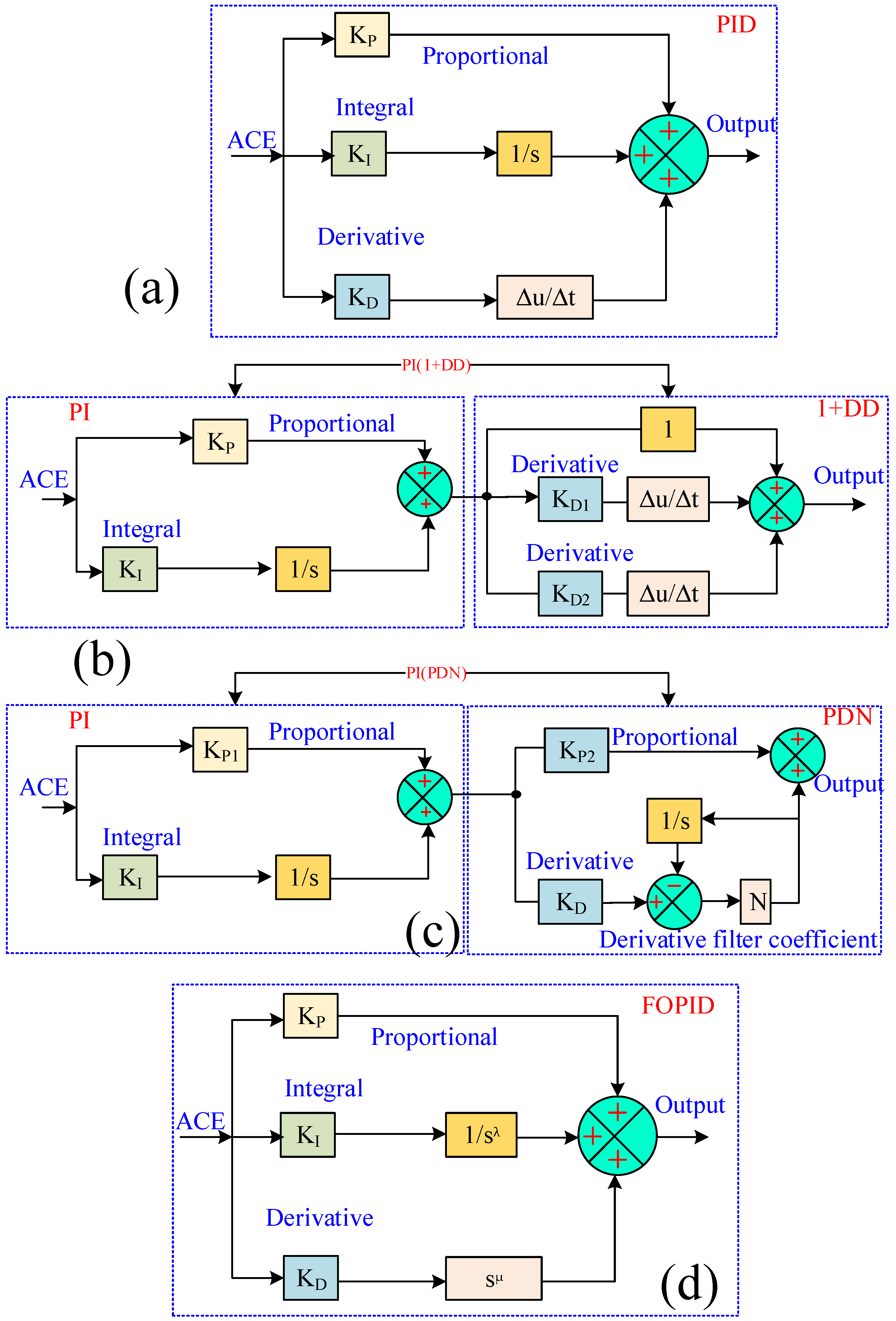
As seen in Figure 3a, a traditional PID controller has a straightforward structure, is reliable, and has a good effectiveness/cost-effectiveness ratio. It is more relevant in the engineering industry and requires less customer capabilities. PID controllers are useful for enhancing a system’s transient reaction through decreasing overshoot and settling time. The power grid’s overall stability and reliability are significantly increased when load frequency management is implemented using a PID control system.

Equation (9) is utilized to describe the PID controller’s transfer function.

$$G_{PID}(s)=K_P+{\displaystyle \frac{K_I}{s}}+s{K}_D$$

(9)

where K_P, K_I, and K_D are the PID control parameters.

The controllers of various ACEs (for i = 1, 2) receive impulses as input of the error, which are represented as Equation (10):

$$e_i(t)=AC{E}_i=B_i\Delta f_i+\Delta P_{tie}$$

(10)

According to Equation (11), the output of the power method’s controller for the erroneous input e_i(t) is u_i(t), where i = 1, 2.

$$u_i(t)=K_{Pi}\cdot e_i(t)+K_{Ii}{\displaystyle \int e_i(t)+}{K}_{Di}{\displaystyle \frac{d{e}_i(t)}{dt}}$$

(11)

3.2. Cascaded PI(1+DD) Control

The fundamental purpose of LFC is to reduce differences in system frequency and load fluctuations throughout control areas to conventional levels as rapidly as possible. To achieve this purpose, values including maximum and minimum overshoot, as well as settling duration, must be improved. Therefore, an extra control mechanism is essential for the more effective regulation of frequency fluctuations. To manage frequency variations, this work presents a controller named PI(1+DD) that outperforms traditional PID controllers.

Figure 3b shows the fundamental construction of the PI(1+DD) framework. As seen in the diagram, the framework controller has two levels: PI and DD. Additionally, the PI(1+DD) framework includes five different adjusting variables: a constant gain of 1 and four configurable controller gains (K_P, K_I, K_D1, and K_D2). The controller design is more flexible with these gain settings. The suggested PI(1+DD)) framework has the advantages of increasing the power system stability via lowering peak deviation and improving transient responsiveness, while the classical PID controller is ineffective during transient operation. The suggested controller’s transfer function is described in Equation (12):

$$G_{PI(1+DD)}(s)=\left(K_P+{\displaystyle \frac{K_I}{s}}\right)\times \left(1+s{K}_{D1}+s{K}_{D2}\right)$$

(12)

The proposed CFA method utilizes the integral of absolute error (IAE) of frequency deviations in both areas and tie-line power fluctuations as the objective function that will be applied in this work to maximize the controller gains. Consequently, Equation (13) provides the IAE objective function.

$$J_{obj}={\displaystyle \underset{0}{\overset{\infty }{\int }}\left(\left|\Delta F_1\right|+\left|\Delta F_2\right|+\left|\Delta P_{tie}\right|\right)}dt$$

(13)

The optimization problem, with bounds ranging from [−0.5, 0.5], is solved under the following constraints as Equation (14).

$$\begin{array}{l}{K}_{P(i-\min )}\le K_P\le K_{P(i-\max )},\\ K_{I(i-\min )}\le K_I\le K_{I(i-\max )},\\ K_{D1(i-\min )}\le K_{D1}\le K_{D1(i-\max )},\\ K_{D2(i-\min )}\le K_{D2}\le K_{D2(i-\max )}\end{array}$$

(14)

3.3. Cascaded PI(PDN) Controller

However, when faced with severe disturbances such as wind variations or unexpected load disturbances, the standard PID controller’s control capabilities are insufficient. To address these issues, numerous researchers have employed various strategies based on optimization techniques. These optimization strategies solve technical problems like nonlinearities, uncertainty, complexity, and resilience by optimizing the controller settings.

The literature uses modified PID control structures, including fraction-order and cascaded configurations of PID control, to further enhance the LFC effectiveness of the power system. Instead of using integers, the fractional-order PID controller (FOPID) uses fractional numbers for the proportional P, integral I, and derivative D, order of the control components. Comparing FO, cascaded, and intellectual controllers to traditional PID controllers, the former will improve performance and offer quicker disturbance rejection.

To boost the power system’s frequency stability, we used the recently created brown bear optimization method in this study to examine cascaded PI(PDN) controllers. Figure 3c depicts the proposed cascaded PI(PDN), which is a hybrid of dual controllers. The PDN controller uses the PI controller’s output as its input set point. It is possible to successfully manage supply and internal disruptions using this dual-stage control method. To keep disruptions from impacting other areas of the plant, the controller rejects them early. System performance is affected by the PID controller’s derivative filter coefficient (N). The control action’s fluidity is determined by this coefficient, which can improve control performance.

The cascade of the proposed PI(PDN) control and the transfer function is explained in detail in [53] using Equations (15) and (16).

$$C_1(s)=K_P+{\displaystyle \frac{K_I}{s}},$$

(15)

$$C_2(s)=K_P+K_D{\displaystyle \frac{N}{\frac{1}{s}N+1}}$$

(16)

where C₁(s) and C₂(s) refer to PI and PDN controllers, respectively. Consequently, Equation (13) provides the IAE objective function of the proposed PI(PDN) control.

There are limits on the gains of both PID and PI (PDN) controllers. Utilizing the following optimization problem, where i is the area number (i = 1, 2), the gains for PID and PI(PDN) controllers are determined. Reduce the objective function to a minimum = J being exposed in Equation (17):

$$\begin{array}{l}{K}_{P(i-\min )}\le K_P\le K_{P(i-\max )},\\ K_{I(i-\min )}\le K_I\le K_{I(i-\max )},\\ K_{D(i-\min )}\le K_D\le K_{D(i-\max )},\\ N_{(i-\min )}\le N_i\le N_{(i-\max )}\end{array}$$

(17)

After several trial runs, the controller’s gains minimum and maximum limits were determined to be −0.5 and 0.5, respectively. In the same way, the derivative filter coefficient has a range of 30 to 50.

3.4. Fractional-Order PID (FOPID) Controller

The FOPID controllers are a powerful expansion of the standard PID control framework that incorporates non-integer ordering for the proportional, integral, and derivative elements. This expansion increases the controller’s degrees of equality, allowing it to manage complicated systems with nonlinear dynamics, time delays, or non-integer order dynamics. FOPID controls, compared to their integer-order different forms, display non-local dynamics, requiring the use of the system’s error signal history to determine control action. FOPID is becoming common because of its resilience and superior performance [54]. The controller gain may be expressed as Equation (18), and its block structure is shown in Figure 3d.

$$G_{FOPID}(s)=K_P+K_I{\displaystyle \frac{1}{s^{\lambda }}}+K_D{s}^{\mu }$$

(18)

The FOPID controller’s transfer function is denoted by G, whereas λ and μ represent the fractional parts of the integral and derivative controllers, with corresponding gains of K_I and K_P, respectively. Furthermore, K_D represents the proportionate gain. In LFC, this error is frequently abbreviated as ACE. For the FOPID controller, ITAE is employed as the objective function to be reduced using the optimization approaches described in Equation (19).

$$ITAE={\displaystyle \underset{0}{\overset{t_{sim}}{\int }}\left(\left|\Delta F_1\right|+\left|\Delta F_2\right|+\left|\Delta P_{tie}\right|\right).t. }dt$$

(19)

4. Optimization Algorithms

The catch fish optimization method (CFA) is an optimization approach used in this research to schedule the gain in PI, PID, PI(1+DD), FOPID, and PI(PDN) controller gains for the two-area LFC integrated with RES. The main advantages of employing CFA are its computing efficiency and lack of algorithm-specific variables. The outcomes are compared with those of additional well-known metaheuristic algorithms, such as PSO, SCA, GWO, and BBA. The main advantages of utilizing the GWO and BBA algorithms for comparison are their simplicity, lack of computational complexity, and requirements for no particular input parameters. The primary advantage of employing the PSO and SCA algorithms is that their prospective solutions are accelerated through hyperspace, leading to a quicker advance towards better or ideal results. This idea is easy enough to implement using basic computer code, needing little memory and providing quick processing speed. The authors encourage the implementation of the aforementioned three optimization strategies for gain scheduling of the PI, PID, PI(1+DD), FOPID, and PI(PDN) controllers because of their advantages.

4.1. Proposed CFA

This study suggested that CFA was motivated by the traditional and straightforward fishing method. After examining the conceptual foundations of CFA, we will go over the key procedures that compose the algorithm [55,56].

In summary, the CFA is implemented in two phases: the exploration phase, which comprises cooperative fishing and dispersed exploration for advantages, and the exploitation stage, which involves coordinated encirclement efforts to capitalize on collective power [55]. The metaheuristic technique evaluates the global situation and ultimately decides on the best course of action by using search agents to provide continuous location updates. Equation (20) represents the CFA model, in which every fisherman acts as a search agent:

$$Fisher=\left[\begin{array}{cccc}{Fisher}_{1,1}& {Fisher}_{1,2}& \dots & {Fisher}_{1,d}\\ {Fisher}_{2,1}& {Fisher}_{2,2}& ⋮& {Fisher}_{2,d}\\ ⋮& ⋮& \ddots & ⋮\\ {Fisher}_{1,1}& {Fisher}_{1,2}& \dots & {Fisher}_{1,d}\end{array}\right]N\times d$$

(20)

Equation (21) is the resetting formulation of Fisher, which is a full matrix that contains the locations of N search agents in a d-dimensional space:

$$Fishe{r}_{i,j}=(u{b}_j-l{b}_j)\ast r+l{b}_j$$

(21)

The upper and lower bounds of the j-th dimension are represented by the variables ub_j and lb_j, the location of the i-th fisherman in the j-th dimension is represented by Fisher_i,j, and r is a random number between 0 and 1.

The fitness value assessment function f_obj and the current location data of each fisherman are used to calculate their fitness values. Equation (22) is the fitness value matrix that results from this.

$$fit=f_{objective}(Fisher)=\left[\begin{array}{c}{fit}_1\\ {fit}_2\\ ⋮\\ {fit}_N\end{array}\right]$$

(22)

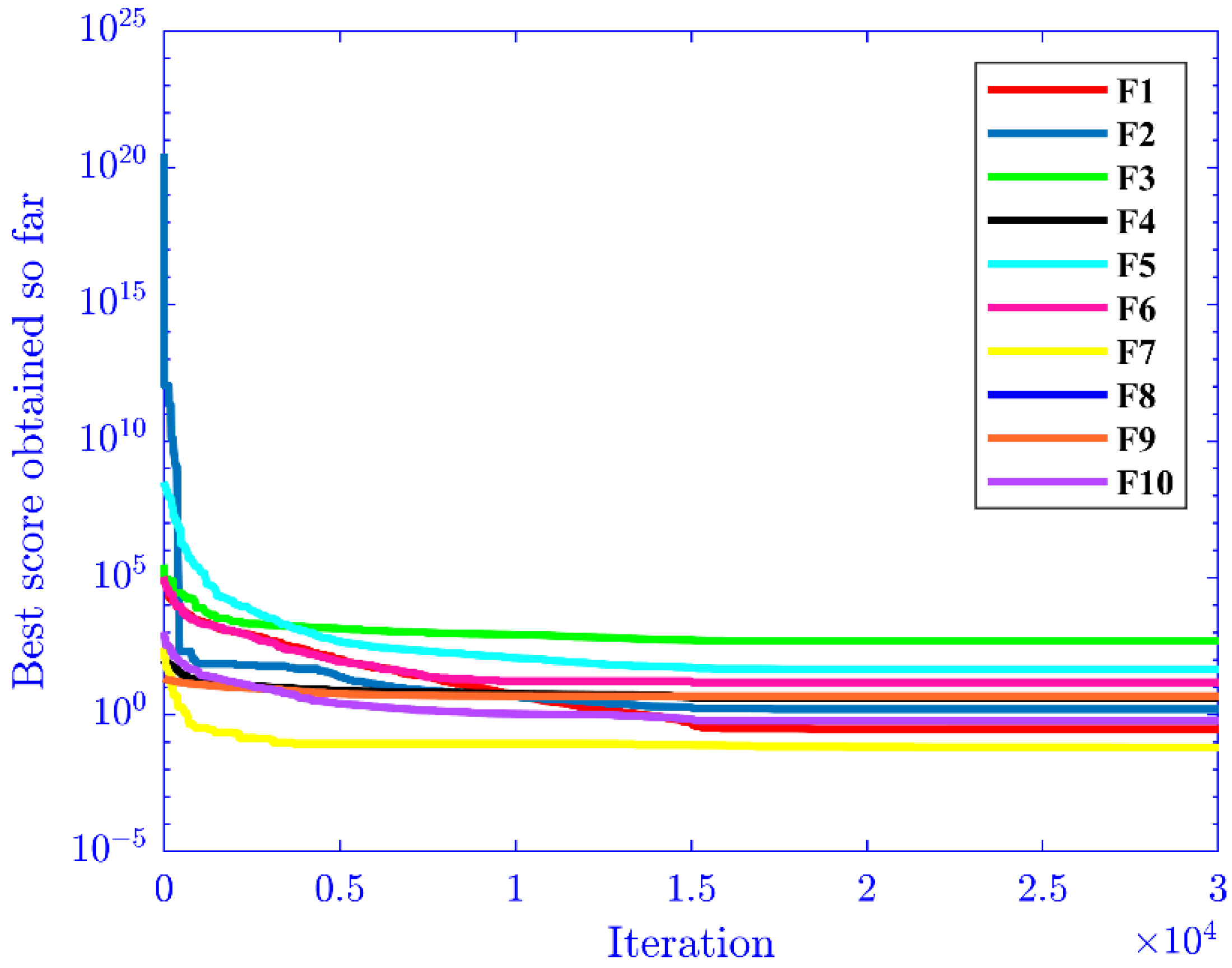
In the fitness matrix, fit₁ represents the first fisherman’s fitness value, fit₂ represents the second fisherman’s, and so on. The CFA convergence curves for ten common test functions are displayed in Figure 4. During the iterations, the algorithm employs 0.5 to split the fraction of exploration and exploitation. In the process, it is used in the second half of the phase (when EFs/MaxEFs ≥ 0.5) after the global has been studied in the first half (when EFs/MaxEFs < 0.5).

4.1.1. Exploration Phase (EFs/MaxEFs < 0.5)

The greatest capture rate and greatest quantity of fish were seen early in the fishing season; however, as the amount of fish that fishermen were able to catch progressively declined, so did the catch rate. Consequently, group encirclement is used as a backup search strategy while fishermen first concentrate on individually seeking and disruption of the water to gain a benefit. During the course of the hunt, the fisherman progressively gains the environmental edge over the fish. A rise in water turbulence and a fall in fish discernibility are the characteristics of this transition. The fish population falls and catch rates decline as a result of ongoing fish capture during the search. When collective encirclement becomes the primary means of survival, individual benefits become secondary to the needs of the group for which fishermen are suited. The parameter α, which represents the capture rate, is used to replicate the pattern’s transition as Equation (23).

$$\alpha ={(1-{\displaystyle \frac{3\times E{F}_s}{2\times MaxE{F}_s}})}^{{\displaystyle \frac{3\times E{F}_s}{2\times MaxE{F}_s}}}$$

(23)

Evaluations are expressed as EF_s, the current evaluation count, and MaxEF_s, the maximum evaluation value.

The fishermen have the freedom to select either group capture or self-sufficient search; however, when their catch rate α is high, their capture tactics favors self-sufficient search, and when α reduces, they transition to group capture, which we model using arbitrary integers (0, 1). p is the probability, α random number between 0 and 1, and group capture is selected when p ≥ α. Independent search is selected when p < a.

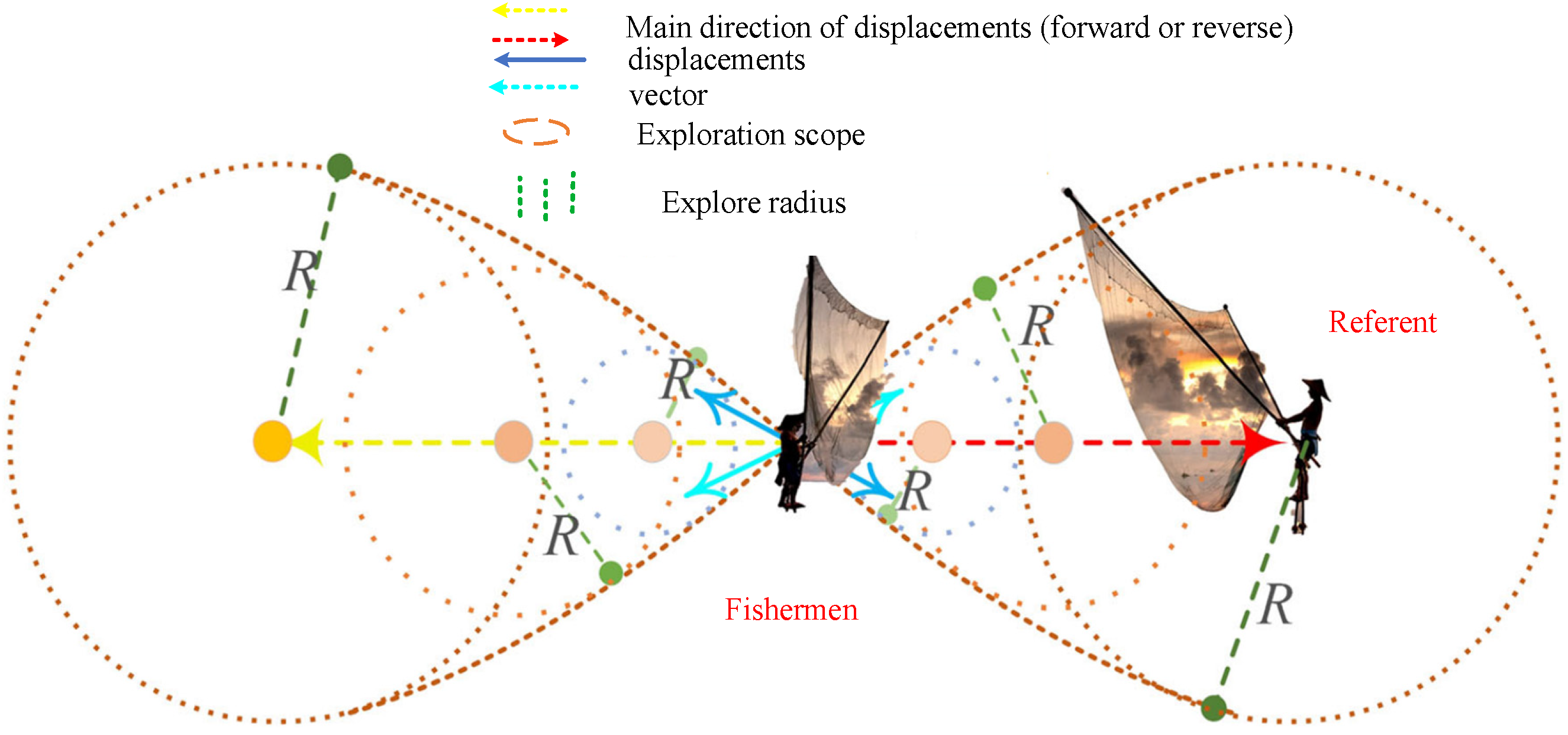
For independent search (p < a), Fishermen disturb the water to create a turbid environment, causing the fish to surface or release bubbles, which creates ripples. Based on these disturbances and capture success, fishermen adjust their search direction, focusing on local exploration or shifting to other areas as needed. The following is the update process illustrated in Equations (24)–(26):

$$Exp={\displaystyle \frac{fi{t}_1-fi{t}_p}{fi{t}_{\mathrm{maximum}}-fi{t}_{\mathrm{minimum}}}},$$

(24)

$$R=Dis\times \sqrt{\left|Exp\right|}\times (1-{\displaystyle \frac{E{F}_s}{MaxE{F}_s}}),$$

(25)

$$Fishe{r}_{i,j}^{T+1}=Fishe{r}_{i,j}^T+(Fishe{r}_{pos,j}^T-Fishe{r}_{i,j}^T)\times Exp+r_s\times s\times R.$$

(26)

One of these, Exp, has a range of values from (−1, 1) and is the significance of the empirical evaluation that the fisherman derived utilizing any posth (pos = 1 or 2 or… or N, p ≠ i) fishermen as the desire object. Following the Tth full position update, fit_max and fit_min represent the worst and best fitness scores, respectively. T is the number of times that the positions of the fisherman have changed. Following the repetitions of Tth and (T + 1)th, $Fishe{r}_{i,j}^T$ and $Fishe{r}_{i,j}^{T+1}$ reflect the location of the ith fishermen in j-dimension. The random number r_s is between 0 and 1. Dis represents the Euclidean separation between the referent and the ith person. A random unit vector of dimension d is denoted by s. Calculate the primary direction of movement (this particular person received the favorable instruction from the fishermen) and duration using statistical analysis. R is either lower or equal to Dis. Additionally, the number of evaluations (EFs) and the absolute quantity of Exp affect the exploration domain R that are currently conducted. The fisherman in the middle of Figure 5 is depicted as stretching both in the direction of and away from the reference point. The radius, which forms a stacked circular pattern and a brown exploring range, is defined as the distance between each point and the center. The fisherman in Figure 5 on the left is shown getting ready to move, while the randomly referenced fisherman is seen on the right. The fisherman’s flexibility in motion is indicated by the brown region, where R is the movement radius. The primary movement direction is indicated by the yellow and red arrows, while the independent search drift of the fisherman is depicted by the blue arrow.

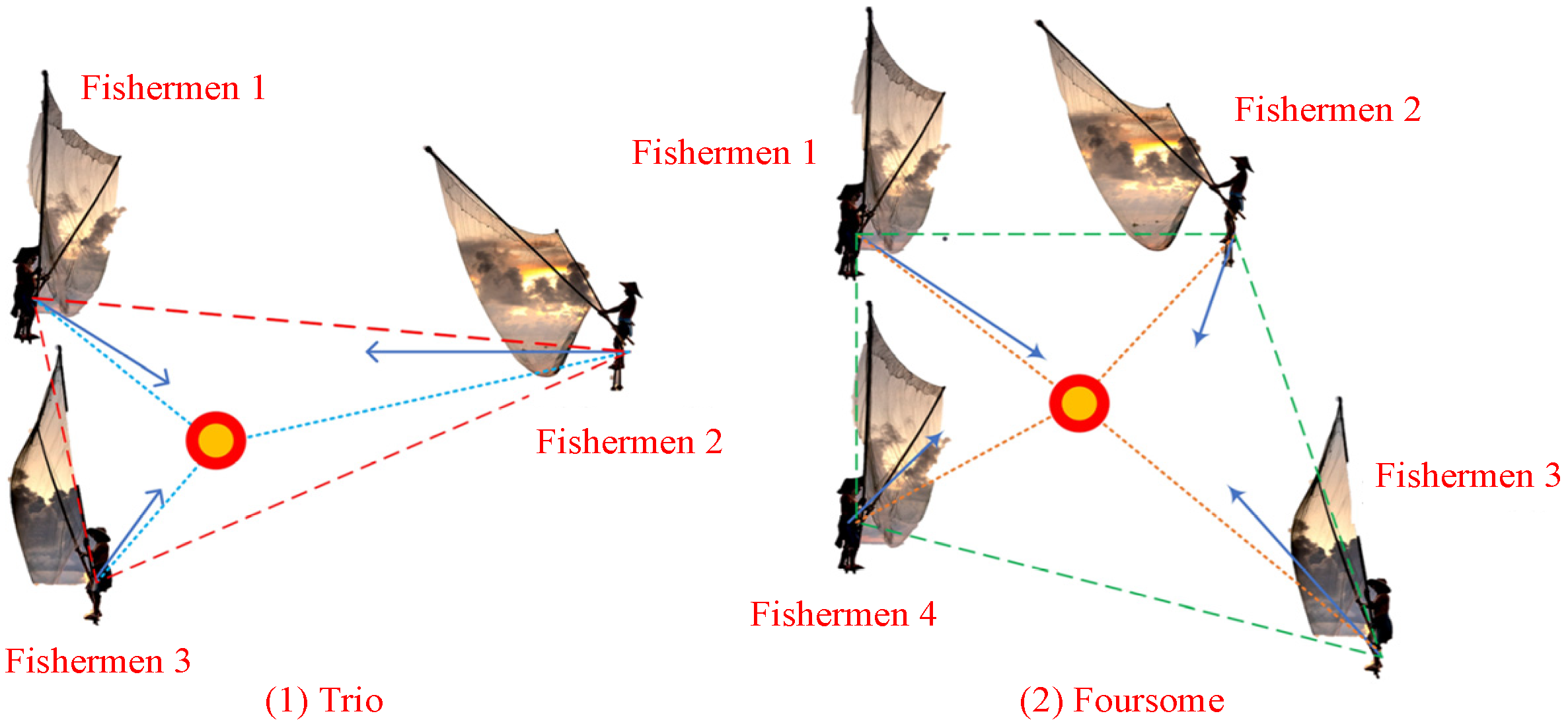
Fishermen work together in groups of three or four to surround possible fish spots for the group capture (p ≥ α), using nets to increase their catch. The environment, team relationships, and health all affect the direction and distance of their movements; as more fish are caught and people congregate, their motions become more accurate. Figure 6 displays the method’s schematic representation. The following is how the model and formula are developed as Equations (27) and (28):

$$Centr{e}_c=mean(Fishe{r}_c^T),$$

(27)

$$Fishe{r}_{c,i,j}^{T+1}=Fishe{r}_{c,i,j}^T+r_2(Centr{e}_c-Fishe{r}_{c,j}^T)+\left(1-{\displaystyle \frac{2\times E{F}_s}{MaxE{F}_s}}\right)\times r_3.$$

(28)

The c consists of three or four people whose places have not been changed. The red–orange point in Figure 6 is the Centre_c, the goal point for group c’s encirclement. Following the Tth and (T + 1)th, updates, $Fishe{r}_{c,i,j}^{T+1}$ and $Fishe{r}_{c,i,j}^T$ indicate the location of the ith fisherman in group c in the j-dimension. The fisherman’s pace as he reaches the center, or r₂, varies from person to person and can be anywhere between 0 and 1. The move offset, or r₃, has a value from [−1, 1], which progressively shrinks as the number of EFs rises. In Figure 6, the blue arrow represents the fisherman’s movement’s ultimate direction and distance in two dimensions.

4.1.2. Exploitation Phase (EFs/MaxEFs ≥ 0.5)

There are fish that escape throughout the fishing procedure, but fishermen work together to drive and surround them. Fishermen are positioned around the fish, with the center focusing on catching the main group and the outer ones targeting escapees. This cooperative strategy improves capture rates. The distribution follows a Gaussian model, as shown in Figure 7, with the updated Equations (29) and (30) below:

$$\sigma =\sqrt{\left(2\left(1-{\displaystyle \frac{E{F}_s}{MaxE{F}_s}}\right)/\left({\left(1-{\displaystyle \frac{E{F}_s}{MaxE{F}_s}}\right)}^2+1\right)\right)}.$$

(29)

$$Fishe{r}_i^{T+1}=G_{best}+GD\left(0,{\displaystyle \frac{r_4\times \sigma \times \left|(Fisher)-G_{best}\right|}{3}}\right)$$

(30)

These include GD, which is the Gaussian distribution functional. The general variance σ rises with the number of assessments reaching 0 from 1, while the general average µ stands at 0. The average value of every dimension in the middle of fishermen is a matrix of the ith fisherman’s location following the (T + 1)th iteration. Globally, the perfect spot (G_best) is represented by the red circle in Figure 7, and the fishermen are distributed in three ranges by r4, a random number with values of {1, 2, or 3}.

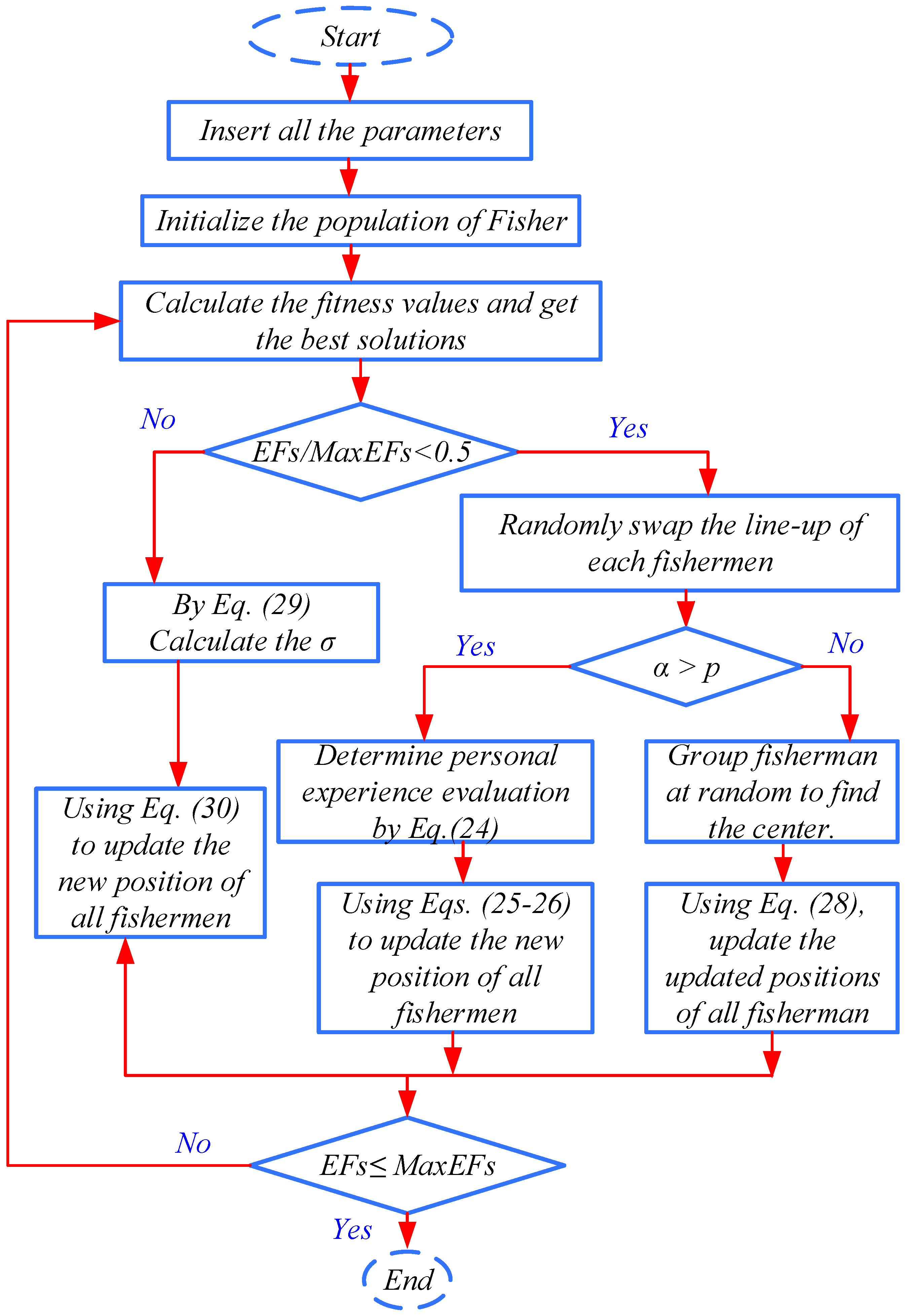
4.1.3. Implementation Process of CFA

The PSO search mechanism randomly chooses a separate region to evaluate and compare the exploration scenario, which is not the same as the independent search mode. If the two are comparable, it keeps exploring its own region; if it is better, it examines other places in reverse; and if it is worse, it goes to someone else. The local region is explored through encircling, and the individual search is transformed into a collective search based on the capture rate, enhancing the thoroughness and effectiveness of global exploration. In order for the algorithm to produce better results, the best position is lastly continually refined using collective capture. The CFA primarily places the emphasis on two phases of optimization: the exploration and exploitation phases. The procedure is depicted in the flowchart in Figure 8.

4.2. Grey Wolf Optimizer

The GWO is a population-specific heuristic technique developed by [57]. The GWO exclusively adheres to the grey wolf’s instinctive leadership and hunting tactics. Grey wolves are social animals that typically live in packs of five to twelve members, depending on the size of the group. The steps for addressing the optimization issue using GWO are described in [13].

4.3. Particle Swarm Optimizer

The PSO is an optimization approach that uses the mobility and intelligence of swarms to solve challenging optimization problems. In 1995, Eberhart and Kennedy presented the PSO approach based on the motivation for foraging and social behavior of fish schooling, bird flocking, and swarm theory. The steps for addressing the optimization issue using PSO are described in [58].

4.4. Brown Bear Optimizer Algorithm (BBA)

The brown bear optimizer (BBA) algorithm is a metaheuristic optimization technique inspired by the natural foraging behavior of brown bears. Like many swarm-based algorithms, BBA models the collective and strategic movement of brown bears in the wild as they search for food. These bears typically utilize a combination of exploration (searching broadly for new resources) and exploitation (focused searching once resources are identified) to optimize their foraging efficiency. The algorithm emulates this dual strategy, striking a balance between exploration and exploitation to effectively tackle complex, multidimensional optimization problems.

In BBA, the population of bears represents potential solutions, and their positions in the solution space are adjusted over iterations based on the best-known solutions (similar to other population-based optimizers like PSO and GA). By integrating these natural behaviors, BBA is adept at escaping the local optima and exploring a wider range of possible solutions, making it effective for diverse and challenging optimization tasks.

The brown bear optimizer is applied in fields such as machine learning, engineering design, and network optimization, where it provides robust, adaptable solutions to complex optimization problems. As demonstrated in [11], the optimization techniques are developed by mathematically modeling the two different behaviors of brown bears, pedal scent marking and sniffing.

4.5. Sine Cosine Algorithm (SCA)

Seyedali Mirjalili [1] developed the SCA to address optimization difficulties. The SCA is a mathematical optimization strategy that mimics the behavior of the sine and cosine functions in order to find the best solution. The SCA employs sine and cosine functions to update a set of random solutions, creating a new population. These functions adjust the solutions by either moving them closer to or further from the global best solution. Equations (31) and (32) were used to update the position, as follows:

$$X_i^{t+1}=X_i^t+{\alpha }_1\times \sin ({\alpha }_2)\times \left|{\alpha }_3{P}_i^t-X_i^t\right|$$

(31)

$$X_i^{t+1}=X_i^t+{\alpha }_1\times \cos ({\alpha }_2)\times \left|{\alpha }_3{P}_i^t-X_{ii}^t\right|$$

(32)

where X_i signifies the particle’s current location in the i-th dimension; α₁, α₂, and α₃ signify random values; and P_i specifies the destination point’s position in the same dimension. According to [1], the SCA algorithm outperforms other metaheuristic algorithms by a significant margin.

5. Simulation Results Analysis and Discussions

In this section, the simulation outcomes were used to assess the performance of the algorithms and proposed controllers. The MATLAB/Simulink program was used to study a two-area non-reheat thermal power system and the controllers PID, PI(1+DD), FOPID, and PI(PDN). Customers’ load demands might vary in size and value within power systems. As a result, the controllers and optimizer techniques to be employed for LFC should maintain the frequency of the system within the designated ranges in the face of all load demands of varying magnitudes. Furthermore, because RESs like WT and PV are variable and would be included in the power system when conventional energy sources are insufficient, it is critical that the utilized controllers and optimization techniques work well. Taking all of this into account, this study’s simulation looked at a few distinct scenarios depending on whether RESs were there or not and how the system’s load changed randomly.

To investigate the system’s responses, the gain in the PID, PI(1+DD), FOPID and PI(PDN) controllers for the studied systems is precisely adjusted using CFA for optimal tuning. To compare the performance of the system, a few different optimum tuning methods such as GWO, PSO, BBA, and SCA were used. A simulation experiment was conducted using the utilized approach. The results of these investigations are briefly discussed in the next section.

Table 1. The parameters of the considered two-area power system.

Parameter	Value	Parameter	Value
TPV	1.3 s	KPV	1 Hz/pu.MW
TWT	1.5 s	KWT	1 Hz/pu.MW
TPS	20 s	KPS	120 Hz/pu.MW
TT	0.3 s	KT	1 Hz/pu.MW
TG	0.08 s	KG	1 Hz/pu.MW
T1,2	0.545 pu.MW/Hz	a1,2	–1
R1, R2	2.4 Hz/pu.MW	B1, B2	0.425 pu.MW/Hz

shows the characteristics of the two-area power system under consideration.

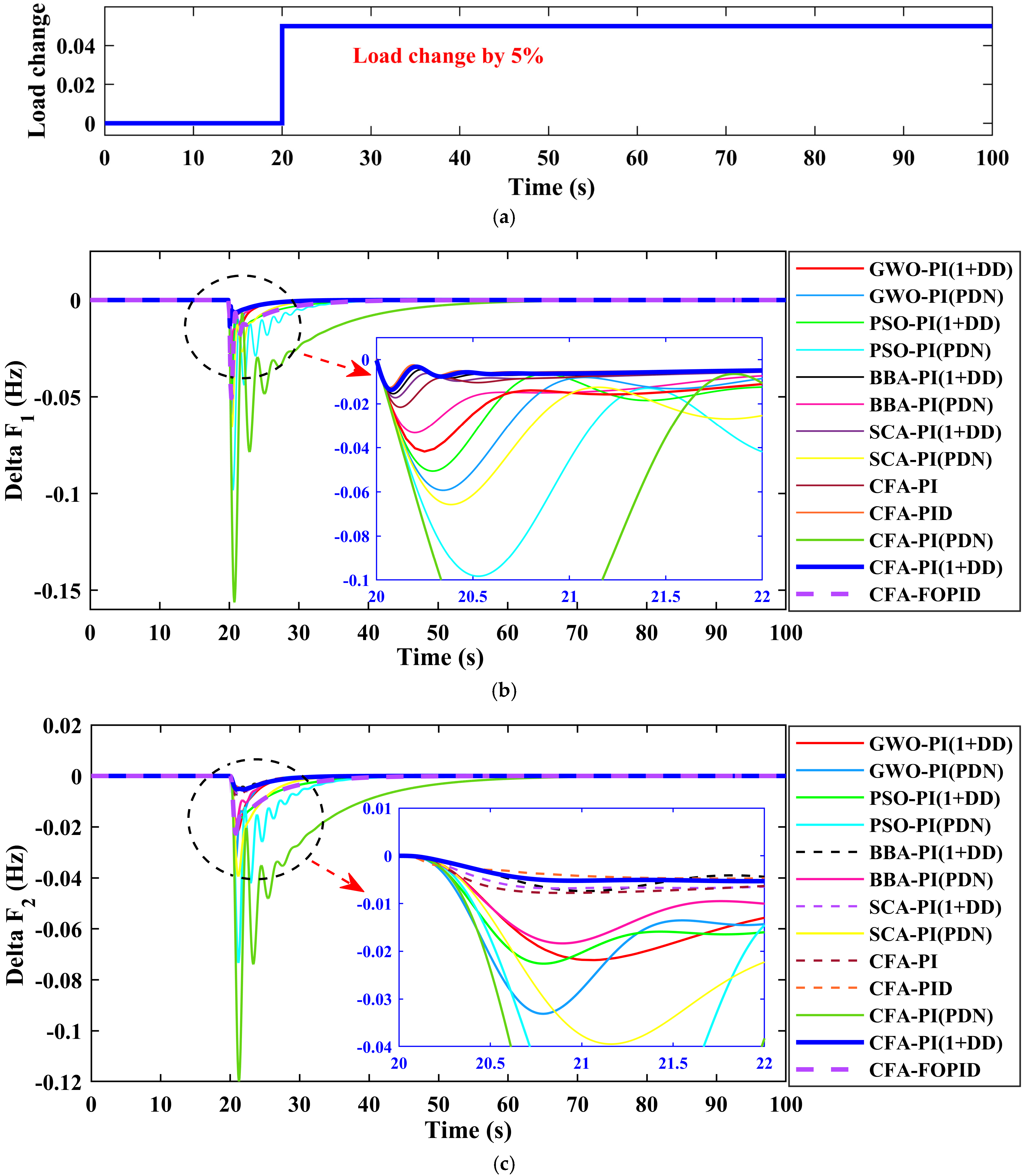
5.1. Case One: 5% Load Change at Area-1

The performance of many CFA-, BBA-, GWO-, SCA-, and PSO-tuned controllers, including PID, PI(1+DD), FOPID, and PI(PDN), was evaluated in this instance for a 5% load shift in Area 1 without RES production, as seen in Figure 9a. As a consequence of the simulations, Figure 9b–d display the frequency and tie-line power variances. In comparison to other controllers, as seen in Figure 9 and

Table 2. The system’s performance under a 5% load change.

Controller	Δf1 (Hz)			Δf2 (Hz)			ΔPtie (pu.MW)
	+ve	−ve	ts	+ve	−ve	ts	+ve	−ve	ts
GWO-PI (1+DD)	0.014	−0.015	21.5	0.003	−0.02	20.9	0.0049	−008	27.8
GWO-PI (PDN)	0.0062	−0.059	22.3	0.013	−0.033	20.7	0.006	−0.012	21.4
PSO-PI (1+DD)	0.0064	−0.050	29.1	0.0133	−0.022	34.4	0.06	−009	21.3
PSO-PI (PDN)	0.0013	−0.098	36.7	0.034	−0.067	39.2	0.01	−0.03	36.7
BBA-PI (1+DD)	0.0054	−0.017	20.7	0.0028	−0.0077	25.2	0.002	−0.001	20
BBA-PI (PDN)	0.015	−0.033	23.8	0.01	−0.02	24.3	0.0045	−0.0032	21.8
SCA-PI (1+DD)	0.007	−0.017	21.1	0.0045	−0.0077	33.7	0.007	−0.01	28.9
SCA-PI (PDN)	0.012	−0.066	35.8	0.004	−0.04	30.8	0.001	−0.001	20
CFA-PI	0.0076	−0.021	20.9	0.005	−0.0077	23.4	0.001	−0.001	20
CFA-PID	0.004	−0.013	20.1	0	−0.005	21.1	0	−0.001	20
CFA-PI (1+DD)	0.006	−0.16	55.6	0.01	−0.12	39.1	−0.01	−0.05	54.8
CFA-PI (PDN)	0.004	−0.013	20.1	0	−0.005	21.1	0	−0.001	20
CFA-FOPID	0.003	−0.14	44.6	0.01	−0.12	39.1	−0.01	−0.05	54.8

, the CFA-adjusted PID, PI(1+DD), FOPID, and PI(PDN) controllers yield superior outcomes in regards of the overshoot levels for the system frequency and tie-line power fluctuations as well as the settling time of these fluctuations as shown in Equations (33)–(35). The frequency fluctuations, tie-line power deviation, settling time (ts), and positive and negative peaking overshoot (+ve and −ve) for a 5% load shift in Area 1 are all shown in Table 2.

$$+ve=max(\Delta x(t))-\Delta x_{ss},$$

(33)

$$-ve=min(\Delta x(t))-\Delta x_{ss},$$

(34)

$$t_s=time when,\left|\Delta x(t)-\Delta x_{ss},\right|\le Tolerance for all(t)\ge t_s$$

(35)

where Δx(t), is the response variable (either ΔF1/ΔF2 or ΔPtie at time t. Δxss, is the steady-state value of the response variable (often zero for deviation variables in control systems). The Tolerance can be calculated based on the percentage of the steady-state value. For a 5% tolerance band: $Tolerance=0.05\times \left|\Delta x_{ss}\right|$, For systems where Δxss = 0, the tolerance is typically defined based on a percentage of the initial peak value of Δx.

The frequency variation (ΔF1) in Area 1 following a 5% load disturbance is displayed in Figure 9b. A distinct control strategy (PI-(PDN), PI-(1+DD), FOPID, and PID) adjusted by several optimization methods (BBA, SCA, GWO, PSO, and CFA) is shown by each line. The proposed CFA-based PI-(1+DD) controller, shown by the blue line, performs better than alternative techniques such as CFA-FOPID, CFA-PI-(PDN), CFA-PID, CFA-PI, and other controllers optimized by other techniques. In particular, the CFA-PI-(1+DD) exhibits a rapid reaction with less overshoot and a quicker settling time, successfully stabilizing the frequency deviation at zero. This behavior indicates that the proposed CFA-PI-(1+DD) controller in Area 1 is more capable of managing load disturbances. The frequency variation (ΔF2) in Area 2 after the same 5% load disturbance is shown in Figure 9c. Each curve represents a distinct control approach that has been adjusted by an optimization technique, much like in Figure 9b. Once more, the suggested CFA-PI-(1+DD) controller performs quite well, rapidly stabilizing the frequency deviation with no overshoot or oscillation. The figure’s inset, which focuses on the transient response, demonstrates how well CFA-PI-(1+DD) reduces deviations in comparison to other controllers. This suggests that in Area 2, CFA-PI-(1+DD) offers improved load frequency management.

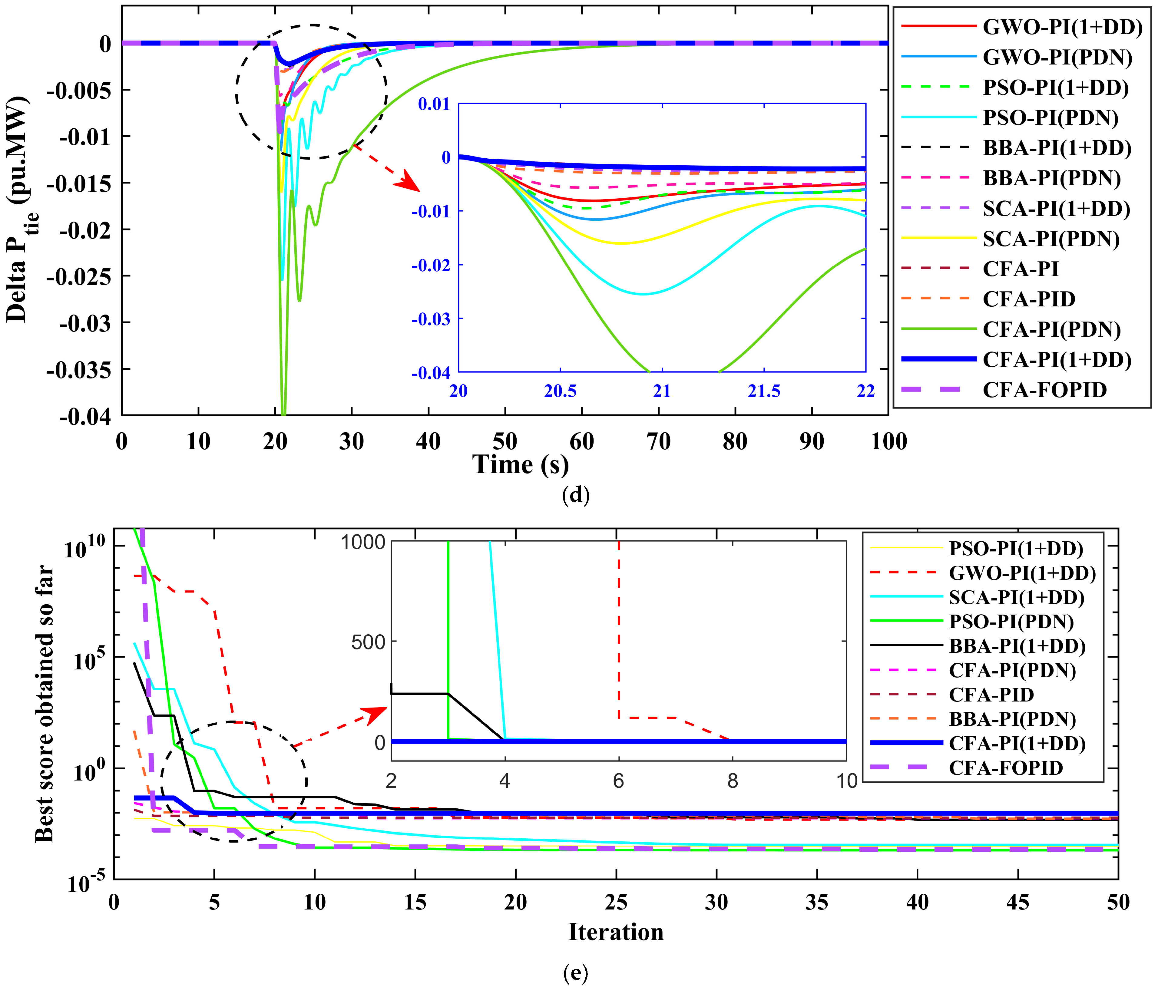
The tie-line power deviation (ΔPtie) between Areas 1 and 2 as a result of the load variation is shown in Figure 9d. Similar to the earlier representations, every line denotes a distinct control strategy. By effectively reducing the tie-line power variation and enabling the system to rapidly recover to its steady state, the CFA-PI-(1+DD) controller achieves the greatest performance. This figure’s inset, which focuses on the first response, shows that CFA-PI-(1+DD) lowers the power deviation more quickly and with fewer oscillations than alternative techniques such as CFA-FOPID, CFA-PI-(PDN), CFA-PID, CFA-PI and other controllers. Even with the incorporation of renewable energy, this performance is essential for preserving the power balance across interconnected areas and guaranteeing dependable system operation. The convergence performance of control strategies for a specific control strategy (PI-(PDN), FOPID PI-(1+DD), and PID) tuned by various optimization algorithms (PSO, GWO, SCA, BBA, and CFA) is shown in Figure 9e. The proposed CFA-PI-(1+DD) controller demonstrates the fastest and most consistent convergence, reaching a low error value within a few iterations and stabilizing quickly. This indicates that CFA-PI-(1+DD) requires fewer iterations to achieve optimal tuning, making it efficient in reaching a high-quality solution.

Table 1 illustrates how the traditional PI and PID controllers enhance the settling time in comparison to the PI(1+DD), FOPID, and PI(PDN) controllers. In contrast to the PID, FOPID, and PI(PDN) controllers, the suggested controller CFA-PI(1+DD) exhibits less oscillations in negative peak overshoot. Additionally, the positive peak overshoot is set to zero by the CFA-PI(1+DD) controller. As a consequence, the CFA-PI(1+DD) controller outperforms the PI, PID, FOPID, and PI(PDN) controllers. In conclusion, the CFA-PI-(1+DD) controller performs better than alternative control techniques such as CFA-FOPID, CFA-PI-(PDN), CFA-PID, CFA-PI, and other controllers across all figures due to its rapid stabilization, low overshoot, and strong reaction to load perturbations. For load frequency management in multi-area systems, this makes it extremely effective.

Table 3. CFA optimally tuned controller’s parameters.

Optimized Technique	Area One				Area Two
	KP	KI	KD1	KD2	KP	KI	KD1	KD2
CFA-PI-(1+DD)	−1	−1	−0.231	1	0.17156	−0.24906	−0.0232	−0.377
CFA-PI-(PDN)	0.8923	0.9994	0.1674	-	0.9937	0.9907	0.1068	-
CFA-FOPID	0.8627	5.2257	0.5146	-	5.6736	4.687	4.6986	-
CFA-PID	0.8925	0.9576	0.9664	-	0.8919	0.9978	0.1825	-
CFA-PI	0.0343	−0.7302	-	-	−0.6920	0.1635	-	-

For FOPID, the λ1 = 0.5100, μ1 = 0.5882, λ2 = 0.4612, μ2 = 0.9988.

displays the gain values of the controllers employed in the system as a result of the optimization process, which were established using case one.

5.2. Case Two: The Performance of Controllers at Different Step Load Perturbations

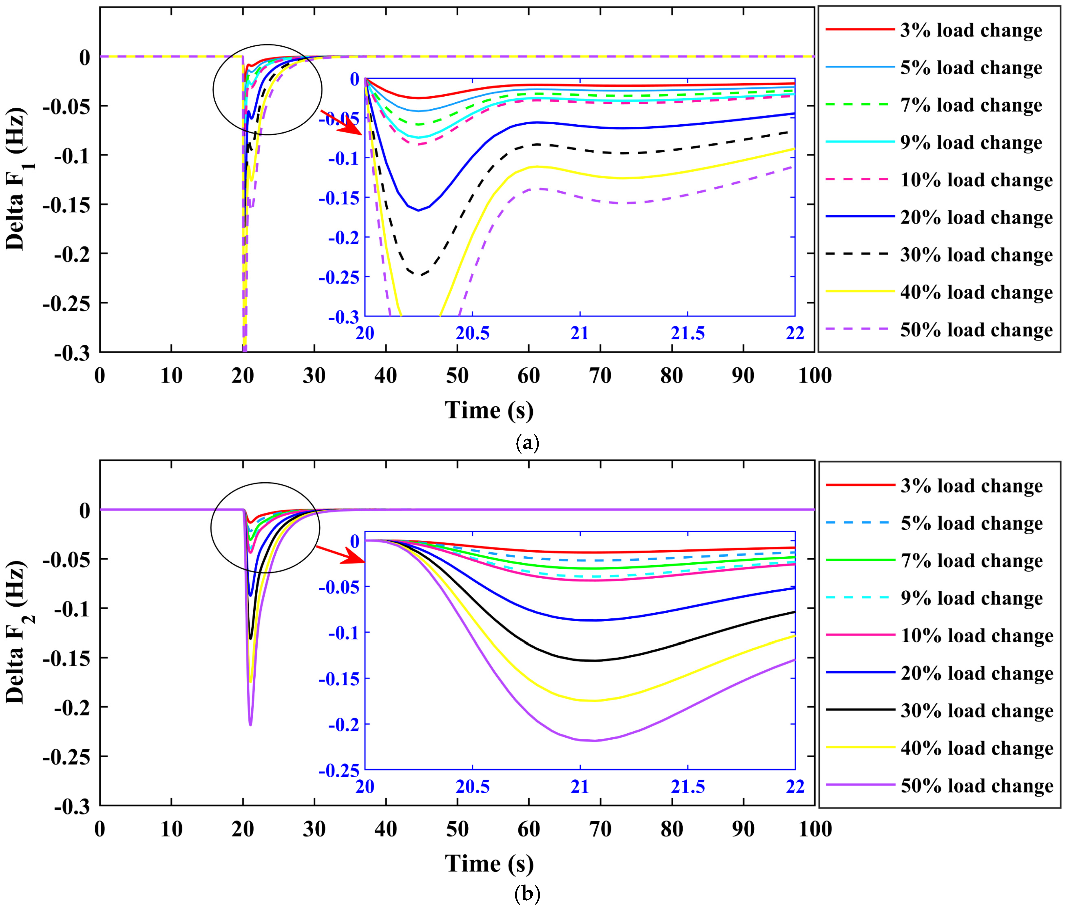
In order to demonstrate the usefulness of the suggested controller, and through the modification of the controller parameters found in Table 3, the behavior of the proposed CFA-PI-(1+DD) controller under various load demands was examined. In Figure 10, the system responses are displayed. Both the maximum and lowest overshoot values of the fluctuations rise as load changes do, as the figures demonstrate. Variations, however, fall within reasonable bounds.

Figure 10a shows the frequency deviation (ΔF1) in Area 1 at various load change percentages between 3% and 50%. Every line indicates a distinct value for the load change. There is a greater initial dip when the frequency deviation rises in tandem with the load disturbance. Effective damping is demonstrated by the suggested CFA-PI-(1+DD) controller at all load levels, with responses reverting to zero quite rapidly following the disturbance. A magnified view of the transient response is shown in the inset, which demonstrates how the controller maintains system stability even in the face of substantial disturbances (such as a 50% load shift), while longer settling periods are a natural consequence of greater disturbances.

The frequency deviation (ΔF2) in Area 2 for the same range of load variations is shown in Figure 10b. Larger frequency variations are caused by greater load shifts, much like in Area 1. With few oscillations and a distinct route to steady state, the suggested CFA-PI-(1+DD) controller efficiently stabilizes the response in every scenario. More information on the system’s transient behavior is provided in the inset, which also demonstrates how the controller can manage different disturbance levels while preserving reliable performance and settling very rapidly in all load change circumstances.

The tie-line power variation (ΔPtie) for various load fluctuations is displayed in Figure 10c. As anticipated, larger load variations result in larger tie-line power variances. By effectively mitigating these variations, the CFA-PI-(1+DD) controller guarantees that following a disturbance, the power exchange across regions recovers to its nominal value. The first reaction is the main emphasis of the inset, which shows that even with greater load fluctuations, the controller reduces oscillations and stabilizes tie-line power more quickly.

Across all subfigures in Figure 10, the CFA-PI-(1+DD) controller performs well under varying loads, with good damping, little overshoot, and speedy stabilization. This demonstrates the controller’s capacity to keep frequency and tie-line power stability in an interconnected system despite considerable load changes, guaranteeing resilience and efficiency in the presence of renewable energy sources.

5.3. Case Three: Random Load Fluctuations

Additionally, a random load fluctuation between 0.02 pu and 0.03 pu was applied for Area 1 in order to test the performance of the suggested controller under various disturbances. Figure 11a shows the system’s oscillations under the load adjustments. The results unequivocally show that the tie-line power and frequency variations happen during the times when the load varies. The results also indicate that compared to other controllers, the proposed controller yields the best performance in terms of system frequency overshoot, tie-line power fluctuation, and the settling time of these changes.

Figure 11b,c shows the frequency variation in Area 1 and Area 2 due to random load fluctuations. Each line indicates a separate control technique that has been optimized using several methods. When compared to existing controllers such as CFA-FOPID, CFA-PI-(PDN), CFA-PID, CFA-PI, and other controllers, the suggested CFA-PI-(1+DD) controller exhibits consistently low-frequency variations. The zoomed-out areas in Figure 11b,c show the CFA-PI-(1+DD) controller’s transient responses to specific disturbances, which show greater stability and rapid convergence, effectively dampening oscillations and swiftly reverting the frequency deviation to near-zero.

Figure 11d shows the tie-line power deviation (ΔPtie) between Areas 1 and 2 owing to random load changes. The CFA-PI-(1+DD) controller (in blue) successfully reduces tie-line power variations while maintaining balance between zones. The zoomed-out area in Figure 11d focus on transitory events, demonstrating the controller’s rapid responsiveness and low oscillations as compared to alternative techniques such as CFA-FOPID, CFA-PI-(PDN), CFA-PID, CFA-PI, and other controllers. This precise regulation of tie-line power is critical for assuring coordinated operation and stability throughout linked regions. 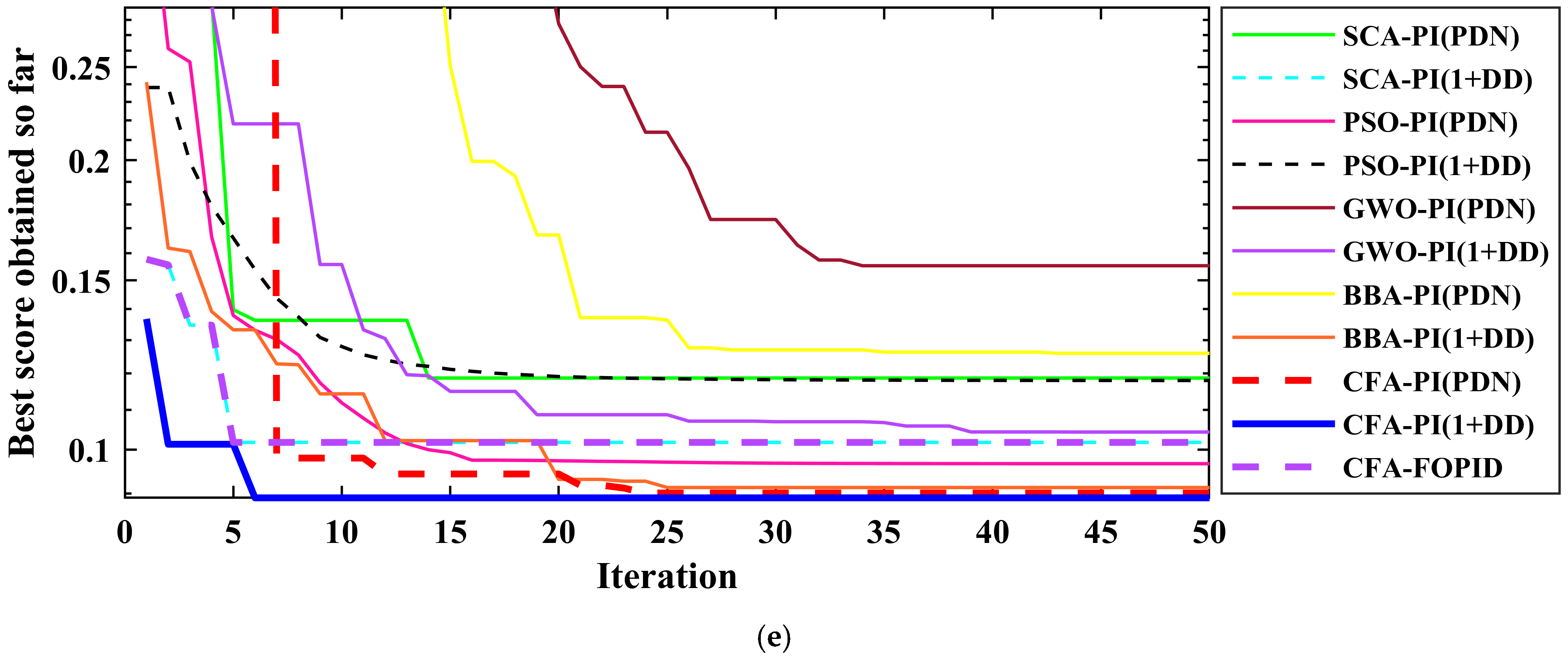Figure 11e shows the convergence performance of each optimization approach for tuning the controllers, with the highest score shown across iterations. The suggested CFA-PI-(1+DD) controller (in blue) quickly achieves a low score, indicating efficient convergence. This demonstrates the CFA’s success in attaining optimal tuning with fewer iterations, resulting in quicker and more consistent performance.

The figures show that the suggested CFA-PI-(1+DD) controller outperforms conventional control approaches for preserving frequency and tie-line power stability under random load disturbances. The CFA-PI-(1+DD) controller achieves faster convergence, lower frequency deviations, and reliable tie-line power exchange, making it ideal for load frequency management in linked renewable energy systems compared to others such as CFA-FOPID, CFA-PI-(PDN), CFA-PID, CFA-PI, and other controllers.

5.4. Case Four: Regular Renewable Energy Varying

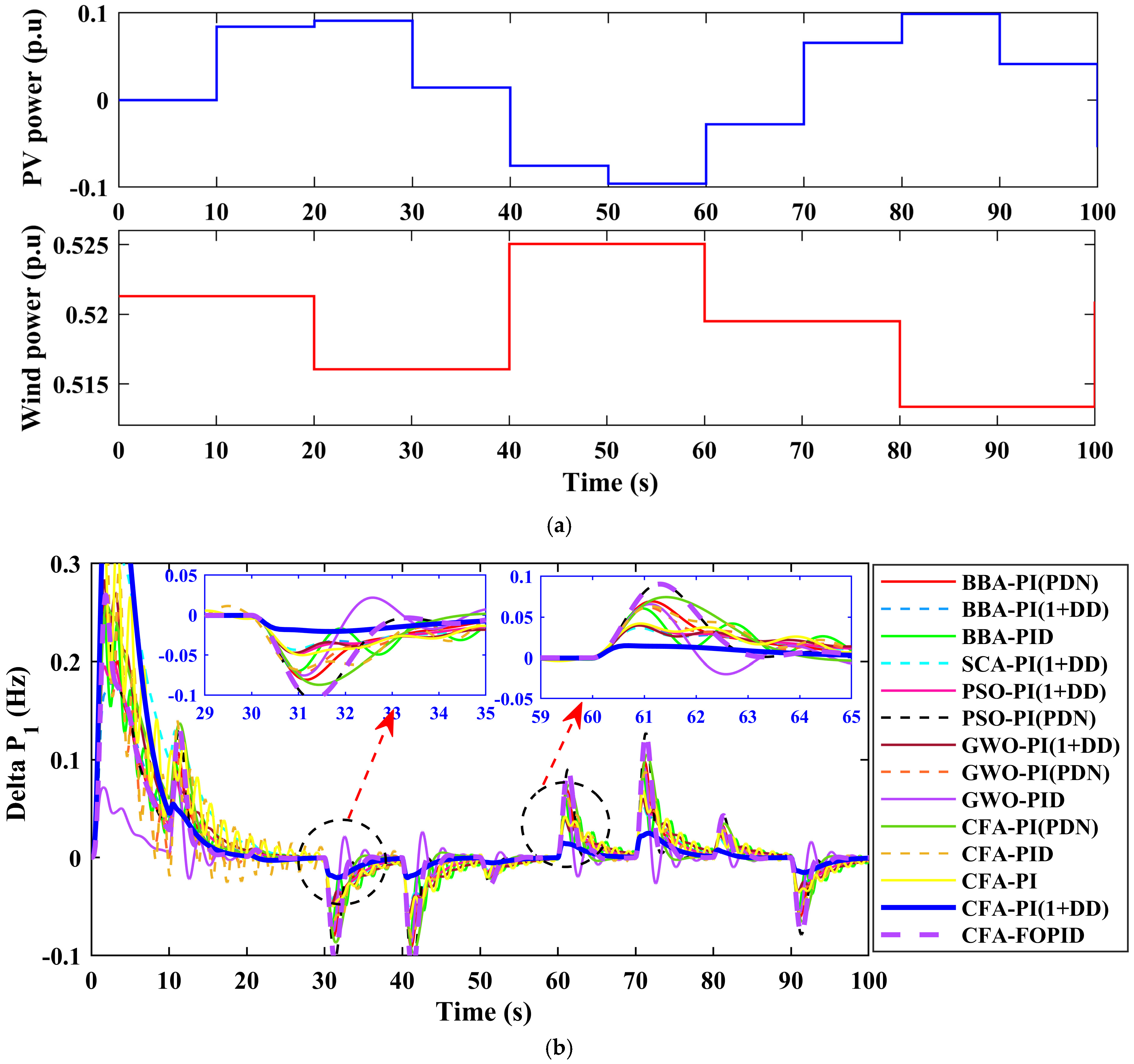
Figure 12a depicts the fluctuation in PV (blue line) and wind (red line) power throughout a 100 s simulation period. The step changes reflect the usual swings in renewable energy output. PV power ranges from −0.1 to 0.1 p.u., whereas wind power swings within a small range of 0.515–0.525 p.u. These changes imitate the typical renewable energy swings, which influence load frequency control.

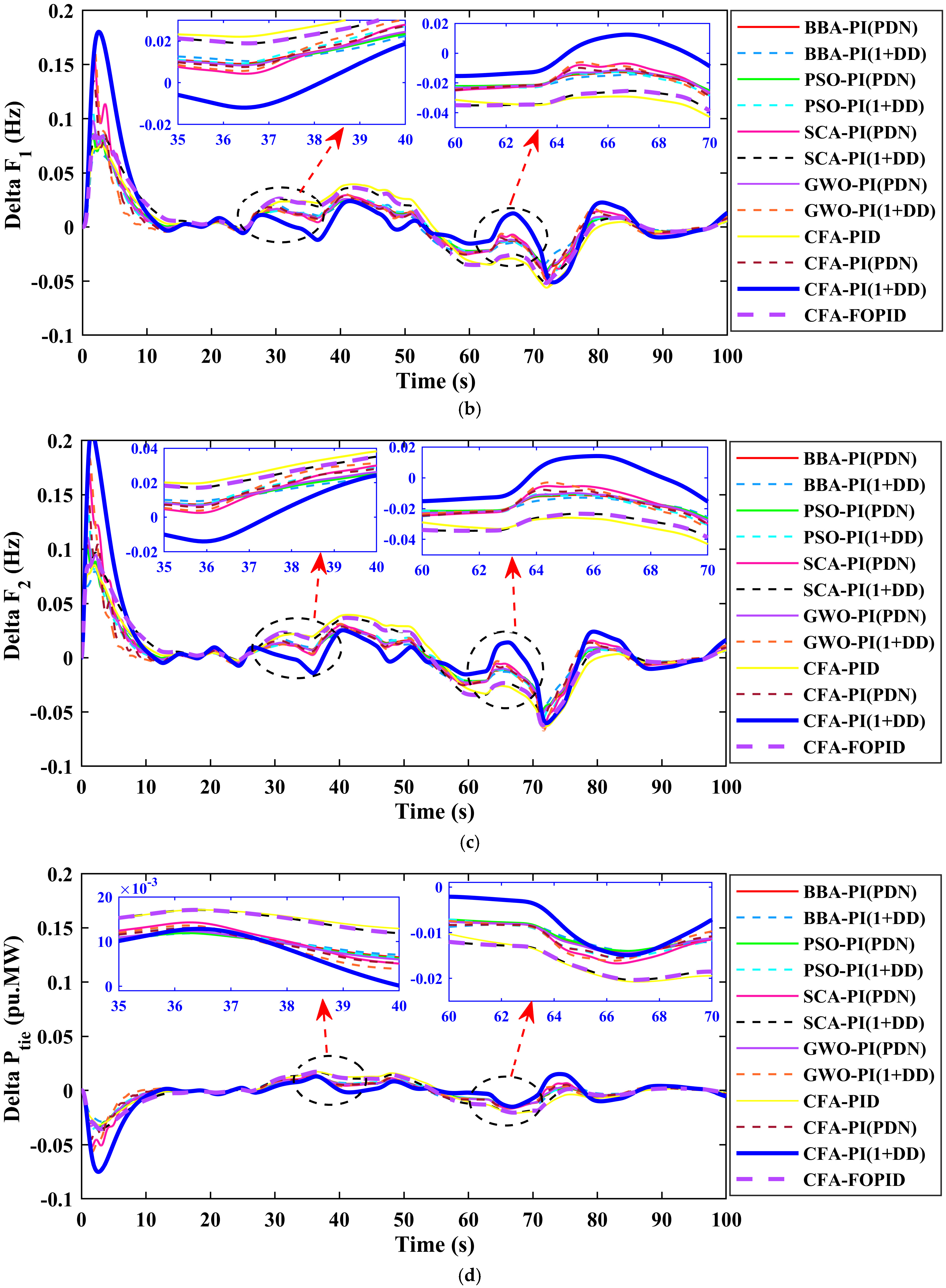
Figure 12b,c depict the frequency deviation in Areas 1 and 2 as a function of renewable power fluctuations (PV in Area 1 and wind in Area 2). Each line represents a distinct control technique that has been optimized using various optimization algorithms. The suggested CFA-PI-(1+DD) controller exhibits minimum frequency deviation and excellent oscillation damping, indicating a rapid reaction to renewable power changes. The zoomed-out graphic focuses on specific intervals, revealing transient reactions where the CFA-PI-(1+DD) controller outperforms other controllers such as CFA-FOPID, CFA-PI-(PDN), CFA-PID, CFA-PI, and other controllers in terms of frequency deviation stabilization.

Figure 12d shows the tie-line power variation (ΔPtie) between Areas 1 and 2, indicating power exchange stability with renewable power fluctuations. The CFA-PI-(1+DD) controller significantly reduces the tie-line power variations, resulting in synchronized power exchange. The insets focus on transient periods, where CFA-PI-(1+DD) achieves quick stabilization with minimum oscillations, surpassing other control schemes for managing power flow across related areas.

Figure 12e shows the convergence of each optimization approach for adjusting the controllers under renewable power changes. The best score acquired thus far is displayed across iterations, with the CFA-PI-(1+DD) controller (blue line) demonstrating rapid and consistent convergence. This demonstrates that the CFA effectively determines optimal tuning parameters, making it appropriate for dealing with the dynamic effects of renewable energy in load frequency management.

The outcomes of this analysis prove that the CFA-PI-(1+DD) controller excels at preserving frequency stability and minimizing tie-line power variances in the face of frequent renewable power variability. It provides rapid convergence, low frequency variations, and efficient power balancing, demonstrating its durability in systems with variable renewable energy sources compared to other controllers such as CFA-FOPID, CFA-PI-(PDN), CFA-PID, and CFA-PI.

5.5. Case Five: Stochastic PV Power Curves in Area 1 and WT Area 2

Figure 13a depicts the random fluctuations in PV (blue line) and wind (red line) power over a 100 s period, which simulates the unpredictable nature of renewable energy generation. The PV power gradually builds to a peak about 50 s before decreasing, whereas wind power fluctuates somewhat around a baseline value. This random variation examines the controller’s ability to adjust to variable renewable energy inputs. Figure 13b,c show the frequency deviation in Areas 1 and 2 after random renewable power variations. Each curve represents a separate controller tweaked by various optimization strategies. The CFA-PI-(1+DD) controller has low frequency deviations, indicating successful stabilization despite the variability in renewable power inputs. The insets show transient occurrences where the CFA-PI-(1+DD) controller performs better, with less fluctuations and quicker settling than other techniques such as CFA-FOPID, CFA-PI-(PDN), CFA-PID, and CFA-PI.

Figure 13d shows the tie-line power variation (ΔPtie) between Area 1 and Area 2 with random renewable power adjustments. The CFA-PI-(1+DD) controller successfully reduces tie-line deviations, ensuring that power is evenly distributed between the two zones. The insets emphasize specific intervals, demonstrating that the CFA-PI-(1+DD) controller maintains stability with low oscillations, outperforming conventional controllers in controlling tie-line power under random renewable variations. Figure 13e depicts the convergence of many optimization techniques for tuning controllers in the presence of unpredictable renewable energy changes. The best score attained thus far is displayed across iterations. The CFA-PI-(1+DD) controller quickly converges to a low error value, suggesting efficient and stable tuning. This demonstrates the CFA’s capacity to swiftly establish optimal tuning settings, despite the dynamic influence of random renewable fluctuations compared to CFA-FOPID, CFA-PI-(PDN), CFA-and PID, and CFA-PI controllers.

The output results mentioned above indicate that the CFA-PI-(1+DD) controller functions effectively in the presence of random renewable power changes, preserving frequency stability in both regions while minimizing tie-line power variances. It demonstrates rapid convergence and durable performance, highlighting its ability to handle unpredictable renewable energy swings in multi-area linked networks comparing to CFA-FOPID, CFA-PI-(PDN), CFA-PID, and CFA-PI controllers.

5.6. Sensitivity Analysis

In this section, the proposed CFA-tuned PI(1+DD) control strategy’s robustness was evaluated in a two-area IPS with an LFC system compared to other algorithms (PSO, BBO, SCA, GWO, and CFA, respectively) that are shown in Figure 14a–e. The speed regulation (R) and frequency bias coefficient (B) were simultaneously changed to  ± 25% of their nominal values. In this investigation, the proposed CFA-tuned PI(1+DD) controller’s optimal parameters are taken from Table 1. Figure 14 illustrates the load frequency, and tie-lie power responses of the proposed CFA-tuned PI(1+DD) control strategy with variations in R and B. Despite the ±25% variance in system parameters, it is clear from the results that the load frequency and tie-line power deviation responses are nearly identical to one another. The fact that values of all performance specifications including settling time, % overshoot, undershoot, and steady-state error have barely changed with variation in system parameters is proof that the proposed CFA-tuned PI(1+DD) can function well under dynamic circumstances.

Figure 14e presents a sensitivity analysis of the proposed CFA-tuned PI(1+DD) controller under ±25% variations in the system regulation parameters (R) and frequency bias coefficients (B). The results clearly demonstrate the robustness and adaptability of the controller. Frequency deviations in both Area 1 and Area 2 remain minimal and quickly return to nominal values across all tested parameter variations, indicating strong disturbance rejection and effective dynamic performance. Similarly, tie-line power deviations are well controlled, with smooth transitions and no overshoots or instability observed. The zoomed-in views further highlight the controller’s consistent response under parameter perturbations. Additionally, the convergence plot illustrates that the catch fish algorithm achieves rapid optimization, reaching the best score in very few iterations regardless of parameter changes. This confirms not only the computational efficiency of CFA but also the stability of its tuning process. Overall, the proposed method demonstrates superior performance and robustness compared to conventional techniques, maintaining system stability and control effectiveness even under significant parameter uncertainties. The results obtained categorically demonstrate that the recommended, proposed CFA-tuned PI(1+DD) controller is quite robust and does not require re-tuning for  ± 25% variations in R and B.

6. Conclusions

This research shows the LFC of a linked power system with two sectors integrated with renewable energy such as PV and wind. In the secondary loop, traditional PID and PI controllers are used to reduce frequency and tie-line power changes as quickly as feasible following several load disruptions. To begin, this study optimized the PID controller for each linked region by combining the CFA method with an IAE-based fitness function. According to the outcomes of the simulations carried out during five different cases, the CFA-tuned PID controller performs better than SCA-, BBA-, GWO-, and PSO-based optimization approaches in regards of peaking overshoot (+ve and −ve) values, of the frequency deviation of the power system, and the time (ts) it takes for variations to settle in a renewable energy-integrated power system. According to the literature, modifying the PID controller design results in greater efficiency than the typical PID control. According to the above declaration, this paper considers three cascaded types of PI(1+DD), FOPID, and PI(PDN) controllers to prove the effectiveness and robustness of the proposed CFA optimization approach. The simulation findings show that performance is improved with cascaded PI(1+DD), FOPID, and PI(PDN) controllers when compared to typical PID and PI controllers. The outcomes of this study provide verification to support the assumption that the CFA optimization strategy delivers superior controller performance than other existing optimization strategies such as SCA, GWO, PSO, and BBA. The following is a summary of this study’s primary findings:

• The RES-integrated two-area LFC system first considers typical PID, PI, PI(1+DD), FOPID, and PI(PDN) controllers. The settings of PID, PI, PI(1+DD), FOPID, and PI(PDN) controllers are adjusted using various optimization approaches, including CFA, SCA, BBA, GWO, and PSO.
• Apart from load instabilities in the area connected to the system, solar and wind turbine power variations are taken into account to confirm the control effectiveness in more accurate circumstances.
• The robustness and sensitivity of the CFA-, SCA-, BBA-, GWO-, and PSO-tuned controllers have been assessed in a variety of scenarios involving a range of step load disturbances and RES, including wind turbine and PV systems.
• This study found that the proposed CFA-tuned PI(1+DD) controller system outperformed the SCA-, BBA-, GWO-, and PSO-tuned PID controllers in terms of overshoot values and settling time in both areas.
• In addition, this work employs the suggested CFA optimization approach to adjust the FOPID and PI(PDN) controllers for the cascades under both constant and fluctuating load situations while integrating various renewable sources. The analysis’s findings demonstrated how well the CFA-tuned cascades PI(1+DD) controller performed in comparison to traditional PID, PI, FOPID, and PI(PDN) controllers.
• This study’s conclusions show that the cascade- PI(1+DD) controller’s performance is successfully improved by the CFA optimization approach. This improvement was shown when the system was fueled by renewable energy sources and operated under various load circumstances in addition to standard operating settings.

This performance study concludes that when compared to other optimization methods like SCA, BBA, GWO, and PSO, the CFA-tuned controllers show better control and reaction. The suggested CFA optimization method has no method-specific factors and is computationally effective. This implies that there is potential for improving controller performance in a variety of systems using the CFA optimization approach. For academics and practitioners looking for efficient optimization techniques for conventional and cascade controllers, this study’s conclusions offer insightful information. To examine the CFA optimization technique’s suitability for various control systems and assess its effectiveness across a larger variety of variables and circumstances, more investigation and analysis may be carried out.

Limitations of the Advanced PID-CFA Approach

(i)

While the integration of CFA with PID-based controllers has demonstrated strong performance in load frequency control for renewable-integrated power systems, there are inherent limitations to this approach. Firstly, PID controllers—despite their simplicity and widespread use—are inherently linear and thus may struggle to effectively control highly nonlinear systems or systems with large parameter uncertainties. In rapidly changing grid conditions or in the presence of highly intermittent renewable power sources, the controller may require frequent re-tuning to maintain optimal performance.

(ii)

Secondly, although CFA generally provides a faster convergence and global search ability, its performance can still be sensitive to the definition of objective functions and parameter bounds. In some complex or highly constrained systems, CFA may converge prematurely or require more computation time to reach an optimal solution compared to hybrid or adaptive algorithms.

(iii)

Moreover, PID-CFA designs may not be sufficient when precise tracking, robustness to high uncertainty, or adaptive real-time control are needed. In such cases, advanced model predictive control (MPC), robust control, or machine learning-based controllers could offer a better performance.

(iv)

Future work may focus on integrating CFA with adaptive or nonlinear control strategies and investigating its real-time implementation feasibility under uncertain and rapidly varying grid environments.

(v)

While the simulation results clearly demonstrate the effectiveness of the proposed CFA-optimized advanced PID controllers for LFC, namely PI, PID, fractional-order PID (FOPID), PI with derivative and delay [PI(1+DD)], and cascaded PI [PI(PDN)] for enhancing the dynamic frequency response of a two-area interconnected non-reheat thermal power system integrated with renewable energy sources such as PV and wind power. We acknowledge that real-world validation is essential to fully assess the practical applicability of this method. Future work will focus on experimental implementation using a real-time simulation platform such as OPAL-RT or MATLAB Simulink Real-Time to emulate the actual system conditions. This will allow for validation against physical data and real disturbances, thereby enhancing the reliability and applicability of the proposed approach in real power-system environments.