Dynamical Analysis of Mpox Disease with Environmental Effects

Abstract

In this study, we develop a fractional-order mathematical model for investigating the transmission dynamics of monkeypox (Mpox), accounting for interactions between humans, rodents, and environmental reservoirs. The model uniquely integrates two key control strategies—public health awareness and environmental sanitation—often overlooked in previous models. We analyze the model’s well-posedness by establishing the existence, uniqueness, and positivity of solutions using the fixed-point theorem. Using data from the Democratic Republic of Congo, we estimate the model parameters and demonstrate that the fractional-order model ($\varphi =0.5$) fits real-world data more accurately than its integer-order counterpart ($\varphi =1$). The sensitivity analysis using partial rank correlation coefficients highlights the key drivers of disease spread. Numerical simulations reveal that the memory effects inherent in fractional derivatives significantly influence the epidemic’s trajectory. Importantly, our results show that increasing awareness ($ϵ$) and sanitation efforts ($\eta$) can substantially reduce transmission, with sustained suppression of Mpox when both parameters exceed $90\%$. These findings highlight the synergistic impact of behavioral and environmental interventions in controlling emerging zoonotic diseases.

1. Introduction

Monkeypox is a rare but potentially serious zoonotic disease caused by the monkeypox virus (MPXV) which belongs to the genus Orthopoxvirus within the family Poxviridae [1]. Common members of the Orthopoxvirus genus include the variola, vaccinia, cowpox, and monkeypox viruses [2]. Smallpox, a highly dangerous Orthopoxvirus, is believed to have caused over 300 million deaths worldwide before being eradicated in 1977 through a global vaccination campaign led by the World Health Organization (WHO) [3]. In 2022, the WHO reported multiple monkeypox outbreaks across 20 non-endemic European countries, as well as cases in the United States, Canada, Mexico, and several countries in South America [4]. In Africa, monkeypox remains endemic in parts of Central and West Africa, particularly in regions where humans frequently interact with wildlife [5]. The most affected African countries include Benin, Cameroon, the Central African Republic, the Democratic Republic of the Congo, Gabon, Ivory Coast, Liberia, Nigeria, Sierra Leone, and South Sudan [6]. Orthopoxvirus can be transmitted to humans through direct contact with infected animals such as rodents and primates or via human-to-human transmission through close contact with lesions, bodily fluids, or respiratory droplets [7], see Figure 1. The incubation period for monkeypox ranges from 7 to 17 days. Common clinical symptoms include fever, headache, swollen lymph nodes, muscle aches, chills, and skin lesions [8]. The transmission cycle of MPXV is presented in Figure 1.

Mathematical models are powerful tools for understanding the factors that influence the persistence or elimination of diseases, especially when field experiments are not feasible [10]. According to McKenzie [11], these models can help answer complex questions that may be difficult, costly, dangerous, or impractical to investigate through other methods. Recently, epidemiological models for smallpox have been developed to explore various factors, such as the effects of quarantine and isolation [12], prevention measures, treatment of infected individuals [13], vaccination and awareness [14], and environmental contamination [15]. For mathematical models of monkeypox transmission that include control strategies, readers may refer to [16,17,18,19,20,21,22,23,24] and the references therein. Despite these efforts, several challenges remain in the mathematical modeling of monkeypox. One major limitation is the knowledge gap regarding the combined effects of environmental sanitation and human awareness on disease transmission. The majority of the existing monkeypox transmission models have primarily focused on the effects of vaccination (see [25,26,27,28,29,30,31,32] and the references therein). However, it is well known that its rising prevalence in humans has been linked to waning immunity, posing a growing public health threat [33].

Health education campaigns play a vital role in raising awareness about the transmission, symptoms, and prevention of monkeypox [34]. Many rural communities, particularly in Africa, lack adequate knowledge about this disease, leading to delayed reporting and increased spread [35]. Such campaigns can also help correct misinformation and encourage early detection and treatment [27]. Regarding environmental sanitation, improving hygiene can reduce monkeypox’s transmission by limiting human contact with contaminated surfaces and infected animals [36]. In contrast, poor sanitation attracts rodents, which are known reservoirs of the virus [37].

Recently, mathematical models incorporating fractional-order differential equations have gained significant attention (see [3,38,39,40,41,42]) and have been shown to provide more accurate results in disease modeling than integer-order derivatives [43]. Fractional-order operators introduce additional degrees of freedom [34], enabling greater precision in modeling. Notably, these operators have several advantages over the classical integer-order models, as they effectively capture the memory effects, long-range interactions, and hereditary properties found in biological systems [44,45]. In contrast, models based on integer-order derivatives fail to fully represent these characteristics [10]. Moreover, fractional-order models demonstrate higher precision and a better fit to real-world data [39]. While we have conducted our own literature review to identify existing mathematical models for Mpox transmission, we also refer the reader to the comprehensive scoping review by Molla et al. [46] for an in-depth survey of the recent modeling approaches.

Motivated by the above discussion, this study aims to investigate the combined effects of human awareness and environmental sanitation on monkeypox transmission dynamics. To the best of our knowledge, no fractional-order model of monkeypox’s transmission has been formulated to incorporate both of these control strategies. Therefore, we propose a novel fractional-order model that integrates two key interventions—health education awareness and environmental sanitation—and assess their effectiveness in minimizing the spread of monkeypox within the population.

The rest of this paper is organized as follows: In Section 2, the mathematical model’s formulation is presented. Section 3 addresses the existence and uniqueness of the solutions, the positivity of the variables, and the boundedness of the trajectories. Section 4 provides the computation of the basic reproduction number and analyzes the existence of model equilibria. The results and discussion are presented in Section 5. Finally, concluding remarks are given in Section 6.

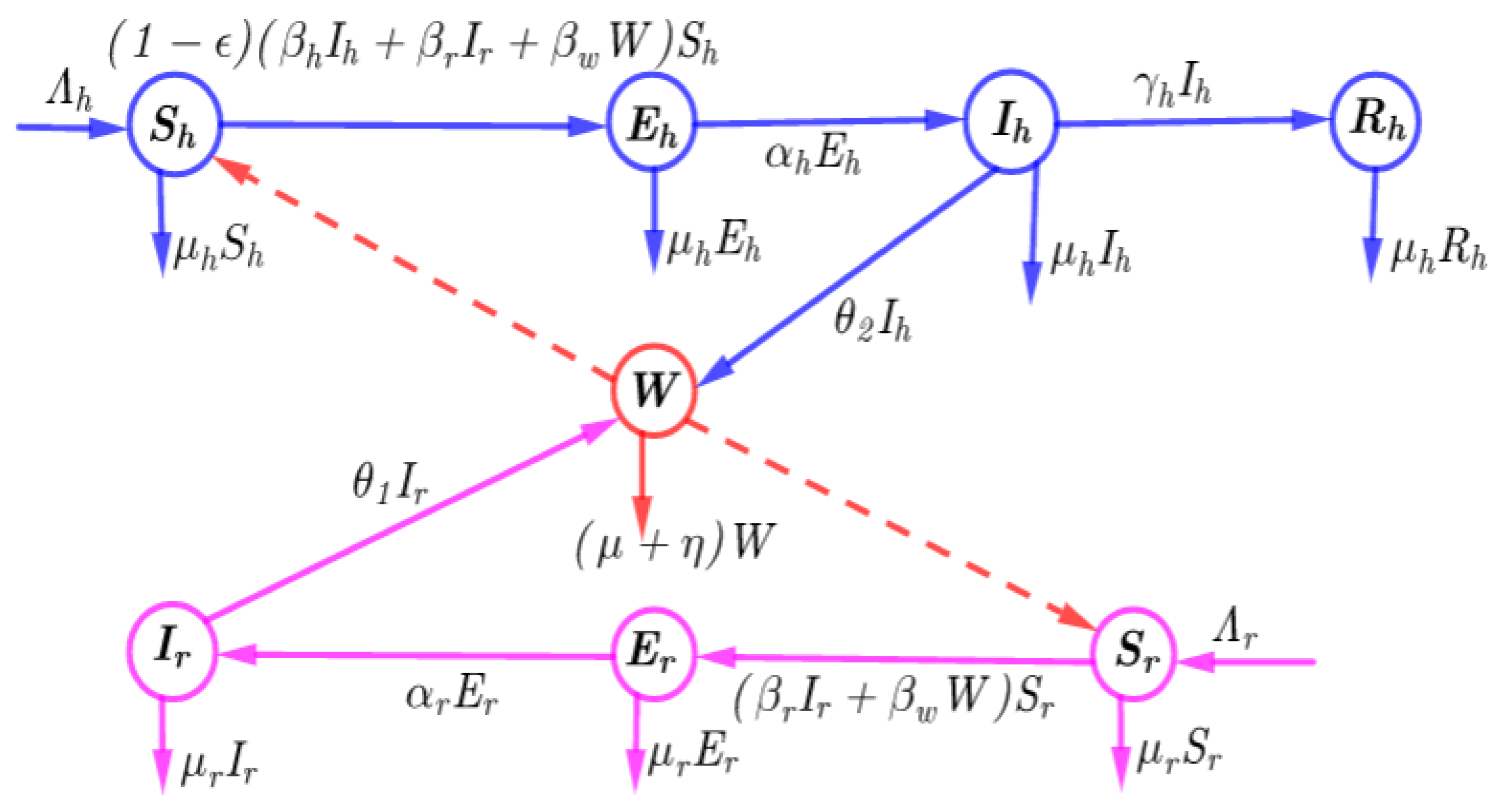
2. Model Formulation

In this research work, we propose and formulate a mathematical model of Mpox disease transmission that includes the interplay between human, animal (rodent), and environmental effects. Throughout this document, the subscripts h and r, respectively, denote the human and rodent populations. The main assumption in the proposed model is that both the humans and the rodents shed the virus into the environment. Naive susceptible humans acquire infections from either an infected human or rodent or from the contaminated environment. On the other hand, susceptible rodents acquire an infection from either infected rodents or the contaminated environment. The human population is sub-divided into four groups based on infection status, namely susceptible $S_h\left(t\right)$, exposed $E_h\left(t\right)$, infectious $I_h\left(t\right)$, and recovered $R_h\left(t\right)$ classes. Thus, the total population of humans at time t is denoted by $N_h\left(t\right)$ and given as

$$\begin{array}{c}\hfill N_h\left(t\right)=S_h\left(t\right)+E_h\left(t\right)+I_h\left(t\right)+R_h\left(t\right)\end{array}$$

(1)

Furthermore, the total population of rodents at time t is denoted by $N_r\left(t\right)$ and is sub-divided into three groups, namely susceptible $S_r\left(t\right)$, exposed $E_r\left(t\right)$, and infectious $I_r\left(t\right)$ classes. Thus, the total population of rodents at time t is defined by

$$\begin{array}{c}\hfill N_r\left(t\right)=S_r\left(t\right)+E_r\left(t\right)+I_r\left(t\right)\end{array}$$

(2)

The contamination of the environment by the virus at time t is denoted by $M\left(t\right)$. All of the parameters and variables of the proposed model are assumed to be positive, and the parameters are described as follows: ${\mathrm{\Lambda }}_h$ and ${\mathrm{\Lambda }}_r$ denote the new recruitment rates of humans and rodents, respectively, and all are considered to be susceptible whether originating from either being newly born into the environment or immigrating; ${\mu }_h$ and ${\mu }_r$ denote the natural mortality rates of humans and rodents, respectively; ${\alpha }_h$ and ${\alpha }_r$ denote the transfer rates of humans and rodents, respectively, from the exposed class to the infectious class; ${\gamma }_h$ represents the recovery rate of infected humans; and $d_h$ denotes the disease-induced death rate of infected humans. We have assumed that susceptible individuals acquire an infection following effective contact with either the contaminated environment or humans or rodents displaying clinical symptoms of the disease. Thus, we consider the following forces of infection for humans and rodents, respectively: ${\beta }_h$ and ${\beta }_r$. The parameters ${\beta }_m$ and ${\beta }_r$ denote the forces of infection due to environmental contamination and infected rodents, respectively, while K denotes the half-saturation constant of the virus in environment. Furthermore, we assume that infected humans and rodents shed the virus into the environment at the rates ${\theta }_2$ and ${\theta }_1$, respectively. The parameter $\mu$ denotes the natural decay of the virus in the environment, and $\eta$ represents the rate of decay of the virus in the environment due to cleanness. In addition, we have assumed the parameter $ϵ$ to capture the effects of health education campaigns, while $\sigma$ denotes the effects of environmental cleanness. Based on the above assumptions, we have assumed the following flowchart and non-linear differential equations:

From the flowchart diagram in Figure 2, the dynamics of the interaction between humans and rodents in the contaminated environment is given by the following system of ordinary differential equations:

$$\left\{\begin{array}{ccc}{\displaystyle {}_{t_0}{}^{c}D_t^{\varphi }{S}_h\left(t\right)}\hfill & =\hfill & {\displaystyle {\mathrm{\Lambda }}_h-(1-ϵ)\left({\beta }_h{I}_h\left(t\right)+{\beta }_r{I}_r\left(t\right)+{\beta }_{w}W\left(t\right)\right)S_h\left(t\right)-{\mu }_h{S}_h\left(t\right),}\hfill \\ {\displaystyle {}_{t_0}{}^{c}D_t^{\varphi }{E}_h\left(t\right)}\hfill & =\hfill & {\displaystyle (1-ϵ)\left({\beta }_h{I}_h\left(t\right)+{\beta }_r{I}_r\left(t\right)+{\beta }_{w}W\left(t\right)\right)S_h\left(t\right)-({\mu }_h+{\alpha }_h)E_h\left(t\right),}\hfill \\ {\displaystyle {}_{t_0}{}^{c}D_t^{\varphi }{I}_h\left(t\right)}\hfill & =\hfill & {\displaystyle {\alpha }_h{E}_h\left(t\right)-({\mu }_h+d_h+{\gamma }_h)I_h\left(t\right),}\hfill \\ {\displaystyle {}_{t_0}{}^{c}D_t^{\varphi }{R}_h\left(t\right)}\hfill & =\hfill & {\displaystyle {\gamma }_h{I}_h\left(t\right)-{\mu }_h{R}_h\left(t\right),}\hfill \\ {\displaystyle {}_{t_0}{}^{c}D_t^{\varphi }W\left(t\right)}\hfill & =\hfill & {\displaystyle {\theta }_1{I}_r\left(t\right)+{\theta }_2{I}_h-(\mu +\eta )W\left(t\right),}\hfill \\ {\displaystyle {}_{t_0}{}^{c}D_t^{\varphi }{S}_r\left(t\right)}\hfill & =\hfill & {\displaystyle {\mathrm{\Lambda }}_r-\left({\beta }_r{I}_r\left(t\right)+{\beta }_{w}W\left(t\right)\right)S_r\left(t\right)-{\mu }_r{S}_r\left(t\right),}\hfill \\ {\displaystyle {}_{t_0}{}^{c}D_t^{\varphi }{E}_r\left(t\right)}\hfill & =\hfill & {\displaystyle \left({\beta }_r{I}_r\left(t\right)+{\beta }_{w}W\left(t\right)\right)S_r\left(t\right)-({\mu }_r+{\alpha }_r)E\left(t\right),}\hfill \\ {\displaystyle {}_{t_0}{}^{c}D_t^{\varphi }{I}_r\left(t\right)}\hfill & =\hfill & {\displaystyle {\alpha }_r{E}_r\left(t\right)-{\mu }_r{I}_r\left(t\right).}\hfill \end{array}\right.$$

(3)

3. Model Analysis

3.1. Preliminaries on the Caputo Fractional Calculus

We begin by introducing the concept and relevant theorems of Caputo fractional differential equations ([44,47,48,49]). The theorem and concepts defined herein are useful for the proposed study.

Definition 1.

If we consider that $\varphi >0,t>a,\varphi a,t\in \mathbb{R},$ then we can define the Caputo fractional derivative as follows:

$$\begin{array}{c}\hfill {}_0{}^{c}D_t^{\varphi }f\left(t\right){\displaystyle \frac{1}{\mathrm{\Gamma }(n-\varphi )}}{\int }_a^t{\displaystyle \frac{f^n\left(\xi \right)}{{(t-\xi )}^{\varphi +1-n}}}d\xi ,n-1<\varphi ,n\in \mathbb{N}.\end{array}$$

(4)

Definition 2.

The Caputo fractional derivative for a constant function $f\left(t\right)=c$ (see [44]) is defined as follows:

$$\begin{array}{c}\hfill {}_0{}^{c}D_t^{\varphi }c=0,\varphi \in (0,1)\end{array}$$

(5)

Definition 3.

The fractional calculus in Liouville–Caputo derivatives is given as follows:

$$\begin{array}{c}\hfill {}_0{}^{c}D_t^{\varphi }f\left(t\right)={\displaystyle \frac{N\left(\varphi \right)}{1-\varphi }}{\int }_0^t{f}^{\prime }\left(\tau \right)exp\left[{\displaystyle \frac{\varphi (t-\tau )}{1-\tau }}\right]d\tau \end{array}$$

(6)

whereby $N\left(\varphi \right)$ is defined as $N\left(0\right)=N\left(1\right)=1$.

Definition 4.

The integral calculus in the Caputo sense of the function $f\left(t\right)$ is defined as follows:

$$\begin{array}{c}\hfill {}_0{}^{c}I_t^{\varphi }f\left(t\right)={\displaystyle \frac{2(1-\varphi )}{(2-\varphi )N\left(\varphi \right)}}f\left(t\right)+{\displaystyle \frac{2\varphi }{(2-\varphi )N\left(\varphi \right)}}{\int }_0^{t}f\left(s\right)ds,t\ge 0\end{array}$$

(7)

whereby $N\left(\varphi \right)={\displaystyle \frac{2}{2-\varphi }},0<\varphi \le 1$.

3.2. The Existence and Uniqueness of the Solution

In this part, we present the existence and uniqueness of the solution of the model system (3). Let us define the Banach space equipped with the norm by $\mathcal{B}=\ell \left(\right[0,T],\Re )$, which is given as

$$\begin{array}{c}\left|\right|S_h,E_h,I_h,R_h,W,S_r,E_r,I_r\left|\right|=\left|\right|S_h\left|\right|+\left|\right|E_h\left|\right|+\left|\right|I_h\left|\right|+\left|\right|R_h|+|\left|W\right||+||S_r\left|\right|+\left|\right|E_r\left|\right|+\left|\right|I_r\left|\right|,\hfill \end{array}$$

where

$$\begin{array}{c}||S_h\left(t\right)||=\underset{t\in [0,T]}{sup}|S_h\left(t\right)|,||E_h\left(t\right)||=\underset{t\in [0,T]}{sup}|E_h\left(t\right)|,||I_h\left(t\right)||=\underset{t\in [0,T]}{sup}|I_h\left(t\right)|,||R_h\left(t\right)||=\hfill \\ \underset{t\in [0,T]}{sup}|R_h\left(t\right)|,|W\left(t\right)||=\underset{t\in [0,T]}{sup}|W\left(t\right)|,||S_r\left(t\right)||=\underset{t\in [0,T]}{sup}|S_r\left(t\right)|,\hfill \\ ||E_r\left(t\right)||=\underset{t\in [0,T]}{sup}|E_r\left(t\right)|,||I_r\left(t\right)||=\underset{t\in [0,T]}{sup}|I_r\left(t\right)|.\hfill \end{array}$$

Next, we consider the following fractional integral operator ${}^{c}I_{0+}^{\varphi }$ on both sides of the system (3):

$$\left.\begin{array}{ccc}{\displaystyle S_h\left(t\right)-S_h\left(0\right)}\hfill & =\hfill & {\displaystyle {}^{c}I_{0+}^{\theta }\left\{{\mathrm{\Lambda }}_h-(1-ϵ)\left({\beta }_h{I}_h\left(t\right)+{\beta }_r{I}_r\left(t\right)+{\beta }_{w}W\left(t\right)\right)S_h\left(t\right)-{\mu }_h{S}_h\left(t\right)\right\},}\hfill \\ {\displaystyle E_h\left(t\right)-E_h\left(0\right)}\hfill & =\hfill & {\displaystyle {}^{c}I_{0+}^{\theta }\{(1-ϵ)\left({\beta }_h{I}_h\left(t\right)+{\beta }_r{I}_r\left(t\right)+{\beta }_{w}W\left(t\right)\right)S_h\left(t\right)}\hfill \\ \hfill & \hfill & -({\mu }_h+{\alpha }_h)E_h\left(t\right)\},\hfill \\ {\displaystyle I_h\left(t\right)-I_h\left(0\right)}\hfill & =\hfill & {\displaystyle {}^{c}I_{0+}^{\theta }\left\{{\alpha }_h{E}_h\left(t\right)-({\mu }_h+d_h+{\gamma }_h)I_h\left(t\right)\right\},}\hfill \\ {\displaystyle R_h\left(t\right)-R_h\left(0\right)}\hfill & =\hfill & {\displaystyle {}^{c}I_{0+}^{\theta }\left\{{\gamma }_h{I}_h\left(t\right)-{\mu }_h{R}_h\left(t\right)\right\},}\hfill \\ {\displaystyle M\left(t\right)-M\left(0\right)}\hfill & =\hfill & {\displaystyle {}^{c}I_{0+}^{\theta }\left\{{\theta }_1{I}_r\left(t\right)+{\theta }_2{I}_h-(\mu +\eta )M\left(t\right)\right\},}\hfill \\ {\displaystyle S_r\left(t\right)-S_r\left(0\right)}\hfill & =\hfill & {\displaystyle {}^{c}I_{0+}^{\theta }\left\{{\mathrm{\Lambda }}_r-\left({\beta }_r{I}_r\left(t\right)+{\beta }_{w}W\left(t\right)\right)S_r\left(t\right)-{\mu }_r{S}_r\left(t\right)\right\},}\hfill \\ {\displaystyle E_r\left(t\right)-E_r\left(0\right)}\hfill & =\hfill & {\displaystyle {}^{c}I_{0+}^{\theta }\left\{\left({\beta }_r{I}_r\left(t\right)+{\beta }_{w}W\left(t\right)\right)S_r\left(t\right)-({\mu }_r+{\alpha }_r)E\left(t\right)\right\},}\hfill \\ {\displaystyle I_v\left(t\right)-I_v\left(0\right)}\hfill & =\hfill & {\displaystyle {}^{C}I_{0+}^{\theta }\left\{{\alpha }_r{E}_r\left(t\right)-{\mu }_r{I}_r\left(t\right)\right\}.}\hfill \end{array}\right\}$$

(8)

This shows that for $k=1,2,3\dots 8$, one obtains the following:

$${\displaystyle \begin{array}{ccc}{S}_h\left(t\right)\hfill & =\hfill & {\displaystyle S_h\left(0\right)+\frac{(1-\varphi )}{N\left(\varphi \right)}(F_i(t,S_h\left(t\right))+\frac{\varphi }{N\left(\theta \right)}\frac{1}{\mathrm{\Gamma }\left(\varphi \right)}{\int }_0^t{F}_k(t,S_h\left(t\right))d\tau ,}\hfill \\ E_h\left(t\right)\hfill & =\hfill & {\displaystyle E_h\left(0\right)+\frac{(1-\varphi )}{N\left(\varphi \right)}(F_k(t,E_h\left(t\right))+\frac{\varphi }{N\left(\varphi \right)}\frac{1}{\mathrm{\Gamma }\left(\varphi \right)}{\int }_0^t{F}_k(t,E_h\left(t\right))d\tau ,}\hfill \\ I_h\left(t\right)\hfill & =\hfill & I_h\left(0\right)+\frac{(1-\varphi )}{N\left(\varphi \right)}(F_k(t,I_h\left(t\right))+\frac{\varphi }{N\left(\varphi \right)}\frac{1}{\mathrm{\Gamma }\left(\varphi \right)}{\int }_0^t{F}_k(t,I_h\left(t\right))d\tau ,\hfill \\ R_h\left(t\right)\hfill & =\hfill & R_h\left(0\right)+\frac{(1-\varphi )}{N\left(\varphi \right)}(F_k(t,R_h\left(t\right))+\frac{\varphi }{N\left(\varphi \right)}\frac{1}{\mathrm{\Gamma }\left(\varphi \right)}{\int }_0^t{F}_k(t,R_h\left(t\right))d\tau ,\hfill \\ M\left(t\right)\hfill & =\hfill & M\left(0\right)+\frac{(1-\varphi )}{N\left(\theta \right)}(F_k(t,N\left(t\right))+\frac{\varphi }{N\left(\varphi \right)}\frac{1}{\mathrm{\Gamma }\left(\varphi \right)}{\int }_0^t{F}_k(t,M\left(t\right))d\tau ,\hfill \\ S_r\left(t\right)\hfill & =\hfill & S_r\left(0\right)+\frac{(1-\varphi )}{N\left(\varphi \right)}(F_k(t,S_r\left(t\right))+\frac{\theta }{N\left(\varphi \right)}\frac{1}{\mathrm{\Gamma }\left(\varphi \right)}{\int }_0^t{F}_k(t,S_r\left(t\right))d\tau ,\hfill \\ E_r\left(t\right)\hfill & =\hfill & E_r\left(0\right)+\frac{(1-\varphi )}{N\left(\varphi \right)}(F_k(t,E_r\left(t\right))+\frac{\varphi }{N\left(\varphi \right)}\frac{1}{\mathrm{\Gamma }\left(\varphi \right)}{\int }_0^t{F}_k(t,E_r\left(t\right))d\tau ,\hfill \\ I_r\left(t\right)\hfill & =\hfill & I_r\left(0\right)+\frac{(1-\varphi )}{N\left(\varphi \right)}(F_k(t,I_r\left(t\right))+\frac{\varphi }{N\left(\varphi \right)}\frac{1}{\mathrm{\Gamma }\left(\varphi \right)}{\int }_0^t{F}_k(t,I_r\left(t\right))d\tau .\hfill \end{array}\}}$$

(9)

where

$$\left.\begin{array}{ccc}{F}_k(t,S_h\left(t\right))\hfill & =\hfill & {\mathrm{\Lambda }}_h-(1-ϵ)\left({\beta }_h{I}_h+{\beta }_r{I}_r+{\beta }_{w}W\right)S_h-{\mu }_h{S}_h,\hfill \\ F_k(t,E_h\left(t\right))\hfill & =\hfill & (1-ϵ)\left({\beta }_h{I}_h+{\beta }_r{I}_r+{\beta }_{w}W\right)S_h\hfill \\ \hfill & \hfill & -({\mu }_h+{\alpha }_h)E_h,\hfill \\ F_k(t,I_h\left(t\right))\hfill & =\hfill & {\alpha }_h{E}_h-({\mu }_h+d_h+{\gamma }_h)I_h,\hfill \\ F_k(t,R_h\left(t\right))\hfill & =\hfill & {\displaystyle {\gamma }_h{I}_h-{\mu }_h{R}_h,}\hfill \\ F_k(t,W\left(t\right))\hfill & =\hfill & {\displaystyle {\theta }_1{I}_r+{\theta }_2{I}_h-(\mu +\eta )W,}\hfill \\ F_k(t,S_r\left(t\right))\hfill & =\hfill & {\displaystyle \left({\beta }_r{I}_r+{\beta }_{w}W\right)S_r\left(t\right)-{\mu }_r{S}_r,}\hfill \\ F_k(t,E_r\left(t\right))\hfill & =\hfill & {\displaystyle \left({\beta }_r{I}_r+{\beta }_{w}W\right)S_r-({\mu }_r+{\alpha }_r)E,}\hfill \\ F_k(t,I_r\left(t\right))\hfill & =\hfill & {\displaystyle {\alpha }_r{E}_r-{\mu }_r{I}_r.}\hfill \end{array}\right\}$$

(10)

The given kernel N ($0\le Q_k<1,$) in (10) concurs with the Lipschitz condition if and only if $S_h,E_h,I_h,R_h,W,S_r,E_r,$ and $I_r$ have an upper bound. This implies that $S_h$ and $S_h^{*}$ are two functions and thus

$$\left.\begin{array}{ccc}\left|\right|F_{k}t,I_h\left(t\right)-F_k(t,I_h^{*}\left(t\right))\left|\right|\hfill & =\hfill & \left|\right|{\alpha }_h{E}_h-({\mu }_h+d_h+{\gamma }_h)I_h\hfill \\ \hfill & \hfill & -\left({\alpha }_h{E}_h-({\mu }_h+d_h+{\gamma }_h)I_h^{*}\right)\left|\right|,\hfill \\ \hfill & \hfill & =\left({\alpha }_h{E}_h\left(t\right)-({\mu }_h+d_h+{\gamma }_h)\right)\left|\right|I_h-I_h^{*}\left|\right|,\hfill \\ \hfill & \hfill & \le \left({\alpha }_h\underset{t\in [0,T]}{sup}{E}_h\left(t\right)+{\mu }_h+d_h+{\gamma }_h\right)\left|\right|I_h-I_h^{*}\left|\right|,\hfill \\ \hfill & \hfill & =Q_k\left|\right|I_h-I_h^{*}\left|\right|.\hfill \end{array}\right\}$$

(11)

where $Q_k={\alpha }_h{sup}_{t\in [0,T]}{E}_h\left(t\right)+{\mu }_h+d_h+{\gamma }_h$. Thus,

$$\begin{array}{c}\left|\right|F_{k}t,I_h\left(t\right)-F_k(t,I_h^{*}\left(t\right))\left|\right|\le Q_k\left|\right|I_h-I_h^{*}\left|\right|\hfill \end{array}$$

(12)

From (11), one can note that

$$\left.\begin{array}{ccc}\left|\right|F_{k}t,S_h-F_k(t,S_h^{*})\left|\right|\hfill & \le \hfill & Q_k\left|\right|S_h-S_h^{*}\left|\right|,\hfill \\ \left|\right|F_{k}t,E_h\left(t\right)-F_k(t,E_h^{*})\left|\right|\hfill & \le \hfill & Q_k\left|\right|E_h-E_h^{*}\left|\right|,\hfill \\ \left|\right|F_{k}t,R_h-F_k(t,R_h^{*})\left|\right|\hfill & \le \hfill & Q_k\left|\right|R_h-R_h^{*}\left|\right|,\hfill \\ \left|\right|F_{k}t,W_h\left(t\right)-F_k(t,W_h^{*})\left|\right|\hfill & \le \hfill & Q_k\left|\right|W_h-W_h^{*}\left|\right|,\hfill \\ \left|\right|F_{k}t,S_r-F_k(t,S_r^{*}\left(t\right))\left|\right|\hfill & \le \hfill & Q_k\left|\right|S_r-S_r^{*}\left|\right|,\hfill \\ \left|\right|F_{k}t,E_r-F_k(t,E_r^{*})\left|\right|\hfill & \le \hfill & Q_k\left|\right|E_r-E_r^{*}\left|\right|,\hfill \\ \left|\right|F_{k}t,I_r-F_k(t,I_r^{*}\left(t\right))\left|\right|\hfill & \le \hfill & Q_k\left|\right|I_r-I_r^{*}\left|\right|.\hfill \end{array}\right\}$$

(13)

whereby $Q_k$ is the Lipschitz constant for the function $F_k(.)$ Indeed, Equation (9) in recursive form is as follows:

$$\left.\begin{array}{ccc}{\displaystyle S_h}\hfill & =\hfill & {\displaystyle S_h\left(0\right)+\frac{(1-\varphi )}{N\left(\varphi \right)}{F}_k(t,S_{h,n-1}\left(t\right))+\frac{\varphi }{N\left(\varphi \right)}\frac{1}{\mathrm{\Gamma }\left(\varphi \right)}{\int }_0^t{(t-\sigma )}^{\varphi -1}{F}_k(\sigma ,S_{h,n-1}\left(\sigma \right))d\sigma ,}\hfill \\ {\displaystyle E_h}\hfill & =\hfill & {\displaystyle E_h\left(0\right)+\frac{(1-\varphi )}{N\left(\varphi \right)}{F}_k(t,E_{h,n-1}\left(t\right))+\frac{\varphi }{N\left(\varphi \right)}\frac{1}{\mathrm{\Gamma }\left(\varphi \right)}{\int }_0^t{(t-\sigma )}^{\varphi -1}{F}_k(\sigma ,E_{h,n-1}\left(\tau \right))d\sigma ,}\hfill \\ {\displaystyle I_h}\hfill & =\hfill & {\displaystyle I_h\left(0\right)+\frac{(1-\varphi )}{N\left(\varphi \right)}{F}_k(t,I_{h,n-1})+\frac{\varphi }{N\left(\varphi \right)}\frac{1}{\mathrm{\Gamma }\left(\varphi \right)}{\int }_0^t{(t-\sigma )}^{\varphi -1}{F}_k(\sigma ,E_{h,n-1}\left(\sigma \right))d\sigma ,}\hfill \\ {\displaystyle R_h}\hfill & =\hfill & {\displaystyle R_h\left(0\right)+\frac{(1-\varphi )}{N\left(\varphi \right)}{F}_k(t,R_{h,n-1}\left(t\right))+\frac{\varphi }{N\left(\varphi \right)}\frac{1}{\mathrm{\Gamma }\left(\varphi \right)}{\int }_0^t{(t-\sigma )}^{\varphi -1}{F}_k(\sigma ,R_{h,n-1}\left(\sigma \right))d\sigma ,}\hfill \\ {\displaystyle W}\hfill & =\hfill & {\displaystyle W\left(0\right)+\frac{(1-\varphi )}{N\left(\varphi \right)}{F}_k(t,Wn-1\left(t\right))+\frac{\varphi }{N\left(\varphi \right)}\frac{1}{\mathrm{\Gamma }\left(\varphi \right)}{\int }_0^t{(t-\tau )}^{\varphi -1}{F}_k(\sigma ,W_{n-1}\left(\sigma \right))d\sigma ,}\hfill \\ {\displaystyle S_r}\hfill & =\hfill & {\displaystyle S_r\left(0\right)+\frac{(1-\varphi )}{N\left(\varphi \right)}{F}_k(t,S_{r,n-1}\left(t\right))+\frac{\varphi }{N\left(\varphi \right)}\frac{1}{\mathrm{\Gamma }\left(\varphi \right)}{\int }_0^t{(t-\sigma )}^{\varphi -1}{F}_k(\sigma ,S_{r,n-1}\left(\sigma \right))d\sigma ,}\hfill \\ {\displaystyle E_r}\hfill & =\hfill & {\displaystyle E_r\left(0\right)+\frac{(1-\varphi )}{N\left(\varphi \right)}{F}_k(t,E_{r,n-1}\left(t\right))+\frac{\varphi }{N\left(\varphi \right)}\frac{1}{\mathrm{\Gamma }\left(\varphi \right)}{\int }_0^t{(t-\sigma )}^{\varphi -1}{F}_k(\sigma ,E_{r,n-1}\left(\sigma \right))d\sigma ,}\hfill \\ {\displaystyle I_r}\hfill & =\hfill & {\displaystyle I_r\left(0\right)+\frac{(1-\varphi )}{N\left(\varphi \right)}{F}_k(t,I_{r,n-1})+\frac{\varphi }{N\left(\varphi \right)}\frac{1}{\mathrm{\Gamma }\left(\varphi \right)}{\int }_0^t{(t-\sigma )}^{\varphi -1}{F}_k(\sigma ,I_{r,n-1}\left(\sigma \right))d\sigma .}\hfill \end{array}\right\}$$

(14)

Suppose the difference between two successive components in (14) is ${\mathrm{\Psi }}_k$, $k=1,2, \dots 8$. Then,

$$\left.\begin{array}{ccc}{\mathrm{\Psi }}_n^k\hfill & =\hfill & S_{h,n}\left(t\right)-S_{h,n-1}\left(t\right)={\displaystyle \frac{1-\varphi }{N\left(\varphi \right)}}\left(F_k(t,S_{h,n-1}\left(t\right))-F_k(t,S_{h,n-2}\left(t\right))\right)\hfill \\ \hfill & \hfill & +{\displaystyle \frac{\varphi }{N\left(\varphi \right)}}{\displaystyle \frac{1}{\mathrm{\Gamma }\left(\varphi \right)}}{\int }_0^t{(t-\sigma )}^{\varphi -1}\left(F_k(\sigma ,S_{h,n-1}\left(\sigma \right))-F_k(\sigma ,S_{h,n-2}\left(\sigma \right))\right)d\sigma ,\hfill \\ {\mathrm{\Psi }}_n^k\hfill & =\hfill & E_{h,n}\left(t\right)-E_{h,n-1}\left(t\right)={\displaystyle \frac{1-\varphi }{N\left(\varphi \right)}}\left(F_k(t,E_{hi,n-1}\left(t\right))-F_k(t,E_{h,n-2}\left(t\right))\right)\hfill \\ \hfill & \hfill & +{\displaystyle \frac{\varphi }{N\left(\varphi \right)}}{\displaystyle \frac{1}{\mathrm{\Gamma }\left(\varphi \right)}}{\int }_0^t{(t-\sigma )}^{\varphi -1}\left(F_k(\sigma ,E_{h,n-1}\left(\tau \right))-F_k(\sigma ,E_{h,n-2}\left(\sigma \right))\right)d\sigma ,\hfill \\ {\mathrm{\Psi }}_n^k\hfill & =\hfill & I_{h,n}\left(t\right)-I_{h,n-1}\left(t\right)={\displaystyle \frac{1-\varphi }{N\left(\varphi \right)}}\left(F_k(t,I_{h,n-1}\left(t\right))-F_k(t,I_{h,n-2}\left(t\right))\right)\hfill \\ \hfill & \hfill & +{\displaystyle \frac{\varphi }{N\left(\varphi \right)}}{\displaystyle \frac{1}{\mathrm{\Gamma }\left(\varphi \right)}}{\int }_0^t{(t-\sigma )}^{\varphi -1}\left(F_k(\sigma ,I_{h(n-1)}\left(\sigma \right))-F_k(\sigma ,I_{h,n-2}\left(\tau \right))\right)d\sigma ,\hfill \\ {\mathrm{\Psi }}_n^k\hfill & =\hfill & R_{h,n}\left(t\right)-R_{h,n-1}\left(t\right)={\displaystyle \frac{1-\varphi }{N\left(\varphi \right)}}\left(F_k(t,R_{h,n-1}\left(t\right))-F_7(t,R_{h,n-2}\left(t\right))\right)\hfill \\ \hfill & \hfill & +{\displaystyle \frac{\varphi }{N\left(\varphi \right)}}{\displaystyle \frac{1}{\mathrm{\Gamma }\left(\varphi \right)}}{\int }_0^t{(t-\sigma )}^{\varphi -1}\left(F_k(\sigma ,R_{h,n-1}\left(\sigma \right))-F_k(\sigma ,R_{h,n-2}\left(\sigma \right))\right)d\sigma ,\hfill \\ {\mathrm{\Psi }}_n^k\hfill & =\hfill & W_{h,n}\left(t\right)-W_{h,n-1}\left(t\right)={\displaystyle \frac{1-\varphi }{N\left(\varphi \right)}}\left(F_k(t,W_{h,n-1}\left(t\right))-F_7(t,W_{h,n-2}\left(t\right))\right)\hfill \\ \hfill & \hfill & +{\displaystyle \frac{\varphi }{N\left(\varphi \right)}}{\displaystyle \frac{1}{\mathrm{\Gamma }\left(\varphi \right)}}{\int }_0^t{(t-\sigma )}^{\varphi -1}\left(F_k(\tau ,W_{h,n-1}\left(\tau \right))-F_k(\sigma ,W_{h,n-2}\left(\tau \right))\right)d\sigma ,\hfill \\ {\mathrm{\Psi }}_n^k\hfill & =\hfill & S_{r,n}\left(t\right)-S_{r,n-1}\left(t\right)={\displaystyle \frac{1-\varphi }{N\left(\varphi \right)}}\left(F_k(t,S_{r,n-1}\left(t\right))-F_k(t,S_{r,n-2}\left(t\right))\right)\hfill \\ \hfill & \hfill & +{\displaystyle \frac{\varphi }{N\left(\varphi \right)}}{\displaystyle \frac{1}{\mathrm{\Gamma }\left(\varphi \right)}}{\int }_0^t{(t-\tau )}^{\varphi -1}\left(F_k(\sigma ,S_{r,n-1}\left(\sigma \right))-F_k(\sigma ,S_{r,n-2}\left(\sigma \right))\right)d\sigma ,\hfill \\ {\mathrm{\Psi }}_n^k\hfill & =\hfill & E_{r,n}\left(t\right)-E_{r,n-1}\left(t\right)={\displaystyle \frac{1-\varphi }{N\left(\varphi \right)}}\left(F_k(t,E_{r,n-1}\left(t\right))-F_k(t,E_{r,n-2}\left(t\right))\right)\hfill \\ \hfill & \hfill & +{\displaystyle \frac{\varphi }{N\left(\varphi \right)}}{\displaystyle \frac{1}{\mathrm{\Gamma }\left(\varphi \right)}}{\int }_0^t{(t-\tau )}^{\varphi -1}\left(F_k(\sigma ,E_{r,n-1}\left(\sigma \right))-F_k(\sigma ,E_{r,n-2}\left(\sigma \right))\right)d\sigma ,\hfill \\ {\mathrm{\Psi }}_n^k\hfill & =\hfill & I_{r,n}\left(t\right)-I_{r,n-1}\left(t\right)={\displaystyle \frac{1-\theta }{N\left(\theta \right)}}\left(F_k(t,I_{r,n-1}\left(t\right))-F_k(t,I_{r,n-2}\left(t\right))\right)\hfill \\ \hfill & \hfill & +{\displaystyle \frac{\varphi }{N\left(\varphi \right)}}{\displaystyle \frac{1}{\mathrm{\Gamma }\left(\varphi \right)}}{\int }_0^t{(t-\sigma )}^{\varphi -1}\left(F_k(\sigma ,I_{r,n-1}\left(\sigma \right))-F_k(\sigma ,I_{r,n-2}\left(\sigma \right))\right)d\sigma .\hfill \end{array}\right\}$$

(15)

Considering that $S_{h,n}\left(t\right)={\displaystyle \sum _{p=1}^n}{\mathrm{\Psi }}_p^k\left(t\right),E_{h,n}\left(t\right)={\displaystyle \sum _{p=1}^n}{\mathrm{\Psi }}_p^k\left(t\right),I_{h,n}\left(t\right)={\displaystyle \sum _{p=1}^n}{\mathrm{\Psi }}_p^k\left(t\right),$

$$\begin{array}{c}{R}_{h,n}\left(t\right)={\displaystyle \sum _{p=1}^n}{\mathrm{\Psi }}_p^k\left(t\right),M_n\left(t\right)={\displaystyle \sum _{p=1}^n}{\mathrm{\Psi }}_p^k\left(t\right),S_{r,n}\left(t\right)={\displaystyle \sum _{p=1}^n}{\mathrm{\Psi }}_p^k\left(t\right),E_{r,n}\left(t\right)={\displaystyle \sum _{p=1}^n}{\mathrm{\Psi }}_p^k\left(t\right),\hfill \\ \mathrm{and}{I}_{r,n}\left(t\right)={\displaystyle \sum _{p=1}^n}{\mathrm{\Psi }}_p^k\left(t\right).\hfill \end{array}$$

Apply the norm and consider both (15) and (14); then,

$$\begin{array}{ccc}\left|\right|{\mathrm{\Psi }}_n^k\left(t\right)\left|\right|\hfill & =\hfill & {\displaystyle \frac{1-\varphi }{N\left(\varphi \right)}}{Q}_k\left|\right|Q_{n-1}^k\left(t\right)\left|\right|+{\displaystyle \frac{\varphi }{N\left(\varphi \right)}}{\displaystyle \frac{Q_k}{\mathrm{\Gamma }\left(\varphi \right)}}{\int }_0^t{(t-\tau )}^{\varphi -1}\left|\right|Q_{n-1}^k\left(\tau \right)\left|\right|d\tau ,\hfill \end{array}$$

(16)

Next, we prove the theorem stated in (16), and we have the following:

Theorem 1.

The proposed and studied system (3) will have a unique solution for $t\in [0,T]$ if it satisfies the following condition:

$$\left({\displaystyle \frac{1-\varphi }{N\left(\varphi \right)}}{Q}_k+{\displaystyle \frac{1}{N\left(\varphi \right)}}{\displaystyle \frac{Q_k}{\mathrm{\Gamma }\left(\varphi \right)}}{T}^{\varphi }\right)<1,k=1,2,\dots 8$$

(17)

Since the functions $S_h,E_h,I_h,R_h,M,S_r,E_r\left(t\right),$ and $I_r$ are bounded above and concur with the Lipschitz condition, and using (17), we have

$$\begin{array}{ccc}\left|\right|Q_n^k\left(t\right)\left|\right|\hfill & \le \hfill & \left|\right|S_{h,n}\left(0\right)\left|\right|{\left({\displaystyle \frac{1-\theta }{N\left(\varphi \right)}}{Q}_k+{\displaystyle \frac{1}{N\left(\varphi \right)}}{\displaystyle \frac{Q_k}{\mathrm{\Gamma }\left(\varphi \right)}}{T}^{\varphi }\right)}^n,\hfill \\ \left|\right|Q_n^k\left(t\right)\left|\right|\hfill & \le \hfill & \left|\right|E_{h,n}\left(0\right)\left|\right|{\left({\displaystyle \frac{1-\varphi }{N\left(\varphi \right)}}{Q}_k+{\displaystyle \frac{1}{N\left(\varphi \right)}}{\displaystyle \frac{Q_k}{\mathrm{\Gamma }\left(\varphi \right)}}{T}^{\varphi }\right)}^n,\hfill \\ \left|\right|Q_n^k\left(t\right)\left|\right|& \le & \left|\right|I_{h,n}\left(0\right)\left|\right|{\left({\displaystyle \frac{1-\varphi }{N\left(\varphi \right)}}{Q}_k+{\displaystyle \frac{1}{N\left(\varphi \right)}}{\displaystyle \frac{Q_k}{\mathrm{\Gamma }\left(\varphi \right)}}{T}^{\varphi }\right)}^n,\\ \left|\right|Q_n^k\left(t\right)\left|\right|& \le & \left|\right|R_{h,n}\left(0\right)\left|\right|{\left({\displaystyle \frac{1-\varphi }{N\left(\varphi \right)}}{Q}_k+{\displaystyle \frac{1}{N\left(\varphi \right)}}{\displaystyle \frac{Q_k}{\mathrm{\Gamma }\left(\varphi \right)}}{T}^{\varphi }\right)}^n,\\ \left|\right|Q_n^k\left(t\right)\left|\right|& \le & \left|\right|W_n\left(0\right)\left|\right|{\left({\displaystyle \frac{1-\varphi }{N\left(\varphi \right)}}{Q}_k+{\displaystyle \frac{1}{N\left(\varphi \right)}}{\displaystyle \frac{Q_k}{\mathrm{\Gamma }\left(\varphi \right)}}{T}^{\varphi }\right)}^n,\\ \left|\right|Q_n^k\left(t\right)\left|\right|& \le & \left|\right|S_{r,n}\left(0\right)\left|\right|{\left({\displaystyle \frac{1-\varphi }{N\left(\varphi \right)}}{Q}_k+{\displaystyle \frac{1}{N\left(\varphi \right)}}{\displaystyle \frac{Q_{11}}{\mathrm{\Gamma }\left(\varphi \right)}}{T}^{\varphi }\right)}^n,\\ \left|\right|Q_n^k\left(t\right)\left|\right|& \le & \left|\right|E_{r,n}\left(0\right)\left|\right|{\left({\displaystyle \frac{1-\varphi }{N\left(\varphi \right)}}{Q}_k+{\displaystyle \frac{1}{N\left(\varphi \right)}}{\displaystyle \frac{Q_k}{\mathrm{\Gamma }\left(\varphi \right)}}{T}^{\varphi }\right)}^n,\\ \left|\right|Q_n^k\left(t\right)\left|\right|& \le & \left|\right|I_{r,n}\left(0\right)\left|\right|{\left({\displaystyle \frac{1-\varphi }{N\left(\varphi \right)}}{Q}_k+{\displaystyle \frac{1}{N\left(\varphi \right)}}{\displaystyle \frac{Q_k}{\mathrm{\Gamma }\left(\varphi \right)}}{T}^{\varphi }\right)}^n.\end{array}\}$$

(18)

Thus, the series in (18) exists, and $\left|\right|Q_n^k\left|\right|\to 0$ as $n\to \infty$, $k=1,2,\dots 8$. Apart from this, we apply the triangular inequality in (18), and we have the following:

$$\begin{array}{ccc}\left|\right|S_{h,n+s}-S_{h,n}\left|\right|\hfill & \le \hfill & {\displaystyle \sum _{p=n+1}^{n+s}}{q}_k^p={\displaystyle \frac{q_1^{n+1}-q_k^{n+s+1}}{1-q_k}},\hfill \\ \left|\right|E_{h,n+s}-E_{h,n}\left|\right|\hfill & \le \hfill & {\displaystyle \sum _{p=n+1}^{n+s}}{q}_k^p={\displaystyle \frac{q_k^{n+1}-q_k^{n+s+1}}{1-q_k}},\hfill \\ \left|\right|I_{h,n+s}-I_{h,n}\left|\right|\hfill & \le \hfill & {\displaystyle \sum _{p=n+1}^{n+s}}{q}_k^p={\displaystyle \frac{q_k^{n+1}-q_k^{n+s+1}}{1-k_5}},\hfill \\ \left|\right|R_{h,n+s}-R_{h,n}\left|\right|\hfill & \le \hfill & {\displaystyle \sum _{p=n+1}^{n+s}}{q}_k^p={\displaystyle \frac{q_k^{n+1}-q_k^{n+s+1}}{1-q_k}},\hfill \\ \left|\right|W_{n+s}-M_n\left|\right|\hfill & \le \hfill & {\displaystyle \sum _{p=n+1}^{n+s}}{q}_k^p={\displaystyle \frac{q_k^{n+1}-q_k^{n+s+1}}{1-q_k}},\hfill \\ \left|\right|S_{r,n+s}-S_{r,n}\left|\right|\hfill & \le \hfill & {\displaystyle \sum _{p=n+1}^{n+s}}{q}_k^p={\displaystyle \frac{q_k^{n+1}-q_k^{n+s+1}}{1-q_k}},\hfill \\ \left|\right|E_{r,n+s}-E_{r,n}\left|\right|\hfill & \le \hfill & {\displaystyle \sum _{p=n+1}^{n+s}}{q}_k^p={\displaystyle \frac{q_k^{n+1}-q_k^{n+s+1}}{1-q_k}},\hfill \\ \left|\right|I_{r,n+s}-I_{r,n}\left|\right|\hfill & \le \hfill & {\displaystyle \sum _{p=n+1}^{n+s}}{q}_k^p={\displaystyle \frac{q_k^{n+1}-q_k^{n+s+1}}{1-q_k}}.\hfill \end{array}\}$$

(19)

where $q_k$, $k=1,2,\dots 8$ are available in (18). Therefore, $S_h,E_h,I_h,R_h,W,S_r,E_r$, and $I_r$ are complete in $\mathcal{B}$. Thus, as $n\to \infty$ in (14), all sequences are unique in (3), and this implies that system (3) has unique solutions.

3.3. The Numerical Scheme of System (3) in Caputo Fractional Derivatives

In this section, we use the same techniques presented in [39] to investigate the numerical scheme for the model system (3) in the sense of Caputo derivatives. The model differential equations in (3) can be presented in the following form:

$$\left.\begin{array}{c}{\displaystyle {}^{C}D_0^{\varphi }{S}_h\left(t\right)=G_1(t,S_h),}\hfill \\ {\displaystyle {}^{C}D_0^{\varphi }{E}_h=G_2(t,E_h),}\hfill \\ {\displaystyle {}^{C}D_0^{\varphi }{I}_h=G_4(t,I_h),}\hfill \\ {\displaystyle {}^{C}D_0^{\varphi }{R}_h=G_5(t,R_h),}\hfill \\ {\displaystyle {}^{C}D_0^{\varphi }W\left(t\right)=G_3(t,W),}\hfill \\ {\displaystyle {}^{C}D_0^{\varphi }{S}_r=G_6(t,S_r),}\hfill \\ {\displaystyle {}^{C}D_0^{\varphi }{E}_r=G_7(t,E_r),}\hfill \\ {\displaystyle {}^{C}D_0^{\varphi }{I}_r=G_8(t,I_r).}\hfill \end{array}\right\}$$

(20)

Next, we investigate the model differential equations presented in (20) for $G_1(t,S_h)$ that concur with the Lipschitz condition, and $S_h\left(0\right)$ is the initial conditions. In what follows, we use the non-integer operator in (20), and one can note that

$$\begin{array}{c}{\displaystyle S_h=S_h\left(0\right){+}^C{I}_0^{\varphi }{G}_1(t,S_h)}\hfill \end{array}$$

(21)

where ${}^{C}I_0^{\varphi }$ represents the fractional operator in the Caputo sense. Let $[0,d]$ be the length with the time step size $h={\displaystyle \frac{d}{n}}$ where $n\in \mathcal{N},$ and suppose that $S_{h_k}$ represents the Euler scheme of $S_h\left(t\right)$ at $t=t_k,$ with $t_k=0+kh$ and $k=0,123;\dots n.$ Using the Euler scheme in (21), we have the following:

$$\begin{array}{c}{\displaystyle S_{h_{k+1}}\left(t\right)=S_h\left(0\right)+\frac{1-\varphi }{N\left(\varphi \right)}{G}_1\left(S_{h_{k+1}}\right)+\frac{h^{\varphi }}{N\left(\varphi \right)\mathrm{\Gamma }\left(\varphi \right)}\sum _{p=0}^k{z}_{k+1,p}{G}_1\left(S_{h_p}\right),k=0,1,2,\dots n-1}\hfill \end{array}$$

(22)

where $z_{k+1,p}={(k+1-p)}^{\varphi }-{(k-p)}^{\varphi },p=0,1,\dots ,k.$ The following theorem represents the stability analysis of system (3):

Theorem 2.

The numerical scheme presented in (22) is stable.

Proof. 

Suppose that ${\tilde{S}}_{h_0}$ and ${\tilde{S}}_{h_p}$ represent the scheme of $S_{h_0}$ and $S_{h_p},p=0,\dots ,k+1.$ Using the expression in (22), one obtains the following results:

$$\begin{array}{c}{S}_{h_{k+1}}+{\tilde{S}}_{h_{k+1}}=S_{h_0}+{\tilde{S}}_{h_0}+{\displaystyle \frac{1-\theta }{N\left(\varphi \right)}}{G}_1(S_{h_{k+1}}+{\tilde{S}}_{h{i}_{k+1}})+{\displaystyle \frac{h^{\varphi }}{N\left(\varphi \right)\mathrm{\Gamma }\left(\varphi \right)}}\sum _{p=0}^k{z}_{k+1,p}{G}_1(S_{h_p}+{\tilde{S}}_{h_p})\hfill \end{array}$$

(23)

Using Equation (22) in (23), we obtain

$$\begin{array}{ccc}|{\tilde{S}}_{h_{k+1}}|\hfill & =\hfill & |S_{h_0}+{\displaystyle \frac{1-\varphi }{N\left(\varphi \right)}}[G_1(S_{h_{k+1}}+{\tilde{S}}_{h_{k+1}})-G_1\left(S_{h_{k+1}}\right)]+\hfill \\ \hfill & \hfill & {\displaystyle \frac{\theta h^{\varphi }}{N\left(\varphi \right)\mathrm{\Gamma }(\varphi +1)}}\sum _{p=0}^k{z}_{k+1,p}[G_1(S_{h_p}+{\tilde{S}}_{h_p})-G_1\left(S_{h_p}\right)]|\hfill \end{array}$$

(24)

Using the concepts of Lipschitz and triangular inequality, one can note that

$$\begin{array}{c}|{\tilde{S}}_{h_{k+1}}|\le {ϵ}_0+{\displaystyle \frac{(1-\varphi )V_1}{N\left(\varphi \right)}}|{\tilde{S}}_{h_{k+1}}|+{\displaystyle \frac{\varphi h^{\theta }{V}_1}{N\left(\theta \right)\mathrm{\Gamma }(\theta +1)}}\sum _{p=0}^k{z}_{k+1,p}\left|{\tilde{S}}_{h_p}\right|\hfill \end{array}$$

(25)

where ${ϵ}_0={\max }_{0\le k\le n}\left\{\right|{\tilde{S}}_{h{i}_0}|+{\displaystyle \frac{\varphi h^{\varphi }{V}_1{z}_{k,0}}{N\left(\varphi \right)\mathrm{\Gamma }(\varphi +1)}}|{\tilde{S}}_{h_0}\left|\right\}$. Equation (25) can be simplified further, and we obtain the following:

$$\begin{array}{c}|{\tilde{S}}_{h_{k+1}}|\le V_1{V}_{1_{\varphi }}{ϵ}_0+{\displaystyle \frac{\varphi h^{\varphi }{V}_1{V}_{1_{\varphi }}}{N\left(\varphi \right)\mathrm{\Gamma }(\varphi +1)}}\sum _{p=0}^k{z}_{k+1,p}\left|{\tilde{S}}_{h_p}\right|\hfill \end{array}$$

(26)

where $V_{1_{\varphi }}={\displaystyle \frac{N\left(\varphi \right)}{|(\varphi -1)V_1+N\left(\varphi \right)|}}.$ Finally, we have $|\widetilde{S_{h_{k+1}}}|\le C{V}_{1_{\varphi }}{ϵ}_0$, and this completes the proof. □

4. Basic Properties

4.1. The Positivity of the Solutions

In what follows, we demonstrate the asymptotic solution for orbits starting in the positive cone ${\mathbb{R}}_8^{+}$. In general, the proposed model (3), which is $C^{\infty }$, has unique maximal solutions associated with the Cauchy problem. Thus, one can note the following:

Theorem 3.

Let $\left(t_0=0,X_0\left(t_0\right)=\left(S_h\left(0\right),E_h\left(0\right),I_h\left(0\right),R_h\left(0\right),W\left(0\right),S_r\left(0\right),E_r\left(0\right),I_r\left(0\right)\right)\right)\in {\mathbb{R}}_{+}^{10}$, and for $T\in [0,+\infty ]$, $\left([0,T],X\left(t\right)=\left(S_h,E_h,Q_h,I_h,R_h,W\left(t\right),S_r,E_r,I_r\right)\right)$ is the Cauchy solution of the proposed model (3). Therefore, for any $t\in [0,T[$, $X\left(t\right)\in {\mathbb{R}}_{+}^8$, $\forall t\in [0,T]$.

Proof. 

Suppose

$$\Delta =\{\tilde{t}\in [0,T[,S_h>0,E_h>0,I_h>0,R_h>0,W\left(t\right)>0,S_r>0,$$

$$E_r>0,I_r>0,\forall t\in ]0,\tilde{t}\left[\right\}.$$

Next, applying the property of the continuity function $S_h,E_h,I_h,R_h\left(t\right),W>0,S_r,E_r$ and $I_r$, we have $\Delta \ne 0$. Let $\tilde{T}=sup\Delta$. In what follows, we demonstrate that $\tilde{T}=T$. Let $\tilde{T}<T$; this yields $S_h,E_h,I_h,R_h,S_r,E_r$, and $I_r$, which are positive on $[0,\tilde{T}[$. $\tilde{T}$ satisfies $S_h\left(\tilde{T}\right)=0,E_h\left(\tilde{T}\right)=0,I_h\left(\tilde{T}\right)=0,R_h\left(\tilde{T}\right)=0$, $S_r\left(\tilde{T}\right)=0,E_r\left(\tilde{T}\right)=0$ and $I_r\left(\tilde{T}\right)=0$. Therefore, we have the following:

$$\begin{array}{ccc}{\displaystyle \frac{dW\left(t\right)}{dt}}\hfill & =\hfill & {\displaystyle {\theta }_2{I}_h\left(t\right)+{\theta }_1{I}_r\left(t\right)-(\mu +\eta )W\left(t\right).}\hfill \end{array}$$

(27)

From (27), one can obtain the following:

$$W\left(\tilde{T}\right)=W\left(0\right)+{\int }_0^{\tilde{T}}{\theta }_2{I}_h\left(t\right)+{\theta }_1{I}_r\left(t\right)-(\mu +\eta )W\left(t\right)dt>0.$$

Applying the same techniques, one can note that $S_h\left(\tilde{T}\right),S_h\left(\tilde{T}\right),E_h\left(\tilde{T}\right),I_h\left(\tilde{T}\right),R_h\left(\tilde{T}\right)$, $S_r\left(\tilde{T}\right)$, $E_r\left(\tilde{T}\right)$, and $I_r\left(\tilde{T}\right)$ are all non-negative. Thus, $\tilde{T}=T$ is the maximal solution of $\left(S_h,E_h,I_h,W,R_h,S_r,E_r,I_r\right)$ of the Cauchy problem corresponding to (3), which is non-negative. Hence, this completes the proof. □

4.2. The Boundedness of the Model Solution

In this section, we present the boundedness of solution for the model system (3).

Lemma 1.

The solution for each variable in the system (3) is positive and bounded on ${\mathbb{R}}_{+}^8$.

Proof. 

Considering the summation of the human population, we have the following results:

$$\begin{array}{c}\hfill {\displaystyle \frac{d{N}_h\left(t\right)}{dt}\le {\mathrm{\Lambda }}_h-{\mu }_h{N}_h\left(t\right)}\end{array}$$

(28)

Solving the differential equation in (28), we have

$$\begin{array}{cc}\hfill N_h\left(t\right)& \le {\displaystyle \frac{{\mathrm{\Lambda }}_h}{{\mu }_h}}+\left(N_h\left(0\right)-{\displaystyle \frac{{\mathrm{\Lambda }}_h}{{\mu }_h^{\varphi }}}\right)exp-{\mu }_{h}t.\hfill \end{array}$$

With this result, one has $N_h\left(t\right)\le {\displaystyle \frac{{\mathrm{\Lambda }}_h}{{\mu }_h}}$ for all $t\ge 0$ if $N_h\left(0\right)\le {\displaystyle \frac{{\mathrm{\Lambda }}_h}{{\mu }_h}}$. This means that $S_h\le {\displaystyle \frac{{\mathrm{\Lambda }}_h}{{\mu }_h}},E_h\le {\displaystyle \frac{{\mathrm{\Lambda }}_h}{{\mu }_h}},I_h\le {\displaystyle \frac{{\mathrm{\Lambda }}_h}{{\mu }_h}}$ and $R_h\le {\displaystyle \frac{{\mathrm{\Lambda }}_h}{{\mu }_h}}$. Using the same concept, we prove that $M\left(t\right)\le (\mu +\eta ).$ And $N_r\left(t\right)\le {\displaystyle \frac{{\mathrm{\Lambda }}_r}{{\mu }_r}}.$ This means that $S_r\le {\displaystyle \frac{{\mathrm{\Lambda }}_r}{{\mu }_r}},E_r\le {\displaystyle \frac{{\mathrm{\Lambda }}_r}{{\mu }_r}}$ and $,I_r\le {\displaystyle \frac{{\mathrm{\Lambda }}_r}{{\mu }_r}}$. This completes the proof. □

Corollary 1.

The region

$$\mathrm{\Omega }={\mathrm{\Omega }}_h\times {\mathrm{\Omega }}_r\times {\mathrm{\Omega }}_m,$$

(29)

where

$${\mathrm{\Omega }}_h=\left\{(S_h,E_h,I_h,R_h)\in {\mathbb{R}}_{+}^4,S_h\le {\displaystyle \frac{{\mathrm{\Lambda }}_h}{{\mu }_h}},E_h\le {\displaystyle \frac{{\mathrm{\Lambda }}_h}{{\mu }_h^{\varphi }}},I_h\le {\displaystyle \frac{{\mathrm{\Lambda }}_h}{{\mu }_h}},R_h\le {\displaystyle \frac{{\mathrm{\Lambda }}_h}{{\mu }_h}}\right\},$$

(30)

$${\mathrm{\Omega }}_r=\left\{(S_r,E_r,I_r)\in {\mathbb{R}}_{+}^3,S_r\le {\displaystyle \frac{{\mathrm{\Lambda }}_r}{{\mu }_r}},E_r\le {\displaystyle \frac{{\mathrm{\Lambda }}_r}{{\mu }_r}},I_r\le {\displaystyle \frac{{\mathrm{\Lambda }}_r}{{\mu }_r}}\right\},$$

(31)

and

$${\mathrm{\Omega }}_m=\left\{(M\in {\mathbb{R}}_{+}^1,M\left(t\right)\le (\mu +\eta )\right\},$$

(32)

is invariant and attractive for system (3).

Therefore, the proposed model (3) is mathematically and biologically well posed, and it is necessary and sufficient to consider the proposed model system (3) in $\mathrm{\Omega }$.

4.3. The Basic Reproduction Number and the Existence of Equilibria

In this section, we use similar techniques to those presented in [50] to compute the basic reproduction number ${\mathcal{R}}_0$ using the next-generation method. The threshold quantity ${\mathcal{R}}_0$ determines the persistence and extinction of the disease in the population. In a situation where the disease exists, the threshold quantity ${\mathcal{R}}_0>1$ implies that the disease persists in the population, and when ${\mathcal{R}}_0<1$, the disease decreases in the community. Based on this assertion, the proposed model (3) has a disease-free equilibrium ${\mathcal{E}}^0$ defined as

$$\begin{array}{c}\hfill {\mathcal{E}}^0:(S_h^0,E_h^0,I_h^0,R_h^0,W^0,S_r^0,E_r^0,I_r^0)=\left({\displaystyle \frac{{\mathrm{\Lambda }}_h}{{\mu }_h}},0,0,0,0,{\displaystyle \frac{{\mathrm{\Lambda }}_r}{{\mu }_r}},0,0\right).\end{array}$$

Applying the same techniques in [50], the positive matrix $\mathcal{F}$ represents the generation of a new infection, and the non-singular matrix $𝒱$ represents the disease transfer among classes evaluated at ${\mathcal{E}}^0$, given by

$$\mathcal{F}=\left(\begin{array}{ccccc}0& m_1& m_2& 0& m_3\\ 0& 0& 0& 0& 0\\ 0& 0& 0& 0& 0\\ 0& 0& m_4& 0& m_5\\ 0& 0& 0& 0& 0\end{array}\right)$$

(33)

with $m_1=(1-ϵ){\beta }_h{S}_h^0$, $m_2=(1-ϵ){\beta }_w{S}_h^0$, $m_3=(1-ϵ){\beta }_r{S}_h^0$, ;$m_4={\beta }_w{S}_r^0$ and $m_5={\beta }_r{S}_r^0$

$$𝒱=\left(\begin{array}{ccccc}{n}_1& 0& 0& 0& 0\\ -{\alpha }_h& n_2& 0& 0& 0\\ 0& -{\theta }_2& n_3& 0& -{\theta }_1\\ 0& 0& 0& n_4& 0\\ 0& 0& 0& -{\alpha }_r& {\mu }_r\end{array}\right)$$

(34)

whereby $n_1={\mu }_h+{\alpha }_h$, $n_2={\mu }_h+d_h+{\gamma }_h,$$n_3=\mu +\eta$, and $n_4={\mu }_r+{\alpha }_r$. Applying (33) and (34), we have

$$\mathcal{M}=\left(\begin{array}{ccccc}{\mathcal{R}}_1& {\mathcal{R}}_2& {\mathcal{R}}_3& {\mathcal{R}}_4& {\mathcal{R}}_5\\ 0& 0& 0& 0& 0\\ 0& 0& 0& 0& 0\\ {\mathcal{R}}_6& {\mathcal{R}}_7& {\mathcal{R}}_8& {\mathcal{R}}_9& {\mathcal{R}}_{10}\\ 0& 0& 0& 0& 0\end{array}\right)$$

(35)

with ${\mathcal{R}}_1={\displaystyle \frac{n_1{\alpha }_h}{m_1{m}_2}}+{\displaystyle \frac{n_2{\theta }_2{\alpha }_h}{m_1{m}_2{m}_3}}$, ${\mathcal{R}}_2={\displaystyle \frac{n_1}{m_2}}+{\displaystyle \frac{n_2{\theta }_2}{m_2{m}_3}}$, ${\mathcal{R}}_3={\displaystyle \frac{n_2}{m_3}}$, ${\mathcal{R}}_4={\displaystyle \frac{n_2{\theta }_1{\alpha }_r}{m_3{m}_4{\mu }_r}}+{\displaystyle \frac{n_3{\alpha }_r}{m_4{\mu }_r}}$, ${\mathcal{R}}_5={\displaystyle \frac{n_2{\theta }_1}{m_3{\mu }_r}}+{\displaystyle \frac{n_3}{{\mu }_r}}$, ${\mathcal{R}}_6={\displaystyle \frac{n_4{\alpha }_h{\theta }_2}{m_1{m}_2{m}_3}}$, ${\mathcal{R}}_7={\displaystyle \frac{n_4{\theta }_2}{m_2{m}_3}}$, ${\mathcal{R}}_8={\displaystyle \frac{n_4}{m_3}}$, ${\mathcal{R}}_9={\displaystyle \frac{n_4{\theta }_1{\alpha }_r}{m_3{m}_4{\mu }_r}}+{\displaystyle \frac{n_5{\alpha }_r}{m_4{\mu }_r}}$, and ${\mathcal{R}}_{10}={\displaystyle \frac{n_4{\theta }_1}{m_3{\mu }_r}}+{\displaystyle \frac{n_5}{{\mu }_r}}$. Thus, one can note the threshold quantity ${\mathcal{R}}_0$ of the system (3), defined as

$${\mathcal{R}}_0={\displaystyle \frac{\left({\mathcal{R}}_1+{\mathcal{R}}_9\right)\sqrt{{({\mathcal{R}}_1-{\mathcal{R}}_9)}^2+4\mathcal{R}4{\mathcal{R}}_6}}{2}}$$

The threshold quantity ${\mathcal{R}}_0$ represents the number of secondary cases produced in a population with a susceptible community by one infectious individual during its lifetime.

Theorem 4.

If ${\mathcal{R}}_0<1,$ this implies that the proposed model (3) is globally asymptotically stable in Ω and unstable when ${\mathcal{R}}_0>1$.

Proof. 

Considering the infected compartments in (3), we have the following:

$$\begin{array}{c}\hfill {}_{t_0}{}^{c}D_t^{\theta }x=(F-V)x,\end{array}$$

where $x={(E_h,I_h,M,E_v,I_v)}^T$, with F and V defined as follows:

$$\mathcal{F}=\left(\begin{array}{ccccc}0& n_1& n_2& 0& n_3\\ 0& 0& 0& 0& 0\\ 0& 0& 0& 0& 0\\ 0& 0& n_4& 0& n_5\\ 0& 0& 0& 0& 0\end{array}\right)$$

(36)

$$𝒱=\left(\begin{array}{ccccc}{m}_1& 0& 0& 0& 0\\ -{\alpha }_h& m_2& 0& 0& 0\\ 0& -{\theta }_2& m_3& 0& -{\theta }_1\\ 0& 0& 0& m_4& m_0\\ 0& 0& 0& -{\alpha }_r& {\mu }_r\end{array}\right)$$

(37)

In what follows, we show that $V^{-1}F$ is a positive and irreducible matrix $\rho \left(V^{-1}F\right)={\mathcal{R}}_0.$ Applying the same techniques used in [51] shows that $V^{-1}F$ has a positive left eigenvector $\mathbf{w}$ corresponding to ${\mathcal{R}}_0,$ and we have

$$\begin{array}{c}\hfill \mathbf{w}{V}^{-1}F={\mathcal{R}}_0\mathbf{w}.\end{array}$$

Since $\mathbf{w}{V}^{-1}$ is non-negative, then we consider the following Lyapunov function for the stability of the disease-free equilibrium:

$$\begin{array}{c}\hfill \mathcal{L}\left(t\right)=\mathbf{w}{V}^{-1}x.\end{array}$$

Differentiating $\mathcal{L}$ along solutions of (3) leads to

$$\begin{array}{ccc}\hfill {\displaystyle {}_{t_0}{}^{c}D_t^{\varphi }\mathcal{L}\left(t\right)}& =& \mathbf{w}{V}^{-1}{}_{t_0}{}^{c}D_t^{\varphi }x\le \mathbf{w}{V}^{-1}(F-V)x\hfill \\ & =& ({\mathcal{R}}_0-1)\mathbf{w}x\le 0\mathrm{if}{\mathcal{R}}_0\le 1.\hfill \end{array}$$

One can note that the maximum invariant subset of $\mathrm{\Gamma }$ with ${}_{t_0}{}^{c}D_t^{\varphi }\mathcal{L}\left(t\right)=0$ is one point $\left\{{\mathcal{E}}^0\right\}$. Using the concept of LaSalle’s invariance principle in [52], ${\mathcal{E}}^0$, the disease-free equilibrium, is globally asymptotically stable in $\mathrm{\Omega }$ when ${\mathcal{R}}_0\le 1$ □

Theorem 5.

The endemic equilibrium point $E^{*}$ for the model system (3) is globally asymptotically stable for ${\mathcal{R}}_0>1.$

Proof. 

In what follows, we prove theorem (5) using the following Lyapunov functional:

$$\begin{array}{ccc}{\displaystyle {\mathcal{L}}_0\left(t\right)}\hfill & =\hfill & {\displaystyle {\mathcal{A}}_1\left\{S_h\left(t\right)-S_h^{*}-S_h^{*}ln\frac{S_h\left(t\right)}{S_h^{*}}\right\}+{\mathcal{A}}_2\left\{E_h\left(t\right)-E_h^{*}-E_h^{*}ln\frac{E_h\left(t\right)}{E_h^{*}}\right\}+}\hfill \\ \hfill & \hfill & {\displaystyle +{\mathcal{A}}_3\left\{I_h^{*}\left(t\right)-I_h^{*}-I_h^{*}ln\frac{I_h\left(t\right)}{I_h^{*}}\right\}+{\mathcal{A}}_4\left\{R_h^{*}\left(t\right)-R_h^{*}-R_h^{*}ln\frac{R_h\left(t\right)}{R_h^{*}}\right\}}\hfill \\ \hfill & \hfill & {\displaystyle +{\mathcal{A}}_5\left\{M\left(t\right)-W^{*}-W^{*}ln\frac{W\left(t\right)}{W^{*}}\right\}+{\mathcal{A}}_6\left\{S_r^{*}\left(t\right)-S_r^{*}-S_r^{*}ln\frac{S_r\left(t\right)}{S_r^{*}}\right\}}\hfill \\ \hfill & \hfill & {\displaystyle +{\mathcal{A}}_7\left\{E_r^{*}\left(t\right)-E_r^{*}-E_r^{*}ln\frac{E_r\left(t\right)}{E_r^{*}}\right\}+{\mathcal{A}}_8\left\{I_r^{*}\left(t\right)-I_r^{*}-I_r^{*}ln\frac{I_r\left(t\right)}{I_r^{*}}\right\}.}\hfill \end{array}$$

(38)

Differentiating ${\mathcal{L}}_0\left(t\right)$, one obtains the following.

$$\begin{array}{ccc}\hfill {\displaystyle \frac{d{\mathcal{L}}_0\left(t\right)}{dt}}& \le & {\displaystyle {\mathcal{A}}_1\left(1-\frac{S_h^{*}}{S_h}\right)\frac{d{S}_h\left(t\right)}{dt}+{\mathcal{A}}_2\left(1-\frac{E_h^{*}}{E_h\left(t\right)}\right)\frac{d{E}_h\left(t\right)}{dt}+{\mathcal{A}}_3\left(1-\frac{I_h^{*}}{I_h\left(t\right)}\right)\frac{d{I}_h\left(t\right)}{dt}}\hfill \\ \hfill +& & {\displaystyle {\mathcal{A}}_4\left(1-\frac{R_h^{*}}{R_h\left(t\right)}\right)\frac{d{R}_h\left(t\right)}{dt}+{\mathcal{A}}_5\left(1-\frac{W^{*}}{W\left(t\right)}\right)\frac{dW\left(t\right)}{dt}+{\mathcal{A}}_6\left(1-\frac{S_r^{*}}{S_r\left(t\right)}\right)\frac{d{S}_r\left(t\right)}{dt}}\hfill \\ & & {\displaystyle +{\mathcal{A}}_7\left(1-\frac{E_r^{*}}{E_r\left(t\right)}\right)\frac{d{E}_r\left(t\right)}{dt}+{\mathcal{A}}_8\left(1-\frac{I_r^{*}}{I_r\left(t\right)}\right)\frac{d{I}_r\left(t\right)}{dt}.}\hfill \end{array}$$

(39)

In what follows, we substitute (3) into (39), and we obtain the following.

$$\begin{array}{cc}\hfill {\displaystyle \frac{d{\mathcal{L}}_0\left(t\right)}{dt}}\le & {\displaystyle {\mathcal{A}}_1\left(1-\frac{S_h^{*}}{S_h\left(t\right)}\right)({\mathrm{\Lambda }}_h-(1-ϵ)\left({\beta }_h{I}_h\left(t\right)+{\beta }_r{I}_r\left(t\right)+{\beta }_w{I}_w\left(t\right)\right)S_h\left(t\right)-{\mu }_h{S}_h\left(t\right))}\hfill \\ & {\displaystyle +{\mathcal{A}}_2\left(1-\frac{E_h^{*}}{E_h\left(t\right)}\right)(((1-ϵ)\left({\beta }_h{I}_h\left(t\right)+{\beta }_r{I}_r\left(t\right)+{\beta }_w{I}_w\left(t\right)\right)-({\alpha }_h+{\mu }_h)E_h\left(t\right)}\hfill \\ & {\displaystyle +{\mathcal{A}}_3\left(1-\frac{I_h^{*}}{I_h\left(t\right)}\right)\left({\alpha }_h{E}_h\left(t\right)-({\gamma }_h+{\mu }_h+d_h)I_h\left(t\right)\right)}\hfill \\ & {\displaystyle +{\mathcal{A}}_4\left(1-\frac{R_h^{*}}{R_h\left(t\right)}\right)\left({\gamma }_h{I}_h\left(t\right)-{\mu }_h{R}_h\left(t\right)\right)}\hfill \\ & {\displaystyle +{\mathcal{A}}_5\left(1-\frac{W^{*}}{W\left(t\right)}\right)\left({\theta }_2{I}_h\left(t\right)+{\theta }_1{I}_r\left(t\right)-(\mu +\eta )W\left(t\right)\right)}\hfill \\ & {\displaystyle +{\mathcal{A}}_6\left(1-\frac{S_r^{*}}{S_r\left(t\right)}\right)\left({\mathrm{\Lambda }}_r-({\beta }_r{I}_r\left(t\right)+{\beta }_{w}W\left(t\right))S_r\left(t\right)-{\mu }_r{S}_r\left(t\right)\right)}\hfill \\ & {\displaystyle +{\mathcal{A}}_7\left(1-\frac{E_r^{*}}{E_r\left(t\right)}\right)\left(({\beta }_r{I}_r\left(t\right)+{\beta }_{w}W\left(t\right))S_r\left(t\right)-{\mu }_r{S}_r\left(t\right)-({\alpha }_r+{\mu }_r)S_r\left(t\right)\right)}\hfill \\ & {\displaystyle +{\mathcal{A}}_8\left(1-\frac{I_r^{*}}{I_r\left(t\right)}\right)\left({\alpha }_r{E}_r\left(t\right)-{\mu }_r{I}_r\left(t\right)\right).}\hfill \end{array}$$

(40)

Let us set the system (3) at the endemic equilibrium point; that is,

$$\left\{\begin{array}{ccc}{\displaystyle u_h}\hfill & =\hfill & {\displaystyle \frac{{\mathrm{\Lambda }}_h}{S_h^{*}}-(1-ϵ)\left({\beta }_h{I}_h^{*}+{\beta }_r{I}_h^{*}+{\beta }_w{W}^{*}\right),}\hfill \\ {\displaystyle {\mu }_h+{\alpha }_h}\hfill & =\hfill & {\displaystyle \frac{1-ϵ}{E_h^{*}}\left({\beta }_h{I}_h^{*}+{\beta }_r{I}_h^{*}+{\beta }_w{W}^{*}\right)S_h^{*},}\hfill \\ {\displaystyle {\mu }_h+d_h+{\gamma }_h}\hfill & =\hfill & {\displaystyle {\alpha }_h\frac{E_h^{*}}{I_h^{*}},}\hfill \\ {\displaystyle {\mu }_h}\hfill & =\hfill & {\displaystyle {\gamma }_h\frac{I_h^{*}}{R_h^{*}}}\hfill \\ {\displaystyle \mu +\eta }\hfill & =\hfill & {\displaystyle {\theta }_2\frac{I_h^{*}}{W^{*}}+{\theta }_1\frac{I_r^{*}}{W^{*}},}\hfill \\ {\displaystyle {\mu }_r}\hfill & =\hfill & {\displaystyle \frac{{\mathrm{\Lambda }}_r}{S_r^{*}}-\left({\omega }_r{I}_r^{*}+{\omega }_w{W}^{*}\right),}\hfill \\ {\displaystyle {\mu }_r+{\alpha }_r}\hfill & =\hfill & {\displaystyle \left({\beta }_r{I}_r^{*}+{\beta }_w{W}^{*}\right)\frac{S_r^{*}}{E_r^{*}},}\hfill \\ {\displaystyle {\mu }_r}\hfill & =\hfill & {\displaystyle {\alpha }_r\frac{E_r^{*}}{I_r^{*}}.}\hfill \end{array}\right.$$

(41)

Substituting (41) into (40) and solving the constants ${\mathcal{A}}_i$ with $i=1,2,3,\dots ,10$ using the re-scaling method, one obtains the following after simplifications:

$$\begin{array}{cc}\hfill {\displaystyle \frac{d{\mathcal{L}}_0\left(t\right)}{dt}}\le & {\displaystyle \frac{{\mathrm{\Lambda }}_h}{S_h^{*}}}\left(2-{\displaystyle \frac{S_h\left(t\right)}{S_h^{*}}}-{\displaystyle \frac{S_h^{*}}{S_h\left(t\right)}}\right)+{\displaystyle \frac{{\mathrm{\Lambda }}_r}{S_r^{*}}}\left(2-{\displaystyle \frac{S_r\left(t\right)}{S_r^{*}}}-{\displaystyle \frac{S_r^{*}}{S_r\left(t\right)}}\right)\hfill \\ & +(1-ϵ){\beta }_h{I}_h^{*}{S}_h^{*}\left(3-{\displaystyle \frac{E_h}{E_h^{*}}}{\displaystyle \frac{I_h^{*}}{I_h}}-{\displaystyle \frac{I_h}{I_h^{*}}}{\displaystyle \frac{S_h}{S_h^{*}}}{\displaystyle \frac{E_h^{*}}{E_h}}-{\displaystyle \frac{S_h}{S_h^{*}}}\right)\hfill \\ & {\displaystyle +{\omega }_r{I}_r^{*}{S}_r^{*}\left(3-\frac{S_r^{*}}{S_r}-\frac{S_r}{S_r^{*}}\frac{I_r^{*}}{I_r}-\frac{I_r}{I_r^{*}}\right)}\hfill \\ & {\displaystyle +{\omega }_w{W}^{*}{S}_r^{*}\left(3-\frac{W}{W^{*}}-\frac{S_r}{S_r^{*}}\frac{W^{*}}{W}-\frac{S_r}{S_r^{*}}\right)}\hfill \\ & {\displaystyle +{\theta }_1{I}_r^{*}\left(4-\frac{S_r}{S_r^{*}}-\frac{I_r}{I_r^{*}}\frac{W^{*}}{W}-\frac{S_r}{S_r^{*}}\frac{W}{W^{*}}\frac{E_r^{*}}{E_r}-\frac{E_r}{E_r^{*}}\right)}\hfill \\ & {\displaystyle +(1-ϵ){\beta }_w{S}_h^{*}{W}^{*}\left(4-\frac{E_h}{E_h^{*}}-\frac{S_h^{*}}{S_h}-\frac{S_r^{*}}{S_r}-\frac{S_r}{S_r^{*}}\frac{W^{*}}{W}\right)}\hfill \\ & {\displaystyle +(1-ϵ){\beta }_w{S}_h^{*}{I}_r^{*}\left(5-\frac{E_h}{E_h^{*}}-\frac{S_r^{*}}{S_r}-\frac{S_h^{*}}{S_h}-\frac{I_r}{I_r^{*}}\frac{S_h}{S_h^{*}}\frac{E_h^{*}}{E_h}-\frac{S_r}{S_r^{*}}\frac{I_r^{*}}{I_r}\right)}\hfill \\ & {\displaystyle +(1-\eta ){\beta }_w{S}_h^{*}{W}^{*}\left(5-\frac{E_h}{E_h^{*}}-\frac{S_r^{*}}{S_r}-\frac{S_h^{*}}{S_h}-\frac{S_r}{S_r^{*}}\frac{W^{*}}{W}-\frac{W}{W^{*}}\frac{S_h}{S^{*}}\frac{E_h^{*}}{E_h}\right)}\hfill \\ & {\displaystyle +(1-ϵ){\alpha }_h{E}_h^{*}\left(6-\frac{I_h}{I_h^{*}}-\frac{S_h^{*}}{S_h}-\frac{S_r^{*}}{S_r}-\frac{S_r}{S_r^{*}}\frac{W^{*}}{W}-\frac{E_h}{E_h^{*}}\frac{I_h^{*}}{I_h}-\frac{W}{W^{*}}\frac{S_h}{S^{*}}\frac{E_h^{*}}{E_h}\right).}\hfill \end{array}$$

(42)

The analytical results obtained in (42) show that ${\displaystyle \frac{d{\mathcal{L}}_0\left(t\right)}{dt}\le 0}$ whenever ${\mathcal{R}}_0>1$. Using the concept of Lasalle’s invariance principle presented in [52] implies that the studied model system (3) has a global asymptotically stable equilibrium point whenever ${\mathcal{R}}_0>1$, and this marks the end of the proof. □

5. Results and Discussion

In this part, we numerically perform the simulation of the system (3) using the Euler and Adam–Bashforth–Moulton schemes. The numerical simulations presented provide valuable insights into the behavior of the model system and the effects of the proposed interventions. We set the initial conditions to be $S_h\left(0\right)=$ 3,095,500, $E_h\left(0\right)=15$, $I_h\left(0\right)=10$, $R_h\left(0\right)=20$, $RW\left(0\right)=100$, $S_r\left(0\right)=3000$, $E_r\left(0\right)=20$, and $I_r\left(0\right)=10.$ The model parameters used in the simulations were drawn from the literature, and some have been fitted with real data on reported cases of monkeypox disease, as shown in

Table 1. Definition of model parameters and their values.

Symbol	Definition	Value	Units	Source
${\beta }_h$	disease transmission from human to human	0.00006	year−1	[53]
${\beta }_r$	disease transmission from rodent to human	0.0001	year−1	[18,53]
${\beta }_w$	disease transmission from the environment to humans	0.027	year−1	[18,53]
${\mu }_h$	natural mortality rate of humans	$0.028$	year−1	[53]
${\mu }_3$	natural mortality rate of rodents	$0.002$	year−1	[18,53]
${\alpha }_h$	progression rate of humans from incubation to infectiousness	0.2	year−1	[18]
${\alpha }_r$	progression rate of rodents from incubation to infectiousness	0.7	year−1	[18]
${\gamma }_h$	recovery rate of infected individuals	$0.83$	year−1	[18]
${\mathrm{\Lambda }}_h$	new recruitment of humans	$0.029$	year−1	[18,53]
${\mathrm{\Lambda }}_r$	new recruitment of rodents	$0.2$	year−1	[18,53]
$ϵ$	rate of human awareness	$[0,1]$	year−1	fitted
$\eta$	rate of use of environmental sanitation	$[0,1]$	year−1	fitted
$\mu$	natural decay of the virus in the environment	0.0939	year−1	[18]
${\theta }_1$	rate of virus shedding into the environment from rodents	50 mL	year−1	fitted
${\theta }_2$	rate of virus shedding into the environment from humans	20 mL	year−1	fitted

.

5.1. Estimation of the Model Parameters

In order to obtain the numerical results for the model system (3), we use real data on monkeypox disease for 29 months from the Democratic Republic of Congo (DRC) to fit the proposed model (3). We estimate parameters such as ${\theta }_1$, ${\theta }_2$, $ϵ$, and $\eta$, using the root mean square error (RMSE), presented in the following formula:

$$\begin{array}{c}\hfill RMSE=\sqrt{{\displaystyle \frac{1}{n}}\sum _{k=1}^{29}{(I_h\left(k\right)-\widehat{I_h}\left(k\right))}^2},\end{array}$$

(43)

where

• n denotes the number of monthly reported real data on monkeypox for 29 months;
• $I_h\left(k\right)$ is the observed number of infectious human cases at month k;
• ${\widehat{I}}_h\left(k\right)$ is the model-predicted number of infectious human cases at month k.

We set the following initial populations: $S_h\left(0\right)=3095500$, $E_h\left(0\right)=15$, $I_h\left(0\right)=10$, $R_h\left(0\right)=20$, $RW\left(0\right)=100$, $S_r\left(0\right)=3000$, $E_r\left(0\right)=20$, and $I_r\left(0\right)=10.$ We use the following formula to obtain the new cases generated, $(1-ϵ)\left({\beta }_h{I}_h\left(t\right)+{\beta }_r{I}_r\left(t\right)+{\beta }_{w}W\left(t\right)\right)S_h\left(t\right)$, which count for the detected cases presented in Figure 3.

Figure 4a shows that the fractional-order model $(\varphi =0.5)$ captures the dynamics of the reported monkeypox cases better than the integer-order model $(\varphi =1)$, suggesting that incorporating memory effects improves the model’s performance. Figure 4b further supports this by demonstrating that the mean square error is minimized when using fractional derivatives, reinforcing the importance of accounting for memory effects and long-term dependencies in modeling Mpox transmission.

Figure 5a, the residuals are randomly distributed around zero without a systematic pattern, indicating that our proposed mathematical model adequately captures the data well. The spread of the residuals remains roughly constant over time, supporting the assumption of homoscedasticity. Figure 5b, the leverage plot shows no highly influential points, suggesting that no single observation is disproportionately impacting the model’s fit.

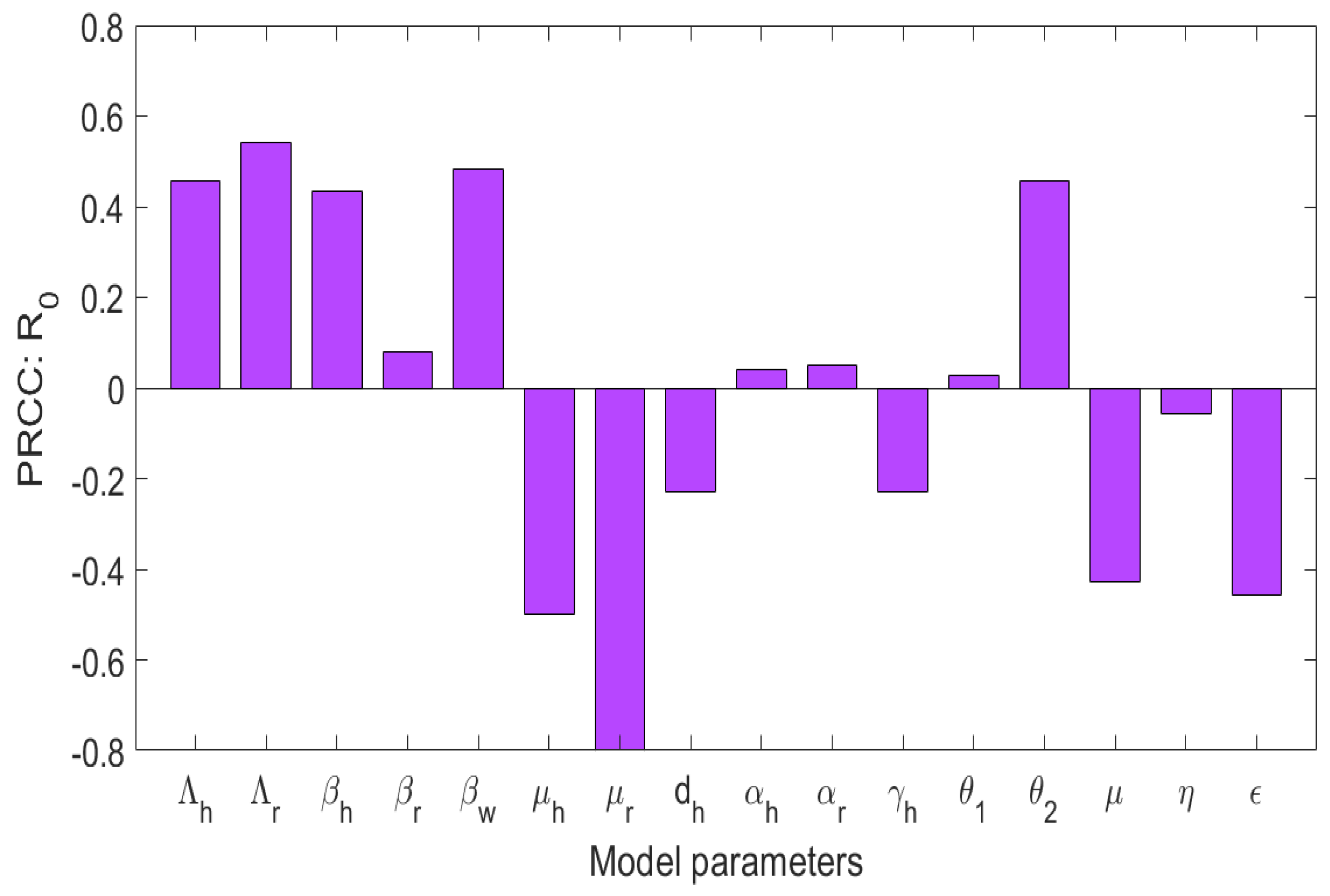
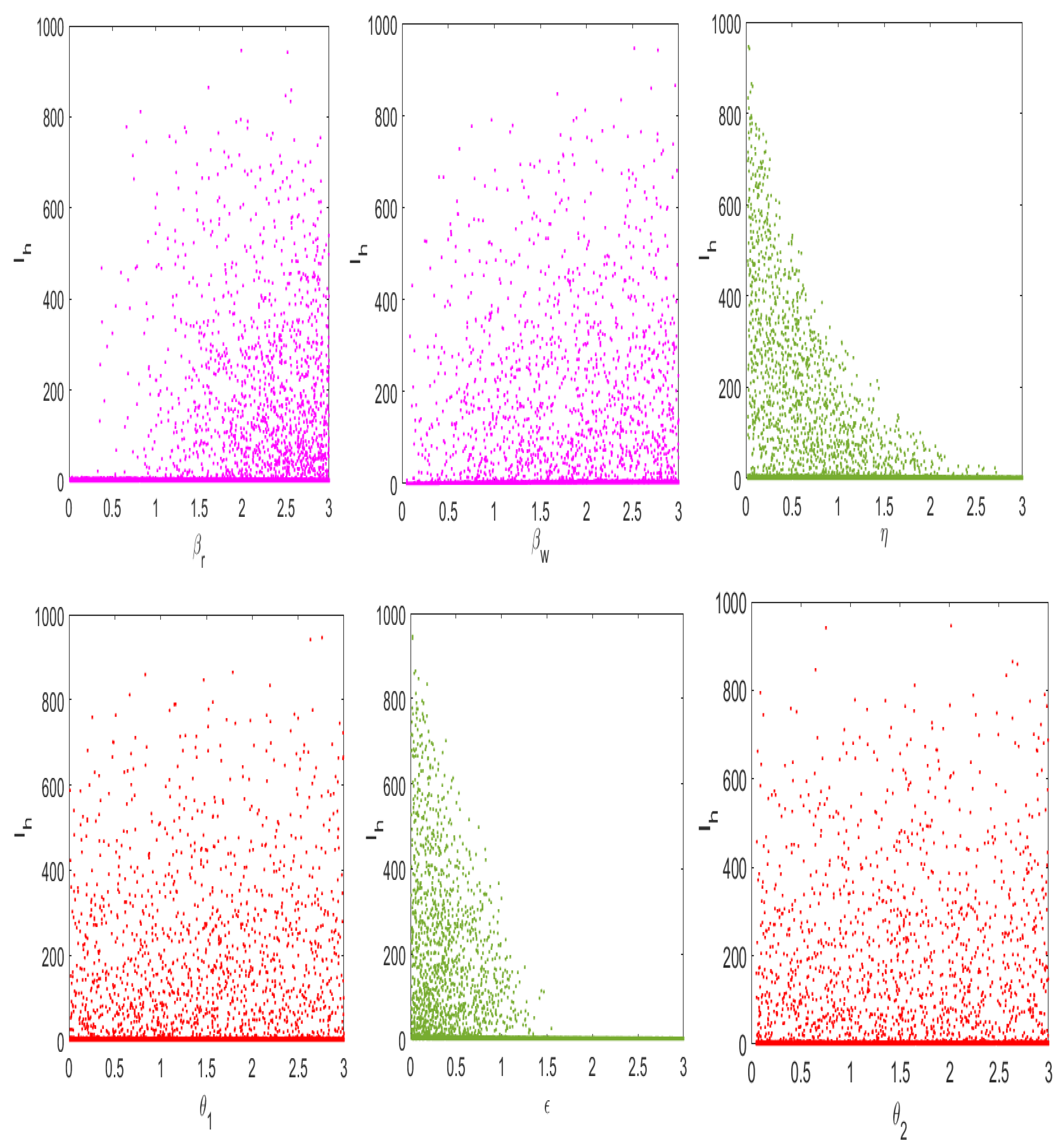
5.2. The Sensitivity Analysis

In this section, we investigate the sensitivity of the basic reproduction number, ${\mathcal{R}}_0$, to changes in the model parameters using partial rank correlation coefficients (PRCCs). The results are illustrated in Figure 6. Parameters with positive PRCC values are positively correlated with ${\mathcal{R}}_0$, indicating that an increase in their values leads to a rise in disease transmission. These include the recruitment rate of humans (${\mathrm{\Lambda }}_h$), the birth rate of rodents (${\mathrm{\Lambda }}_r$), the transmission rates from the environment and between hosts (${\beta }_h$, ${\beta }_r$, and ${\beta }_w$), the progression rates of rodents and humans from the exposed class to the infectious class (${\alpha }_r$ and ${\alpha }_h$), and the shedding rate of the virus into the environment from infected rodents (${\theta }_2$). These results suggest that increased host population turnover, higher transmission efficiency, and environmental contamination significantly amplify the potential spread of monkeypox. In contrast, parameters with negative PRCC values are negatively correlated with ${\mathcal{R}}_0$, meaning that increasing these parameters results in reduced disease transmission. These include the natural mortality rates of humans and rodents (${\mu }_h$ and ${\mu }_r$), the rate of public health awareness (${\gamma }_h$), the additional human death rate due to the disease ($\eta$), the virus decay rate due to environmental sanitation ($\mu$), and mortality of the virus due to environmental cleanliness ($ϵ$). The strongest negative impact is associated with ${\mu }_r$, $\mu$, and $ϵ$, emphasizing the critical role of rodent control and environmental sanitation in curbing disease spread. In particular, increasing public health education (${\gamma }_h$) significantly reduces ${\mathcal{R}}_0$, highlighting the importance of awareness campaigns in managing the outbreak. These findings highlight the need for integrated intervention strategies that combine rodent control, environmental hygiene, and community-based awareness programs. While targeting the transmission rates directly is effective, sustainable reductions in ${\mathcal{R}}_0$ are more likely to be achieved through improvements in sanitation practices and health education, especially in endemic regions.

The numerical results in Figure 7 demonstrate the relationship between the dynamical behavior of the infected individuals ($I_h$) and key parameters that affect the dynamics of disease in the community. From the numerical results, one can note that increases in the parameters that represent the rate of environmental sanitation and human awareness on monkeypox disease transmission lead to decreases in the number of infected humans in the population. In contrast, one can note that increases in the parameters that represent the rate of disease transmission from human to human, the rate of disease transmission from the environment to humans, the rate of virus shedding into the environment from rodents, and the rate of virus shedding into the environment from infected humans lead to increases in the spread of disease in the population. In particular, we observed that as the rate of insecticide ($ϵ$) and the vector mortality rate (${\mu }_v$) rise above $0.5$, the number of infected humans in the population decreases.

Next, we perform numerical simulations of Latin Hypercube sampling to demonstrate the relationship between ${\mathcal{R}}_0$ and the key parameters which are strongly correlated with it, and the results are presented in Figure 8. We observe that the simulation results in Figure 8 concur with the earlier findings in Figure 7. In particular, one can note that the parameters $\eta$ and $ϵ$ have negative correlations with ${\mathcal{R}}_0$. On the other hand, we observe that whenever the rate of disease transmission and the virus shedding rates from both rodents and humans (both have positive correlations with ${\mathcal{R}}_0$) are increased, the disease persists in the population.

Figure 9 shows contour plots of ${\mathcal{R}}_0$ (a) as a function of human awareness ($ϵ$) and environmental sanitation $\eta$ and (b) as a function of human awareness ($ϵ$) and the shedding rate of the virus into the environment from humans (${\theta }_2$)). Overall, we observe that in the presence of environmental sanitation ($\eta$) along with human awareness ($ϵ$), the magnitude of ${\mathcal{R}}_0$ decreases. The results have implications for policymakers and other stakeholders, who must allocate resources to human awareness campaigns and environmental sanitation.

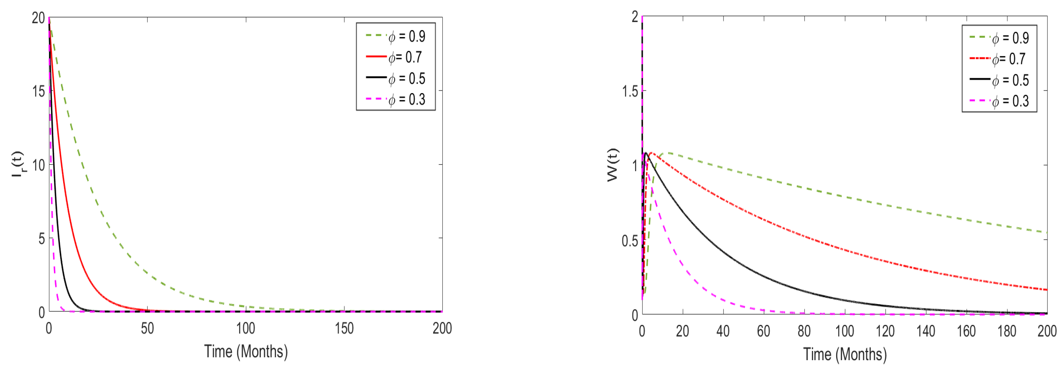
5.3. The Role of Memory Effects on the Disease Dynamics

In this part, we perform a numerical simulation to assess the impact of memory effects on the spread of monkeypox disease. The proposed model (3) is simulated at both ${\mathcal{R}}_0<1$ and ${\mathcal{R}}_0>1$, and the results are presented in Figure 10 and Figure 11, respectively. For the purposes of the numerical simulation, we set the order of derivatives to be ($\varphi =0.3,0.5,0.7,0.9$). From the numerical illustrations, we observe that as the order of the derivatives $\varphi$ decreases from 1 (in particular, when ${\mathcal{R}}_0<1$), the model solutions decrease and converge quickly to a unique equilibrium point (after 20 days), which is the disease-free equilibrium point. On the other hand, when ${\mathcal{R}}_0>1$, the memory effects become strong, and the model solutions converge to a unique point, which is the endemic equilibrium point.

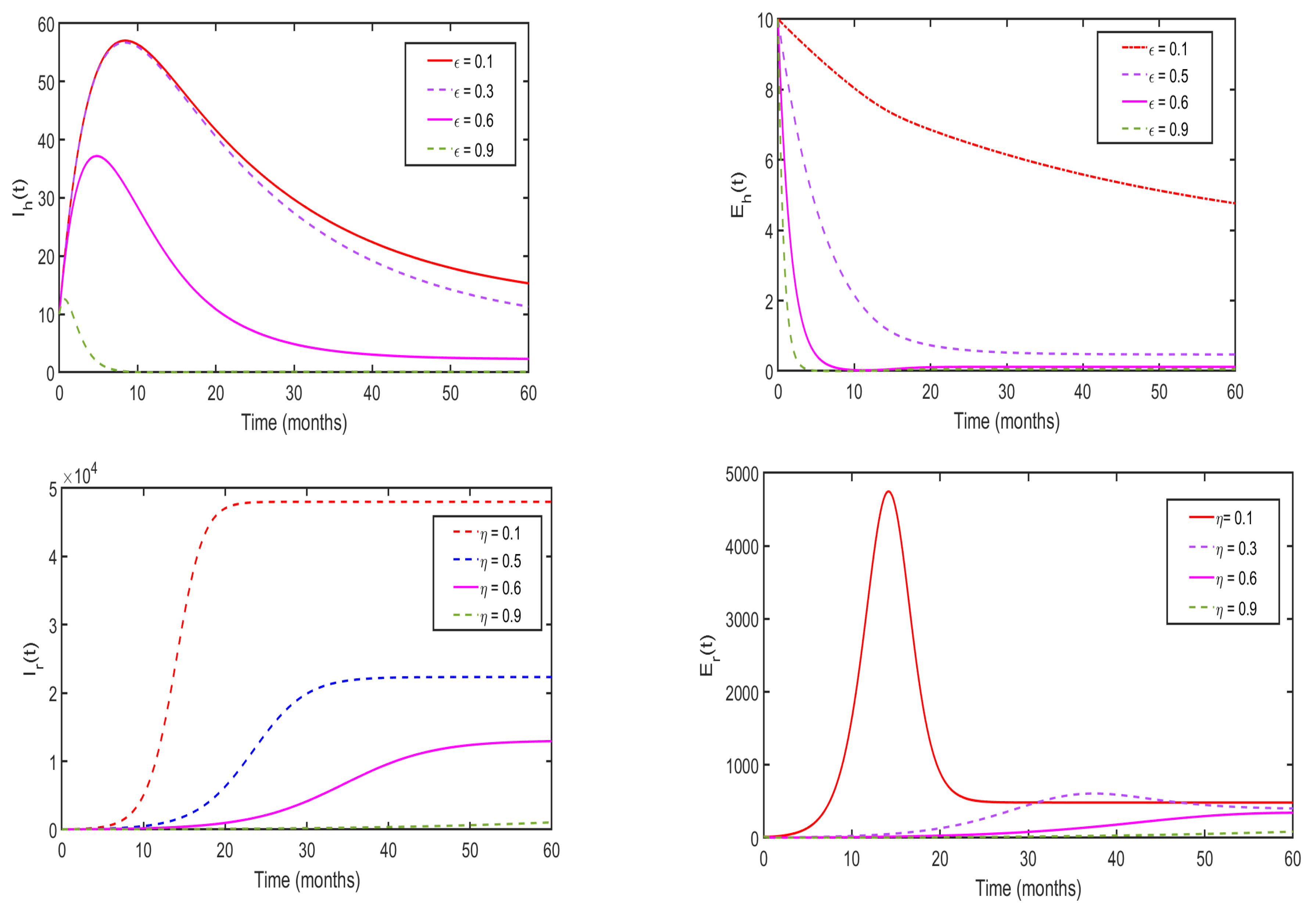
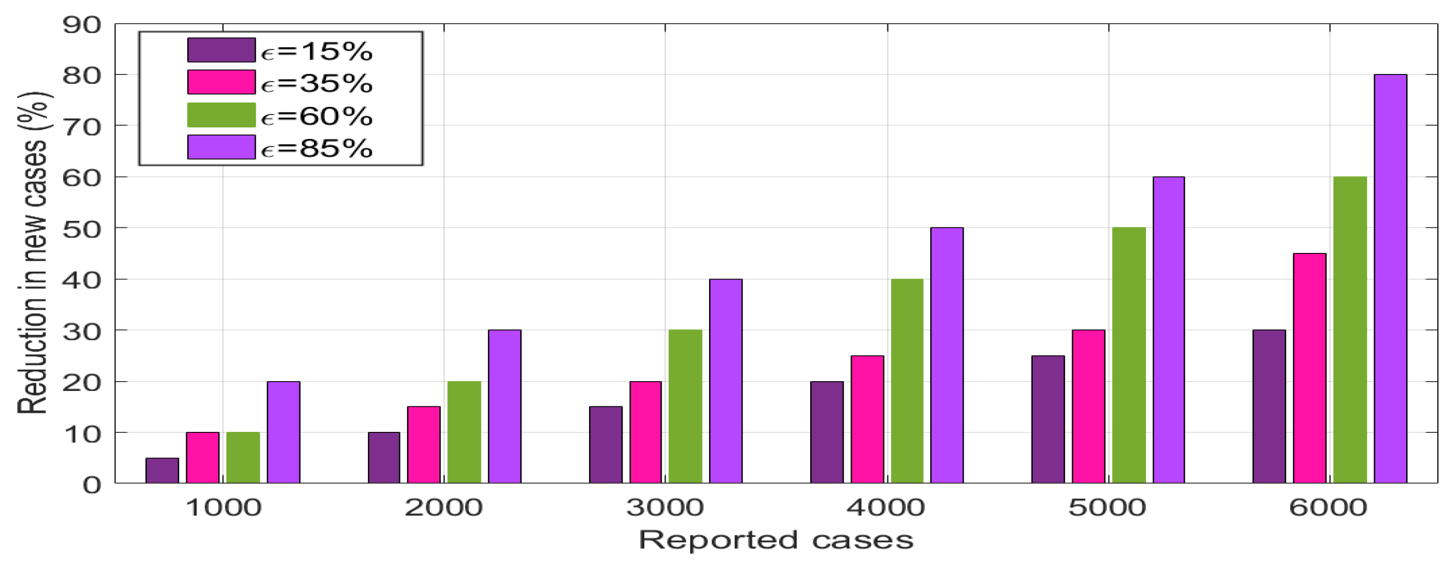
5.4. Effects of Environmental Sanitation and Human Awareness on the Disease Dynamics

Figure 12 shows the effect of environmental sanitation and human awareness on the transmission dynamics of monkeypox. We varied the values of $ϵ$ (top row) and $\eta$ (bottom row) within a reasonable range and used the parameters presented in Table 1 to simulate model system (3). Overall, we observed that the use of environmental sanitation and human awareness simultaneously significantly reduce the spread of monkeypox disease in the community. In addition, we observed that as $ϵ=0.1$ and $\eta =0.1$$({\mathcal{R}}_0>1)$, disease persists in the population, and when $ϵ=0.9$ and $\eta =0.9$, the magnitude of ${\mathcal{R}}_0$ is less than one unit. Thus, the disease dies in the population. Furthermore, we performed a numerical simulation of system (3) to investigate the effects of human awareness on the reduction in newly reported cases of malaria monkeypox disease, and the results are presented in Figure 13. Overall, we observe that implementing health education campaigns to a level of $85\%$ leads to a greater reduction in reported cases of monkeypox disease in the population.

6. Concluding Remarks

In this paper, we proposed and studied a fractional-order model for capturing the transmission dynamics of the monkeypox virus, incorporating the effects of human awareness and environmental sanitation as key intervention strategies. We computed the disease-free equilibrium and computed the threshold quantity number $\left({\mathcal{R}}_0\right)$ using the next-generation matrix approach. The comprehensive sensitivity analysis based on the PRCCs revealed that increasing the parameters with negative sensitivity indices (e.g., awareness and sanitation rates) led to a reduction in $\left({\mathcal{R}}_0\right)$, promoting disease elimination. In contrast, increasing parameters with positive indices sustained or exacerbated transmission, indicating their critical role in disease persistence. To validate the model, we calibrated it using 29 months of monkeypox case data from the Democratic Republic of Congo. The fractional-order model ($\varphi =0.5$) provided a better fit to the real data compared to that of the classical integer-order model ($\varphi =1$), highlighting the importance of incorporating memory effects into modeling real-world disease systems. These findings are consistent with reports from the World Health Organization [54] and the Centers for Disease Control and Prevention [55], which emphasize that behavioral interventions, such as public health awareness campaigns and improved sanitation practices, are critical to controlling Mpox outbreaks. Through numerical simulations at different fractional orders ($\varphi =0.3,0.5,0.7,$ and $0.9$), we observed that lower-derivative orders led to faster convergence to equilibrium states, suggesting that biological systems exhibit stronger memory and damping effects when the derivative order is small. Moreover, the intervention simulations demonstrated that achieving high levels of human awareness and environmental sanitation (each $\ge 90\%$) could significantly reduce the disease burden and potentially lead to its eradication. These findings highlight the synergistic impact of behavioral and environmental strategies on disease control, supporting the current public health recommendations.

This study was subject to several limitations. First, some parameter values, such as the shedding rates and intervention effect sizes, were either drawn from the literature or estimated via model fitting due to the limited available data. Second, the environmental compartment in the model is simplified and may not fully capture the complex dynamics of pathogen survival and decay in real-world settings (we opted for something simpler). Third, the model fitting is based on a single dataset without external validation or cross-validation techniques, which may limit its generalizability. Additionally, the model assumes homogeneous mixing in the population and does not account for spatial or demographic heterogeneity. Finally, while the simulations provide valuable insights, they are not exhaustive and do not explore the uncertainty in the model outcomes, such as through stochastic simulations or confidence intervals.

Future extensions of the model may include animal and human migration, which can influence spatial spread, as well as the differentiation of wild and domestic animal reservoirs, to understand zoophytic transmission in diverse ecological settings better. Overall, the proposed framework offers a robust and realistic tool for informing monkeypox control strategies, particularly in resource-limited and high-risk regions.

References

1. Hatami, H.; Jamshidi, P.; Arbabi, M.; Safavi-Naini, S.A.A.; Farokh, P.; Izadi-Jorshari, G.; Mohammadzadeh, B.; Nasiri, M.J.; Zandi, M.; Nayebzade, A. Demographic, epidemiologic, and clinical characteristics of human monkeypox disease pre-and post-2022 outbreaks: A systematic review and meta-analysis. Biomedicines 2023, 11, 957. [Google Scholar] [CrossRef] [PubMed]
2. Banuet-Martinez, M.; Yang, Y.; Jafari, B.; Kaur, A.; Butt, Z.A.; Chen, H.H.; Yanushkevich, S.; Moyles, I.R.; Heffernan, J.M.; Korosec, C.S. Monkeypox: A review of epidemiological modelling studies and how modelling has led to mechanistic insigh. Epidemiol. Infect. 2023, 151, e121. [Google Scholar] [CrossRef] [PubMed]
3. El-Mesady, A.; Elsonbaty, A.; Adel, W. On nonlinear dynamics of a fractional order monkeypox virus model. Chaos Solitons Fractals 2022, 164, 112716. [Google Scholar] [CrossRef] [PubMed]
4. Farman, M.; Akgül, A.; Garg, H.; Baleanu, D.; Hincal, E.; Shahzeen, S. Mathematical analysis and dynamical transmission of monkeypox virus model with fractional operator. Expert Syst. 2025, 42, e13475. [Google Scholar] [CrossRef]
5. Alakunle, E.; Moens, U.; Nchinda, G.; Okeke Malachy, I. Monkeypox virus in Nigeria: Infection biology, epidemiology, and evolution. Viruses 2020, 12, 1257. [Google Scholar] [CrossRef]
6. Mandja, B.-A.M.; Brembilla, A.; Handschumacher, P.; Bompangue, D.; Gonzalez, J.-P.; Muyembe, J.-J.; Mauny, F. Temporal and spatial dynamics of monkeypox in Democratic Republic of Congo, 2000–2015. EcoHealth 2019, 16, 476–487. [Google Scholar] [CrossRef]
7. Ayeh, M.A.; Cofie, K.; Mensah, G.S.; Amo-Kodieh, F.; Kyeremeh, P. Monkeypox Infection: Risk Assessment and Clinical Outcomes Among Immunocompromised Populations in Sub-Saharan Africa:: A Systematic Review and Meta-analysis. Ghana J. Nurs. Midwifery 2024, 1, 107–124. [Google Scholar] [CrossRef]
8. Di Gennaro, F.; Veronese, N.; Marotta, C.; Shin, J.I.; Koyanagi, A.; Silenzi, A.; Antunes, M.; Saracino, A.; Bavaro, D.F.; Soysal, P. Human monkeypox: A comprehensive narrative review and analysis of the public health implications. Microorganisms 2022, 10, 1633. [Google Scholar] [CrossRef]
9. Chaix, E.; Boni, M.; Guillier, L.; Bertagnoli, S.; Mailles, A.; Collignon, C.; Kooh, P.; Ferraris, O.; Martin-Latil, S.; Manuguerra, J.-C. Risk of Monkeypox virus (MPXV) transmission through the handling and consumption of food. Microb. Risk Anal. 2022, 22, 100237. [Google Scholar] [CrossRef]
10. Lusekelo, E.; Helikumi, M.; Kuznetsov, D.; Mushayabasa, S. Dynamic modelling and optimal control analysis of a fractional order chikungunya disease model with temperature effects. Results Control Optim. 2023, 10, 100206. [Google Scholar] [CrossRef]
11. Mckenzie, H.W.; Jin, Y.; Jacobsen, J.; Lewis Mark, A. R_0 analysis of a spatiotemporal model for a stream population. SIAM J. Appl. Dyn. Syst. 2012, 11, 567–596. [Google Scholar] [CrossRef]
12. Peter, O.J.; Abidemi, A.; Ojo, M.M.; Ayoola Tawakalt, A. Mathematical model and analysis of monkeypox with control strategies. Eur. Phys. J. Plus 2023, 138, 242. [Google Scholar] [CrossRef]
13. Peter, O.J.; Madubueze, C.E.; Ojo, M.M.; Oguntolu, F.A.; Ayoola Tawakalt, A. Modeling and optimal control of monkeypox with cost-effective strategies. Model. Earth Syst. Environ. 2023, 9, 1989–2007. [Google Scholar] [CrossRef]
14. El Mansouri, A.; Smouni, I.; Khajji, B.; Labzai, A.; Belam, M. Mathematical modeling and optimal control strategy for the monkeypox epidemic. Math. Model. Comput. 2023, 10, 944–955. [Google Scholar] [CrossRef]
15. Okongo, W.; Okelo Abonyo, J.; Kioi, D.; Moore, S.E.; Nnaemeka Aguegboh, S. Mathematical modeling and optimal control analysis of Monkeypox virus in contaminated environment. Model. Earth Syst. Environ. 2024, 10, 3969–3994. [Google Scholar] [CrossRef]
16. Soni, K.; Sinha, A.K. Modeling and stability analysis of the transmission dynamics of monkeypox with control intervention. Partial Differ. Equations Appl. Math. 2024, 10, 100730. [Google Scholar] [CrossRef]
17. Musafir, R.R.; Suryanto, A.; Darti, I. Optimal control of a fractional-order monkeypox epidemic model with vaccination and rodents culling. Results Control Optim. 2024, 14, 100381. [Google Scholar] [CrossRef]
18. Peter, O.J.; Kumar, S.; Kumari, N.; Oguntolu, F.A.; Oshinubi, K.; Musa, R. Transmission dynamics of Monkeypox virus: A mathematical modelling approach. Model. Earth Syst. Environ. 2022, 8, 3423–3434. [Google Scholar] [CrossRef]
19. Adepoju, O.A.; Ibrahim, H.O. An optimal control model for monkeypox transmission dynamics with vaccination and immunity loss following recovery. Healthc. Anal. 2024, 6, 100355. [Google Scholar] [CrossRef]
20. Alshehri, A.; Ullah, S. Optimal control analysis of Monkeypox disease with the impact of environmental transmission. Aims Math. 2023, 8, 16926–16960. [Google Scholar] [CrossRef]
21. Rashid, S.; Bariq, A.; Ali, I.; Sultana, S.; Siddiqa, A.; Elagan Sayed, K. Dynamic analysis and optimal control of a hybrid fractional monkeypox disease model in terms of external factors. Sci. Rep. 2025, 15, 2944. [Google Scholar] [CrossRef]
22. Adel, W.; Elsonbaty, A.; Aldurayhim, A.; El-Mesady, A. Investigating the dynamics of a novel fractional-order monkeypox epidemic model with optimal control. Alex. Eng. J. 2023, 73, 519–542. [Google Scholar] [CrossRef]
23. Musafir, R.R.; Suryanto, A.; Darti, I. Stability analysis of a fractional-order monkeypox epidemic model with quarantine and hospitalization. J. Biosaf. Biosecurity 2024, 6, 34–50. [Google Scholar] [CrossRef]
24. ul Rehman, A.; Singh, R.; Abdeljawad, T.; Okyere, E.; Guran, L. Modeling, analysis and numerical solution to malaria fractional model with temporary immunity and relapse. Adv. Differ. Equ. 2021, 2021, 390. [Google Scholar] [CrossRef]
25. Ahmad, Y.U.; Andrawus, J.; Ado, A.; Maigoro, Y.A.; Yusuf, A.; Althobaiti, S.; Mustapha, U.T. Mathematical modeling and analysis of human-to-human monkeypox virus transmission with post-exposure vaccination. Model. Earth Syst. Environ. 2024, 10, 2711–2731. [Google Scholar] [CrossRef]
26. Yuan, P.; Tan, Y.; Yang, L.; Aruffo, E.; Ogden, N.H.; Bélair, J.; Arino, J.; Heffernan, J.; Watmough, J.; Carabin, H. Modeling vaccination and control strategies for outbreaks of monkeypox at gatherings. Front. Public Health 2022, 10, 1026489. [Google Scholar] [CrossRef] [PubMed]
27. Liu, B.; Farid, S.; Ullah, S.; Altanji, M.; Nawaz, R.; Wondimagegnhu Teklu, S. Mathematical assessment of monkeypox disease with the impact of vaccination using a fractional epidemiological modeling approach. Sci. Rep. 2023, 13, 13550. [Google Scholar] [CrossRef]
28. Addai, E.; Ngungu, M.; Omoloye, M.A.; Marinda, E. Modelling the impact of vaccination and environmental transmission on the dynamics of monkeypox virus under Caputo operator. Math. Biosci. Eng. 2023, 20, 10174–10199. [Google Scholar] [CrossRef]
29. Venkatesh, A.; Manivel, M.; Arunkumar, K.; Prakash Raj, M.; Shyamsunder Purohit, S.D. A fractional mathematical model for vaccinated humans with the impairment of Monkeypox transmission. Eur. Phys. J. Spec. Top. 2024, 1–21. [Google Scholar] [CrossRef]
30. Alqahtani, R.T.; Musa, S.S.; Inc, M. Modeling the role of public health intervention measures in halting the transmission of monkeypox virus. AIMS Math. 2023, 8, 14142–14166. [Google Scholar] [CrossRef]
31. Biswas, A.S.; Aslam, B.H.; Tiwari, P.K. Mathematical modeling of a novel fractional-order monkeypox model using the Atangana–Baleanu derivative. Phys. Fluids 2023, 35, 11. [Google Scholar] [CrossRef]
32. Yaga, S.J. Modeling Monkeypox Epidemics: Thresholds, Temporal Dynamics, and Waning Immunity from Smallpox Vaccination. medRxiv 2025. [Google Scholar] [CrossRef]
33. Spath, T.; Brunner-Ziegler, S.; Stamm, T.; Thalhammer, F.; Kundi, M.; Purkhauser, K.; Handisurya, A. Modeling the protective effect of previous compulsory smallpox vaccination against human monkeypox infection: From hypothesis to a worst-case scenario. Int. J. Infect. Dis. 2022, 124, 107–112. [Google Scholar] [CrossRef] [PubMed]
34. Helikumi, M.; Bisaga, T.; Makau, K.A.; Mhlanga, A. Modeling the Impact of Human Awareness and Insecticide Use on Malaria Control: A Fractional-Order Approach. Mathematics 2024, 12, 3607. [Google Scholar] [CrossRef]
35. Helikumi, M.; Mushayabasa, S. Mathematical modeling of trypanosomiasis control strategies in communities where human, cattle and wildlife interact. Anim. Dis. 2023, 3, 25. [Google Scholar] [CrossRef]
36. Khan, A.; Sabbar, Y.; Din, A. Stochastic modeling of the Monkeypox 2022 epidemic with cross-infection hypothesis in a highly disturbed environment. Math. Biosci. Eng. 2022, 19, 13560–13581. [Google Scholar] [CrossRef]
37. Brand, S.P.C.; Cavallaro, M.; Cumming, F.; Turner, C.; Florence, I.; Blomquist, P.; Hilton, J.; Guzman-Rincon, L.M.; House, T.; Nokes, D.J. The role of vaccination and public awareness in forecasts of Mpox incidence in the United Kingdom. Nat. Commun. 2023, 14, 4100. [Google Scholar] [CrossRef]
38. Rakkiyappan, R.; Latha, V.P.; Rihan, F.A. A Fractional-Order Model for Zika Virus Infection with Multiple Delays. Complexity 2019, 1, 4178073. [Google Scholar] [CrossRef]
39. Ghanbari, B.; Atangana, A. A new application of fractional Atangana–Baleanu derivatives: Designing ABC-fractional masks in image processing. Phys. A Stat. Mech. Its Appl. 2020, 542, 123516. [Google Scholar] [CrossRef]
40. Batiha, I.M.; Abubaker, A.A.; Jebril, I.H.; Al-Shaikh, S.B.; Matarneh, K.; Almuzini, M. A Mathematical Study on a Fractional-Order SEIR Mpox Model: Analysis and Vaccination Influence. Algorithms 2023, 16, 418. [Google Scholar] [CrossRef]
41. Nisar, K.S.; Farman, M.; Abdel-Aty, M.; Ravichandran, C. A review of fractional order epidemic models for life sciences problems: Past, present and future. Alex. Eng. J. 2024, 95, 283–305. [Google Scholar] [CrossRef]
42. Lusekelo, E.; Helikumi, M.; Kuznetsov, D.; Mushayabasa, S. Quantifying the effects of temperature and predation on the growth of Aedes mosquito population. Model. Earth Syst. Environ. 2023, 9, 3193–3206. [Google Scholar] [CrossRef]
43. Helikumi, M.; Lolika Paride, O. Global dynamics of fractional-order model for malaria disease transmission. Asian Res. J. Math. 2022, 18, 82–110. [Google Scholar] [CrossRef]
44. Podlubny, I. Fractional Differential Equations; Academic Press: San Dieg, CA, USA, 1999. [Google Scholar]
45. Delavari, H.; Baleanu, D.; Sadati, J. Stability analysis of Caputo fractional-order nonlinear systems revisited. Nonlinear Dyn. 2012, 67, 2433–2439. [Google Scholar] [CrossRef]
46. Molla, J.; Sekkak, I.; Mundo Ortiz, A.; Moyles, I.; Nasri, B. Mathematical modeling of mpox: A scoping review. ONE Health 2023, 16, 100540. [Google Scholar] [CrossRef] [PubMed] [PubMed Central]
47. Vargas-De-León, C. Volterra-type Lyapunov functions for fractional-order epidemic systems. Commun. Nonlinear Sci. Numer. Simul. 2015, 24, 75–85. [Google Scholar] [CrossRef]
48. Caputo, M. Linear models of dissipation whose Q is almost frequency independent, Part II. Geophys. J. R. Astr. Soc. 1967, 13, 529–539, Reprinted in Fract. Calc. Appl. Anal. 2008, 11, 4–14. [Google Scholar] [CrossRef]
49. Diethelm, K. The Analysis of Fractional Differential Equations: An Application-Oriented Exposition Using Differential Operators of Caputo Type; Springer: Berlin/Heidelberg, Germany, 2010; p. 247. [Google Scholar]
50. van-den Driessche, P.; Watmough, J. Reproduction number and sub-threshold endemic equilibria for compartment models of disease transmission. Math. Biosci. 2002, 180, 29–48. [Google Scholar] [CrossRef]
51. Shuai, Z.; Heesterbeek, J.A.P.; van den Driessche, P. Extending the type reproduction number to infectious disease control targeting contact between types. J. Math. Biol. 2013, 67, 1067–1082. [Google Scholar] [CrossRef]
52. LaSalle, J.P. The Stability of Dynamical Systems; SIAM: Philadelphia, PA, USA, 1976. [Google Scholar]
53. Bhunu, C.P.; Mushayabasa, S. Modelling the transmission dynamics of pox-like infections. IAENG Int. J. 2011, 41, 141–149. [Google Scholar]
54. World Health Organization (WHO). Monkeypox: Public Health Advice for Gay, Bisexual and Other Men Who Have Sex with Men; World Health Organization: Geneva, Switzerland, 2022; Available online: https://www.who.int/news-room/questions-and-answers/item/monkeypox (accessed on 25 April 2025).
55. Centers for Disease Control and Prevention (CDC). Preventing Mpox; Centers for Disease Control and Prevention: Atlanta, GA, USA, 2024. Available online: https://www.cdc.gov/mpox/prevention/index.html (accessed on 25 April 2025).
Figure 1. The transmission cycle of monkeypox disease’s dynamics, illustrating interactions between humans, rodents, and environmental reservoirs. The arrows represent pathways of transmission, including human-to-human contact, zoonotic transmission from rodents, and infection via contaminated environments [9].
Fractalfract 09 00356 g001
Figure 2. A model flowchart illustrating the dynamics of Mpox disease transmission. The red arrows represent infection of susceptible humans and rodents due to exposure to the contaminated environment. Blue arrows show the progression of humans through the disease stages (from susceptible to exposed, exposed to infectious, and infectious to recovered), as well as the shedding of the virus by infectious humans into the environment. Pink arrows illustrate the progression of rodents through their disease stages (from susceptible to exposed to infectious) and the shedding of the virus by infectious rodents into the environment.
Fractalfract 09 00356 g002
Figure 3. Number of reported disease cases over 29 months in Democratic Republic of Congo.
Fractalfract 09 00356 g003
Figure 4. (a) Model fit versus reported monkeypox cases for ϕ = 0.5 (fractional-order model) with an RMS = 0.001721 and ϕ = 1 (integer-order model) with an RMS = 0.5208, showing that the fractional model provides a closer fit to the data. (b) Sum of squared errors for cumulative cases (SSEC) plotted against different derivative orders, demonstrating that fractional orders yield smaller errors compared to those of the classical integer-order model.
Fractalfract 09 00356 g004
Figure 5. (a) Residual versus time series plot, showing that the residuals are scattered randomly around zero, indicating the good fit of the model over time. (b) A leverage versus residual plot showing that most points have low leverage and small residuals, suggesting no influential data points affecting the epidemiological model predictions.
Fractalfract 09 00356 g005
Figure 6. A global sensitivity analysis of R 0 to the model parameters.
Fractalfract 09 00356 g006
Figure 7. Numerical results of the sensitivity analysis of system (3) on ( I h ) to the model parameters.
Fractalfract 09 00356 g007
Figure 8. Global sensitivity analysis of R 0 to the model parameters using Latin Hypercube sampling.
Fractalfract 09 00356 g008
Figure 9. Contour plots of R 0 (a) as a function of human awareness ( ϵ ) and environmental sanitation η and (b) as a function of human awareness ( ϵ ) and the shedding rate of the virus into the environment from humans ( θ 2 ).
Fractalfract 09 00356 g009
Figure 10. Numerical results of the model system (3) when R 0 < 1 ; the order of derivatives was set to ϕ = 0.1 , 0.3 , 0.5 , 0.7 .
Fractalfract 09 00356 g010aFractalfract 09 00356 g010b
Figure 11. Numerical simulation of the proposed system (3) when R 0 > 1 and the order of derivatives was assumed to be ϕ = 0.1 , 0.3 , 0.5 , 0.7 .
Fractalfract 09 00356 g011
Figure 12. Numerical results of the system (3) for assessing the impact of human awareness on the transmission dynamics of monkeypox.
Fractalfract 09 00356 g012
Figure 13. Numerical results of assessing the impact of human awareness ( ϵ ) on newly generated monkeypox infections.
Fractalfract 09 00356 g013