Dynamical Behavior Analysis of Generalized Chen–Lee–Liu Equation via the Riemann–Hilbert Approach

Abstract

In this paper, we investigate the dynamics of the generalized Chen–Lee–Liu (gCLL) equation utilizing the Riemann–Hilbert method to derive its $\mathit{N}$-soliton solution. We incorporate a self-steepening term and a Kerr nonlinear term to characterize nonlinear light propagation in optical fibers based on the Chen–Lee–Liu (CLL) equation more accurately. The Riemann–Hilbert problem is addressed through spectral analysis derived from the Lax pair formulation, resulting in an $\mathit{N}$-soliton solution for a reflectance-less system. We also present explicit formulas for solutions involving one and two solitons, thereby providing theoretical support for stable long-distance signal transmission in optical fiber communication. Furthermore, by adjusting parameters and conducting comparative analyses, we generate three-dimensional soliton images that warrant further exploration. The stability of soliton solutions in optical fibers offers novel insights into the intricate propagation behavior of light pulses, and it is crucial for maintaining the integrity of communication signals.

1. Introduction

The following Chen–Lee–Liu (CLL) equation,

$$\begin{array}{c}\hfill \mathrm{i}{u}_t+u_{xx}-\mathrm{i}{\left|u\right|}^2{u}_x=0,\end{array}$$

(1)

with ${\mathrm{i}}^2=-1$, is recognized as a well-known integrable system in mathematics and physics [1]. Since it may be produced from the nonlinear Schrödinger (NLS) equation using the bi-Hamiltonian method [2], it is also known as the derivative nonlinear Schrödinger II (DNLS II) equation [3]. There are also two further variants of derivative NLS equations [4,5]. One of them is the KN or DNLS I equation given by

$$\begin{array}{c}\hfill \mathrm{i}{u}_t+u_{xx}+\mathrm{i}{\left({\left|u\right|}^{2}u\right)}_x=0,\end{array}$$

and the other is the DNLS III equation, often known as the Gerdjikov–Ivanov (GI) equation [6],

$$\begin{array}{c}\mathrm{i}{u}_t+u_{xx}-\mathrm{i}{u}^2{u}^{*}+{\displaystyle \frac{1}{2}}\left({\left|u\right|}^{4}u\right)=0,\end{array}$$

where the symbol * denotes the complex conjugate.

The observation of plasma lattice vibration patterns and the simulation-based generation and control of optical soliton pulses are two applications of the DNLS-type equations in plasma physics and nonlinear optics fibers [7]. The Chen–Lee–Liu (CLL) Equation (1) is a crucial tool for understanding the nonlinear propagation process of optical pulses in optical fibers. However, as the field of ultra-short and high-power optical pulse research develops, the CLL Equation (1) is no longer sufficient to precisely characterize the propagation properties of optical pulses in specific situations [8]. In order to overcome this limitation, we investigate the propagation of an optical pulse inside a monomode fiber, which is described by the generalized Chen–Lee–Liu (gCLL) equation [9]:

$$\begin{array}{c}\mathrm{i}{u}_t+{\displaystyle \frac{1}{2}}{u}_{xx}-{\left|u\right|}^{2}u+\mathrm{i}\delta {\left|u\right|}^2{u}_x=0,\end{array}$$

(2)

where parameter $\delta >0$ is typically linked to the phenomenon of self-steepening [10]. We incorporated a self-steepening term and a Kerr nonlinear term that has a significant impact on the transmission of high-intensity optical pulses by modifying the group velocity and pulse shape. The gCLL Equation (2) can accurately capture the dynamic changes in group velocity resulting from variations in pulse intensity [11] with this modification. This enhancement improves our ability to predict and evaluate the optical pulse propagation behavior in optical fibers more precisely. Furthermore, this equation is utilized for studying modulated wave dynamics of waves traveling through a single nonlinear transmission network, with potentially valuable implications [12].

Several scientific studies have been conducted on the CLL Equation (1). It has been studied using the Laplace–Adomian decomposition method [13], the inverse scattering transform [14], the Riemann–Hilbert method [15], and other methods [16,17,18]. At present, there are few studies on gCLL Equation (2), including applying Lie symmetries to determine the algebraic solution [9], applying Whitham modulation theory to solve the Riemann problem [11], applying numerical calculation to find exact solution [19], etc. However, the soliton solution of the gCLL Equation (2) and its stability have not been studied.

The soliton solution represents a class of localized traveling-wave solutions characterized by a strict mathematical definition within nonlinear integrable systems. Its fundamental feature lies in the precise balance between nonlinearity and dispersion effects, which enables the solution to maintain lasting stability in waveform, velocity, and amplitude during propagation. Furthermore, it exhibits complete elastic scattering properties when colliding with other solitons; only a phase shift occurs without altering its dynamic parameters [20,21,22]. The $\mathit{N}$-soliton solution, as an exact solution of the system containing $\mathit{N}$ interacting soliton components, can be constructed through rigorous mathematical methods such as the inverse scattering transform (IST) [23], Hirota’s bilinear method [24], Darboux transformation [25], Bäcklund transformation [26], and so on. In the asymptotic limit ($t\to \pm \infty$), it manifests as a linear superposition of $\mathit{N}$-soliton solutions propagating at distinct speeds. Notably, all collision processes adhere to stringent conservation laws regarding kinematic parameters, thereby providing an essential mathematical foundation for assessing the integrability of the system.

Previous studies have demonstrated the applicability of the Riemann–Hilbert method in solving the CLL Equation (1) [7], indicating its potential for solving the gCLL Equation (2). The main purpose of this paper is to research a new integrable extension of the gCLL Equation (2) and to derive its $\mathit{N}$-soliton solution. The soliton solutions existence proves the complete integrability of gCLL equations, which makes it possible to study nonlinear waves by analytical methods. The stability of solitons means that they can maintain the integrity of the signal over long distances, which is particularly important for fiber optic communication technology. In addition, the study of the stability and interaction of soliton solutions has promoted an in-depth understanding of the theory of nonlinear dynamical systems.

The structure of this document is as follows. In Section 2, we will present the Lax pair for the generalized Chen–Lee–Liu Equation (2). Subsequently, we will conduct a spectral analysis leading to the formulation of a Riemann–Hilbert problem on the $\lambda$-plane for this equation. The specific Riemann–Hilbert problems with vanishing scattering coefficients will be solved in Section 3. In Section 4, we will obtain $\mathit{N}$-soliton solutions for the generalized Chen–Lee–Liu Equation (2) and provide partial three-dimensional schematic diagrams illustrating single-soliton and two-soliton solutions. Finally, our conclusions are presented in Section 5.

2. The Riemann–Hilbert Problem

2.1. The Lax Pair of gCLL Equation

Similar to the inverse scattering approach, the Riemann–Hilbert approach is thought of as a direct scattering problem. Formulating the relevant Riemann–Hilbert problem is a step in this process. Consequently, we apply the Jost solution to create the Riemann–Hilbert problem at the outset of this study.

The Lax pairs of the gCLL Equation (2) are matrices defined as follows [11]:

$$\begin{array}{c}\hfill {\Phi }_x(x,t;\lambda )=\mathit{U}(x,t;\lambda )\Phi (x,t;\lambda ),{\Phi }_t(x,t;\lambda )=\mathit{V}(x,t;\lambda )\Phi (x,t;\lambda ).\end{array}$$

(3)

Here,

$$\begin{array}{c}\mathit{U}(x,t;\lambda )=\left(\begin{array}{cc}{U}_{11}& U_{12}\\ U_{21}& -U_{11}\end{array}\right),\mathit{V}(x,t;\lambda )=\left(\begin{array}{cc}{V}_{11}& V_{12}\\ V_{21}& -V_{11}\end{array}\right),\end{array}$$

where

$$\begin{array}{cc}\hfill & U_{11}=-{\displaystyle \frac{\mathrm{i}}{2\delta }}\left({\lambda }^2-{\delta }^2{\left|u\right|}^2+1\right),U_{12}=u\lambda ,U_{21}=-u^{*}\lambda ,\hfill \\ \hfill & V_{11}=-{\displaystyle \frac{\mathrm{i}}{4{\delta }^2}}{\left({\lambda }^2-{\delta }^2{\left|u\right|}^2+1\right)}^2-{\displaystyle \frac{\delta }{4}}(u_x{u}^{*}-u{u}_x^{*})-{\displaystyle \frac{\mathrm{i}}{2}}{\left|u\right|}^2,\hfill \\ \hfill & V_{12}={\displaystyle \frac{1}{2\delta }}\left({\lambda }^2+{\delta }^2{\left|u\right|}^2+1\right)u\lambda -{\displaystyle \frac{\mathrm{i}}{2}}{u}_x\lambda ,\hfill \\ \hfill & V_{21}=-{\displaystyle \frac{1}{2\delta }}\left({\lambda }^2+{\delta }^2{\left|u\right|}^2+1\right)u^{*}\lambda -{\displaystyle \frac{\mathrm{i}}{2}}{u}_x^{*}\lambda ,\hfill \end{array}$$

Subsequently, Equation (2) is demonstrated to be equivalent to the gCLL Equation (2) through a straightforward computation. The standard matrix commutator, in this case, is denoted as $[U,V]=UV-VU$, and illustrated by the use of square brackets.

2.2. Spectral Analysis

The Lax pairs (3) of the gCLL Equation (2) may be obtained by applying the compatibility condition of the following two linear spectrum problems

$$\begin{array}{cc}\hfill {\Phi }_x(x,t;\lambda )=& -{\displaystyle \frac{\mathrm{i}}{2\delta }}({\lambda }^2+1)\sigma \Phi +\left[\lambda Q-{\displaystyle \frac{\mathrm{i}\delta }{2}}{Q}^2\sigma \right]\Phi ,\hfill \\ \hfill {\Phi }_t(x,t;\lambda )=& -{\displaystyle \frac{\mathrm{i}}{4{\delta }^2}}{({\lambda }^2+1)}^2\sigma \Phi +\left\{{\displaystyle \frac{1}{2\delta }}{\lambda }^{3}Q-{\displaystyle \frac{\mathrm{i}}{2}}{\lambda }^2{Q}^2\sigma +\lambda \left[{\displaystyle \frac{\delta }{2}}{Q}^3+{\displaystyle \frac{1}{2\delta }}Q-{\displaystyle \frac{\mathrm{i}}{2}}{Q}_x\sigma \right]-Y\right\}\Phi ,\hfill \end{array}$$

where

$$Q=u{\sigma }_{+}-u^{*}{\sigma }_{-},Y={\displaystyle \frac{\mathrm{i}{\delta }^2}{4}}{Q}^4\sigma +{\displaystyle \frac{\delta }{4}}[Q,Q_x],$$

$$\sigma =\left(\begin{array}{cc}1& 0\\ 0& -1\end{array}\right),{\sigma }_{+}=\left(\begin{array}{cc}0& 1\\ 0& 0\end{array}\right),{\sigma }_{-}=\left(\begin{array}{cc}0& 0\\ 1& 0\end{array}\right).$$

In the discussion that follows, it is found to be more convenient to introduce a new $2\times 2$ matrix spectral function $J=J(x,t;\lambda )$ defined as follows rather than working with the original version of the Lax pair (3)

$$\Phi =Jexp\left[-{\displaystyle \frac{\mathrm{i}}{2\delta }}({\lambda }^2+1)\sigma x-{\displaystyle \frac{\mathrm{i}}{4{\delta }^2}}{({\lambda }^2+1)}^2\sigma t\right].$$

Here, we define

$$\begin{array}{cc}\hfill & \tilde{U}=\lambda Q-{\displaystyle \frac{\mathrm{i}\delta }{2}}{Q}^2\sigma ,\hfill \\ \hfill \tilde{V}={\displaystyle \frac{1}{2\delta }}{\lambda }^{3}Q-{\displaystyle \frac{\mathrm{i}}{2}}& {\lambda }^2{Q}^2\sigma +\lambda \left[{\displaystyle \frac{\delta }{2}}{Q}^3+{\displaystyle \frac{1}{2\delta }}Q-{\displaystyle \frac{\mathrm{i}}{2}}{Q}_x\sigma \right]-Y.\hfill \end{array}$$

(4)

Then, we obtain the equivalent Lax pair of $J(x,t;\lambda )$

$$J_x+{\displaystyle \frac{\mathrm{i}}{2\delta }}({\lambda }^2+1)[\sigma ,J]=\tilde{U}J,$$

(5)

$$J_t+{\displaystyle \frac{\mathrm{i}}{4{\delta }^2}}{({\lambda }^2+1)}^2[\sigma ,J]=\tilde{V}J,$$

(6)

where $[\sigma ,J]=\sigma J-J\sigma$.

We now build two $2\times 2$ matrix Jost solutions for the spectrum problem (5) taking into account the direct scattering process, as shown in [27]:

$$J_{\pm }=({\left[J_{\pm }\right]}_1,{\left[J_{\pm }\right]}_2),$$

where ${\left[J_{\pm }\right]}_1$ and ${\left[J_{\pm }\right]}_2$ denote the first and second columns of the matrix $\left[J_{\pm }\right]$, respectively. In other words, both of them are $2\times 1$ column vectors.

Under boundary conditions

$$J_{\pm }\to \mathbb{I},x\to \pm \infty ,$$

(7)

where $\mathbb{I}$ is the $2\times 2$ identity matrix. $\left[J_{\pm }\right]$ are uniquely determined by the Volterra integral equations [28], and the Jost solutions that could be solved are

$$J_{\pm }(x,\lambda )=\mathbb{I}+{\int }_{\pm \infty }^{x}exp\left[{\displaystyle \frac{\mathrm{i}}{2\delta }}({\lambda }^2+1)\sigma (\xi -x)\right]\tilde{U}(\xi ,\lambda )J_{\pm }(\xi ,\lambda )exp\left[{\displaystyle \frac{\mathrm{i}}{2\delta }}({\lambda }^2+1)\sigma (x-\xi )\right]d\xi .$$

The diagonal form of $\sigma$ and the structure of $\tilde{U}$ in (4) allow us to observe that the first column of $J_{\pm }$ contains the exponential factor $exp\left[{\displaystyle \frac{\mathrm{i}}{\delta }}({\lambda }^2+1)(x-\xi )\right]$, while the second column contains the element $exp\left[{\displaystyle \frac{\mathrm{i}}{\delta }}({\lambda }^2+1)(\xi -x)\right]$. This suggests that ${\left[J_{-}\right]}_1$ and ${\left[J_{+}\right]}_2$ are analytic for $\lambda \in C_{+}$ and continuous for $\lambda \in C_{+}\cup \mathbb{R}\cup \mathrm{i}\mathbb{R}$. As an alternative, ${\left[J_{+}\right]}_1$ and ${\left[J_{-}\right]}_2$ are analytic for $\lambda \in C_{-}$ and continuous for $\lambda \in C_{-}\cup \mathbb{R}\cup \mathrm{i}\mathbb{R}$ [29], where

$$\begin{array}{c}\hfill C_{+}=\left\{\lambda |arg\left(\lambda \right)\in \left(0,{\displaystyle \frac{\pi }{2}}\right)\cup \left(\pi ,{\displaystyle \frac{3\pi }{2}}\right)\right\},\end{array}$$

$$\begin{array}{c}\hfill C_{-}=\left\{\lambda |arg\left(\lambda \right)\in \left({\displaystyle \frac{\pi }{2}},\pi \right)\cup \left({\displaystyle \frac{3\pi }{2}},2\pi \right)\right\}.\end{array}$$

Here, we note that $\mathbb{R}\cup \mathrm{i}\mathbb{R}$ denotes the union of real numbers and pure imaginary numbers within the complex plane.

After defining $E=exp\left[-{\displaystyle \frac{\mathrm{i}}{2\delta }}({\lambda }^2+1)\sigma x\right]$, we can easily compute $J_{-}E$ and $J_{+}E$. Since these two solutions to (5) are distinct, they are connected by a scattering matrix $S\left(\lambda \right)$ [29]:

$$J_{-}E=J_{+}ES\left(\lambda \right),\lambda \in \mathbb{R}\cup \mathrm{i}\mathbb{R}.$$

(8)

It can also be written as

$$J_{-}=J_{+}ES\left(\lambda \right)E^{-1},\lambda \in \mathbb{R}\cup \mathrm{i}\mathbb{R}.$$

(9)

From (9), $detS\left(\lambda \right)=1$ is obtained.

The determinants of $J_{\pm }$ are constants for all x, provided that $tr\left(Q\right)=0$ and Abel’s identity are satisfied [30]. Combining (7) with the boundary conditions, we can obtain

$$det{J}_{\pm }=1.$$

Then, for $x\to +\infty$, scattering matrix $S\left(\lambda \right)$ can be given as

$$\begin{array}{cc}\hfill S\left(\lambda \right)& ={\left(s_{ij}\right)}_{2\times 2}=\underset{x\to +\infty }{lim}{E}^{-1}{J}_{-}E\hfill \\ \hfill & =\mathbb{I}+{\int }_{-\infty }^{+\infty }exp\left[{\displaystyle \frac{\mathrm{i}}{2\delta }}({\lambda }^2+1)\sigma \xi \right]\tilde{U}{J}_{-}(\xi ,\lambda )exp\left[-{\displaystyle \frac{\mathrm{i}}{2\delta }}({\lambda }^2+1)\sigma \xi \right]d\xi ,\lambda \in \mathbb{R}\cup \mathrm{i}\mathbb{R}.\hfill \end{array}$$

To obtain the behavior of the Jost solution for a very large $\lambda$, we need to consider the following expansion [31]:

$$J=J_0+{\displaystyle \frac{J_1}{\lambda }}+{\displaystyle \frac{J_2}{{\lambda }^2}}+\mathcal{O}\left({\displaystyle \frac{1}{{\lambda }^3}}\right),\lambda \to \infty .$$

(10)

After comparing the coefficients of $\lambda$ and substituting (10) into the spectral problem (5), it becomes

$$\begin{array}{cc}\hfill & \mathit{O}\left({\lambda }^2\right):{\displaystyle \frac{\mathrm{i}}{2\delta }}[\sigma ,J_0]=0,\hfill \\ \hfill & \mathit{O}\left(\lambda \right):{\displaystyle \frac{\mathrm{i}}{2\delta }}[\sigma ,J_1]=Q{J}_0,\hfill \\ \hfill & \mathit{O}\left(1\right):J_{0x}+{\displaystyle \frac{\mathrm{i}}{2\delta }}[\sigma ,J_0]+{\displaystyle \frac{\mathrm{i}}{2\delta }}[\sigma ,J_2]=Q{J}_1-{\displaystyle \frac{\mathrm{i}\delta }{2}}{Q}^2\sigma J_0.\hfill \end{array}$$

Upon observing the diagonal element of $\mathit{O}\left(1\right)$, we obtain

$${\displaystyle \frac{\mathrm{i}}{2\delta }}[\sigma ,J_1]=Q{J}_0,J_{0x}=0.$$

There exists a solution Q of the gCLL Equation (2), and it can be easily seen that $J_0=\mathbb{I}$, so we have

$${\displaystyle \frac{\mathrm{i}}{2\delta }}[\sigma ,J_1]=Q.$$

To formulate the Riemann–Hilbert problem, it is necessary to establish a new Jost solution for (5) as

$$P_{+}=({\left[J_{-}\right]}_1,{\left[J_{+}\right]}_2)=J_{+}E\left(\begin{array}{cc}{s}_{11}& 0\\ s_{21}& 1\end{array}\right)E^{-1}=J_{+}E{S}_{+}{E}^{-1},$$

which exhibits asymptotic behavior at large $\lambda$ and is analytic for $\lambda \in C_{+}$ as

$$P_{+}\to \mathbb{I},\lambda \in C_{+}\to \infty .$$

The analytic matrix $P_{-}$ in $C_{-}$ is then constructed, taking into account the adjoint scattering equation of (5) [32]:

$$K_x+{\displaystyle \frac{\mathrm{i}}{2\delta }}({\lambda }^2+1)[\sigma ,K]=-K\tilde{U}.$$

(11)

The adjoint Equation (11) and the boundary conditions $J_{\pm }^{-1}\to \mathbb{I}$ as $x\to \pm \infty$ are clearly satisfied by $J_{\pm }^{-1}$. Furthermore, it can be observed that the matrix function ${({\left[J_{-}^{-1}\right]}^1,{\left[J_{+}^{-1}\right]}^2)}^{\mathsf{T}}$ is analytic in $\lambda \in C_{-}$ using a similar approach as before. For convenience, we designate the k-th row vector of $J_{\pm }^{-1}$ as ${\left[J_{\pm }^{-1}\right]}^k$, $k=1,2$. This allows us to define a matrix function as follows

$$P_{-}={({\left[J_{-}^{-1}\right]}^1,{\left[J_{+}^{-1}\right]}^2)}^{\mathsf{T}}=E\left(\begin{array}{cc}{r}_{11}& r_{12}\\ 0& 1\end{array}\right)E^{-1}{J}_{+}^{-1}=E{R}_{+}{E}^{-1}{J}_{+}^{-1},$$

where

$$R\left(\lambda \right)={\left(r_{ij}\right)}_{2\times 2}=S^{-1}\left(\lambda \right).$$

$P_{-}$ exhibits asymptotic behavior and is analytic in $C_{-}$ as

$$P_{-}\to \mathbb{I},\lambda \in C_{-}\to \infty .$$

For each $\lambda \in C_{\pm }$, there exist two analytic matrix functions $P_{\pm }(x,\lambda )$. Furthermore, it has been established that the solution to the gCLL Equation (2) can be obtained by solving a Riemann–Hilbert problem using these two functions as described below [31]:

$$\begin{array}{cc}\hfill P_{-}{P}_{+}=G(x,\lambda )& =E{R}_{+}{S}_{+}{E}^{-1}=E\left(\begin{array}{cc}1& r_{12}\\ s_{21}& 1\end{array}\right)E^{-1}\hfill \\ \hfill & =\left(\begin{array}{cc}1& exp\left[-{\displaystyle \frac{\mathrm{i}}{\delta }}({\lambda }^2+1)x\right]r_{12}\\ exp\left[{\displaystyle \frac{\mathrm{i}}{\delta }}({\lambda }^2+1)x\right]s_{21}& 1\end{array}\right).\hfill \end{array}$$

(12)

We apply the identity $s_{11}{r}_{11}+s_{12}{r}_{21}=1$ in (12). For this specific Riemann–Hilbert problem, the jump matrix is denoted as $G=G(x,\lambda )$ in (12), and the canonical normalizing conditions are: $P_{+}\to \mathbb{I},\lambda \in C_{+}\to +\infty$, and $P_{-}\to \mathbb{I},\lambda \in C_{-}\to -\infty$.

3. Inverse Scattering Transform

The Riemann–Hilbert problem (12) needs to be solved in order to investigate the inverse scattering transformation of (2). It is evident that, generally, the problem (12) does not have a unique solution unless the zeros of $det{P}_{+}$ and $det{P}_{-}$ are specified. The kernel structures at these locations can be found in [31,33,34,35]. To proceed with this examination, we will now consider the potential zeros of $det{P}_{+}$ and $det{P}_{-}$. By recalling the definitions of $P_{+}$ and $P_{-}$, we have

$$\begin{array}{c}\hfill det{P}_{+}\left(\lambda \right)=s_{11}\left(\lambda \right),\lambda \in C_{+},\end{array}$$

(13)

$$\begin{array}{c}\hfill det{P}_{-}\left(\lambda \right)=r_{11}\left(\lambda \right),\lambda \in C_{-}.\end{array}$$

(14)

To obtain these zeros of $P_{\pm }$, we observe the symmetric relationships of Q,

$$\sigma Q\sigma =-Q,Q^{†}=-Q,$$

where the superscript † denotes the Hermitian conjugate. Therefore, we obtain

$$J_{\pm }(x,t,-\lambda )=\sigma J_{\pm }(x,t,\lambda )\sigma ,\mathrm{and}{J}_{\pm }^{†}(x,t,{\lambda }^{*})=J_{\pm }^{-1}(x,t,\lambda ),\lambda \in \mathbb{R}\cup \mathrm{i}\mathbb{R}.$$

There, it follows from (8),

$$S(-\lambda )=\sigma S\left(\lambda \right)\sigma ,\mathrm{and}{S}^{†}\left({\lambda }^{*}\right)=S^{-1}\left(\lambda \right)=R\left(\lambda \right),\lambda \in \mathbb{R}\cup \mathrm{i}\mathbb{R},$$

which gives the following relationships

$$\begin{array}{cc}\hfill s_{11}(-\lambda )=s_{11}\left(\lambda \right),& \lambda \in C_{+},\hfill \\ \hfill -s_{21}(-\lambda )=s_{21}\left(\lambda \right),& \lambda \in \mathbb{R}\cup \mathrm{i}\mathbb{R},\hfill \end{array}$$

(15)

$$\begin{array}{cc}\hfill s_{11}^{*}\left({\lambda }^{*}\right)=r_{11}\left(\lambda \right),& \lambda \in C_{-},\hfill \\ \hfill s_{21}^{*}\left({\lambda }^{*}\right)=r_{21}\left(\lambda \right),& \lambda \in \mathbb{R}\cup \mathrm{i}\mathbb{R}.\hfill \end{array}$$

(16)

Moreover, we can derive the following relationship from the definitions of $P_{+}$ and $P_{-}$:

$$\begin{array}{cc}\hfill P_{+}\left(\lambda \right)=\sigma P_{+}(-\lambda )\sigma & ,\lambda \in C_{+},\hfill \end{array}$$

(17)

$$\begin{array}{cc}\hfill P_{+}^{†}\left({\lambda }^{*}\right)=P_{-}\left(\lambda \right)& ,\lambda \in C_{-}.\hfill \end{array}$$

(18)

From (13)–(16), it can be inferred that if $\lambda$ is a zero of the determinant of $P_{+}$, then ${\lambda }^{*}$ is a zero of the determinant of $P_{-}$, and $-\lambda$ is another zero of the determinant of $P_{+}$. It is assumed that the determinant of $P_{+}$ has $2N$ simple zeros, denoted as ${\lambda }_j(1\le j\le 2N)$, satisfying the condition that ${\lambda }_{N+l}=-{\lambda }_l(l=1,2,\dots ,N)$, and all these zeros are in region $C_{+}$. Simultaneously, the determinant of $P_{-}$ possesses $2N$ simple zeros denoted as ${\widehat{\lambda }}_j$$(1\le j\le 2N)$ in region $C_{-}$. Furthermore, it holds that ${\widehat{\lambda }}_j={\lambda }_j^{*}$ [36,37].

To solve the Riemann–Hilbert problem (12), we define $v_j$ as a non-zero column vector and ${\widehat{v}}_j$ as a non-zero row vector, both satisfying

$$P_{+}\left({\lambda }_j\right)v_j=0,{\widehat{v}}_j{P}_{-}\left({\widehat{\lambda }}_j\right)=0.$$

(19)

From (17)–(19), we can derive the following relationship

$$\begin{array}{cc}\hfill v_j=\sigma v_{j-N},& (N+1\le j\le 2N),\hfill \end{array}$$

(20)

$$\begin{array}{cc}\hfill {\widehat{v}}_j=v_j^{†},& (1\le j\le 2N).\hfill \end{array}$$

(21)

Then, we obtain the vectors $v_j,(1\le j\le N)$. By taking the partial derivative of $P_{+}\left({\lambda }_j\right)v_j=0$ with respect to x and applying (5), we derive

$$P_{+}\left({\lambda }_j\right)(v_{j,x}+{\displaystyle \frac{\mathrm{i}}{2\delta }}({\lambda }_j^2+1)\sigma v_j)=0,(1\le j\le N),$$

$$v_j=exp\left[-{\displaystyle \frac{\mathrm{i}}{2\delta }}({\lambda }^2+1)\sigma x\right]v_{j,0},(1\le j\le N).$$

(22)

So far, we have focused solely on solving the gCLL Equation (2) at a fixed time. In order to find solutions of (2) at any given time, it is necessary to understand the temporal evolutions of the scattering data [38]. Utilizing (6) and (9), along with the rapid decay of u on the boundary, we derive

$$S_t=-{\displaystyle \frac{\mathrm{i}}{4{\delta }^2}}{({\lambda }^2+1)}^2[\sigma ,S].$$

(23)

Equation (23) yields the time evolution of the scattering matrix entries,

$$\begin{array}{cc}\hfill & s_{11,t}=s_{22,t}=0,\hfill \\ \hfill & s_{12}=s_{12}(\lambda ,0)exp\left[-{\displaystyle \frac{\mathrm{i}}{2{\delta }^2}}{({\lambda }^2+1)}^{2}t\right],\hfill \\ \hfill & s_{21}=s_{21}(\lambda ,0)exp\left[{\displaystyle \frac{\mathrm{i}}{2{\delta }^2}}{({\lambda }^2+1)}^{2}t\right].\hfill \end{array}$$

Taking in account (6), we gain

$$v_{j,t}=-{\displaystyle \frac{\mathrm{i}}{4{\delta }^2}}{({\lambda }^2+1)}^2\sigma v_j,{\displaystyle \frac{\mathrm{d}{\lambda }_j}{\mathrm{d}t}}=0.$$

Therefore, $v_{j,0}$ is independent of x.

In this paper, we only consider the RH problem without reflection. As explained in [36,39,40,41], to derive soliton solutions for the gCLL Equation (2), we choose the jump matrix G to be the $2\times 2$ identity matrix. This guarantees that the reflection does not exist in the scattering problem by setting the vanishing coefficient $s_{21}=s_{12}=0$. Thus, the solution to this Riemann–Hilbert problem can be represented as [15,31,33,36]:

$$P_{+}\left(\lambda \right)=\mathbb{I}-\sum _{k=1}^{2N}\sum _{j=1}^{2N}{\displaystyle \frac{v_k{\widehat{v}}_j{\left(M\right)}_{kj}^{-1}}{\lambda -{\widehat{\lambda }}_j}},$$

(24)

$$P_{-}\left(\lambda \right)=\mathbb{I}+\sum _{k=1}^{2N}\sum _{j=1}^{2N}{\displaystyle \frac{v_k{\widehat{v}}_j{\left(M\right)}_{kj}^{-1}}{\lambda -{\lambda }_k}},$$

where M is a $2N\times 2N$ matrix with entries that are

$$m_{kj}={\displaystyle \frac{{\widehat{v}}_k{v}_j}{{\lambda }_j-{\widehat{\lambda }}_k}},1\le k,j\le 2N.$$

(25)

With the assistance of (25), we will restructure the potentials u. In fact, it is necessary to consider the asymptotic expansion of $P_{+}$ as

$$P_{+}=\mathbb{I}+{\displaystyle \frac{P_{+}^{\left(1\right)}}{\lambda }}+{\displaystyle \frac{P_{+}^{\left(2\right)}}{{\lambda }^2}}+\mathcal{O}\left({\displaystyle \frac{1}{{\lambda }^3}}\right),$$

(26)

when $\lambda \to \infty$, from which we derive

$$Q={\displaystyle \frac{\mathrm{i}}{2\delta }}\left[\sigma ,P_{+}^{\left(1\right)}\right].$$

Subsequently, a direct calculation yields the potential function

$$u={\displaystyle \frac{\mathrm{i}}{\delta }}{\left(P_{+}^{\left(1\right)}\right)}_{12},$$

(27)

where ${\left(P_{+}^{\left(1\right)}\right)}_{12}$ denotes the entry in the (1, 2) position of the matrix function $P_{+}^{\left(1\right)}$. Combining (26) with (24), we can derive the function $P_{+}^{\left(1\right)}$ as follows

$$P_{+}^{\left(1\right)}=-\sum _{k=1}^{2N}\sum _{j=1}^{2N}{v}_k{\widehat{v}}_j{\left(M\right)}_{kj}^{-1}.$$

(28)

4. Soliton Solutions

4.1. N-Soliton Solutions

To deduce the solutions for the gCLL Equation (2), it is necessary to derive the temporal evolutions of the scattering data. Combining (20)–(22), we obtain

$$v_j=\left\{\begin{array}{cc}exp\left({\theta }_j\sigma \right)v_{j,0},\hfill & 1\le j\le N,\hfill \\ \sigma exp\left({\theta }_{j-N}\sigma \right)v_{j-N,0},\hfill & N+1\le j\le 2N,\hfill \end{array}\right.$$

(29)

$${\widehat{v}}_j=\left\{\begin{array}{cc}{v}_{j,0}^{†}exp\left({\theta }_j^{*}\sigma \right),\hfill & 1\le j\le N,\hfill \\ v_{j-N,0}^{†}exp\left({\theta }_{j-N}^{*}\sigma \right)\sigma ,\hfill & N+1\le j\le 2N,\hfill \end{array}\right.$$

(30)

where ${\displaystyle {\theta }_j=-\frac{\mathrm{i}}{2\delta }({\lambda }_j^2+1)x-\frac{\mathrm{i}}{4{\delta }^2}{({\lambda }_j^2+1)}^{2}t}$, with ${\lambda }_j\in C_{+}$, and $v_{j,0}$ being complex constant vectors. The complex constant vectors $v_{j,0}$ are then defined as ${({\alpha }_j,{\beta }_j)}^{\mathsf{T}}$, for $(j=1,2,...,N)$. Utilizing (27)–(30), the $\mathit{N}$-soliton solution formula for the gCLL Equation (2) is derived as follows

$$\begin{array}{cc}u={\displaystyle \frac{\mathrm{i}}{\delta }}{\left(P_{+}^{\left(1\right)}\right)}_{12}\hfill & =-{\displaystyle \frac{\mathrm{i}}{\delta }}\sum _{k=1}^N\sum _{j=1}^N{\alpha }_k{\beta }_j^{*}exp\left[{\theta }_k-{\theta }_j^{*}\right]{\left(M^{-1}\right)}_{kj}\hfill \\ \hfill & +{\displaystyle \frac{\mathrm{i}}{\delta }}\sum _{k=1}^N\sum _{j=N+1}^{2N}{\alpha }_k{\beta }_{j-N}^{*}exp\left[{\theta }_k-{\theta }_{j-N}^{*}\right]{\left(M^{-1}\right)}_{kj}\hfill \\ \hfill & -{\displaystyle \frac{\mathrm{i}}{\delta }}\sum _{k=N+1}^{2N}\sum _{j=1}^N{\alpha }_{k-N}{\beta }_j^{*}exp\left[{\theta }_{k-N}-{\theta }_j^{*}\right]{\left(M^{-1}\right)}_{kj}\hfill \\ \hfill & +{\displaystyle \frac{\mathrm{i}}{\delta }}\sum _{k=N+1}^{2N}\sum _{j=N+1}^{2N}{\alpha }_{k-N}{\beta }_{j-N}^{*}exp\left[{\theta }_{k-N}-{\theta }_{j-N}^{*}\right]{\left(M^{-1}\right)}_{kj},\hfill \end{array}$$

(31)

where $M={\left(m_{kj}\right)}_{2N\times 2N}$ is a non-singular matrix with

$$m_{kj}=\left\{\begin{array}{c}{\displaystyle \frac{{\alpha }_k^{*}{\alpha }_{j}exp\left[{\theta }_k^{*}+{\theta }_j\right]+{\beta }_k^{*}{\beta }_{j}exp\left[-{\theta }_k^{*}-{\theta }_j\right]}{{\lambda }_j-{\lambda }_k^{*}},}\hfill \\ 1\le k,j\le N,\hfill \\ {\displaystyle \frac{{\alpha }_k^{*}{\alpha }_{j-N}exp\left[{\theta }_k^{*}+{\theta }_{j-N}\right]-{\beta }_k^{*}{\beta }_{j-N}exp\left[-{\theta }_k^{*}-{\theta }_{j-N}\right]}{-{\lambda }_{j-N}-{\lambda }_k^{*}},}\hfill \\ 1\le k\le N,N+1\le j\le 2N,\hfill \\ {\displaystyle \frac{{\alpha }_{k-N}^{*}{\alpha }_{j}exp\left[{\theta }_{k-N}^{*}+{\theta }_j\right]-{\beta }_{k-N}^{*}{\beta }_{j}exp\left[-{\theta }_{k-N}^{*}-{\theta }_j\right]}{{\lambda }_j+{\lambda }_{k-N}^{*}},}\hfill \\ N+1\le k\le 2N,1\le j\le N,\hfill \\ {\displaystyle \frac{{\alpha }_{k-N}^{*}{\alpha }_{j-N}exp\left[{\theta }_{k-N}^{*}+{\theta }_{j-N}\right]+{\beta }_{k-N}^{*}{\beta }_{j-N}exp\left[-{\theta }_{k-N}^{*}-{\theta }_{j-N}\right]}{-{\lambda }_{j-N}+{\lambda }_{k-N}^{*}},}\hfill \\ N+1\le k,j\le 2N.\hfill \end{array}\right.$$

and ${\displaystyle {\theta }_j=-\frac{\mathrm{i}}{2\delta }({\lambda }_j^2+1)x-\frac{\mathrm{i}}{4{\delta }^2}{({\lambda }_j^2+1)}^{2}t}$, ${\lambda }_j\in C_{+}$, $j=1,2,\dots ,N$.

In order to satisfy the condition ${\lambda }_{N+l}=-{\lambda }_l,(l=1,2,\dots ,N)$, it was postulated that $det{P}_{+}$ has a total of $2N$ simple zeros in $C_{+}$. This hypothesis led to the derivation of the formula for the N-soliton solution (31). According to this assumption, each zero ${\lambda }_j$ possesses a non-zero real component. We will now consider another type of zeros of $det{P}_{+}$ in order to obtain alternative soliton solutions for (2). In this scenario, we assume that each ${\lambda }_j$ is purely imaginary, and that $det{P}_{+}$ has a maximum of N simple zeros in $C_{+}$. Consequently, we denote by ${\widehat{\lambda }}_j={\lambda }_j^{*}$ that $det{P}_{-}$ contains N simple zeros. The column vectors $v_j$ and the row vectors ${\widehat{v}}_j$, which satisfy $P_{+}\left({\lambda }_j\right)v_j=0$, are obtained similarly as (29) and (30). The expressions ${\widehat{v}}_j{P}_{-}\left({\widehat{\lambda }}_j\right)=0$ can be computed in each case as follows

$$v_j=exp\left({\theta }_j\sigma \right)v_{j,0},{\widehat{v}}_j=v_{j,0}^{†}exp\left({\theta }_j^{*}\sigma \right),1\le j\le N,$$

where ${\displaystyle {\theta }_j=-\frac{\mathrm{i}}{2\delta }({\lambda }_j^2+1)x-\frac{\mathrm{i}}{4{\delta }^2}{({\lambda }_j^2+1)}^{2}t}$, and $v_{j,0}={({\alpha }_j,{\beta }_j)}^{\mathsf{T}}$ are complex constant vectors. Then, analogous to the derivation of the $\mathit{N}$-soliton solution (31), another $\mathit{N}$-soliton solution for the gCLL Equation (2) is obtained.

$$u=-{\displaystyle \frac{\mathrm{i}}{\delta }}\sum _{k=1}^N\sum _{j=1}^N{\alpha }_k{\beta }_j^{*}exp\left[{\theta }_k-{\theta }_j^{*}\right]{\left(M^{-1}\right)}_{kj},$$

(32)

where ${\displaystyle m_{kj}={\left(m_{kj}\right)}_{N\times N}=\frac{{\alpha }_k^{*}{\alpha }_{j}exp\left[{\theta }_k^{*}+{\theta }_j\right]+{\beta }_k^{*}{\beta }_{j}exp\left[-{\theta }_k^{*}-{\theta }_j\right]}{{\lambda }_j-{\lambda }_k^{*}}}$, $1\le k,j\le N$.

4.2. Single-Soliton Solutions

The simplest scenario arises when $N=1$ in the formula for the $\mathit{N}$-soliton solution (31). To illustrate the single-soliton solution explicitly, we specifically assume that ${\lambda }_1=a_1+\mathrm{i}{b}_1$, where $(a_1\ne 0,b_1>0)$. As a result, an exact soliton solution of the gCLL Equation (2) is derived from (31):

$$\begin{array}{cc}\hfill u=& -{\displaystyle \frac{\mathrm{i}}{\delta }}{\alpha }_1{\beta }_1^{*}exp\left[{\theta }_1-{\theta }_1^{*}\right]{\displaystyle \frac{m_{22}+m_{12}-m_{21}-m_{11}}{\left|M\right|}},\hfill \end{array}$$

where $M={\left(m_{kj}\right)}_{2\times 2}$ with

$$\begin{array}{cc}\hfill & m_{11}={\displaystyle \frac{{\left|{\alpha }_1\right|}^{2}exp\left[{\theta }_1^{*}+{\theta }_1\right]+{\left|{\beta }_1\right|}^{2}exp\left[-{\theta }_1^{*}-{\theta }_1\right]}{2\mathrm{i}{b}_1}},\hfill \\ & m_{12}={\displaystyle \frac{{\left|{\alpha }_1\right|}^{2}exp\left[{\theta }_1^{*}+{\theta }_1\right]-{\left|{\beta }_1\right|}^{2}exp\left[-{\theta }_1^{*}-{\theta }_1\right]}{-2a_1}},\hfill \\ \hfill & m_{21}={\displaystyle \frac{{\left|{\alpha }_1\right|}^{2}exp\left[{\theta }_1^{*}+{\theta }_1\right]-{\left|{\beta }_1\right|}^{2}exp\left[-{\theta }_1^{*}-{\theta }_1\right]}{2a_1}},\hfill \\ \hfill & m_{22}={\displaystyle \frac{{\left|{\alpha }_1\right|}^{2}exp\left[{\theta }_1^{*}+{\theta }_1\right]+{\left|{\beta }_1\right|}^{2}exp\left[-{\theta }_1^{*}-{\theta }_1\right]}{-2\mathrm{i}{b}_1}},\hfill \end{array}$$

and ${\displaystyle {\theta }_1=-\frac{\mathrm{i}}{2\delta }[{(a_1+\mathrm{i}{b}_1)}^2+1]x-\frac{\mathrm{i}}{4{\delta }^2}{[{(a_1+\mathrm{i}{b}_1)}^2+1]}^{2}t}$, while $m_{11}{m}_{22}-m_{12}{m}_{21}\ne 0$.

Similarly, we can obtain another single-soliton solution from (32). Setting

$${\displaystyle \frac{{\beta }_1{\beta }_1^{*}}{{\alpha }_1{\alpha }_1^{*}}}=e^{-2{\eta }_1},$$

then we obtain

$$u={\displaystyle \frac{b_1{\beta }_1^{*}}{\delta {\alpha }_1^{*}}}exp\left[{\theta }_1-{\theta }_1^{*}+{\eta }_1\right]\mathrm{sech}\left({\theta }_1+{\theta }_1^{*}+{\eta }_1\right).$$

(33)

The propagation characteristics of single-soliton solution u in (33) are shown in Figure 1.

Figure 1. (a) Modulus of the single-soliton solution u in (33) with $a_1=0.5,b_1=1,{\alpha }_1=2\mathrm{i}$, ${\beta }_1=-5\mathrm{i},\delta =1$. (b) Modulus of the single-soliton solution u in (33) with $a_1=1,b_1=1$, ${\alpha }_1=2,{\beta }_1=\mathrm{i},\delta =1$. (c) The soliton along the x-axis with different times in panel (a). (d) The soliton along the x-axis with different times in panel (b).

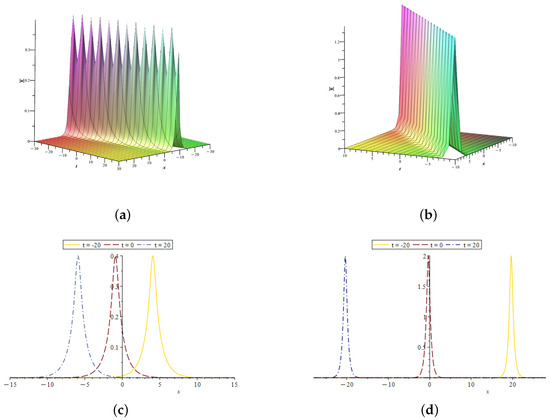
Single-soliton solutions are of great importance in fiber optic communications because they are able to maintain signal integrity over long distances. By analyzing the propagation properties of solitons, we find that there are two types of solitons: periodic collapse solitons and non-singular solitons.

In the case of periodic collapse solitons, their amplitude increases periodically to infinity or decreases to zero. It is a property that may be used in practical applications for specific optical signal modulation techniques. Non-singular solitons maintain constant amplitude and do not collapse during propagation. This stability makes them an ideal information carrier in optical fiber communication.

Figure 1 shows the modulus of two single-soliton solutions. It can be seen from Figure 1a,c that periodic collapse solitons exhibit periodic amplitude changes during propagation. In Figure 1b,d, the amplitude of the non-singular solitons remains stable at different times. The stability characteristics of these two soliton solutions provide a theoretical basis for the design of optical fiber communication systems, especially in the high-power, ultra-short pulse transmission scenarios.

4.3. Double-Soliton Solutions

By taking $N=2$ in (31), we can obtain the double-soliton u

$$\begin{array}{cc}u=\hfill & -{\displaystyle \frac{\mathrm{i}}{\delta }}\sum _{k=1}^2\sum _{j=1}^2{\alpha }_{k}exp\left[{\theta }_k-{\theta }_j^{*}\right]{\left(M^{-1}\right)}_{kj}+{\displaystyle \frac{\mathrm{i}}{\delta }}\sum _{k=1}^2\sum _{j=3}^4{\alpha }_{k}exp\left[{\theta }_k-{\theta }_{j-2}^{*}\right]{\left(M^{-1}\right)}_{kj}\hfill \\ & -{\displaystyle \frac{\mathrm{i}}{\delta }}\sum _{k=3}^4\sum _{j=1}^2{\alpha }_{k-2}exp\left[{\theta }_{k-2}-{\theta }_j^{*}\right]{\left(M^{-1}\right)}_{kj}+{\displaystyle \frac{\mathrm{i}}{\delta }}\sum _{k=3}^4\sum _{j=3}^4{\alpha }_{k-2}exp\left[{\theta }_{k-2}-{\theta }_{j-2}^{*}\right]{\left(M^{-1}\right)}_{kj},\hfill \end{array}$$

where $M={\left(m_{kj}\right)}_{4\times 4}$ with

$$\begin{array}{cc}\hfill & m_{11}={\displaystyle \frac{{\left|{\alpha }_1\right|}^{2}exp\left[{\theta }_1^{*}+{\theta }_1\right]+{\left|{\beta }_1\right|}^{2}exp\left[-{\theta }_1^{*}-{\theta }_1\right]}{{\lambda }_1-{\lambda }_1^{*}}},\hfill \\ \hfill & m_{12}={\displaystyle \frac{{\alpha }_1^{*}{\alpha }_{2}exp\left[{\theta }_1^{*}+{\theta }_2\right]+{\beta }_1^{*}{\beta }_{2}exp\left[-{\theta }_1^{*}-{\theta }_2\right]}{{\lambda }_2-{\lambda }_1^{*}}},\hfill \\ \hfill & m_{13}={\displaystyle \frac{{\left|{\alpha }_1\right|}^{2}exp\left[{\theta }_1^{*}+{\theta }_1\right]-{\left|{\beta }_1\right|}^{2}exp\left[-{\theta }_1^{*}-{\theta }_1\right]}{-{\lambda }_1-{\lambda }_1^{*}}},\hfill \\ \hfill & m_{14}={\displaystyle \frac{{\alpha }_1^{*}{\alpha }_{2}exp\left[{\theta }_2^{*}+{\theta }_1\right]-{\beta }_1^{*}{\beta }_{2}exp\left[-{\theta }_2^{*}-{\theta }_1\right]}{-{\lambda }_2-{\lambda }_1^{*}}},\hfill \\ \hfill & m_{21}={\displaystyle \frac{{\alpha }_2^{*}{\alpha }_{1}exp\left[{\theta }_2^{*}+{\theta }_1\right]+{\beta }_2^{*}{\beta }_{1}exp\left[-{\theta }_2^{*}-{\theta }_1\right]}{{\lambda }_1-{\lambda }_2^{*}}},\hfill \\ \hfill & m_{22}={\displaystyle \frac{{\left|{\alpha }_2\right|}^{2}exp\left[{\theta }_2^{*}+{\theta }_2\right]+{\left|{\beta }_2\right|}^{2}exp\left[-{\theta }_2^{*}-{\theta }_2\right]}{{\lambda }_2-{\lambda }_2^{*}}},\hfill \\ \hfill & m_{23}={\displaystyle \frac{{\alpha }_2^{*}{\alpha }_{1}exp\left[{\theta }_2^{*}+{\theta }_1\right]-{\beta }_2^{*}{\beta }_{1}exp\left[-{\theta }_2^{*}-{\theta }_1\right]}{-{\lambda }_1-{\lambda }_2^{*}}},\hfill \\ \hfill & m_{24}={\displaystyle \frac{{\left|{\alpha }_2\right|}^{2}exp\left[{\theta }_2^{*}+{\theta }_2\right]-{\left|{\beta }_2\right|}^{2}exp\left[-{\theta }_2^{*}-{\theta }_2\right]}{-{\lambda }_2-{\lambda }_2^{*}}},\hfill \\ \hfill & m_{31}={\displaystyle \frac{{\left|{\alpha }_1\right|}^{2}exp\left[{\theta }_1^{*}+{\theta }_1\right]-{\left|{\beta }_1\right|}^{2}exp\left[-{\theta }_1^{*}-{\theta }_1\right]}{{\lambda }_1+{\lambda }_1^{*}}},\hfill \\ \hfill & m_{32}={\displaystyle \frac{{\alpha }_1^{*}{\alpha }_{2}exp\left[{\theta }_1^{*}+{\theta }_2\right]-{\beta }_1^{*}{\beta }_{2}exp\left[-{\theta }_1^{*}-{\theta }_2\right]}{{\lambda }_2+{\lambda }_1^{*}}},\hfill \\ \hfill & m_{33}={\displaystyle \frac{{\left|{\alpha }_1\right|}^{2}exp\left[{\theta }_1^{*}+{\theta }_1\right]+{\left|{\beta }_1\right|}^{2}exp\left[-{\theta }_1^{*}-{\theta }_1\right]}{-{\lambda }_1+{\lambda }_1^{*}}},\hfill \\ \hfill & m_{34}={\displaystyle \frac{{\alpha }_1^{*}{\alpha }_{2}exp\left[{\theta }_1^{*}+{\theta }_2\right]+{\beta }_1^{*}{\beta }_{2}exp\left[-{\theta }_1^{*}-{\theta }_2\right]}{-{\lambda }_2+{\lambda }_1^{*}}},\hfill \\ \hfill & m_{41}={\displaystyle \frac{{\alpha }_2^{*}{\alpha }_{1}exp\left[{\theta }_2^{*}+{\theta }_1\right]-{\beta }_2^{*}{\beta }_{1}exp\left[-{\theta }_2^{*}-{\theta }_1\right]}{{\lambda }_1+{\lambda }_2^{*}}},\hfill \\ \hfill & m_{42}={\displaystyle \frac{{\left|{\alpha }_2\right|}^{2}exp\left[{\theta }_2^{*}+{\theta }_2\right]-{\left|{\beta }_2\right|}^{2}exp\left[-{\theta }_2^{*}-{\theta }_2\right]}{{\lambda }_2+{\lambda }_2^{*}}},\hfill \\ \hfill & m_{43}={\displaystyle \frac{{\alpha }_2^{*}{\alpha }_{1}exp\left[{\theta }_2^{*}+{\theta }_1\right]+{\beta }_2^{*}{\beta }_{1}exp\left[-{\theta }_2^{*}-{\theta }_1\right]}{-{\lambda }_1+{\lambda }_2^{*}}},\hfill \\ \hfill & m_{44}={\displaystyle \frac{{\left|{\alpha }_2\right|}^{2}exp\left[{\theta }_2^{*}+{\theta }_2\right]+{\left|{\beta }_2\right|}^{2}exp\left[-{\theta }_2^{*}-{\theta }_2\right]}{-{\lambda }_2+{\lambda }_2^{*}}},\hfill \end{array}$$

and ${\displaystyle {\theta }_j=-\frac{\mathrm{i}}{2\delta }({\lambda }_j^2+1)x-\frac{\mathrm{i}}{4{\delta }^2}{({\lambda }_j^2+1)}^{2}t}$, while $j=1,2$.

Similarly, when $N=2$ in (32), we can obtain another double-soliton solution u

$$\begin{array}{cc}\hfill u& =-{\displaystyle \frac{\mathrm{i}}{\delta }}\sum _{k=1}^2\sum _{j=1}^2{\alpha }_{k}exp\left[{\theta }_k-{\theta }_j^{*}\right]{\left(M^{-1}\right)}_{kj}\hfill \\ \hfill & =-{\displaystyle \frac{\mathrm{i}}{\delta \left|M\right|}}({\alpha }_1{\beta }_1^{*}{m}_{22}+{\alpha }_1{\beta }_2^{*}{m}_{12}-{\alpha }_2{\beta }_1^{*}{m}_{21}-{\alpha }_2{\beta }_2^{*}{m}_{11}),\hfill \end{array}$$

(34)

where $M={\left(m_{kj}\right)}_{2\times 2}$ with

$$\begin{array}{cc}\hfill & m_{11}={\displaystyle \frac{{\left|{\alpha }_1\right|}^{2}exp\left[{\theta }_1^{*}+{\theta }_1\right]+{\left|{\beta }_1\right|}^{2}exp\left[-{\theta }_1^{*}-{\theta }_1\right]}{{\lambda }_1-{\lambda }_1^{*}}},\hfill \\ \hfill & m_{12}={\displaystyle \frac{{\alpha }_1^{*}{\alpha }_{2}exp\left[{\theta }_1^{*}+{\theta }_2\right]+{\beta }_1^{*}{\beta }_{2}exp\left[-{\theta }_1^{*}-{\theta }_2\right]}{{\lambda }_2-{\lambda }_1^{*}}},\hfill \\ \hfill & m_{21}={\displaystyle \frac{{\alpha }_1{\alpha }_2^{*}exp\left[{\theta }_2^{*}+{\theta }_1\right]+{\beta }_1{\beta }_2^{*}exp\left[-{\theta }_2^{*}-{\theta }_1\right]}{{\lambda }_1-{\lambda }_2^{*}}},\hfill \\ \hfill & m_{22}={\displaystyle \frac{{\left|{\alpha }_2\right|}^{2}exp\left[{\theta }_2^{*}+{\theta }_2\right]+{\left|{\beta }_2\right|}^{2}exp\left[-{\theta }_2^{*}-{\theta }_2\right]}{{\lambda }_2-{\lambda }_2^{*}}},\hfill \end{array}$$

and $m_{11}{m}_{22}-m_{12}{m}_{21}\ne 0$.

Research on the double-soliton solutions of gCLL Equation (2) are mainly divided into two categories: collision of solitons and non-collision of solitons. The propagation characteristics of double-soliton solution u in (34) are shown in Figure 2, Figure 3, Figure 4, Figure 5, Figure 6, Figure 7, Figure 8 and Figure 9.

Figure 2. (a) Modulus of the double-soliton solution via (34) with $\delta =2$, and ${\lambda }_1={\displaystyle \frac{1}{2}}(\sqrt{3}-\mathrm{i}),{\lambda }_2=-{\displaystyle \frac{1}{2}}(\sqrt{3}+\mathrm{i}),{\alpha }_1=-0.2,{\alpha }_2=-0.5,{\beta }_1=-0.1,{\beta }_2=-0.3$. (b) The density distribution of double-soliton solution in panel (a). (c) The double-soliton solution along the x-axis with different times in panel (a).

Figure 3. Moduli graphic of the double-soliton solution (a) and its density distribution (b) with $\delta =2,{\lambda }_1=-1+0.5\mathrm{i},{\lambda }_2=0.5-\mathrm{i},{\alpha }_1=1,{\alpha }_2=\mathrm{i},{\beta }_1=\mathrm{i},{\beta }_2=1$.

Figure 4. Moduli graphics of the double-soliton solution and its density distribution via (34) with $\delta =2$ and (a,b) ${\lambda }_1=1+0.5\mathrm{i},{\lambda }_2=\mathrm{i},{\alpha }_1=1,{\alpha }_2=1,{\beta }_1=1,{\beta }_2=1$; (c,d) ${\lambda }_1=1.5\mathrm{i}$, ${\lambda }_2=1.1\mathrm{i},{\alpha }_1=1,{\alpha }_2=1,{\beta }_1=1,{\beta }_2=1$.

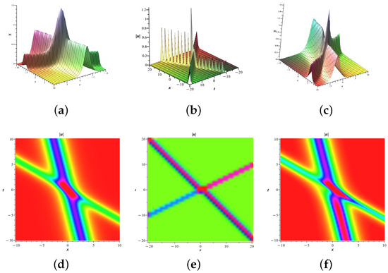
Figure 5. Moduli graphics of the double-soliton solution and its density distribution via (34) with $\delta =2$ and (a,d) ${\lambda }_1=-0.5+\mathrm{i},{\lambda }_2=1-0.5\mathrm{i},{\alpha }_1=1,{\alpha }_2=1,{\beta }_1=1,{\beta }_2=1$; (b,e) ${\lambda }_1=1+2\mathrm{i}$, ${\lambda }_2=1-\mathrm{i},{\alpha }_1={\displaystyle \frac{\sqrt{2}}{2}}(4+\mathrm{i}),{\alpha }_2=2\mathrm{i},{\beta }_1={\displaystyle \frac{\sqrt{2}}{2}}(1-8\mathrm{i}),{\beta }_2=0.5$; (c,f) ${\lambda }_1=-0.5+\mathrm{i}$, ${\lambda }_2=1-0.5\mathrm{i},{\alpha }_1=1,{\alpha }_2=1+\mathrm{i},{\beta }_1=1,{\beta }_2=1$.

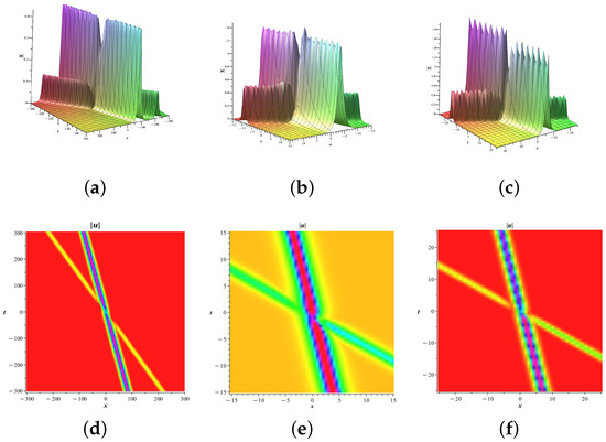
Figure 6. Moduli graphics of the double-soliton solution and its density distribution via (34) with $\delta =2$ and (a,d) ${\lambda }_1=0.7+0.2\mathrm{i},{\lambda }_2=-0.2+0.7\mathrm{i},{\alpha }_1=-\mathrm{i},{\alpha }_2=0.5\mathrm{i},{\beta }_1=\mathrm{i},{\beta }_2=-0.5\mathrm{i}$; (b,e) ${\lambda }_1=1+0.5\mathrm{i},{\lambda }_2=-0.5+\mathrm{i},{\alpha }_1=0.7\mathrm{i},{\alpha }_2=0.7+0.3\mathrm{i},{\beta }_1=0.3\mathrm{i},{\beta }_2=0.3+0.7\mathrm{i}$; (c,f) $1+0.5\mathrm{i},{\lambda }_2=-0.5+\mathrm{i},{\alpha }_1=-\mathrm{i},{\alpha }_2=0.5+0.5\mathrm{i},{\beta }_1=\mathrm{i},{\beta }_2=-0.5\mathrm{i}$.

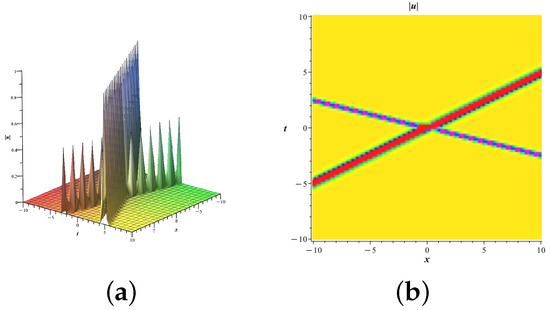
Figure 7. Moduli graphic of the double-soliton solution (a) and its density distribution (b) via (34) with $\delta =2,{\lambda }_1=1+2\mathrm{i},{\lambda }_2=2-\mathrm{i},{\alpha }_1=1,{\alpha }_2=\mathrm{i},{\beta }_1=\mathrm{i},{\beta }_2=1$.

Figure 8. Moduli graphics of the double-soliton solution and its density distribution via (34) with $\delta =2$ and (a,d) ${\lambda }_1=1+0.5\mathrm{i},{\lambda }_2=0.5-\mathrm{i},{\alpha }_1={\displaystyle \frac{\sqrt{2}}{2}}(2+\mathrm{i}),{\alpha }_2=\mathrm{i},{\beta }_1={\displaystyle \frac{\sqrt{2}}{2}}(1-3\mathrm{i})$, ${\beta }_2=1$; (b,e) ${\lambda }_1=1+2\mathrm{i},{\lambda }_2=1-\mathrm{i},{\alpha }_1={\displaystyle \frac{\sqrt{2}}{2}}(4+\mathrm{i}),{\alpha }_2=\mathrm{i},{\beta }_1={\displaystyle \frac{\sqrt{2}}{2}}(1-4\mathrm{i}),{\beta }_2=0.5\mathrm{i}$; (c,f) ${\lambda }_1={\displaystyle \frac{\sqrt{2}}{2}}(1+4\mathrm{i}),{\lambda }_2={\displaystyle \frac{\sqrt{2}}{2}}(1-2\mathrm{i}),{\alpha }_1=\mathrm{i},{\alpha }_2=1,{\beta }_1=0.5\mathrm{i},{\beta }_2=1$.

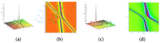
Figure 9. Moduli graphics of the double-soliton solution and its density distribution via (34) with $\delta =2$ and (a,b) ${\lambda }_1=-1+0.5\mathrm{i},{\lambda }_2=0.5-\mathrm{i},{\alpha }_1=1,{\alpha }_2=-\mathrm{i},{\beta }_1=-\mathrm{i},{\beta }_2=1$; (c,d) ${\lambda }_1=-1+0.5\mathrm{i},{\lambda }_2=0.5-\mathrm{i},{\alpha }_1=1,{\alpha }_2=-\mathrm{i},{\beta }_1=0.5\mathrm{i},{\beta }_2=-0.5$.

In the actual optical fiber communication system, the optical pulses may interact with each other, so it is important to study the interaction characteristics of the double-soliton solution. By analyzing the solution of double solitons, we find that the interaction is mainly divided into collision and non-collision cases.

When two solitons do not collide, their directions of motion may be parallel or offset due to interaction. In the case of parallel motion, as shown in Figure 2, the double soliton solution has similar stability to the single soliton solution, and its amplitude does not change with time.

In the other case, when the direction of motion is shifted, the solitons’ stability is still maintained despite the interaction between them (see Figure 3).

When two solitons in a double soliton solution collide, there are three main cases: the cross collision produced by the breath, the energy at the collision increased, and the energy at the collision decreased.

Figure 4 shows that under the cross collision of solitons, the solitons appear as breathers, as shown in Figure 4a,b. With the change in the real part of ${\lambda }_1$, the respiratory characteristics of the breathers disappear, and the respirators transform into periodic waves, as shown in Figure 4c,d.

Due to the nonlinear superposition effect of the two solitons and the interaction of the two solitons, the energy is concentrated in the central collision region, and the energy of the collision point is increased. In Figure 5, the energy of the two solitons in Figure 5a is enhanced only at the collision, and the energy remains unchanged before and after the collision, showing good stability. In Figure 5b, we can observe that one of the periodically collapsed solitons decays its amplitude after the collision, while the other non-singular soliton maintains its amplitude before and after the collision. Both solitons in Figure 5c have amplitude attenuation after collision.

In contrast to the increased energy, the energy will be dispersed at the collision center due to nonlinear effects, which will reduce the energy at the collision point. Similar to the situation in Figure 5a, the energy of the two solitons in Figure 6a only decreases at the collision, and the energy remains unchanged before and after the collision; they also have good stability over a long period of time. One soliton in Figure 6b is unchanged in amplitude, while the other is stabilized after attenuation. The two periodically collapsed solitons in Figure 6c, both experienced attenuation.

In particular, as shown in Figure 7, when the two collider solitons are periodically collapsed solitons, the energy increase or decrease at the collision center is small, and it has good stability, which will also provide meaningful theoretical support for the gCLL Equation (2) and the study of simulating ultra-short and high-intensity pulse transmission in nonlinear optical media.

In scenarios where there is an increase or decrease in energy at the collision point, the nonlinear superposition effect and interactions between solitons lead to a concentration or dispersion of energy within the collision region. By adjusting various parameters, we observe the stability of solitons under different energy variations. These findings offer significant theoretical support for analyzing the stability of multi-pulse transmission in optical fiber communication.

For the research of soliton solution dynamics, it is necessary to consider the influence of rogue waves on soliton stability. After study, Figure 8 and Figure 9 show several representative strange waves in the gCLL Equation (2).

The three rogue waves in Figure 8 are produced when soliton collisions occur. The strange wave in Figure 8a is the most common type, and the energy of the soliton in the collision increases dramatically, several times higher than the original amplitude of the soliton. The solitons in Figure 8b are decaying in central energy. Before the collision, we can observe a surge in energy and then a sharp decline in amplitude. Unlike Figure 8a,b, the solitons in Figure 8c do not experience a spike in energy at the center of the collision. The spike in energy is experienced at some point before the collision occurs, and then returns to normal.

The two rogue waves in Figure 9 are produced when the two solitons do not collide. In Figure 9a, the energy of the two solitons increases significantly when the two solitons are closest to each other under the interaction. Similar to Figure 8c, in Figure 9b, solitons do not experience a sudden increase in energy at the closest point but a sudden, sharp increase at some point and then a return to normal.

Clearly, by adjusting different parameters, numerous phenomena worthy of further study can still be observed. We will continue this discussion in subsequent research endeavors.

Remark 1. 

We observe that by removing the self-gradient term and setting $\delta ={\displaystyle \frac{1}{2}}$, the resulting $\mathit{N}$-soliton solution (31) aligns with the $\mathit{N}$-soliton solution of the CLL Equation (1).

$$\begin{array}{cc}\hfill u=& -2\mathrm{i}\sum _{k=1}^N\sum _{j=1}^N{\alpha }_k{\beta }_j^{*}exp\left[{\theta }_k-{\theta }_j^{*}\right]{\left(M^{-1}\right)}_{kj}\hfill \\ \hfill & +2\mathrm{i}\sum _{k=1}^N\sum _{j=N+1}^{2N}{\alpha }_k{\beta }_{j-N}^{*}exp\left[{\theta }_k-{\theta }_{j-N}^{*}\right]{\left(M^{-1}\right)}_{kj}\hfill \\ \hfill & -2\mathrm{i}\sum _{k=N+1}^{2N}\sum _{j=1}^N{\alpha }_{k-N}{\beta }_j^{*}exp\left[{\theta }_{k-N}-{\theta }_j^{*}\right]{\left(M^{-1}\right)}_{kj}\hfill \\ \hfill & +2\mathrm{i}\sum _{k=N+1}^{2N}\sum _{j=N+1}^{2N}{\alpha }_{k-N}{\beta }_{j-N}^{*}exp\left[{\theta }_{k-N}-{\theta }_{j-N}^{*}\right]{\left(M^{-1}\right)}_{kj},\hfill \end{array}$$

where $M={\left(m_{kj}\right)}_{2N\times 2N}$ is a non-singular matrix with

$$m_{kj}=\left\{\begin{array}{c}{\displaystyle \frac{{\alpha }_k^{*}{\alpha }_{j}exp\left[{\theta }_k^{*}+{\theta }_j\right]+{\beta }_k^{*}{\beta }_{j}exp\left[-{\theta }_k^{*}-{\theta }_j\right]}{{\lambda }_j-{\lambda }_k^{*}},}\hfill \\ 1\le k,j\le N,\hfill \\ {\displaystyle \frac{{\alpha }_k^{*}{\alpha }_{j-N}exp\left[{\theta }_k^{*}+{\theta }_{j-N}\right]-{\beta }_k^{*}{\beta }_{j-N}exp\left[-{\theta }_k^{*}-{\theta }_{j-N}\right]}{-{\lambda }_{j-N}-{\lambda }_k^{*}},}\hfill \\ 1\le k\le N,N+1\le j\le 2N,\hfill \\ {\displaystyle \frac{{\alpha }_{k-N}^{*}{\alpha }_{j}exp\left[{\theta }_{k-N}^{*}+{\theta }_j\right]-{\beta }_{k-N}^{*}{\beta }_{j}exp\left[-{\theta }_{k-N}^{*}-{\theta }_j\right]}{{\lambda }_j+{\lambda }_{k-N}^{*}},}\hfill \\ N+1\le k\le 2N,1\le j\le N,\hfill \\ {\displaystyle \frac{{\alpha }_{k-N}^{*}{\alpha }_{j-N}exp\left[{\theta }_{k-N}^{*}+{\theta }_{j-N}\right]+{\beta }_{k-N}^{*}{\beta }_{j-N}exp\left[-{\theta }_{k-N}^{*}-{\theta }_{j-N}\right]}{-{\lambda }_{j-N}+{\lambda }_{k-N}^{*}},}\hfill \\ N+1\le k,j\le 2N,\hfill \end{array}\right.$$

and ${\displaystyle {\theta }_j=-\mathrm{i}{\lambda }_j^{2}x-\mathrm{i}{\lambda }_j^{4}t}$, ${\lambda }_j\in C_{+}$, $j=1,2,\dots ,N$.

Although the coefficient of the second-order partial derivative term of u with respect to x differs from that of the CLL Equation (1), resulting in a different form for ${\theta }_j$, the characterization of the $\mathit{N}$-soliton solution remains consistent.

Furthermore, setting $\delta ={\displaystyle \frac{1}{2}}$ and removing the self-gradient term, (32) reduces to another $\mathit{N}$-soliton solution for the CLL Equation (1).

$$\begin{array}{c}\hfill u=-2\mathrm{i}\sum _{k=1}^N\sum _{j=1}^N{\alpha }_k{\beta }_j^{*}exp\left[{\theta }_k-{\theta }_j^{*}\right]{\left(M^{-1}\right)}_{kj},\end{array}$$

where ${\displaystyle m_{kj}={\left(m_{kj}\right)}_{N\times N}=\frac{{\alpha }_k^{*}{\alpha }_{j}exp\left[{\theta }_k^{*}+{\theta }_j\right]+{\beta }_k^{*}{\beta }_{j}exp\left[-{\theta }_k^{*}-{\theta }_j\right]}{{\lambda }_j-{\lambda }_k^{*}}}$, $1\le k,j\le N$.

5. Conclusions

In this paper, we study a variant of the Chen–Lee–Liu Equation (2) and obtain its $\mathit{N}$-soliton solution by the Riemann–Hilbert approach. We start by conducting spectral analysis of the Lax pair of the generalized Chen–Lee–Liu Equation (2), and then formulate a Riemann–Hilbert problem on the $\lambda$-plane. By solving specific Riemann–Hilbert problems with vanishing scattering coefficients, corresponding to reflection-less cases, we obtain $\mathit{N}$-soliton solutions for (2). The main procedure involves utilizing the symmetry relations of the potential matrix Q. Using these symmetry relations enables us to analyze the zeros of $det{P}_{+}$ and $det{P}_{-}$. It is noteworthy that the well-known Chen–Lee–Liu equation, an important model in fiber optics, is a special case of our proposed generalization. Consequently, $\mathit{N}$-soliton solutions for the Chen–Lee–Liu Equation (1) can be derived by reducing those for (2). Furthermore, by adjusting parameters and conducting comparative analyses, we generate three-dimensional soliton images that warrant further exploration. The stability of soliton solutions is essential for maintaining communication signal integrity, offering new insights into light pulse propagation behavior within optical fibers.

Finally, it is worth noting that a thorough investigation of the long-term asymptotic behavior of soliton solutions can be attempted via the Riemann–Hilbert approach to examine the asymptotic stability of the solutions [42], particularly when the generalized Chen–Lee–Liu Equation (2) is irregular. However, there are various other efficient techniques available for obtaining accurate solutions for nonlinear evolution equations, such as the Darboux transformation [43], the dressing method [44], the bilinear method [45], and so on. The consideration of whether these methods apply to the generalized Chen–Lee–Liu Equation (2) will be reserved for later discussion.

References

- Chen, H.; Lee, Y.; Liu, C. Integrability of nonlinear Hamiltonian systems by inverse scattering method. Phys. Scr. 1979, 20, 490. [Google Scholar] [CrossRef]
- Fan, E. Integrable systems of derivative nonlinear Schrödinger type and their multi-Hamiltonian structure. J. Phys. A Math. Gen. 2001, 34, 513. [Google Scholar] [CrossRef]
- Triki, H.; Babatin, M.; Biswas, A. Chirped bright solitons for Chen–Lee–Liu equation in optical fibers and PCF. Optik 2017, 149, 300–303. [Google Scholar] [CrossRef]
- Newell, A.C. The general structure of integrable evolution equations. Proc. R. Soc. Lond. A Math. Phys. Sci. 1979, 365, 283–311. [Google Scholar]
- Kawata, T.; Kobayashi, N.; Inoue, H. Soliton solutions of the derivative nonlinear Schrödinger equation. J. Phys. Soc. Jpn. 1979, 46, 1008–1015. [Google Scholar] [CrossRef]
- Fan, E. Darboux transformation and soliton-like solutions for the Gerdjikov-Ivanov equation. J. Phys. A Math. Gen. 2000, 33, 6925. [Google Scholar] [CrossRef]
- Xu, M.J.; Xia, T.C.; Hu, B.B. Riemann–Hilbert approach and N-soliton solutions for the Chen–Lee–Liu equation. Mod. Phys. Lett. B 2019, 33, 1950002. [Google Scholar] [CrossRef]
- Han, S.H.; Park, Q.H. Effect of self-steepening on optical solitons in a continuous wave background. Phys. Rev. E—Stat. Nonlinear Soft Matter Phys. 2011, 83, 066601. [Google Scholar] [CrossRef]
- Paliathanasis, A. Periodic solutions from Lie symmetries for the generalized Chen–Lee–Liu equation. Eur. Phys. J. Plus 2021, 136, 934. [Google Scholar] [CrossRef]
- Rogers, C.; Chow, K. Localized pulses for the quintic derivative nonlinear Schrödinger equation on a continuous-wave background. Phys. Rev. E Stat. Nonlinear Soft Matter Phys. 2012, 86, 037601. [Google Scholar] [CrossRef]
- Ivanov, S.K. Riemann problem for the light pulses in optical fibers for the generalized Chen-Lee-Liu equation. Phys. Rev. A 2020, 101, 053827. [Google Scholar] [CrossRef]
- Forest, M.; Rosenberg, C.J.; Wright, O. On the exact solution for smooth pulses of the defocusing nonlinear Schrödinger modulation equations prior to breaking. Nonlinearity 2009, 22, 2287. [Google Scholar] [CrossRef]
- González-Gaxiola, O.; Biswas, A. W-shaped optical solitons of Chen–Lee–Liu equation by Laplace–Adomian decomposition method. Opt. Quantum Electron. 2018, 50, 314. [Google Scholar] [CrossRef]
- Liu, N.; Sun, J.; Yu, J.D. Inverse scattering and soliton dynamics for the mixed Chen–Lee–Liu derivative nonlinear Schrödinger equation. Appl. Math. Lett. 2024, 152, 109029. [Google Scholar] [CrossRef]
- Zhang, N.; Xia, T.c.; Fan, E.g. A Riemann-Hilbert approach to the Chen-Lee-Liu equation on the half line. Acta Math. Appl. Sin. Engl. Ser. 2018, 34, 493–515. [Google Scholar] [CrossRef]
- Ozdemir, N.; Esen, H.; Secer, A.; Bayram, M.; Yusuf, A.; Sulaiman, T.A. Optical soliton solutions to Chen Lee Liu model by the modified extended tanh expansion scheme. Optik 2021, 245, 167643. [Google Scholar] [CrossRef]
- Yıldırım, Y. Optical solitons to Chen–Lee–Liu model in birefringent fibers with trial equation approach. Optik 2019, 183, 881–886. [Google Scholar] [CrossRef]
- Bansal, A.; Biswas, A.; Zhou, Q.; Arshed, S.; Alzahrani, A.K.; Belic, M.R. Optical solitons with Chen–Lee–Liu equation by Lie symmetry. Phys. Lett. A 2020, 384, 126202. [Google Scholar] [CrossRef]
- Gomez, C.A.; Rezazadeh, H.; Inc, M.; Akinyemi, L.; Nazari, F. The generalized Chen-Lee-Liu model with higher order nonlinearity: Optical solitons. Opt. Quantum Electron. 2022, 54, 492. [Google Scholar] [CrossRef]
- Scott, A.C.; Chu, F.Y.; McLaughlin, D.W. The soliton: A new concept in applied science. Proc. IEEE 1973, 61, 1443–1483. [Google Scholar] [CrossRef]
- Hirota, R. The Direct Method in Soliton Theory; Cambridge University Press: Cambridge, UK, 2004; p. 155. [Google Scholar]
- Gu, C. Soliton Theory and Its Applications; Springer Science & Business Media: Berlin/Heidelberg, Germany, 2013. [Google Scholar]
- Ablowitz, M.J.; Segur, H. Solitons and the Inverse Scattering Transform; SIAM: Bangkok, Thailand, 1981. [Google Scholar]
- Wazwaz, A.M. Multiple-soliton solutions for the KP equation by Hirota’s bilinear method and by the tanh–coth method. Appl. Math. Comput. 2007, 190, 633–640. [Google Scholar] [CrossRef]
- Gu, C.; Hu, H.; Zhou, Z. Darboux Transformations in Integrable Systems: Theory and Their Applications to Geometry; Springer Science & Business Media: Berlin/Heidelberg, Germany, 2004. [Google Scholar]
- Rogers, C.; Schief, W.K. Bäcklund and Darboux Transformations: Geometry and Modern Applications in Soliton Theory; Cambridge University Press: Cambridge, UK, 2002; Volume 30. [Google Scholar]
- Aygar, Y.; Bairamov, E. Jost solution and the spectral properties of the matrix-valued difference operators. Appl. Math. Comput. 2012, 218, 9676–9681. [Google Scholar] [CrossRef]
- Miller, R.K. Volterra integral equations in a Banach space. Funkcial. Ekvac 1975, 18, 163–193. [Google Scholar]
- Zhang, Y.; Cheng, Y.; He, J. Riemann—Hilbert method and N—soliton for two—component Gerdjikov-Ivanov equation. J. Nonlinear Math. Phys. 2017, 24, 210–223. [Google Scholar] [CrossRef]
- Lenells, J.; Fokas, A. An integrable generalization of the nonlinear Schrödinger equation on the half-line and solitons. Inverse Probl. 2009, 25, 115006. [Google Scholar] [CrossRef]
- Guo, B.; Ling, L. Riemann-Hilbert approach and N-soliton formula for coupled derivative Schrödinger equation. J. Math. Phys. 2012, 53, 073506. [Google Scholar] [CrossRef]
- Fokas, A.S. Two–dimensional linear partial differential equations in a convex polygon. Proc. R. Soc. Lond. Ser. A Math. Phys. Eng. Sci. 2001, 457, 371–393. [Google Scholar] [CrossRef]
- Shchesnovich, V.S.; Yang, J. General soliton matrices in the Riemann–Hilbert problem for integrable nonlinear equations. J. Math. Phys. 2003, 44, 4604–4639. [Google Scholar] [CrossRef]
- Faddeev, L.D.; Takhtajan, L.A. Hamiltonian Methods in the Theory of Solitons; Springer: Berlin/Heidelberg, Germany, 1987; Volume 23. [Google Scholar]
- Wang, D.S.; Ma, Y.Q.; Li, X.G. Prolongation structures and matter-wave solitons in F = 1 spinor Bose–Einstein condensate with time-dependent atomic scattering lengths in an expulsive harmonic potential. Commun. Nonlinear Sci. Numer. Simul. 2014, 19, 3556–3569. [Google Scholar] [CrossRef]
- Geng, X.; Wu, J. Riemann–Hilbert approach and N-soliton solutions for a generalized Sasa–Satsuma equation. Wave Motion 2016, 60, 62–72. [Google Scholar] [CrossRef]
- Boutet de Monvel, A.; Shepelsky, D.; Zielinski, L. The short pulse equation by a Riemann–Hilbert approach. Lett. Math. Phys. 2017, 107, 1345–1373. [Google Scholar] [CrossRef]
- Kang, Z.Z.; Xia, T.C.; Ma, X. Multi-soliton solutions for the coupled modified nonlinear Schrödinger equations via Riemann–Hilbert approach. Chin. Phys. B 2018, 27, 070201. [Google Scholar] [CrossRef]
- Ma, W.X. Riemann–Hilbert problems and N-soliton solutions for a coupled mKdV system. J. Geom. Phys. 2018, 132, 45–54. [Google Scholar] [CrossRef]
- Zhuang, Y.; Zhang, Y.; Zhang, H.; Xia, P. Multi-soliton solutions for the three types of nonlocal Hirota equations via Riemann–Hilbert approach. Commun. Theor. Phys. 2022, 74, 115004. [Google Scholar] [CrossRef]
- Lin, Y.; Dong, H.; Fang, Y. N-Soliton Solutions for the NLS-Like Equation and Perturbation Theory Based on the Riemann–Hilbert Problem. Symmetry 2019, 11, 826. [Google Scholar] [CrossRef]
- Qiu, D. Riemann-Hilbert approach and N-soliton solution for the Chen-Lee-Liu equation. Eur. Phys. J. Plus 2021, 136, 825. [Google Scholar] [CrossRef]
- Matveev, V.B.; Salle, M.A. Darboux Transformations and Solitons; Springer Series in Nonlinear Dynamics; Springer: Berlin/Heidelberg, Germany, 1991. [Google Scholar]
- Lenells, J. Dressing for a novel integrable generalization of the nonlinear Schrödinger equation. J. Nonlinear Sci. 2010, 20, 709–722. [Google Scholar] [CrossRef]
- Liu, W.J.; Tian, B.; Zhang, H.Q.; Li, L.L.; Xue, Y.S. Soliton interaction in the higher-order nonlinear Schrödinger equation investigated with Hirota’s bilinear method. Phys. Rev. E—Stat. Nonlinear Soft Matter Phys. 2008, 77, 066605. [Google Scholar] [CrossRef]
Disclaimer/Publisher’s Note: The statements, opinions and data contained in all publications are solely those of the individual author(s) and contributor(s) and not of MDPI and/or the editor(s). MDPI and/or the editor(s) disclaim responsibility for any injury to people or property resulting from any ideas, methods, instructions or products referred to in the content. |
© 2025 by the authors. Licensee MDPI, Basel, Switzerland. This article is an open access article distributed under the terms and conditions of the Creative Commons Attribution (CC BY) license (https://creativecommons.org/licenses/by/4.0/).