Fractional Operator Approach and Hybrid Special Polynomials: The Generalized Gould–Hopper–Bell-Based Appell Polynomials and Their Characteristics

Abstract

This study introduces a novel generalized class of special polynomials using a fractional operator approach. These polynomials are referred to as the generalized Gould–Hopper–Bell-based Appell polynomials. In view of the operational method, we first introduce the operational representation of the Gould–Hopper–Bell-based Appell polynomials; then, using a fractional operator, we establish a new generalized form of these polynomials. The associated generating function, series representations, and summation formulas are also obtained. Additionally, certain operational identities, as well as determinant representation, are derived. The investigation further explores specific members of this generalized family, including the generalized Gould–Hopper–Bell-based Bernoulli polynomials, the generalized Gould–Hopper–Bell-based Euler polynomials, and the generalized Gould–Hopper–Bell-based Genocchi polynomials, revealing analogous results for each. Finally, the study employs Mathematica to present computational outcomes, zero distributions, and graphical representations associated with the special member, generalized Gould–Hopper–Bell-based Bernoulli polynomials.

1. Introduction

Special functions, rooted in centuries of development and supported by an extensive body of literature, are characterized by their nuanced definitions and broad applicability—both within mathematics and beyond its boundaries. These functions have long played a pivotal role in advancing pure and applied mathematics, engineering, physics, and other disciplines that rely on mathematical methodologies as fundamental tools.

The investigation of special polynomials and numbers has long served as a prominent domain within mathematical analysis, intersecting with diverse disciplines, such as differential and integral equations, fractional calculus, and mathematical physics, over many decades. Moreover, these special polynomials enable the effortless generation of a wide range of useful identities and are instrumental in defining new categories of special polynomials. Among the most significant are the Appell polynomials, the Gould–Hopper polynomials, and the Bell polynomials, which are highly valued for their wide-ranging applications in various mathematical contexts.

The Gould–Hopper polynomials (GHP), denoted as ${\mathcal{H}}_{\delta }^{\left(r\right)}({\nu }_1,{\nu }_2)$ [1], are characterized by

$$exp\left({\nu }_1\omega +{\nu }_2{\omega }^r\right)=\sum _{\delta =0}^{\infty }{\mathcal{H}}_{\delta }^{\left(r\right)}({\nu }_1,{\nu }_2){\displaystyle \frac{{\omega }^{\delta }}{\delta !}}.$$

For $r=2$, the GHP ${\mathcal{H}}_{\delta }^{\left(r\right)}({\nu }_1,{\nu }_2)$ reduce to the two-variable Hermite Kampé de Fériet polynomials (2VHKDFP) ${\mathcal{H}}_{\delta }^{\left(2\right)}({\nu }_1,{\nu }_2)$ [2], which are characterized by

$$exp\left({\nu }_1\omega +{\nu }_2{\omega }^2\right)=\sum _{\delta =0}^{\infty }{\mathcal{H}}_{\delta }^{\left(2\right)}({\nu }_1,{\nu }_2){\displaystyle \frac{{\omega }^{\delta }}{\delta !}}.$$

The two-variable Bell polynomials (2VBelP), denoted as $\mathcal{B}e{l}_{\delta }({\nu }_1,{\nu }_2)$ [3], are characterized by

$$exp({\nu }_1\omega +{\nu }_2(e^{\omega }-1))=\sum _{\delta =0}^{\infty }\mathcal{B}e{l}_{\delta }({\nu }_1,{\nu }_2){\displaystyle \frac{{\omega }^{\delta }}{\delta !}}.$$

(1)

Taking ${\nu }_1=0$ in generating function (1), we obtain

$$exp\left({\nu }_2(e^{\omega }-1)\right)=\sum _{\delta =0}^{\infty }\mathcal{B}e{l}_{\delta }\left({\nu }_2\right){\displaystyle \frac{{\omega }^{\delta }}{\delta !}},$$

(2)

where $\mathcal{B}e{l}_{\delta }\left({\nu }_2\right)$ denotes the classical Bell polynomials [4].

The Appell polynomials, as discussed in [5], represent a prominent and significant category of specialized polynomial sequences. Research on these polynomials has remained a vibrant area of investigation, due to their broad utility in diverse fields, including approximation theory, theoretical physics, analytic number theory, and numerous other branches of mathematics. An application of the Appell polynomials in probability theory and statistics is exemplified in [6,7]. The generalized Appell polynomials were first presented in [8] as tools to approximate three-dimensional mappings alongside methodologies derived from Clifford analysis. Findings in representation theory, such as those in [9,10], demonstrate new applications of the Appell polynomials and emphasize their essential function as orthogonal polynomials. Additionally, representation theory serves as a foundational tool for their use in quantum physics, as elaborated in [11]. The Appell polynomials are specified through their generating functions:

$$\mathcal{A}\left(\omega \right)exp\left({\nu }_1\omega \right)=\sum _{\delta =0}^{\infty }{\mathcal{A}}_{\delta }\left({\nu }_1\right){\displaystyle \frac{{\omega }^{\delta }}{\delta !}},$$

where

$$\mathcal{A}\left(\omega \right)=\sum _{\delta =0}^{\infty }{\mathcal{A}}_{\delta }{\displaystyle \frac{{\omega }^{\delta }}{\delta !}},{\mathcal{A}}_0\ne 0$$

(3)

which is an analytic function at $\omega =0$, and ${\mathcal{A}}_{\delta }:={\mathcal{A}}_{\delta }\left(0\right)$ denotes the Appell numbers. By inspection, it is clear that for any $\mathcal{A}\left(\omega \right)$, the derivative of $\mathcal{A}\left(\omega \right)$ satisfies

$${\displaystyle \frac{d}{d{\nu }_1}}{\mathcal{A}}_{\delta }\left({\nu }_1\right)=\delta {\mathcal{A}}_{\delta -1}\left({\nu }_1\right).$$

The class of Appell sequences encompasses numerous classical polynomial sequences, including the Bernoulli, Euler, and Genocchi polynomials. Recent research has introduced and explored novel categories of hybrid special polynomials related to the Appell polynomials [12,13,14,15,16,17,18,19,20,21,22]. These hybrid polynomials hold significant interest, due to their possession of critical mathematical properties, such as series and determinant definitions, generating functions, differential equations, and other foundational characteristics.

Recently, Muhyi [23] introduced the Gould–Hopper–Bell–Appell polynomials (GHBelAP) ${}_{\mathcal{H}\mathcal{B}el}\mathcal{A}_{\delta }^{\left(r\right)}({\nu }_1,{\nu }_2,z)$, which are characterized by

$$\mathcal{A}\left(\omega \right)exp\left({\nu }_1\omega +{\nu }_2{\omega }^r+z(e^{\omega }-1)\right)=\sum _{\delta =0}^{\infty }{}_{\mathcal{H}\mathcal{B}el}\mathcal{A}_{\delta }^{\left(r\right)}({\nu }_1,{\nu }_2,z){\displaystyle \frac{{\omega }^{\delta }}{\delta !}}.$$

(4)

The series definition of the GHBelAP ${}_{\mathcal{H}\mathcal{B}el}\mathcal{A}_{\delta }^{\left(r\right)}({\nu }_1,{\nu }_2,z)$ is given as

$${}_{\mathcal{H}\mathcal{B}el}\mathcal{A}_{\delta }^{\left(r\right)}({\nu }_1,{\nu }_2,z)=\delta !\sum _{\kappa =0}^{\left[{\displaystyle \frac{\delta }{r}}\right]}{\displaystyle \frac{{\nu }_2^{\kappa }{}_{\mathcal{B}el}\mathcal{A}_{\delta -rk}({\nu }_1,z)}{\kappa !(\delta -r\kappa )!}}.$$

(5)

Taking ${\nu }_2=0$ in (4), the GHBelAP ${}_{\mathcal{H}\mathcal{B}el}\mathcal{A}_{\delta }^{\left(r\right)}({\nu }_1,{\nu }_2,z)$ reduce to the two-variable Bell–Appell polynomials (BelAP) ${}_{\mathcal{B}el}\mathcal{A}_{\delta }({\nu }_1,z)$ [24], which are defined by

$$\mathcal{A}\left(\omega \right)exp\left({\nu }_1\omega +z(e^{\omega }-1)\right)=\sum _{\delta =0}^{\infty }{}_{\mathcal{B}el}\mathcal{A}_{\delta }({\nu }_1,z){\displaystyle \frac{{\omega }^{\delta }}{\delta !}}.$$

(6)

Taking $z=0$ in (4), the GHBelAP ${}_{\mathcal{H}\mathcal{B}el}\mathcal{A}_{\delta }^{\left(r\right)}({\nu }_1,{\nu }_2,z)$ reduce to the Gould–Hopper–Appell polynomials ${}_{\mathcal{H}}\mathcal{A}_{\delta }^{\left(r\right)}({\nu }_1,{\nu }_2)$ [25], which are defined by

$$\mathcal{A}\left(\omega \right)exp\left({\nu }_1\omega +{\nu }_2{\omega }^r\right)=\sum _{\delta =0}^{\infty }{}_{\mathcal{H}}\mathcal{A}_{\delta }^{\left(r\right)}({\nu }_1,{\nu }_2){\displaystyle \frac{{\omega }^{\delta }}{\delta !}}.$$

Taking $\mathcal{A}\left(\omega \right)=1$ in (4), the GHBelAP ${}_{\mathcal{H}\mathcal{B}el}\mathcal{A}_{\delta }^{\left(r\right)}({\nu }_1,{\nu }_2,z)$ reduce to the Gould–Hopper–Bell polynomials ${}_{\mathcal{H}}\mathcal{B}e{l}_{\delta }^{\left(r\right)}({\nu }_1,{\nu }_2)$ [26], which are defined by

$$exp\left({\nu }_1\omega +{\nu }_2{\omega }^r+z(e^{\omega }-1)\right)=\sum _{\delta =0}^{\infty }{}_{\mathcal{H}}\mathcal{B}e{l}_{\delta }^{\left(r\right)}({\nu }_1,{\nu }_2,z){\displaystyle \frac{{\omega }^{\delta }}{\delta !}}.$$

Moreover, depending on the selection of the function $\mathcal{A}\left(\omega \right)$, the GHBelAP ${}_{\mathcal{H}\mathcal{B}el}\mathcal{A}_{\delta }^{\left(r\right)}({\nu }_1,{\nu }_2,z)$ simplify to specific special polynomials, which are outlined as special cases in

Table 1. Certain members of the GHBelAP ${}_{\mathcal{H}\mathcal{B}el}\mathcal{A}_{\delta }^{\left(r\right)}({\nu }_1,{\nu }_2,z)$.

S.No.	$\mathcal{A}\left(\mathit{\omega }\right)$	Polynomials	Generating Function
I.	${\displaystyle \frac{\omega }{e^{\omega }-1}}$	Gould–Hopper–Bell–Bernoulli	${\displaystyle \frac{\omega }{e^{\omega }-1}}exp\left({\nu }_1\omega +{\nu }_2{\omega }^r+z(e^{\omega }-1)\right)$
		polynomials	$={\sum }_{\delta =0}^{\infty }{}_{\mathcal{H}\mathcal{B}el}\mathcal{B}_{\delta }^{\left(r\right)}({\nu }_1,{\nu }_2,z){\displaystyle \frac{{\omega }^{\delta }}{\delta !}}$
II.	${\displaystyle \frac{2}{e^{\omega }+1}}$	Gould–Hopper–Bell–Euler	${\displaystyle \frac{2}{e^{\omega }+1}}exp\left({\nu }_1\omega +{\nu }_2{\omega }^r+z(e^{\omega }-1)\right)$
		polynomials	$={\sum }_{\delta =0}^{\infty }{}_{\mathcal{H}\mathcal{B}el}\mathcal{E}_{\delta }^{\left(r\right)}({\nu }_1,{\nu }_2,z){\displaystyle \frac{{\omega }^{\delta }}{\delta !}}$
III.	${\displaystyle \frac{2\omega }{e^{\omega }+1}}$	Gould–Hopper–Bell–Genocchi	${\displaystyle \frac{2\omega }{e^{\omega }+1}}exp\left({\nu }_1\omega +{\nu }_2{\omega }^r+z(e^{\omega }-1)\right)$
		polynomials	$={\sum }_{\delta =0}^{\infty }{}_{\mathcal{H}\mathcal{B}el}\mathcal{G}_{\delta }^{\left(r\right)}({\nu }_1,{\nu }_2,z){\displaystyle \frac{{\omega }^{\delta }}{\delta !}}$

[23]:

Over the last four decades, the combination of fractional calculus and integral transforms has grown into a vital cross-disciplinary field, driven predominantly by its widespread utility across diverse science and engineering domains. In addition, fractional calculus serves as a powerful framework for uncovering novel properties and relationships within special polynomials. By leveraging fractional operators on well-known special polynomials, new generalizations of hybrid forms of special polynomials can be introduced [27,28,29,30,31,32].

Here, we recall one of the useful fractional operators in special polynomials, the Euler integral, which was presented by Srivastava and Manocha [33]. By leveraging the Euler integral as a foundational tool, researchers successfully uncovered novel pathways for advancing the study of special polynomial theory. Dattoli et al. [28,29] have made substantial contributions to the theory and application of special polynomials, particularly through their exploitation of the Euler integral representation. The Euler integral ([33], p. 218) is defined as

$${\eta }^{-\sigma }={\displaystyle \frac{1}{\Gamma \left(\sigma \right)}}{\mathit{\int }}_0^{\infty }{e}^{-\eta \xi }{\xi }^{\sigma -1}d\xi ,min\left\{\Re \left(\eta \right),\Re \left(\sigma \right)\right\}>0,$$

(7)

which leads to the following [29]:

$${\left[\eta -{\displaystyle \frac{\partial }{\partial \nu }}\right]}^{-\sigma }f\left(\nu \right)={\displaystyle \frac{1}{\Gamma \left(\sigma \right)}}{\mathit{\int }}_0^{\infty }{e}^{-\eta \xi }{\xi }^{\sigma -1}exp\left(\xi {\displaystyle \frac{\partial }{\partial \nu }}\right)f\left(\nu \right)d\xi$$

and, consequently, we can obtain

$${\left[\eta -{\displaystyle \frac{{\partial }^r}{\partial {\nu }^r}}\right]}^{-\sigma }f\left(\nu \right)={\displaystyle \frac{1}{\Gamma \left(\sigma \right)}}{\mathit{\int }}_0^{\infty }{e}^{-\eta \xi }{\xi }^{\sigma -1}exp\left(\xi {\displaystyle \frac{{\partial }^r}{\partial {\nu }^r}}\right)f\left(\nu \right)d\xi .$$

An efficient application of fractional operators can be achieved through the combination of exponential operator properties and well-chosen integral representations.

The novelty of this study lies in establishing a generalized family of special polynomials. This study advances the application of fractional operational methods to construct a versatile class of polynomials that generalizes and extends existing families (e.g., the Gould–Hopper, Bell, Appell, Gould–Hopper–Bell, Bernoulli, Euler, Genocchi, Gould–Hopper–Bernoulli, Gould–Hopper–Euler, Gould–Hopper–Genocchi, Bell–Bernoulli, Bell–Euler, and Bell–Genocchi polynomials [1,3,23,24,25,26,34,35,36]), which expands the theory of special function by introducing and systematically studying a new, broad class of polynomials. This framework demonstrates the utility and flexibility of fractional operational methods in constructing and analyzing generalized polynomial structures. Furthermore, connecting special polynomials to fractional calculus points towards potential uses in areas where fractional derivatives are important.

The motivation for this work stems from the contributions of Dattoli [28], Dattoli et al. [29], Khan et al. [30,32], and Yasmin and Muhyi [31], who highlighted the importance of fractional operators in advancing theoretical and applied frameworks in the area of special functions. In this study, we introduce a generalized family of special polynomials constructed through a fractional operator framework, designated as the generalized Gould–Hopper–Bell–Appell polynomials. In Section 2, we first employ operational techniques to establish the operational formulation of the Gould–Hopper–Bell–Appell polynomials. Subsequently, we extend this framework by incorporating fractional operators, to develop a broader generalization of these polynomials. Corresponding generating functions, series expressions, and summation relations are also derived. Section 3 focuses on deriving operational properties and determinant-based representations. Section 4 investigates specific cases within this generalized family, such as the generalized Gould–Hopper–Bell-based Bernoulli polynomials, the generalized Gould–Hopper–Bell-based Euler polynomials, and the generalized Gould-Hopper-Bell-based Genocchi polynomials, revealing analogous results for each. In Section 5, computational outcomes, zero distributions, and graphical visualizations for the generalized Gould–Hopper–Bell–Bernoulli polynomials are generated, using Mathematica. These results provide numerical and visual insights into the behavior of these polynomials.

2. The Generalized Gould–Hopper–Bell–Appell Polynomials

In this section, we first derive an operational relation between the GHBelAP ${}_{\mathcal{H}\mathcal{B}el}\mathcal{A}_{\delta }^{\left(r\right)}({\nu }_1,{\nu }_2,z)$ and the BelAP ${}_{\mathcal{B}el}\mathcal{A}_{\delta }({\nu }_1,{\nu }_2)$. Then, based on the obtained operational representation and in view of the Euler integral, we establish the generalized Gould–Hopper–Bell–Appell polynomials.

On differentiating the left-hand side of expression (4), with respect to ${\nu }_1$, we find

$${\displaystyle \frac{\partial }{\partial {\nu }_1}}\left[\mathcal{A}\left(\omega \right)exp\left({\nu }_1\omega +{\nu }_2{\omega }^r+z(e^{\omega }-1)\right)\right]=\omega \left[\mathcal{A}\left(\omega \right)exp\left({\nu }_1\omega +{\nu }_2{\omega }^r+z(e^{\omega }-1)\right)\right],$$

which gives

$${\displaystyle \frac{\partial }{\partial {\nu }_1}}\left[\sum _{\delta =0}^{\infty }{}_{\mathcal{H}\mathcal{B}el}\mathcal{A}_{\delta }^{\left(r\right)}({\nu }_1,{\nu }_2,z){\displaystyle \frac{{\omega }^{\delta }}{\delta !}}\right]=\omega \left[\sum _{\delta =0}^{\infty }{}_{\mathcal{H}\mathcal{B}el}\mathcal{A}_{\delta }^{\left(r\right)}({\nu }_1,{\nu }_2,z){\displaystyle \frac{{\omega }^{\delta }}{\delta !}}\right],$$

which, on equating coefficients of like powers of $\omega$, leads to

$${\displaystyle \frac{\partial }{\partial {\nu }_1}}\left[{}_{\mathcal{H}\mathcal{B}el}\mathcal{A}_{\delta }^{\left(r\right)}({\nu }_1,{\nu }_2,z)\right]=\delta \left[{}_{\mathcal{H}\mathcal{B}el}\mathcal{A}_{\delta -1}^{\left(r\right)}({\nu }_1,{\nu }_2,z)\right].$$

Similarly, we can obtain

$$\begin{array}{cc}\hfill & {\displaystyle \frac{{\partial }^2}{\partial {\nu }_1^2}}\left[{}_{\mathcal{H}\mathcal{B}el}\mathcal{A}_{\delta }^{\left(r\right)}({\nu }_1,{\nu }_2,z)\right]=\delta (\delta -1)\left[{}_{\mathcal{H}\mathcal{B}el}\mathcal{A}_{\delta -2}^{\left(r\right)}({\nu }_1,{\nu }_2,z)\right],\hfill \\ & {\displaystyle \frac{{\partial }^3}{\partial {\nu }_1^3}}\left[{}_{\mathcal{H}\mathcal{B}el}\mathcal{A}_{\delta }^{\left(r\right)}({\nu }_1,{\nu }_2,z)\right]=\delta (\delta -1)(\delta -2)\left[{}_{\mathcal{H}\mathcal{B}el}\mathcal{A}_{\delta -3}^{\left(r\right)}({\nu }_1,{\nu }_2,z)\right],\hfill \\ & ⋮\hfill \\ \hfill & \hfill {\displaystyle \frac{{\partial }^r}{\partial {\nu }_1^r}}\left[{}_{\mathcal{H}\mathcal{B}el}\mathcal{A}_{\delta }^{\left(r\right)}({\nu }_1,{\nu }_2,z)\right]=\delta (\delta -1)(\delta -2)\dots (\delta -r+1)\left[{}_{\mathcal{H}\mathcal{B}el}\mathcal{A}_{\delta -r}^{\left(r\right)}({\nu }_1,{\nu }_2,z)\right].\end{array}$$

(8)

Next, on differentiating the left-hand side of expression (4), with respect to ${\nu }_2$, we find

$${\displaystyle \frac{\partial }{\partial {\nu }_2}}\left[\mathcal{A}\left(\omega \right)exp\left({\nu }_1\omega +{\nu }_2{\omega }^r+z(e^{\omega }-1)\right)\right]={\omega }^r\left[\mathcal{A}\left(\omega \right)exp\left({\nu }_1\omega +{\nu }_2{\omega }^r+z(e^{\omega }-1)\right)\right],$$

which gives

$${\displaystyle \frac{\partial }{\partial {\nu }_2}}\left[\sum _{\delta =0}^{\infty }{}_{\mathcal{H}\mathcal{B}el}\mathcal{A}_{\delta }^{\left(r\right)}({\nu }_1,{\nu }_2,z){\displaystyle \frac{{\omega }^{\delta }}{\delta !}}\right]={\omega }^r\left[\sum _{\delta =0}^{\infty }{}_{\mathcal{H}\mathcal{B}el}\mathcal{A}_{\delta }^{\left(r\right)}({\nu }_1,{\nu }_2,z){\displaystyle \frac{{\omega }^{\delta }}{\delta !}}\right],$$

which, on equating coefficients of like powers of $\omega$, leads to

$${\displaystyle \frac{\partial }{\partial {\nu }_2}}\left[{}_{\mathcal{H}\mathcal{B}el}\mathcal{A}_{\delta }^{\left(r\right)}({\nu }_1,{\nu }_2,z)\right]=\delta (\delta -1)(\delta -2)\dots (\delta -r+1)\left[{}_{\mathcal{H}\mathcal{B}el}\mathcal{A}_{\delta -r}^{\left(r\right)}({\nu }_1,{\nu }_2,z)\right].$$

(9)

From Equations (8) and (9), we obtain

$${\displaystyle \frac{{\partial }^r}{\partial {\nu }_1^r}}\left[{}_{\mathcal{H}\mathcal{B}el}\mathcal{A}_{\delta }^{\left(r\right)}({\nu }_1,{\nu }_2,z)\right]={\displaystyle \frac{\partial }{\partial {\nu }_2}}\left[{}_{\mathcal{H}\mathcal{B}el}\mathcal{A}_{\delta }^{\left(r\right)}({\nu }_1,{\nu }_2,z)\right]$$

(10)

and from Equations (4) and (6), it follows that

$${}_{\mathcal{H}\mathcal{B}el}\mathcal{A}_{\delta }^{\left(r\right)}({\nu }_1,0,z)={}_{\mathcal{B}el}\mathcal{A}_{\delta }({\nu }_1,z).$$

(11)

Solving Equation (10), subject to initial condition (11), we obtain

$${}_{\mathcal{H}\mathcal{B}el}\mathcal{A}_{\delta }^{\left(r\right)}({\nu }_1,{\nu }_2,z)=exp\left({\nu }_2{\displaystyle \frac{{\partial }^r}{\partial {\nu }_1^r}}\right){}_{\mathcal{B}el}\mathcal{A}_{\delta }({\nu }_1,z).$$

(12)

Now, we establish the generalized Gould–Hopper–Bell–Appell polynomials by proving the following results:

Theorem 1.

The generalized Gould–Hopper–Bell–Appell polynomials ${}_{\mathcal{H}\mathcal{B}el}\mathcal{A}_{\delta ,\sigma }^{\left(r\right)}({\nu }_1,{\nu }_2,z;\eta )$ are defined by

$${\left[\eta -{\nu }_2{\displaystyle \frac{{\partial }^r}{\partial {\nu }_1^r}}\right]}^{-\sigma }{}_{\mathcal{B}el}\mathcal{A}_{\delta }({\nu }_1,z)={}_{\mathcal{H}\mathcal{B}el}\mathcal{A}_{\delta ,\sigma }^{\left(r\right)}({\nu }_1,{\nu }_2,z;\eta ).$$

(13)

Proof. 

Replacing $\eta$ by $\left[\eta -{\nu }_2{\displaystyle \frac{{\partial }^r}{\partial {\nu }_1^r}}\right]$ in relation to (7), then applying the resultant relation to ${}_{\mathcal{B}el}\mathcal{A}_{\delta }({\nu }_1,z)$, we obtain the following transformation:

$${\left[\eta -{\nu }_2{\displaystyle \frac{{\partial }^r}{\partial {\nu }_1^r}}\right]}^{-\sigma }{}_{\mathcal{B}el}\mathcal{A}_{\delta }({\nu }_1,z)={\displaystyle \frac{1}{\Gamma \left(\sigma \right)}}{\mathit{\int }}_0^{\infty }{e}^{-\eta \xi }{\xi }^{\sigma -1}exp\left(\xi {\nu }_2{\displaystyle \frac{{\partial }^r}{\partial {\nu }_1^r}}\right){}_{\mathcal{B}el}\mathcal{A}_{\delta }({\nu }_1,z)d\xi ,$$

which, on using operational relation (12), becomes

$${\left[\eta -{\nu }_2{\displaystyle \frac{{\partial }^r}{\partial {\nu }_1^r}}\right]}^{-\sigma }{}_{\mathcal{B}el}\mathcal{A}_{\delta }({\nu }_1,z)={\displaystyle \frac{1}{\Gamma \left(\sigma \right)}}{\mathit{\int }}_0^{\infty }{e}^{-\eta \xi }{\xi }^{\sigma -1}{}_{\mathcal{H}\mathcal{B}el}\mathcal{A}_{\delta }^{\left(r\right)}({\nu }_1,\xi {\nu }_2,z)d\xi .$$

(14)

We observe that the integral transform present on the right-hand side of Equation (14) gives rise to a novel class of special polynomials, referred to as the generalized Gould–Hopper–Bell–Appell polynomials (GGHBelAP). Denoting these polynomials by ${}_{\mathcal{H}\mathcal{B}el}\mathcal{A}_{\delta ,\sigma }^{\left(r\right)}({\nu }_1,{\nu }_2,z;\eta )$, we obtain

$${}_{\mathcal{H}\mathcal{B}el}\mathcal{A}_{\delta ,\sigma }^{\left(r\right)}({\nu }_1,{\nu }_2,z;\eta )={\displaystyle \frac{1}{\Gamma \left(\sigma \right)}}{\mathit{\int }}_0^{\infty }{e}^{-\eta \xi }{\xi }^{\sigma -1}{}_{\mathcal{H}\mathcal{B}el}\mathcal{A}_{\delta }^{\left(r\right)}({\nu }_1,\xi {\nu }_2,z)d\xi .$$

(15)

From Equations (14) and (15), we obtain assertion (13). □

Corollary 1.

For $z=0$, the GGHBelAP ${}_{\mathcal{H}\mathcal{B}el}\mathcal{A}_{\delta ,\sigma }^{\left(r\right)}({\nu }_1,{\nu }_2,z;\eta )$ reduce to the generalized Gould–Hopper–Appell polynomials (GGHAP) ${}_{\mathcal{H}}\mathcal{A}_{\delta ,\sigma }^{\left(r\right)}({\nu }_1,{\nu }_2;\eta )$, which satisfy the following operational representation:

$${\left[\eta -{\nu }_2{\displaystyle \frac{{\partial }^r}{\partial {\nu }_1^r}}\right]}^{-\sigma }{\mathcal{A}}_{\delta }\left({\nu }_1\right)={}_{\mathcal{H}}\mathcal{A}_{\delta ,\sigma }^{\left(r\right)}({\nu }_1,{\nu }_2;\eta ).$$

Corollary 2.

For $r=2$, the GGHBelAP ${}_{\mathcal{H}\mathcal{B}el}\mathcal{A}_{\delta ,\sigma }^{\left(r\right)}({\nu }_1,{\nu }_2,z;\eta )$ reduce to the generalized Hermite Kampé de Fériet-Bell–Appell polynomials (GHKDFBelAP) ${}_{\mathcal{H}\mathcal{B}el}\mathcal{A}_{\delta ,\sigma }^{\left(2\right)}({\nu }_1,{\nu }_2,z;\eta )$, which satisfy the following operational representation:

$${\left[\eta -{\nu }_2{\displaystyle \frac{{\partial }^2}{\partial {\nu }_1^2}}\right]}^{-\sigma }{}_{\mathcal{B}el}\mathcal{A}_{\delta }({\nu }_1,z)={}_{\mathcal{H}\mathcal{B}el}\mathcal{A}_{\delta ,\sigma }^{\left(2\right)}({\nu }_1,{\nu }_2,z;\eta ).$$

Now, we establish the generating function for the generalized Gould-Hopper-Bell-Appell polynomials by proving the following result:

Theorem 2.

The following generating function for the GGHBelAP ${}_{\mathcal{H}\mathcal{B}el}\mathcal{A}_{\delta ,\sigma }^{\left(r\right)}({\nu }_1,{\nu }_2,z;\eta )$ holds true:

$${\displaystyle \frac{\mathcal{A}\left(\omega \right)exp\left({\nu }_1\omega +z(e^{\omega }-1)\right)}{{(\eta -{\nu }_2{\omega }^r)}^{\sigma }}}=\sum _{\delta =0}^{\infty }{}_{\mathcal{H}\mathcal{B}el}\mathcal{A}_{\delta ,\sigma }^{\left(r\right)}({\nu }_1,{\nu }_2,z;\eta ){\displaystyle \frac{{\omega }^{\delta }}{\delta !}}.$$

(16)

Proof. 

Summing both sides of Equation (15) after multiplying by ${\displaystyle \frac{{\omega }^{\delta }}{\delta !}}$, we obtain

$$\sum _{\delta =0}^{\infty }{}_{\mathcal{H}\mathcal{B}el}\mathcal{A}_{\delta ,\sigma }^{\left(r\right)}({\nu }_1,{\nu }_2,z;\eta ){\displaystyle \frac{{\omega }^{\delta }}{\delta !}}={\displaystyle \frac{1}{\Gamma \left(\sigma \right)}}{\mathit{\int }}_0^{\infty }{e}^{-\eta \xi }{\xi }^{\sigma -1}\left(\sum _{\delta =0}^{\infty }{}_{\mathcal{H}\mathcal{B}el}\mathcal{A}_{\delta }^{\left(r\right)}({\nu }_1,\xi {\nu }_2,z){\displaystyle \frac{{\omega }^{\delta }}{\delta !}}\right)d\xi ,$$

which, in view of the equations and (4), becomes

$$\sum _{\delta =0}^{\infty }{}_{\mathcal{H}\mathcal{B}el}\mathcal{A}_{\delta ,\sigma }^{\left(r\right)}({\nu }_1,{\nu }_2,z;\eta ){\displaystyle \frac{{\omega }^{\delta }}{\delta !}}=\mathcal{A}\left(\omega \right)exp\left({\nu }_1\omega +z(e^{\omega }-1)\right){\displaystyle \frac{1}{\Gamma \left(\sigma \right)}}{\mathit{\int }}_0^{\infty }{e}^{-(\eta -{\nu }_2{\omega }^r)\xi }{\xi }^{\sigma -1}d\xi .$$

(17)

Finally, applying identity (7) to the right-hand side of Equation (17) gives assertion (16). □

Corollary 3.

Taking $z=0$ in relation to (16), we obtain the generating function of the GGHAP ${}_{\mathcal{H}}\mathcal{A}_{\delta ,\sigma }^{\left(r\right)}({\nu }_1,{\nu }_2;\eta )$:

$${\displaystyle \frac{\mathcal{A}\left(\omega \right)exp\left({\nu }_1\omega \right)}{{(\eta -{\nu }_2{\omega }^r)}^{\sigma }}}=\sum _{\delta =0}^{\infty }{}_{\mathcal{H}}\mathcal{A}_{\delta ,\sigma }^{\left(r\right)}({\nu }_1,{\nu }_2;\eta ){\displaystyle \frac{{\omega }^{\delta }}{\delta !}}.$$

(18)

Corollary 4.

Taking $r=2$ in relation (16), we obtain the generating function of the GHKDFBelAP ${}_{\mathcal{H}\mathcal{B}el}\mathcal{A}_{\delta ,\sigma }^{\left(2\right)}({\nu }_1,{\nu }_2,z;\eta )$:

$${\displaystyle \frac{\mathcal{A}\left(\omega \right)exp\left({\nu }_1\omega +z(e^{\omega }-1)\right)}{{(\eta -{\nu }_2{\omega }^2)}^{\sigma }}}=\sum _{\delta =0}^{\infty }{}_{\mathcal{H}\mathcal{B}el}\mathcal{A}_{\delta ,\sigma }^{\left(2\right)}({\nu }_1,{\nu }_2,z;\eta ){\displaystyle \frac{{\omega }^{\delta }}{\delta !}}.$$

Corollary 5.

Taking $\mathcal{A}\left(\omega \right)=1$ in relation to (16), we obtain the generating function of the generalized Gould–Hopper–Bell polynomials (GGHBelP) ${}_{\mathcal{H}}\mathcal{B}e{l}_{\delta ,\sigma }^{\left(r\right)}({\nu }_1,{\nu }_2,z;\eta )$:

$${\displaystyle \frac{exp\left({\nu }_1\omega +z(e^{\omega }-1)\right)}{{(\eta -{\nu }_2{\omega }^r)}^{\sigma }}}=\sum _{\delta =0}^{\infty }{}_{\mathcal{H}}\mathcal{B}e{l}_{\delta ,\sigma }^{\left(r\right)}({\nu }_1,{\nu }_2,z;\eta ){\displaystyle \frac{{\omega }^{\delta }}{\delta !}}.$$

(19)

Next, certain series representations for the generalized Gould–Hopper–Bell–Appell polynomials are established by proving the following results:

Theorem 3.

For the GGHBelAP ${}_{\mathcal{H}\mathcal{B}el}\mathcal{A}_{\delta ,\sigma }^{\left(r\right)}({\nu }_1,{\nu }_2,z;\eta )$ the following series representation holds true:

$${}_{\mathcal{H}\mathcal{B}el}\mathcal{A}_{\delta ,\sigma }^{\left(r\right)}({\nu }_1,{\nu }_2,z;\eta )={\displaystyle \frac{\delta !}{{\eta }^{\sigma }}}\sum _{\kappa =0}^{\left[{\displaystyle \frac{\delta }{r}}\right]}{\displaystyle \frac{{\left(\sigma \right)}_{\kappa }{\nu }_2^{\kappa }{}_{\mathcal{B}el}\mathcal{A}_{\delta -r\kappa }({\nu }_1,z)}{{\eta }^{\kappa }\kappa !(\delta -r\kappa )!}}.$$

(20)

Proof. 

In view of series definition (5), Equation (15) becomes

$${}_{\mathcal{H}\mathcal{B}el}\mathcal{A}_{\delta ,\sigma }^{\left(r\right)}({\nu }_1,{\nu }_2,z;\eta )={\displaystyle \frac{\delta !}{\Gamma \left(\sigma \right)}}\sum _{\kappa =0}^{\left[{\displaystyle \frac{\delta }{r}}\right]}{\displaystyle \frac{{\nu }_2^{\kappa }{}_{\mathcal{B}el}\mathcal{A}_{\delta -r\kappa }({\nu }_1,z)}{\kappa !(\delta -r\kappa )!}}{\mathit{\int }}_0^{\infty }{e}^{-\eta \xi }{\xi }^{\sigma +\kappa -1}d\xi .$$

(21)

Now, applying Equation (7) to the right-hand side of Equation (21) gives assertion (20). □

Corollary 6.

Taking $z=0$ in series representation (20), we obtain the series representation that is satisfied by the GGHAP ${}_{\mathcal{H}}\mathcal{A}_{\delta ,\sigma }^{\left(r\right)}({\nu }_1,{\nu }_2;\eta )$:

$${}_{\mathcal{H}}\mathcal{A}_{\delta ,\sigma }^{\left(r\right)}({\nu }_1,{\nu }_2;\eta )={\displaystyle \frac{\delta !}{{\eta }^{\sigma }}}\sum _{\kappa =0}^{\left[{\displaystyle \frac{\delta }{r}}\right]}{\displaystyle \frac{{\left(\sigma \right)}_{\kappa }{\nu }_2^{\kappa }{\mathcal{A}}_{\delta -r\kappa }\left({\nu }_1\right)}{{\eta }^{\kappa }\kappa !(\delta -r\kappa )!}}.$$

Corollary 7.

Taking $r=2$ in series representation (20), we obtain the series representation that is satisfied by the GHKDFBelAP ${}_{\mathcal{H}\mathcal{B}el}\mathcal{A}_{\delta ,\sigma }^{\left(2\right)}({\nu }_1,{\nu }_2,z;\eta )$:

$${}_{\mathcal{H}\mathcal{B}el}\mathcal{A}_{\delta ,\sigma }^{\left(2\right)}({\nu }_1,{\nu }_2,z;\eta )={\displaystyle \frac{\delta !}{{\eta }^{\sigma }}}\sum _{\kappa =0}^{\left[{\displaystyle \frac{\delta }{2}}\right]}{\displaystyle \frac{{\left(\sigma \right)}_{\kappa }{\nu }_2^{\kappa }{}_{\mathcal{B}el}\mathcal{A}_{\delta -2\kappa }({\nu }_1,z)}{{\eta }^{\kappa }\kappa !(\delta -2\kappa )!}}.$$

Theorem 4.

The GGHBelAP ${}_{\mathcal{H}\mathcal{B}el}\mathcal{A}_{\delta ,\sigma }^{\left(r\right)}({\nu }_1,{\nu }_2,z;\eta )$ satisfy the following series representation:

$${}_{\mathcal{H}\mathcal{B}el}\mathcal{A}_{\delta ,\sigma }^{\left(r\right)}({\nu }_1,{\nu }_2,z;\eta )=\sum _{\kappa =0}^{\delta }\left({\displaystyle \genfrac{}{}{0pt}{}{\delta }{\kappa }}\right){}_{\mathcal{H}}\mathcal{A}_{\delta -\kappa ,\sigma }^{\left(r\right)}({\nu }_1,{\nu }_2;\eta )\mathcal{B}e{l}_{\kappa }\left(z\right).$$

(22)

Proof. 

Based on generating relations (2), (16), (18), and the Cauchy product rule, we derive

$$\begin{array}{cc}\hfill \sum _{\delta =0}^{\infty }{}_{\mathcal{H}\mathcal{B}el}\mathcal{A}_{\delta ,\sigma }^{\left(r\right)}({\nu }_1,{\nu }_2,z;\eta ){\displaystyle \frac{{\omega }^{\delta }}{\delta !}}& ={\displaystyle \frac{\mathcal{A}\left(\omega \right)exp\left({\nu }_1\omega +z(e^{\omega }-1)\right)}{{(\eta -{\nu }_2{\omega }^r)}^{\sigma }}}\hfill \\ & =\sum _{\delta =0}^{\infty }{}_{\mathcal{H}}\mathcal{A}_{\delta ,\sigma }^{\left(r\right)}({\nu }_1,{\nu }_2;\eta ){\displaystyle \frac{{\omega }^{\delta }}{\delta !}}\sum _{\delta =0}^{\infty }\mathcal{B}e{l}_{\delta }\left(z\right){\displaystyle \frac{{\omega }^{\delta }}{\delta !}}\hfill \\ & =\sum _{\delta =0}^{\infty }\sum _{\kappa =0}^{\delta }\left({\displaystyle \genfrac{}{}{0pt}{}{\delta }{\kappa }}\right){}_{\mathcal{H}}\mathcal{A}_{\delta -\kappa ,\sigma }^{\left(r\right)}({\nu }_1,{\nu }_2;\eta )\mathcal{B}e{l}_{\kappa }\left(z\right){\displaystyle \frac{{\omega }^{\delta }}{\delta !}}.\hfill \end{array}$$

Equating coefficients of like powers of $\omega$ leads to the result stated in Equation (22). □

Theorem 5.

The following explicit representations for the GGHBelAP ${}_{\mathcal{H}\mathcal{B}el}\mathcal{A}_{\delta ,\sigma }^{\left(r\right)}({\nu }_1,{\nu }_2,z;\eta )$ holds true:

$${}_{\mathcal{H}\mathcal{B}el}\mathcal{A}_{\delta ,\sigma }^{\left(r\right)}({\nu }_1,{\nu }_2,z;\eta )=\sum _{\kappa =0}^{\delta }\left({\displaystyle \genfrac{}{}{0pt}{}{\delta }{\kappa }}\right){}_{\mathcal{H}}\mathcal{B}e{l}_{\delta -\kappa ,\sigma }^{\left(r\right)}({\nu }_1,{\nu }_2,z;\eta ){\mathcal{A}}_{\kappa }.$$

(23)

Proof. 

Applying a similar argument as in the proof of Theorem 4, along with generating relations (3), (16), and (19), leads to assertion (23). □

Furthermore, we establish some summation formulae related to the generalized Gould–Hopper–Bell–Appell polynomials by proving the following results:

Theorem 6.

The GGHBelAP ${}_{\mathcal{H}\mathcal{B}el}\mathcal{A}_{\delta ,\sigma }^{\left(r\right)}({\nu }_1,{\nu }_2,z;\eta )$ satisfy the following explicit summation formula:

$${}_{\mathcal{H}\mathcal{B}el}\mathcal{A}_{\delta ,\sigma }^{\left(r\right)}({\nu }_1+h,{\nu }_2,z;\eta )=\sum _{\kappa =0}^{\delta }\left({\displaystyle \genfrac{}{}{0pt}{}{\delta }{\kappa }}\right)h^{\delta -\kappa }{}_{\mathcal{H}\mathcal{B}el}\mathcal{A}_{\kappa ,\sigma }^{\left(r\right)}({\nu }_1,{\nu }_2,z;\eta ).$$

(24)

Proof. 

Replacing ${\nu }_1$ by ${\nu }_1+h$ in (16), we have

$$\begin{array}{cc}\hfill \sum _{\delta =0}^{\infty }{}_{\mathcal{H}\mathcal{B}el}\mathcal{A}_{\delta ,\sigma }^{\left(r\right)}({\nu }_1+h,{\nu }_2,z;\eta ){\displaystyle \frac{{\omega }^{\delta }}{\delta !}}& ={\displaystyle \frac{\mathcal{A}\left(\omega \right)exp\left(({\nu }_1+h)\omega +z(e^{\omega }-1)\right)}{{(\eta -{\nu }_2{\omega }^r)}^{\sigma }}}\hfill \\ & =\sum _{\delta =0}^{\infty }{}_{\mathcal{H}\mathcal{B}el}\mathcal{A}_{\delta ,\sigma }^{\left(r\right)}({\nu }_1,{\nu }_2,z;\eta ){\displaystyle \frac{{\omega }^{\delta }}{\delta !}}\sum _{\delta =0}^{\infty }{h}^{\delta }{\displaystyle \frac{{\omega }^{\delta }}{\delta !}}\hfill \\ & =\sum _{\delta =0}^{\infty }\sum _{\kappa =0}^{\delta }\left({\displaystyle \genfrac{}{}{0pt}{}{\delta }{\kappa }}\right)h^{\delta -\kappa }{}_{\mathcal{H}\mathcal{B}el}\mathcal{A}_{\kappa ,\sigma }^{\left(r\right)}({\nu }_1,{\nu }_2,z;\eta ){\displaystyle \frac{{\omega }^{\delta }}{\delta !}}.\hfill \end{array}$$

(25)

From (25), we arrive at asserted result (24). □

Theorem 7.

The GGHBelAP ${}_{\mathcal{H}\mathcal{B}el}\mathcal{A}_{\delta ,\sigma }^{\left(r\right)}({\nu }_1,{\nu }_2,z;\eta )$ satisfy the following summation formula:

$${}_{\mathcal{H}\mathcal{B}el}\mathcal{A}_{\delta ,\sigma +\varsigma }^{\left(r\right)}({\nu }_1+h,{\nu }_2,z+\rho ;\eta )=\sum _{\kappa =0}^{\delta }\left({\displaystyle \genfrac{}{}{0pt}{}{\delta }{\kappa }}\right){}_{\mathcal{H}\mathcal{B}el}\mathcal{A}_{\delta -\kappa ,\sigma }^{\left(r\right)}({\nu }_1,{\nu }_2,z;\eta ){}_{\mathcal{H}}\mathcal{B}e{l}_{\kappa ,\varsigma }^{\left(r\right)}(h,{\nu }_2,\rho ;\eta ).$$

(26)

Proof. 

Replacing ${\nu }_1, z, \sigma$ by ${\nu }_1+h, z+\rho , \sigma +\varsigma$, respectively, in (16) and using (19), we have

$$\begin{array}{cc}\hfill \sum _{\delta =0}^{\infty }{}_{\mathcal{H}\mathcal{B}el}\mathcal{A}_{\delta ,\sigma +\varsigma }^{\left(r\right)}({\nu }_1+h,& {\nu }_2,z+\rho ;\eta ){\displaystyle \frac{{\omega }^{\delta }}{\delta !}}={\displaystyle \frac{\mathcal{A}\left(\omega \right)exp\left(({\nu }_1+h)\omega +(z+\rho )(e^{\omega }-1)\right)}{{(\eta -{\nu }_2{\omega }^r)}^{\sigma +\varsigma }}}\hfill \\ & =\sum _{\delta =0}^{\infty }{}_{\mathcal{H}\mathcal{B}el}\mathcal{A}_{\delta ,\sigma }^{\left(r\right)}({\nu }_1,{\nu }_2,z;\eta ){\displaystyle \frac{{\omega }^{\delta }}{\delta !}}\sum _{\delta =0}^{\infty }{}_{\mathcal{H}}\mathcal{B}e{l}_{\delta ,\varsigma }^{\left(r\right)}(h,{\nu }_2,\rho ;\eta ){\displaystyle \frac{{\omega }^{\delta }}{\delta !}}\hfill \\ & =\sum _{\delta =0}^{\infty }\sum _{\kappa =0}^{\delta }\left({\displaystyle \genfrac{}{}{0pt}{}{\delta }{\kappa }}\right){}_{\mathcal{H}\mathcal{B}el}\mathcal{A}_{\delta -\kappa ,\sigma }^{\left(r\right)}({\nu }_1,{\nu }_2,z;\eta ){}_{\mathcal{H}}\mathcal{B}e{l}_{\kappa ,\varsigma }^{\left(r\right)}(h,{\nu }_2,\rho ;\eta ){\displaystyle \frac{{\omega }^{\delta }}{\delta !}}.\hfill \end{array}$$

(27)

From (27), we arrive at asserted result (26). □

Theorem 8.

The GGHBelAP ${}_{\mathcal{H}\mathcal{B}el}\mathcal{A}_{\delta ,\sigma }^{\left(r\right)}({\nu }_1,{\nu }_2,z;\eta )$ satisfy the following summation formula:

$${}_{\mathcal{H}\mathcal{B}el}\mathcal{A}_{\delta ,\sigma }^{\left(r\right)}({\nu }_1,{\nu }_2,z;\eta )={\displaystyle \frac{1}{2}}\left[\sum _{\kappa =0}^{\delta }\left({\displaystyle \genfrac{}{}{0pt}{}{\delta }{\kappa }}\right){}_{\mathcal{H}\mathcal{B}el}\mathcal{A}_{\delta -\kappa ,\sigma }^{\left(r\right)}({\nu }_1+m,{\nu }_2,z;\eta ){\mathcal{C}}_{\kappa ,m}+{}_{\mathcal{H}\mathcal{B}el}\mathcal{A}_{\delta -\kappa ,\sigma }^{\left(r\right)}({\nu }_1,{\nu }_2,z;\eta ){}_{\mathcal{C}}\mathcal{A}_{\kappa ,m}\right].$$

(28)

Proof. 

From (16), we have

$$\begin{array}{cc}\hfill & \sum _{\delta =0}^{\infty }{}_{\mathcal{H}\mathcal{B}el}\mathcal{A}_{\delta ,\sigma }^{\left(r\right)}({\nu }_1,{\nu }_2,z;\eta ){\displaystyle \frac{{\omega }^{\delta }}{\delta !}}={\displaystyle \frac{\mathcal{A}\left(\omega \right)exp\left({\nu }_1\omega +z(e^{\omega }-1)\right)}{{(\eta -{\nu }_2{\omega }^r)}^{\sigma }}}\left[{\displaystyle \frac{2}{e^{m\omega }+1}}\right]\left[{\displaystyle \frac{e^{m\omega }+1}{2}}\right]\hfill \\ & ={\displaystyle \frac{1}{2}}\left[\sum _{\delta =0}^{\infty }{}_{\mathcal{H}\mathcal{B}el}\mathcal{A}_{\delta ,\sigma }^{\left(r\right)}({\nu }_1+m,{\nu }_2,z;\eta ){\displaystyle \frac{{\omega }^{\delta }}{\delta !}}\sum _{\delta =0}^{\infty }{\mathcal{C}}_{\delta ,m}{\displaystyle \frac{{\omega }^{\delta }}{\delta !}}+\sum _{\delta =0}^{\infty }{}_{\mathcal{H}\mathcal{B}el}\mathcal{A}_{\delta ,\sigma }^{\left(r\right)}({\nu }_1,{\nu }_2,z;\eta ){\displaystyle \frac{{\omega }^{\delta }}{\delta !}}\sum _{\delta =0}^{\infty }{}_{\mathcal{C}}\mathcal{A}_{\delta ,m}{\displaystyle \frac{{\omega }^{\delta }}{\delta !}}\right],\hfill \end{array}$$

(29)

where ${\mathcal{C}}_{\delta ,m}$ denotes the generalized tangent number [37], and where ${}_{\mathcal{C}}\mathcal{A}_{\delta ,m}$ denotes generalized tangent-Appell numbers. From (29), we arrive at asserted result (28). □

3. Operational and Determinant Representations

In this section, we establish certain operational representations as well as a determinant definition for the GGHBelAP ${}_{\mathcal{H}\mathcal{B}el}\mathcal{A}_{\delta ,\sigma }^{\left(r\right)}({\nu }_1,{\nu }_2,z;\eta )$. The following theorems present certain recurrence relations for the GGHBelAP ${}_{\mathcal{H}\mathcal{B}el}\mathcal{A}_{\delta ,\sigma }^{\left(r\right)}({\nu }_1,{\nu }_2,z;\eta )$.

Theorem 9.

The GGHBelAP ${}_{\mathcal{H}\mathcal{B}el}\mathcal{A}_{\delta ,\sigma }^{\left(r\right)}({\nu }_1,{\nu }_2,z;\eta )$ satisfy the following recurrence relation:

$${\displaystyle \frac{\partial }{\partial {\nu }_1}}\left\{{}_{\mathcal{H}\mathcal{B}el}\mathcal{A}_{\delta ,\sigma }^{\left(r\right)}({\nu }_1,{\nu }_2,z;\eta )\right\}=\delta {}_{\mathcal{H}\mathcal{B}el}\mathcal{A}_{\delta -1,\sigma }^{\left(r\right)}({\nu }_1,{\nu }_2,z;\eta ).$$

(30)

Proof. 

Differentiation of generating relation (16) with respect to ${\nu }_1$ results in

$$\begin{array}{cc}\hfill \sum _{\delta =0}^{\infty }{\displaystyle \frac{\partial }{\partial {\nu }_1}}\left\{{}_{\mathcal{H}\mathcal{B}el}\mathcal{A}_{\delta ,\sigma }^{\left(r\right)}({\nu }_1,{\nu }_2,z;\eta )\right\}{\displaystyle \frac{{\omega }^{\delta }}{\delta !}}& =\omega \left\{{\displaystyle \frac{\mathcal{A}\left(\omega \right)exp\left({\nu }_1\omega +z(e^{\omega }-1)\right)}{{(\eta -{\nu }_2{\omega }^r)}^{\sigma }}}\right\}\hfill \\ & =\sum _{\delta =0}^{\infty }{}_{\mathcal{H}\mathcal{B}el}\mathcal{A}_{\delta ,\sigma }^{\left(r\right)}({\nu }_1,{\nu }_2,z;\eta ){\displaystyle \frac{{\omega }^{\delta +1}}{\delta !}}\hfill \\ & =\sum _{\delta =0}^{\infty }{}_{\mathcal{H}\mathcal{B}el}\mathcal{A}_{\delta -1,\sigma }^{\left(r\right)}({\nu }_1,{\nu }_2,z;\eta ){\displaystyle \frac{{\omega }^{\delta }}{(\delta -\sigma )!}},\hfill \end{array}$$

(31)

Simplifying Equation (31) and comparing the coefficients of ${\displaystyle \frac{{\omega }^{\delta }}{\delta !}}$ provides asserted result (30). □

Similarly, on differentiating relation (16), with respect to ${\nu }_1, z$, and $\eta$, we can obtain the following results.

Theorem 10.

The GGHBelAP ${}_{\mathcal{H}\mathcal{B}el}\mathcal{A}_{\delta ,\sigma }^{\left(r\right)}({\nu }_1,{\nu }_2,z;\eta )$ satisfy the following recurrence relations:

$$\begin{array}{cc}\hfill & {\displaystyle \frac{\partial }{\partial {\nu }_1}}\left\{{}_{\mathcal{H}\mathcal{B}el}\mathcal{A}_{\delta ,\sigma }^{\left(r\right)}({\nu }_1,{\nu }_2,z;\eta )\right\}=\delta {}_{\mathcal{H}\mathcal{B}el}\mathcal{A}_{\delta -1,\sigma }^{\left(r\right)}({\nu }_1,{\nu }_2,z;\eta ),\hfill \end{array}$$

(32)

$$\begin{array}{cc}\hfill & {\displaystyle \frac{\partial }{\partial {\nu }_2}}\left\{{}_{\mathcal{H}\mathcal{B}el}\mathcal{A}_{\delta ,\sigma }^{\left(r\right)}({\nu }_1,{\nu }_2,z;\eta )\right\}=\sigma {\displaystyle \frac{\delta !}{(\delta -r)!}}{}_{\mathcal{H}\mathcal{B}el}\mathcal{A}_{\delta -r,\sigma +1}^{\left(r\right)}({\nu }_1,{\nu }_2,z;\eta ),\hfill \end{array}$$

(33)

$$\begin{array}{cc}\hfill & {\displaystyle \frac{\partial }{\partial z}}\left\{{}_{\mathcal{H}\mathcal{B}el}\mathcal{A}_{\delta ,\sigma }^{\left(r\right)}({\nu }_1,{\nu }_2,z;\eta )\right\}={}_{\mathcal{H}\mathcal{B}el}\mathcal{A}_{\delta ,\sigma }^{\left(r\right)}({\nu }_1+1,{\nu }_2,z;\eta )-{}_{\mathcal{H}\mathcal{B}el}\mathcal{A}_{\delta ,\sigma }^{\left(r\right)}({\nu }_1,{\nu }_2,z;\eta ),\hfill \end{array}$$

(34)

$$\begin{array}{c}\hfill {\displaystyle \frac{{\partial }^{r+1}}{\partial {\nu }_1^r\partial \eta }}\left\{{}_{\mathcal{H}\mathcal{B}el}\mathcal{A}_{\delta ,\sigma }^{\left(r\right)}({\nu }_1,{\nu }_2,z;\eta )\right\}=-\sigma {\displaystyle \frac{\delta !}{(\delta -r)!}}{}_{\mathcal{H}\mathcal{B}el}\mathcal{A}_{\delta -r,\sigma +1}^{\left(r\right)}({\nu }_1,{\nu }_2,z;\eta ).\end{array}$$

(35)

Now, we introduce the operational representation for the GGHBelAP ${}_{\mathcal{H}\mathcal{B}el}\mathcal{A}_{\delta ,\sigma }^{\left(r\right)}({\nu }_1,{\nu }_2,z;\eta )$ by proving the following result:

Theorem 11.

The GGHBelAP ${}_{\mathcal{H}\mathcal{B}el}\mathcal{A}_{\delta ,\sigma }^{\left(r\right)}({\nu }_1,{\nu }_2,z;\eta )$ satisfy the following operational representation:

$${}_{\mathcal{H}\mathcal{B}el}\mathcal{A}_{\delta ,\sigma }^{\left(r\right)}({\nu }_1,{\nu }_2,z;\eta )=exp\left(-{\nu }_2{\displaystyle \frac{{\partial }^{r+1}}{\partial {\nu }_1^r\partial \eta }}\right){}_{\mathcal{B}el}\mathcal{A}_{\delta ,\sigma }({\nu }_1,z;\eta ).$$

(36)

Proof. 

From Equations (33) and (35), we have

$$\begin{array}{c}\hfill {\displaystyle \frac{{\partial }^{r+1}}{\partial {\nu }_1^r\partial \eta }}\left\{{}_{\mathcal{H}\mathcal{B}el}\mathcal{A}_{\delta ,\sigma }^{\left(r\right)}({\nu }_1,{\nu }_2,z;\eta )\right\}=-{\displaystyle \frac{\partial }{\partial {\nu }_2}}\left\{{}_{\mathcal{H}\mathcal{B}el}\mathcal{A}_{\delta ,\sigma }^{\left(r\right)}({\nu }_1,{\nu }_2,z;\eta )\right\}\end{array}$$

(37)

and from Equation (16), it follows that

$${}_{\mathcal{H}\mathcal{B}el}\mathcal{A}_{\delta ,\sigma }^{\left(r\right)}({\nu }_1,0,z;\eta )={}_{\mathcal{B}el}\mathcal{A}_{\delta ,\sigma }^{\left(r\right)}({\nu }_1,z;\eta ),$$

(38)

where ${}_{\mathcal{B}el}\mathcal{A}_{\delta ,\sigma }^{\left(r\right)}({\nu }_1,z;\eta )$ is defined by

$$\mathcal{A}\left(\omega \right){\eta }^{-\sigma }exp\left({\nu }_1\omega +z(e^{\omega }-1)\right)=\sum _{\delta =0}^{\infty }{}_{\mathcal{B}el}\mathcal{A}_{\delta ,\sigma }^{\left(r\right)}({\nu }_1,z;\eta ){\displaystyle \frac{{\omega }^{\delta }}{\delta !}}.$$

(39)

Solving Equation (37) subject to initial condition (38), we arrive at the asserted result, as given by (36). □

The determinant approach, though equivalent to operational methods, offers greater simplicity, making it accessible and computationally practical. Following Costabile and Longo’s determinant definition of Appell polynomials ([38], p. 1533), we present a corresponding definition for the GGHBelAP ${}_{\mathcal{H}\mathcal{B}el}\mathcal{A}_{\delta ,\sigma }^{\left(r\right)}({\nu }_1,{\nu }_2,z;\eta )$, established by the following theorem:

Theorem 12.

The GGHBelAP ${}_{\mathcal{H}\mathcal{B}el}\mathcal{A}_{\delta ,\sigma }^{\left(r\right)}({\nu }_1,{\nu }_2,z;\eta )$ of degree δ are defined by

$$\begin{array}{c}\hfill \begin{array}{c}\hfill {}_{\mathcal{H}\mathcal{B}el}\mathcal{A}_{\delta ,\sigma }^{\left(r\right)}({\nu }_1,{\nu }_2,z;\eta )\\ \hfill ={\displaystyle \frac{{(-1)}^{\delta }}{{\left({\mu }_0\right)}^{\delta +1}}}\left|\begin{array}{cccccc}1& {}_{\mathcal{H}}\mathcal{B}e{l}_{1,\sigma }^{\left(r\right)}({\nu }_1,{\nu }_2,z;\eta )& {}_{\mathcal{H}}\mathcal{B}e{l}_{2,\sigma }^{\left(r\right)}({\nu }_1,{\nu }_2,z;\eta )& \dots & {}_{\mathcal{H}}\mathcal{B}e{l}_{\delta -1,\sigma }^{\left(r\right)}({\nu }_1,{\nu }_2,z;\eta )& {}_{\mathcal{H}}\mathcal{B}e{l}_{\delta ,\sigma }^{\left(r\right)}({\nu }_1,{\nu }_2,z;\eta )\\ {\mu }_0& {\mu }_1& {\mu }_2& \dots & {\mu }_{\delta -1}& {\mu }_{\delta }\\ 0& {\mu }_0& \left({\displaystyle \genfrac{}{}{0pt}{}{2}{1}}\right){\mu }_1& \dots & \left({\displaystyle \genfrac{}{}{0pt}{}{\delta -1}{1}}\right){\mu }_{\delta -2}& \left({\displaystyle \genfrac{}{}{0pt}{}{\delta }{1}}\right){\mu }_{\delta -1}\\ 0& 0& {\mu }_0& \dots & \left({\displaystyle \genfrac{}{}{0pt}{}{\delta -1}{2}}\right){\mu }_{\delta -3}& \left({\displaystyle \genfrac{}{}{0pt}{}{\delta }{2}}\right){\mu }_{\delta -2}\\ ⋮& ⋮& ⋮& \ddots & ⋮& ⋮\\ 0& 0& 0& \dots & {\mu }_0& \left({\displaystyle \genfrac{}{}{0pt}{}{\delta }{\delta -1}}\right){\mu }_1\end{array}\right|,\end{array}\end{array}$$

(40)

where ${\mu }_{\delta }$, $\delta =0, 1, \dots$ are the coefficients of Maclaurin’s series of the function ${\displaystyle \frac{1}{A\left(\omega \right)}}$.

Proof. 

From generating relation (16), we have

$${\displaystyle \frac{exp\left({\nu }_1\omega +z(e^{\omega }-1)\right)}{{(\eta -{\nu }_2{\omega }^r)}^{\sigma }}}={\displaystyle \frac{1}{\mathcal{A}\left(\omega \right)}}\sum _{\delta =0}^{\infty }{}_{\mathcal{H}\mathcal{B}el}\mathcal{A}_{\delta ,\sigma }^{\left(r\right)}({\nu }_1,{\nu }_2,z;\eta ){\displaystyle \frac{{\omega }^{\delta }}{\delta !}}$$

(41)

and assume that

$${\displaystyle \frac{1}{\mathcal{A}\left(\omega \right)}}=\sum _{\kappa =0}^{\infty }{\mu }_{\kappa }{\displaystyle \frac{{\omega }^{\kappa }}{\kappa !}}.$$

(42)

Using Equations (19) and (42) in Equation (41), we obtain

$$\begin{array}{cc}\hfill \sum _{\delta =0}^{\infty }{}_{\mathcal{H}}\mathcal{B}e{l}_{\delta ,\sigma }^{\left(r\right)}({\nu }_1,{\nu }_2,z;\eta ){\displaystyle \frac{{\omega }^{\delta }}{\delta !}}& =\sum _{\kappa =0}^{\infty }{\mu }_{\kappa }{\displaystyle \frac{{\omega }^{\kappa }}{\kappa !}}\sum _{\delta =0}^{\infty }{}_{\mathcal{H}\mathcal{B}el}\mathcal{A}_{\delta ,\sigma }^{\left(r\right)}({\nu }_1,{\nu }_2,z;\eta ){\displaystyle \frac{{\omega }^{\delta }}{\delta !}}\hfill \\ & =\sum _{\delta =0}^{\infty }\sum _{\kappa =0}^{\delta }\left({\displaystyle \genfrac{}{}{0pt}{}{\delta }{\kappa }}\right){\mu }_{\kappa }{}_{\mathcal{H}\mathcal{B}el}\mathcal{A}_{\delta -\kappa ,\sigma }^{\left(r\right)}({\nu }_1,{\nu }_2,z;\eta ){\displaystyle \frac{{\omega }^{\delta }}{\delta !}}.\hfill \end{array}$$

From the above equation, we obtain

$${}_{\mathcal{H}}\mathcal{B}e{l}_{\delta ,\sigma }^{\left(r\right)}({\nu }_1,{\nu }_2,z;\eta )=\sum _{\kappa =0}^{\delta }\left({\displaystyle \genfrac{}{}{0pt}{}{\delta }{\kappa }}\right){\mu }_{\kappa }{}_{\mathcal{H}\mathcal{B}el}\mathcal{A}_{\delta -\kappa ,\sigma }^{\left(r\right)}({\nu }_1,{\nu }_2,z;\eta ).$$

(43)

Equation (43) leads to the following infinite system of equations for the unknowns ${}_{\mathcal{H}\mathcal{B}el}\mathcal{A}_{\delta ,\sigma }^{\left(r\right)}({\nu }_1,{\nu }_2,z;\eta )$:

$$\left\{\begin{array}{c}{\mu }_0{}_{\mathcal{H}\mathcal{B}el}\mathcal{A}_{0,\sigma }^{\left(r\right)}({\nu }_1,{\nu }_2,z;\eta )=1,\hfill \\ {\mu }_1{}_{\mathcal{H}\mathcal{B}el}\mathcal{A}_{0,\sigma }^{\left(r\right)}({\nu }_1,{\nu }_2,z;\eta )+{\mu }_0{}_{\mathcal{H}\mathcal{B}el}\mathcal{A}_{1,\sigma }^{\left(r\right)}({\nu }_1,{\nu }_2,z;\eta )={}_{\mathcal{H}}\mathcal{B}e{l}_{1,\sigma }^{\left(r\right)}({\nu }_1,{\nu }_2,z;\eta )\hfill \\ {\mu }_2{}_{\mathcal{H}\mathcal{B}el}\mathcal{A}_{0,\sigma }^{\left(r\right)}({\nu }_1,{\nu }_2,z;\eta )+\left({\displaystyle \genfrac{}{}{0pt}{}{2}{1}}\right){\mu }_1{}_{\mathcal{H}\mathcal{B}el}\mathcal{A}_{1,\sigma }^{\left(r\right)}({\nu }_1,{\nu }_2,z;\eta )+{\mu }_0{}_{\mathcal{H}\mathcal{B}el}\mathcal{A}_{2,\sigma }^{\left(r\right)}({\nu }_1,{\nu }_2,z;\eta )={}_{\mathcal{H}}\mathcal{B}e{l}_{2,\sigma }^{\left(r\right)}({\nu }_1,{\nu }_2,z;\eta ),\hfill \\ ⋮\hfill \\ {\mu }_{\delta -1}{}_{\mathcal{H}\mathcal{B}el}\mathcal{A}_{0,\sigma }^{\left(r\right)}({\nu }_1,{\nu }_2,z;\eta )+\left({\displaystyle \genfrac{}{}{0pt}{}{\delta -1}{1}}\right){\mu }_{\delta -2}{}_{\mathcal{H}\mathcal{B}el}\mathcal{A}_{1,\sigma }^{\left(r\right)}({\nu }_1,{\nu }_2,z;\eta )+\dots +{\mu }_0{}_{\mathcal{H}\mathcal{B}el}\mathcal{A}_{\delta -1,\sigma }^{\left(r\right)}({\nu }_1,{\nu }_2,z;\eta )={}_{\mathcal{H}}\mathcal{B}e{l}_{\delta -1,\sigma }^{\left(r\right)}({\nu }_1,{\nu }_2,z;\eta ),\hfill \\ {\mu }_{\delta }{}_{\mathcal{H}\mathcal{B}el}\mathcal{A}_{0,\sigma }^{\left(r\right)}({\nu }_1,{\nu }_2,z;\eta )+\left({\displaystyle \genfrac{}{}{0pt}{}{\delta }{1}}\right){\mu }_{\delta -1}{}_{\mathcal{H}\mathcal{B}el}\mathcal{A}_{1,\sigma }^{\left(r\right)}({\nu }_1,{\nu }_2,z;\eta )+\dots +{\mu }_0{}_{\mathcal{H}\mathcal{B}el}\mathcal{A}_{\delta ,\sigma }^{\left(r\right)}({\nu }_1,{\nu }_2,z;\eta )={}_{\mathcal{H}}\mathcal{B}e{l}_{\delta ,\sigma }^{\left(r\right)}({\nu }_1,{\nu }_2,z;\eta ),\hfill \\ ⋮\hfill \end{array}\right.$$

(44)

The lower triangular structure of the coefficient matrix in Equation (44) allows us to apply Cramer’s rule to the first $\delta +1$ equations, thereby determining the unknowns ${}_{\mathcal{H}\mathcal{B}el}\mathcal{A}_{\delta ,\sigma }^{\left(r\right)}({\nu }_1,{\nu }_2,z;\eta )$. Consequently, we can obtain

$${}_{\mathcal{H}\mathcal{B}el}\mathcal{A}_{\delta ,\sigma }^{\left(r\right)}({\nu }_1,{\nu }_2,z;\eta )={\displaystyle \frac{\left|\begin{array}{cccccc}{\mu }_0& 0& 0& \dots & 0& 1\\ {\mu }_1& {\mu }_0& 0& \dots & 0& {}_{\mathcal{H}}\mathcal{B}e{l}_{1,\sigma }^{\left(r\right)}({\nu }_1,{\nu }_2,z;\eta )\\ {\mu }_2& \left(\genfrac{}{}{0pt}{}{2}{1}\right){\mu }_1& {\mu }_0& \dots & 0& {}_{\mathcal{H}}\mathcal{B}e{l}_{2,\sigma }^{\left(r\right)}({\nu }_1,{\nu }_2,z;\eta )\\ .& .& .& \dots & .& .\\ {\mu }_{\delta -1}& \left(\genfrac{}{}{0pt}{}{\delta -1}{1}\right){\mu }_{\delta -2}& \left(\genfrac{}{}{0pt}{}{\delta -1}{2}\right){\mu }_{\delta -3}& \dots & {\mu }_0& {}_{\mathcal{H}}\mathcal{B}e{l}_{\delta -1,\sigma }^{\left(r\right)}({\nu }_1,{\nu }_2,z;\eta )\\ {\mu }_{\delta }& \left(\genfrac{}{}{0pt}{}{\delta }{1}\right){\mu }_{\delta -1}& \left(\genfrac{}{}{0pt}{}{\delta }{2}\right){\mu }_{\delta -2}& \dots & \left(\genfrac{}{}{0pt}{}{\delta }{\delta -1}\right){\mu }_1& {}_{\mathcal{H}}\mathcal{B}e{l}_{\delta ,\sigma }^{\left(r\right)}({\nu }_1,{\nu }_2,z;\eta )\end{array}\right|}{\left|\begin{array}{cccccc}{\mu }_0& 0& 0& \dots & 0& 1\\ {\mu }_1& {\mu }_0& 0& \dots & 0& 0\\ {\mu }_2& \left(\genfrac{}{}{0pt}{}{2}{1}\right){\mu }_1& {\mu }_0& \dots & 0& 0\\ .& .& .& \dots & .& .\\ {\mu }_{\delta -1}& \left(\genfrac{}{}{0pt}{}{\delta -1}{1}\right){\mu }_{\delta -2}& \left(\genfrac{}{}{0pt}{}{\delta -1}{2}\right){\mu }_{\delta -3}& \dots & {\mu }_0& 0\\ {\mu }_{\delta }& \left(\genfrac{}{}{0pt}{}{\delta }{1}\right){\mu }_{\delta -1}& \left(\genfrac{}{}{0pt}{}{\delta }{2}\right){\mu }_{\delta -2}& \dots & \left(\genfrac{}{}{0pt}{}{\delta }{\delta -1}\right){\mu }_1& {\mu }_0\end{array}\right|}},$$

(45)

where $\delta =1, 2, \dots$, from which, on expanding the determinant in the denominator and transposing the determinant in the numerator, we obtain

$$\begin{array}{c}\hfill {}_{\mathcal{H}\mathcal{B}el}\mathcal{A}_{\delta ,\sigma }^{\left(r\right)}({\nu }_1,{\nu }_2,z;\eta )\\ \hfill ={\displaystyle \frac{1}{{\left({\mu }_0\right)}^{\delta +1}}}\left|\begin{array}{cccccc}{\mu }_0& {\mu }_1& {\mu }_2& \dots & {\mu }_{\delta -1}& {\mu }_{\delta }\\ 0& {\mu }_0& \left({\displaystyle \genfrac{}{}{0pt}{}{2}{1}}\right){\mu }_1& \dots & \left({\displaystyle \genfrac{}{}{0pt}{}{\delta -1}{1}}\right){\mu }_{\delta -2}& \left({\displaystyle \genfrac{}{}{0pt}{}{\delta }{1}}\right){\mu }_{\delta -1}\\ 0& 0& {\mu }_0& \dots & \left({\displaystyle \genfrac{}{}{0pt}{}{\delta -1}{2}}\right){\mu }_{\delta -3}& \left({\displaystyle \genfrac{}{}{0pt}{}{\delta }{2}}\right){\mu }_{\delta -2}\\ .& .& .& \dots & .& .\\ 0& 0& 0& \dots & {\mu }_0& \left({\displaystyle \genfrac{}{}{0pt}{}{\delta }{\delta -1}}\right){\mu }_1\\ 1& {}_{\mathcal{H}}\mathcal{B}e{l}_{1,\sigma }^{\left(r\right)}({\nu }_1,{\nu }_2,z;\eta )& {}_{\mathcal{H}}\mathcal{B}e{l}_{2,\sigma }^{\left(r\right)}({\nu }_1,{\nu }_2,z;\eta )& \dots & {}_{\mathcal{H}}\mathcal{B}e{l}_{\delta -1,\sigma }^{\left(r\right)}({\nu }_1,{\nu }_2,z;\eta )& {}_{\mathcal{H}}\mathcal{B}e{l}_{\delta ,\sigma }^{\left(r\right)}({\nu }_1,{\nu }_2,z;\eta )\end{array}\right|.\end{array}$$

Applying $\delta$ circular row exchanges, where the j-th row is moved to the $(j+1)$-th position for $j=1, 2, \dots , \delta -1$, leads to our asserted result in Equation (40). □

4. Special Members of the GGHBelAP ${}_{\mathcal{H}\mathcal{B}\mathbf{el}}\mathcal{A}_{\delta ,\sigma }^{\left(\mathbf{r}\right)}({\nu }_{\mathbf{1}},{\nu }_{\mathbf{2}},z;\eta )$

In this section, we present some considerable members of the GGHBelAP ${}_{\mathcal{H}\mathcal{B}el}\mathcal{A}_{\delta ,\sigma }^{\left(r\right)}({\nu }_1,{\nu }_2,z;\eta )$, such as the generalized Gould-Hopper–Bell–Bernoulli polynomials (GGHBelBP) ${}_{\mathcal{H}\mathcal{B}el}\mathfrak{B}_{\delta ,\sigma }^{\left(r\right)}({\nu }_1,{\nu }_2,z;\eta )$, the generalized Gould–Hopper–Bell–Euler polynomials (GGHBelEP) ${}_{\mathcal{H}\mathcal{B}el}\mathcal{E}_{\delta ,\sigma }^{\left(r\right)}({\nu }_1,{\nu }_2,z;\eta )$ and the generalized Gould–Hopper–Bell–Genocchi polynomials (GGHBelGP) ${}_{\mathcal{H}\mathcal{B}el}\mathcal{G}_{\delta ,\sigma }^{\left(r\right)}({\nu }_1,{\nu }_2,z;\eta )$.

4.1. The Generalized Gould–Hopper–Bell–Bernoulli Polynomials

For $\mathcal{A}\left(\omega \right)={\displaystyle \frac{\omega }{e^{\omega }-1}}$, the Appell polynomials (AP) ${\mathcal{A}}_{\delta }\left(\nu \right)$ reduce to the Bernoulli polynomials (BP) ${\mathfrak{B}}_{\delta }\left(\nu \right)$. Therefore, for the same choice of $\mathcal{A}\left(\omega \right)$ the GGHBelAP ${}_{\mathcal{H}\mathcal{B}el}\mathcal{A}_{\delta ,\sigma }^{\left(r\right)}({\nu }_1,{\nu }_2,z;\eta )$ reduce to the GGHBelBP ${}_{\mathcal{H}\mathcal{B}el}\mathfrak{B}_{\delta ,\sigma }^{\left(r\right)}({\nu }_1,{\nu }_2,z;\eta )$, which are defined by

$${\left[\eta -{\nu }_2{\displaystyle \frac{{\partial }^r}{\partial {\nu }_1^r}}\right]}^{-\sigma }{}_{\mathcal{B}el}\mathfrak{B}_{\delta }({\nu }_1,z)={}_{\mathcal{H}\mathcal{B}el}\mathfrak{B}_{\delta ,\sigma }^{\left(r\right)}({\nu }_1,{\nu }_2,z;\eta ).$$

(46)

Certain corresponding results related to the GGHBelBP ${}_{\mathcal{H}\mathcal{B}el}\mathfrak{B}_{\delta ,\sigma }^{\left(r\right)}({\nu }_1,{\nu }_2,z;\eta )$ are presented in

Table 2. Findings for the the GGHBelBP ${}_{\mathcal{H}\mathcal{B}el}\mathfrak{B}_{\delta ,\sigma }^{\left(r\right)}({\nu }_1,{\nu }_2,z;\eta )$.

Generating function	$\frac{\omega exp\left({\nu }_1\omega +z(e^{\omega }-1)\right)}{(e^{\omega }-1){(\eta -{\nu }_2{\omega }^r)}^{\sigma }}={\sum }_{\delta =0}^{\infty }{}_{\mathcal{H}\mathcal{B}el}\mathfrak{B}_{\delta ,\sigma }^{\left(r\right)}({\nu }_1,{\nu }_2,z;\eta )\frac{{\omega }^{\delta }}{\delta !}$
Series representations	${}_{\mathcal{H}\mathcal{B}el}\mathfrak{B}_{\delta ,\sigma }^{\left(r\right)}({\nu }_1,{\nu }_2,z;\eta )={\displaystyle \frac{\delta !}{{\eta }^{\sigma }}}{\sum }_{\kappa =0}^{\left[{\displaystyle \frac{\delta }{r}}\right]}{\displaystyle \frac{{\left(\sigma \right)}_{\kappa }{\nu }_2^{\kappa }{}_{\mathcal{B}el}\mathfrak{B}_{\delta }({\nu }_1,z)}{{\eta }^{\kappa }\kappa !(\delta -r\kappa )!}}$
	${}_{\mathcal{H}\mathcal{B}el}\mathfrak{B}_{\delta ,\sigma }^{\left(r\right)}({\nu }_1,{\nu }_2,z;\eta )={\sum }_{\kappa =0}^{\delta }\left({\displaystyle \genfrac{}{}{0pt}{}{\delta }{\kappa }}\right){}_{\mathcal{H}}\mathfrak{B}_{\delta -\kappa ,\sigma }^{\left(r\right)}({\nu }_1,{\nu }_2;\eta )\mathcal{B}e{l}_{\kappa }\left(z\right)$
	${}_{\mathcal{H}\mathcal{B}el}\mathfrak{B}_{\delta ,\sigma }^{\left(r\right)}({\nu }_1,{\nu }_2,z;\eta )={\sum }_{\kappa =0}^{\delta }\left({\displaystyle \genfrac{}{}{0pt}{}{\delta }{\kappa }}\right){}_{\mathcal{H}}\mathcal{B}e{l}_{\delta -\kappa ,\sigma }^{\left(r\right)}({\nu }_1,{\nu }_2,z;\eta ){\mathfrak{B}}_{\kappa }$
Summation formulas	${}_{\mathcal{H}\mathcal{B}el}\mathfrak{B}_{\delta ,\sigma }^{\left(r\right)}({\nu }_1+h,{\nu }_2,z;\eta )={\sum }_{\kappa =0}^{\delta }\left({\displaystyle \genfrac{}{}{0pt}{}{\delta }{\kappa }}\right)h^{\delta -\kappa }{}_{\mathcal{H}\mathcal{B}el}\mathfrak{B}_{\kappa ,\sigma }^{\left(r\right)}({\nu }_1,{\nu }_2,z;\eta )$
	${}_{\mathcal{H}\mathcal{B}el}\mathfrak{B}_{\delta ,\sigma +\varsigma }^{\left(r\right)}({\nu }_1+h,{\nu }_2,z+\rho ;\eta )={\sum }_{\kappa =0}^{\delta }\left({\displaystyle \genfrac{}{}{0pt}{}{\delta }{\kappa }}\right){}_{\mathcal{H}\mathcal{B}el}\mathfrak{B}_{\delta -\kappa ,\sigma }^{\left(r\right)}({\nu }_1,{\nu }_2,z;\eta ){}_{\mathcal{H}}\mathcal{B}e{l}_{\kappa ,\varsigma }^{\left(r\right)}(h,{\nu }_2,\rho ;\eta )$
	${}_{\mathcal{H}\mathcal{B}el}\mathfrak{B}_{\delta ,\sigma }^{\left(r\right)}({\nu }_1,{\nu }_2,z;\eta )={\displaystyle \frac{1}{2}}\left[{\sum }_{\kappa =0}^{\delta }\left({\displaystyle \genfrac{}{}{0pt}{}{\delta }{\kappa }}\right){}_{\mathcal{H}\mathcal{B}el}\mathfrak{B}_{\delta -\kappa ,\sigma }^{\left(r\right)}({\nu }_1+m,{\nu }_2,z;\eta ){\mathcal{C}}_{\kappa ,m}+{}_{\mathcal{H}\mathcal{B}el}\mathfrak{B}_{\delta -\kappa ,\sigma }^{\left(r\right)}({\nu }_1,{\nu }_2,z;\eta ){}_{\mathcal{C}}\mathfrak{B}_{\kappa ,m}\right]$
Operational representations	${\displaystyle \frac{\partial }{\partial {\nu }_1}}\left\{{}_{\mathcal{H}\mathcal{B}el}\mathfrak{B}_{\delta ,\sigma }^{\left(r\right)}({\nu }_1,{\nu }_2,z;\eta )\right\}=\delta {}_{\mathcal{H}\mathcal{B}el}\mathfrak{B}_{\delta -1,\sigma }^{\left(r\right)}({\nu }_1,{\nu }_2,z;\eta )$
	${\displaystyle \frac{\partial }{\partial {\nu }_1}}\left\{{}_{\mathcal{H}\mathcal{B}el}\mathfrak{B}_{\delta ,\sigma }^{\left(r\right)}({\nu }_1,{\nu }_2,z;\eta )\right\}=\delta {}_{\mathcal{H}\mathcal{B}el}\mathfrak{B}_{\delta -1,\sigma }^{\left(r\right)}({\nu }_1,{\nu }_2,z;\eta )$
	${\displaystyle \frac{\partial }{\partial {\nu }_2}}\left\{{}_{\mathcal{H}\mathcal{B}el}\mathfrak{B}_{\delta ,\sigma }^{\left(r\right)}({\nu }_1,{\nu }_2,z;\eta )\right\}=\sigma {\displaystyle \frac{\delta !}{(\delta -r)!}}{}_{\mathcal{H}\mathcal{B}el}\mathfrak{B}_{\delta -r,\sigma +1}^{\left(r\right)}({\nu }_1,{\nu }_2,z;\eta )$
	${\displaystyle \frac{\partial }{\partial z}}\left\{{}_{\mathcal{H}\mathcal{B}el}\mathfrak{B}_{\delta ,\sigma }^{\left(r\right)}({\nu }_1,{\nu }_2,z;\eta )\right\}={}_{\mathcal{H}\mathcal{B}el}\mathfrak{B}_{\delta ,\sigma }^{\left(r\right)}({\nu }_1+1,{\nu }_2,z;\eta )-{}_{\mathcal{H}\mathcal{B}el}\mathfrak{B}_{\delta ,\sigma }^{\left(r\right)}({\nu }_1,{\nu }_2,z;\eta )$
	${\displaystyle \frac{{\partial }^{r+1}}{\partial {\nu }_1^r\partial \eta }}\left\{{}_{\mathcal{H}\mathcal{B}el}\mathfrak{B}_{\delta ,\sigma }^{\left(r\right)}({\nu }_1,{\nu }_2,z;\eta )\right\}=-\sigma {\displaystyle \frac{\delta !}{(\delta -r)!}}{}_{\mathcal{H}\mathcal{B}el}\mathfrak{B}_{\delta -r,\sigma +1}^{\left(r\right)}({\nu }_1,{\nu }_2,z;\eta )$
	${}_{\mathcal{H}\mathcal{B}el}\mathfrak{B}_{\delta ,\sigma }^{\left(r\right)}({\nu }_1,{\nu }_2,z;\eta )=exp\left(-{\nu }_2{\displaystyle \frac{{\partial }^{r+1}}{\partial {\nu }_1^r\partial \eta }}\right){}_{\mathcal{B}el}\mathfrak{B}_{\delta ,\sigma }({\nu }_1,z;\eta )$

:

Since setting ${\mu }_0=1$ and ${\mu }_m={\displaystyle \frac{1}{m+1}},(m=1, 2, 3, \dots , \delta )$ reduces the determinant definition of Appell polynomials to that of Bernoulli polynomials [39], substituting these values into Equation (40) yields the following determinant definition for the GGHBelBP ${}_{\mathcal{H}\mathcal{B}el}\mathfrak{B}_{\delta ,\sigma }^{\left(r\right)}({\nu }_1,{\nu }_2,z;\eta )$:

Corollary 8.

The GGHBelBP ${}_{\mathcal{H}\mathcal{B}el}\mathfrak{B}_{\delta ,\sigma }^{\left(r\right)}({\nu }_1,{\nu }_2,z;\eta )$ of degree δ are defined by

$$\begin{array}{c}\hfill \begin{array}{c}\hfill {}_{\mathcal{H}\mathcal{B}el}\mathfrak{B}_{\delta ,\sigma }^{\left(r\right)}({\nu }_1,{\nu }_2,z;\eta )\\ \hfill ={(-1)}^{\delta }\left|\begin{array}{cccccc}1& {}_{\mathcal{H}}\mathcal{B}e{l}_{1,\sigma }^{\left(r\right)}({\nu }_1,{\nu }_2,z;\eta )& {}_{\mathcal{H}}\mathcal{B}e{l}_{2,\sigma }^{\left(r\right)}({\nu }_1,{\nu }_2,z;\eta )& \dots & {}_{\mathcal{H}}\mathcal{B}e{l}_{\delta -1,\sigma }^{\left(r\right)}({\nu }_1,{\nu }_2,z;\eta )& {}_{\mathcal{H}}\mathcal{B}e{l}_{\delta ,\sigma }^{\left(r\right)}({\nu }_1,{\nu }_2,z;\eta )\\ \\ 1& {\displaystyle \frac{1}{2}}& {\displaystyle \frac{1}{3}}& \dots & {\displaystyle \frac{1}{\delta }}& {\displaystyle \frac{1}{\delta +1}}\\ \\ 0& 1& \left(\begin{array}{c}2\\ 1\end{array}\right){\displaystyle \frac{1}{2}}& \dots & \left(\begin{array}{c}\delta -1\\ 1\end{array}\right){\displaystyle \frac{1}{\delta -1}}& \left(\begin{array}{c}\delta \\ 1\end{array}\right){\displaystyle \frac{1}{\delta }}\\ \\ 0& 0& 1& \dots & \left(\begin{array}{c}\delta -1\\ 2\end{array}\right){\displaystyle \frac{1}{\delta -2}}& \left(\begin{array}{c}\delta \\ 2\end{array}\right){\displaystyle \frac{1}{\delta -1}}\\ ⋮& ⋮& ⋮& \ddots & ⋮& ⋮\\ 0& 0& 0& \dots & 1& \left(\begin{array}{c}\delta \\ \delta -1\end{array}\right){\displaystyle \frac{1}{2}}\end{array}\right|\end{array},\\ \hfill \delta =0,1,2,3,{\dots }_{.}\end{array}$$

4.2. Generalized Gould–Hopper–Bell–Euler Polynomials

For $\mathcal{A}\left(\omega \right)={\displaystyle \frac{2}{e^{\omega }+1}}$, the Appell polynomials (AP) ${\mathcal{A}}_{\delta }\left(\nu \right)$ reduce to the Euler polynomials (EP) ${\mathcal{E}}_{\delta }\left(\nu \right)$. Therefore, for the same choice of $\mathcal{A}\left(\omega \right)$ the GGHBelAP ${}_{\mathcal{H}\mathcal{B}el}\mathcal{A}_{\delta ,\sigma }^{\left(r\right)}({\nu }_1,{\nu }_2,z;\eta )$ reduce to the GGHBelEP ${}_{\mathcal{H}\mathcal{B}el}\mathcal{E}_{\delta ,\sigma }^{\left(r\right)}({\nu }_1,{\nu }_2,z;\eta )$, which are defined by

$${\left[\eta -{\nu }_2{\displaystyle \frac{{\partial }^r}{\partial {\nu }_1^r}}\right]}^{-\sigma }{}_{\mathcal{B}el}\mathcal{E}_{\delta }({\nu }_1,z)={}_{\mathcal{H}\mathcal{B}el}\mathcal{E}_{\delta ,\sigma }^{\left(r\right)}({\nu }_1,{\nu }_2,z;\eta ).$$

(47)

Certain corresponding results related to the GGHBelEP ${}_{\mathcal{H}\mathcal{B}el}\mathcal{E}_{\delta ,\sigma }^{\left(r\right)}({\nu }_1,{\nu }_2,z;\eta )$ are presented in

Table 3. Findings for the the GGHBelEP ${}_{\mathcal{H}\mathcal{B}el}\mathcal{E}_{\delta ,\sigma }^{\left(r\right)}({\nu }_1,{\nu }_2,z;\eta )$.

Generating function	$\frac{2exp\left({\nu }_1\omega +z(e^{\omega }-1)\right)}{(e^{\omega }+1){(\eta -{\nu }_2{\omega }^r)}^{\sigma }}={\sum }_{\delta =0}^{\infty }{}_{\mathcal{H}\mathcal{B}el}\mathcal{E}_{\delta ,\sigma }^{\left(r\right)}({\nu }_1,{\nu }_2,z;\eta )\frac{{\omega }^{\delta }}{\delta !}$
Series representations	${}_{\mathcal{H}\mathcal{B}el}\mathcal{E}_{\delta ,\sigma }^{\left(r\right)}({\nu }_1,{\nu }_2,z;\eta )={\displaystyle \frac{\delta !}{{\eta }^{\sigma }}}{\sum }_{\kappa =0}^{\left[{\displaystyle \frac{\delta }{r}}\right]}{\displaystyle \frac{{\left(\sigma \right)}_{\kappa }{\nu }_2^{\kappa }{}_{\mathcal{B}el}\mathcal{E}_{\delta }({\nu }_1,z)}{{\eta }^{\kappa }\kappa !(\delta -r\kappa )!}}$
	${}_{\mathcal{H}\mathcal{B}el}\mathcal{E}_{\delta ,\sigma }^{\left(r\right)}({\nu }_1,{\nu }_2,z;\eta )={\sum }_{\kappa =0}^{\delta }\left({\displaystyle \genfrac{}{}{0pt}{}{\delta }{\kappa }}\right){}_{\mathcal{H}}\mathcal{E}_{\delta -\kappa ,\sigma }^{\left(r\right)}({\nu }_1,{\nu }_2;\eta )\mathcal{B}e{l}_{\kappa }\left(z\right)$
	${}_{\mathcal{H}\mathcal{B}el}\mathcal{E}_{\delta ,\sigma }^{\left(r\right)}({\nu }_1,{\nu }_2,z;\eta )={\sum }_{\kappa =0}^{\delta }\left({\displaystyle \genfrac{}{}{0pt}{}{\delta }{\kappa }}\right){}_{\mathcal{H}}\mathcal{B}e{l}_{\delta -\kappa ,\sigma }^{\left(r\right)}({\nu }_1,{\nu }_2,z;\eta ){\mathcal{E}}_{\kappa }$
Summation formulas	${}_{\mathcal{H}\mathcal{B}el}\mathcal{E}_{\delta ,\sigma }^{\left(r\right)}({\nu }_1+h,{\nu }_2,z;\eta )={\sum }_{\kappa =0}^{\delta }\left({\displaystyle \genfrac{}{}{0pt}{}{\delta }{\kappa }}\right)h^{\delta -\kappa }{}_{\mathcal{H}\mathcal{B}el}\mathcal{E}_{\kappa ,\sigma }^{\left(r\right)}({\nu }_1,{\nu }_2,z;\eta )$
	${}_{\mathcal{H}\mathcal{B}el}\mathcal{E}_{\delta ,\sigma +\varsigma }^{\left(r\right)}({\nu }_1+h,{\nu }_2,z+\rho ;\eta )={\sum }_{\kappa =0}^{\delta }\left({\displaystyle \genfrac{}{}{0pt}{}{\delta }{\kappa }}\right){}_{\mathcal{H}\mathcal{B}el}\mathcal{E}_{\delta -\kappa ,\sigma }^{\left(r\right)}({\nu }_1,{\nu }_2,z;\eta ){}_{\mathcal{H}}\mathcal{B}e{l}_{\kappa ,\varsigma }^{\left(r\right)}(h,{\nu }_2,\rho ;\eta )$
	${}_{\mathcal{H}\mathcal{B}el}\mathcal{E}_{\delta ,\sigma }^{\left(r\right)}({\nu }_1,{\nu }_2,z;\eta )={\displaystyle \frac{1}{2}}\left[{\sum }_{\kappa =0}^{\delta }\left({\displaystyle \genfrac{}{}{0pt}{}{\delta }{\kappa }}\right){}_{\mathcal{H}\mathcal{B}el}\mathcal{E}_{\delta -\kappa ,\sigma }^{\left(r\right)}({\nu }_1+m,{\nu }_2,z;\eta ){\mathcal{C}}_{\kappa ,m}+{}_{\mathcal{H}\mathcal{B}el}\mathcal{E}_{\delta -\kappa ,\sigma }^{\left(r\right)}({\nu }_1,{\nu }_2,z;\eta ){}_{\mathcal{C}}\mathcal{E}_{\kappa ,m}\right]$
Operational representations	${\displaystyle \frac{\partial }{\partial {\nu }_1}}\left\{{}_{\mathcal{H}\mathcal{B}el}\mathcal{E}_{\delta ,\sigma }^{\left(r\right)}({\nu }_1,{\nu }_2,z;\eta )\right\}=\delta {}_{\mathcal{H}\mathcal{B}el}\mathcal{E}_{\delta -1,\sigma }^{\left(r\right)}({\nu }_1,{\nu }_2,z;\eta )$
	${\displaystyle \frac{\partial }{\partial {\nu }_1}}\left\{{}_{\mathcal{H}\mathcal{B}el}\mathcal{E}_{\delta ,\sigma }^{\left(r\right)}({\nu }_1,{\nu }_2,z;\eta )\right\}=\delta {}_{\mathcal{H}\mathcal{B}el}\mathcal{E}_{\delta -1,\sigma }^{\left(r\right)}({\nu }_1,{\nu }_2,z;\eta )$
	${\displaystyle \frac{\partial }{\partial {\nu }_2}}\left\{{}_{\mathcal{H}\mathcal{B}el}\mathcal{E}_{\delta ,\sigma }^{\left(r\right)}({\nu }_1,{\nu }_2,z;\eta )\right\}=\sigma {\displaystyle \frac{\delta !}{(\delta -r)!}}{}_{\mathcal{H}\mathcal{B}el}\mathcal{E}_{\delta -r,\sigma +1}^{\left(r\right)}({\nu }_1,{\nu }_2,z;\eta )$
	${\displaystyle \frac{\partial }{\partial z}}\left\{{}_{\mathcal{H}\mathcal{B}el}\mathcal{E}_{\delta ,\sigma }^{\left(r\right)}({\nu }_1,{\nu }_2,z;\eta )\right\}={}_{\mathcal{H}\mathcal{B}el}\mathcal{E}_{\delta ,\sigma }^{\left(r\right)}({\nu }_1+1,{\nu }_2,z;\eta )-{}_{\mathcal{H}\mathcal{B}el}\mathcal{E}_{\delta ,\sigma }^{\left(r\right)}({\nu }_1,{\nu }_2,z;\eta )$
	${\displaystyle \frac{{\partial }^{r+1}}{\partial {\nu }_1^r\partial \eta }}\left\{{}_{\mathcal{H}\mathcal{B}el}\mathcal{E}_{\delta ,\sigma }^{\left(r\right)}({\nu }_1,{\nu }_2,z;\eta )\right\}=-\sigma {\displaystyle \frac{\delta !}{(\delta -r)!}}{}_{\mathcal{H}\mathcal{B}el}\mathcal{E}_{\delta -r,\sigma +1}^{\left(r\right)}({\nu }_1,{\nu }_2,z;\eta )$
	${}_{\mathcal{H}\mathcal{B}el}\mathcal{E}_{\delta ,\sigma }^{\left(r\right)}({\nu }_1,{\nu }_2,z;\eta )=exp\left(-{\nu }_2{\displaystyle \frac{{\partial }^{r+1}}{\partial {\nu }_1^r\partial \eta }}\right){}_{\mathcal{B}el}\mathcal{E}_{\delta ,\sigma }({\nu }_1,z;\eta )$

:

Since setting ${\mu }_0=1$ and ${\mu }_m={\displaystyle \frac{1}{2}},(m=1, 2, 3, \dots , \delta )$ reduces the determinant definition of the Appell polynomials to that of the Euler polynomials [38], substituting these values into Equation (40) provides the following determinant definition of the the ELeGHEP ${}_{\mathcal{H}\mathcal{B}el}\mathcal{E}_{\delta ,\sigma }^{\left(r\right)}({\nu }_1,{\nu }_2,z;\eta )$:

Corollary 9.

The GGHBelEP ${}_{\mathcal{H}\mathcal{B}el}\mathcal{E}_{\delta ,\sigma }^{\left(r\right)}({\nu }_1,{\nu }_2,z;\eta )$ of degree δ are defined by

$$\begin{array}{c}\hfill \begin{array}{c}\hfill {}_{\mathcal{H}\mathcal{B}el}\mathcal{E}_{\delta ,\sigma }^{\left(r\right)}({\nu }_1,{\nu }_2,z;\eta )\\ \hfill ={(-1)}^{\delta }\left|\begin{array}{cccccc}1& {}_{\mathcal{H}}\mathcal{B}e{l}_{1,\sigma }^{\left(r\right)}({\nu }_1,{\nu }_2,z;\eta )& {}_{\mathcal{H}}\mathcal{B}e{l}_{2,\sigma }^{\left(r\right)}({\nu }_1,{\nu }_2,z;\eta )& \dots & {}_{\mathcal{H}}\mathcal{B}e{l}_{\delta -1,\sigma }^{\left(r\right)}({\nu }_1,{\nu }_2,z;\eta )& {}_{\mathcal{H}}\mathcal{B}e{l}_{\delta ,\sigma }^{\left(r\right)}({\nu }_1,{\nu }_2,z;\eta )\\ \\ 1& {\displaystyle \frac{1}{2}}& {\displaystyle \frac{1}{2}}& \dots & {\displaystyle \frac{1}{2}}& {\displaystyle \frac{1}{2}}\\ \\ 0& 1& \left(\begin{array}{c}2\\ 1\end{array}\right){\displaystyle \frac{1}{2}}& \dots & \left(\begin{array}{c}\delta -1\\ 1\end{array}\right){\displaystyle \frac{1}{2}}& \left(\begin{array}{c}\delta \\ 1\end{array}\right){\displaystyle \frac{1}{2}}\\ \\ 0& 0& 1& \dots & \left(\begin{array}{c}\delta -1\\ 2\end{array}\right){\displaystyle \frac{1}{2}}& \left(\begin{array}{c}\delta \\ 2\end{array}\right){\displaystyle \frac{1}{2}}\\ ⋮& ⋮& ⋮& \ddots & ⋮& ⋮\\ 0& 0& 0& \dots & 1& \left(\begin{array}{c}\delta \\ \delta -1\end{array}\right){\displaystyle \frac{1}{2}}\end{array}\right|\end{array},\\ \hfill \delta =0,1,2,3,{\dots }_{.}\end{array}$$

4.3. Generalized Gould–Hopper–Bell–Genocchi Polynomials

For $\mathcal{A}\left(\omega \right)={\displaystyle \frac{2\omega }{e^{\omega }+1}}$, the Appell polynomials (AP) ${\mathcal{A}}_{\delta }\left(\nu \right)$ reduce to the Genocchi polynomials (GP) ${\mathcal{G}}_{\delta }\left(\nu \right)$. Therefore, for the same choice of $\mathcal{A}\left(\omega \right)$ the GGHBelAP ${}_{\mathcal{H}\mathcal{B}el}\mathcal{A}_{\delta ,\sigma }^{\left(r\right)}({\nu }_1,{\nu }_2,z;\eta )$ reduce to the GGHBelGP ${}_{\mathcal{H}\mathcal{B}el}\mathcal{G}_{\delta ,\sigma }^{\left(r\right)}({\nu }_1,{\nu }_2,z;\eta )$, which are defined by

$${\left[\eta -{\nu }_2{\displaystyle \frac{{\partial }^r}{\partial {\nu }_1^r}}\right]}^{-\sigma }{}_{\mathcal{B}el}\mathcal{G}_{\delta }({\nu }_1,z)={}_{\mathcal{H}\mathcal{B}el}\mathcal{G}_{\delta ,\sigma }^{\left(r\right)}({\nu }_1,{\nu }_2,z;\eta ).$$

(48)

Certain corresponding results related to the GGHBelGP ${}_{\mathcal{H}\mathcal{B}el}\mathcal{G}_{\delta ,\sigma }^{\left(r\right)}({\nu }_1,{\nu }_2,z;\eta )$ are presented in

Table 4. Findings for the the GGHBelGP ${}_{\mathcal{H}\mathcal{B}el}\mathcal{G}_{\delta ,\sigma }^{\left(r\right)}({\nu }_1,{\nu }_2,z;\eta )$.

Generating function	$\frac{2\omega exp\left({\nu }_1\omega +z(e^{\omega }-1)\right)}{(e^{\omega }+1){(\eta -{\nu }_2{\omega }^r)}^{\sigma }}={\sum }_{\delta =0}^{\infty }{}_{\mathcal{H}\mathcal{B}el}\mathcal{G}_{\delta ,\sigma }^{\left(r\right)}({\nu }_1,{\nu }_2,z;\eta )\frac{{\omega }^{\delta }}{\delta !}$
Series representations	${}_{\mathcal{H}\mathcal{B}el}\mathcal{G}_{\delta ,\sigma }^{\left(r\right)}({\nu }_1,{\nu }_2,z;\eta )={\displaystyle \frac{\delta !}{{\eta }^{\sigma }}}{\sum }_{\kappa =0}^{\left[{\displaystyle \frac{\delta }{r}}\right]}{\displaystyle \frac{{\left(\sigma \right)}_{\kappa }{\nu }_2^{\kappa }{}_{\mathcal{B}el}\mathcal{G}_{\delta }({\nu }_1,z)}{{\eta }^{\kappa }\kappa !(\delta -r\kappa )!}}$
	${}_{\mathcal{H}\mathcal{B}el}\mathcal{G}_{\delta ,\sigma }^{\left(r\right)}({\nu }_1,{\nu }_2,z;\eta )={\sum }_{\kappa =0}^{\delta }\left({\displaystyle \genfrac{}{}{0pt}{}{\delta }{\kappa }}\right){}_{\mathcal{H}}\mathcal{G}_{\delta -\kappa ,\sigma }^{\left(r\right)}({\nu }_1,{\nu }_2;\eta )\mathcal{B}e{l}_{\kappa }\left(z\right)$
	${}_{\mathcal{H}\mathcal{B}el}\mathcal{G}_{\delta ,\sigma }^{\left(r\right)}({\nu }_1,{\nu }_2,z;\eta )={\sum }_{\kappa =0}^{\delta }\left({\displaystyle \genfrac{}{}{0pt}{}{\delta }{\kappa }}\right){}_{\mathcal{H}}\mathcal{B}e{l}_{\delta -\kappa ,\sigma }^{\left(r\right)}({\nu }_1,{\nu }_2,z;\eta ){\mathcal{G}}_{\kappa }$
Summation formulas	${}_{\mathcal{H}\mathcal{B}el}\mathcal{G}_{\delta ,\sigma }^{\left(r\right)}({\nu }_1+h,{\nu }_2,z;\eta )={\sum }_{\kappa =0}^{\delta }\left({\displaystyle \genfrac{}{}{0pt}{}{\delta }{\kappa }}\right)h^{\delta -\kappa }{}_{\mathcal{H}\mathcal{B}el}\mathcal{G}_{\kappa ,\sigma }^{\left(r\right)}({\nu }_1,{\nu }_2,z;\eta )$
	${}_{\mathcal{H}\mathcal{B}el}\mathcal{G}_{\delta ,\sigma +\varsigma }^{\left(r\right)}({\nu }_1+h,{\nu }_2,z+\rho ;\eta )={\sum }_{\kappa =0}^{\delta }\left({\displaystyle \genfrac{}{}{0pt}{}{\delta }{\kappa }}\right){}_{\mathcal{H}\mathcal{B}el}\mathcal{G}_{\delta -\kappa ,\sigma }^{\left(r\right)}({\nu }_1,{\nu }_2,z;\eta ){}_{\mathcal{H}}\mathcal{B}e{l}_{\kappa ,\varsigma }^{\left(r\right)}(h,{\nu }_2,\rho ;\eta )$
	${}_{\mathcal{H}\mathcal{B}el}\mathcal{G}_{\delta ,\sigma }^{\left(r\right)}({\nu }_1,{\nu }_2,z;\eta )={\displaystyle \frac{1}{2}}\left[{\sum }_{\kappa =0}^{\delta }\left({\displaystyle \genfrac{}{}{0pt}{}{\delta }{\kappa }}\right){}_{\mathcal{H}\mathcal{B}el}\mathcal{G}_{\delta -\kappa ,\sigma }^{\left(r\right)}({\nu }_1+m,{\nu }_2,z;\eta ){\mathcal{C}}_{\kappa ,m}+{}_{\mathcal{H}\mathcal{B}el}\mathcal{G}_{\delta -\kappa ,\sigma }^{\left(r\right)}({\nu }_1,{\nu }_2,z;\eta ){}_{\mathcal{C}}\mathcal{G}_{\kappa ,m}\right]$
Operational representations	${\displaystyle \frac{\partial }{\partial {\nu }_1}}\left\{{}_{\mathcal{H}\mathcal{B}el}\mathcal{G}_{\delta ,\sigma }^{\left(r\right)}({\nu }_1,{\nu }_2,z;\eta )\right\}=\delta {}_{\mathcal{H}\mathcal{B}el}\mathcal{G}_{\delta -1,\sigma }^{\left(r\right)}({\nu }_1,{\nu }_2,z;\eta )$
	${\displaystyle \frac{\partial }{\partial {\nu }_1}}\left\{{}_{\mathcal{H}\mathcal{B}el}\mathcal{G}_{\delta ,\sigma }^{\left(r\right)}({\nu }_1,{\nu }_2,z;\eta )\right\}=\delta {}_{\mathcal{H}\mathcal{B}el}\mathcal{G}_{\delta -1,\sigma }^{\left(r\right)}({\nu }_1,{\nu }_2,z;\eta )$
	${\displaystyle \frac{\partial }{\partial {\nu }_2}}\left\{{}_{\mathcal{H}\mathcal{B}el}\mathcal{G}_{\delta ,\sigma }^{\left(r\right)}({\nu }_1,{\nu }_2,z;\eta )\right\}=\sigma {\displaystyle \frac{\delta !}{(\delta -r)!}}{}_{\mathcal{H}\mathcal{B}el}\mathcal{G}_{\delta -r,\sigma +1}^{\left(r\right)}({\nu }_1,{\nu }_2,z;\eta )$
	${\displaystyle \frac{\partial }{\partial z}}\left\{{}_{\mathcal{H}\mathcal{B}el}\mathcal{G}_{\delta ,\sigma }^{\left(r\right)}({\nu }_1,{\nu }_2,z;\eta )\right\}={}_{\mathcal{H}\mathcal{B}el}\mathcal{G}_{\delta ,\sigma }^{\left(r\right)}({\nu }_1+1,{\nu }_2,z;\eta )-{}_{\mathcal{H}\mathcal{B}el}\mathcal{G}_{\delta ,\sigma }^{\left(r\right)}({\nu }_1,{\nu }_2,z;\eta )$
	${\displaystyle \frac{{\partial }^{r+1}}{\partial {\nu }_1^r\partial \eta }}\left\{{}_{\mathcal{H}\mathcal{B}el}\mathcal{G}_{\delta ,\sigma }^{\left(r\right)}({\nu }_1,{\nu }_2,z;\eta )\right\}=-\sigma {\displaystyle \frac{\delta !}{(\delta -r)!}}{}_{\mathcal{H}\mathcal{B}el}\mathcal{G}_{\delta -r,\sigma +1}^{\left(r\right)}({\nu }_1,{\nu }_2,z;\eta )$
	${}_{\mathcal{H}\mathcal{B}el}\mathcal{G}_{\delta ,\sigma }^{\left(r\right)}({\nu }_1,{\nu }_2,z;\eta )=exp\left(-{\nu }_2{\displaystyle \frac{{\partial }^{r+1}}{\partial {\nu }_1^r\partial \eta }}\right){}_{\mathcal{B}el}\mathcal{G}_{\delta ,\sigma }({\nu }_1,z;\eta )$

:

Since setting ${\mu }_0={\displaystyle \frac{1}{2}}$ and ${\mu }_m={\displaystyle \frac{1}{2(m+1)}}, (m=1, 2, 3, \dots , \delta )$ reduces the determinant definition of the Appell polynomials to that of the Genocchi polynomials [38], substituting these values into Equation (40) provides the following determinant definition of the GGHBelGP ${}_{\mathcal{H}\mathcal{B}el}\mathcal{G}_{\delta ,\sigma }^{\left(r\right)}({\nu }_1,{\nu }_2,z;\eta )$:

Corollary 10.

The GGHBelGP ${}_{\mathcal{H}\mathcal{B}el}\mathcal{G}_{\delta ,\sigma }^{\left(r\right)}({\nu }_1,{\nu }_2,z;\eta )$ of degree δ are defined by

$$\begin{array}{c}\hfill \begin{array}{c}\hfill {}_{\mathcal{H}\mathcal{B}el}\mathcal{G}_{\delta ,\sigma }^{\left(r\right)}({\nu }_1,{\nu }_2,z;\eta )\\ \hfill ={\displaystyle \frac{{(-1)}^{\delta }}{{\left(\frac{1}{2}\right)}^{\delta +1}}}\left|\begin{array}{cccccc}1& {}_{\mathcal{H}}\mathcal{B}e{l}_{1,\sigma }^{\left(r\right)}({\nu }_1,{\nu }_2,z;\eta )& {}_{\mathcal{H}}\mathcal{B}e{l}_{2,\sigma }^{\left(r\right)}({\nu }_1,{\nu }_2,z;\eta )& \dots & {}_{\mathcal{H}}\mathcal{B}e{l}_{\delta -1,\sigma }^{\left(r\right)}({\nu }_1,{\nu }_2,z;\eta )& {}_{\mathcal{H}}\mathcal{B}e{l}_{\delta ,\sigma }^{\left(r\right)}({\nu }_1,{\nu }_2,z;\eta )\\ \\ {\displaystyle \frac{1}{2}}& {\displaystyle \frac{1}{2\left(2\right)}}& {\displaystyle \frac{1}{2\left(3\right)}}& \dots & {\displaystyle \frac{1}{2\left(\delta \right)}}& {\displaystyle \frac{1}{2(\delta +1)}}\\ \\ 0& {\displaystyle \frac{1}{2}}& \left(\begin{array}{c}2\\ 1\end{array}\right){\displaystyle \frac{1}{2\left(3\right)}}& \dots & \left(\begin{array}{c}\delta -1\\ 1\end{array}\right){\displaystyle \frac{1}{2(\delta -1)}}& \left(\begin{array}{c}\delta \\ 1\end{array}\right){\displaystyle \frac{1}{2\left(\delta \right)}}\\ \\ 0& 0& {\displaystyle \frac{1}{2}}& \dots & \left(\begin{array}{c}\delta -1\\ 2\end{array}\right){\displaystyle \frac{1}{2(\delta -2)}}& \left(\begin{array}{c}\delta \\ 2\end{array}\right){\displaystyle \frac{1}{2(\delta -1)}}\\ ⋮& ⋮& ⋮& \ddots & ⋮& ⋮\\ 0& 0& 0& \dots & {\displaystyle \frac{1}{2}}& \left(\begin{array}{c}\delta \\ \delta -1\end{array}\right){\displaystyle \frac{1}{2\left(2\right)}}\end{array}\right|\end{array},\\ \hfill \delta =0,1,2,3,{\dots }_{.}\end{array}$$

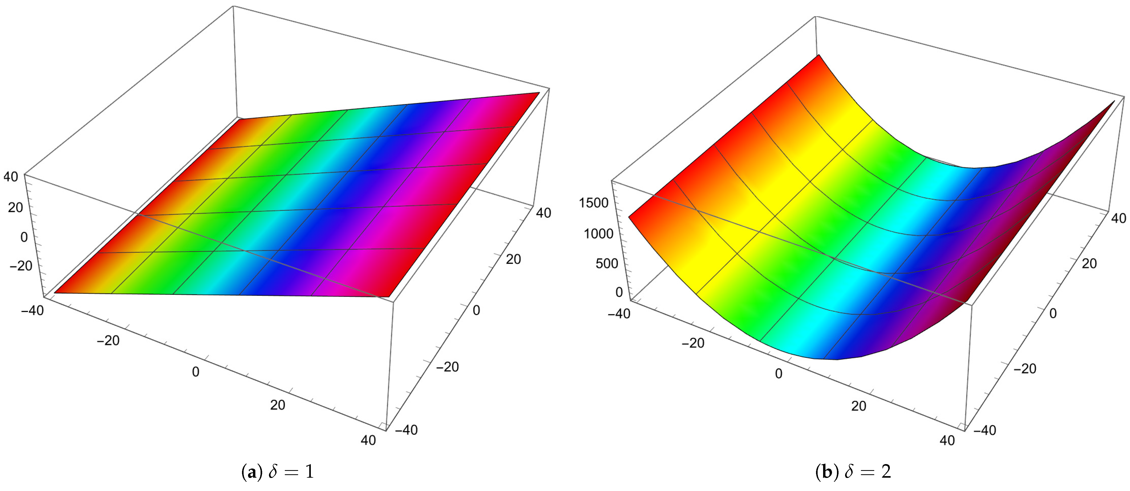
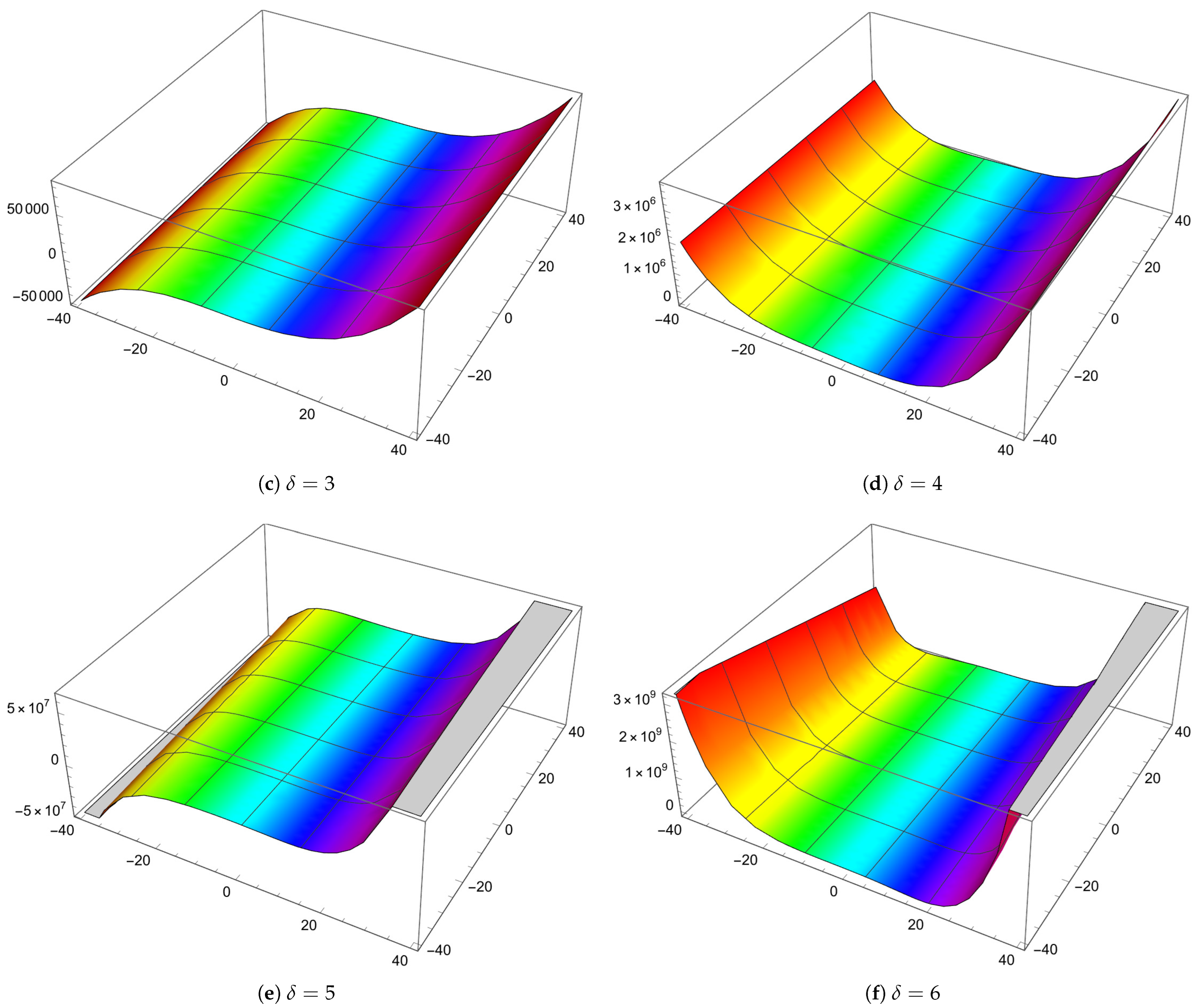
5. Computational and Graphical Representations

This section highlights the advantages of employment numerical computations and explores the distributions of zeros by presenting graphical illustrations of the GGHBelBP ${}_{\mathcal{H}\mathcal{B}el}\mathfrak{B}_{\delta ,\sigma }^{\left(r\right)}({\nu }_1,{\nu }_2,z;\eta )$ for specific values and indices.

The first six terms of the GGHBelBP ${}_{\mathcal{H}\mathcal{B}el}\mathfrak{B}_{\delta ,\sigma }^{\left(r\right)}({\nu }_1,{\nu }_2,z;\eta )$ for $\eta =1$ and $r=3$ are given as

$$\begin{array}{cc}\hfill & {}_{\mathcal{H}\mathcal{B}el}\mathfrak{B}_{0,\sigma }^{\left(3\right)}({\nu }_1,{\nu }_2,z;\eta )=1,\hfill \\ & {}_{\mathcal{H}\mathcal{B}el}\mathfrak{B}_{1,\sigma }^{\left(3\right)}({\nu }_1,{\nu }_2,z;\eta )={\nu }_1+z-{\displaystyle \frac{1}{2}},\hfill \\ & {}_{\mathcal{H}\mathcal{B}el}\mathfrak{B}_{2,\sigma }^{\left(3\right)}({\nu }_1,{\nu }_2,z;\eta )={\nu }_1^2+2{\nu }_{1}z-{\nu }_1+z^2+{\displaystyle \frac{1}{6}},\hfill \\ & {}_{\mathcal{H}\mathcal{B}el}\mathfrak{B}_{3,\sigma }^{\left(3\right)}({\nu }_1,{\nu }_2,z;\eta )={\nu }_1^3+3{\nu }_1^{2}z-{\displaystyle \frac{3{\nu }_1^2}{2}}+3{\nu }_1{z}^2+{\displaystyle \frac{{\nu }_1}{2}}+6\sigma {\nu }_2+z^3+{\displaystyle \frac{3z^2}{2}},\hfill \\ & {}_{\mathcal{H}\mathcal{B}el}\mathfrak{B}_{4,\sigma }^{\left(3\right)}({\nu }_1,{\nu }_2,z;\eta )={\nu }_1^4+4{\nu }_1^{3}z-2{\nu }_1^3+6{\nu }_1^2{z}^2+{\nu }_1^2+24\sigma {\nu }_1{\nu }_2+4{\nu }_1{z}^3+6{\nu }_1{z}^2-12\sigma {\nu }_2\hfill \\ & +24\sigma {\nu }_{2}z+z^4+4z^3+2z^2-{\displaystyle \frac{1}{30}},\hfill \end{array}$$

$$\begin{array}{cc}\hfill & {}_{\mathcal{H}\mathcal{B}el}\mathfrak{B}_{5,\sigma }^{\left(3\right)}({\nu }_1,{\nu }_2,z;\eta )={\nu }_1^5+5{\nu }_1^{4}z-{\displaystyle \frac{5{\nu }_1^4}{2}}+10{\nu }_1^3{z}^2+{\displaystyle \frac{5{\nu }_1^3}{3}}+60\sigma {\nu }_1^2{\nu }_2+10{\nu }_1^2{z}^3+15{\nu }_1^2{z}^2\hfill \\ & -60\sigma {\nu }_1{\nu }_2+120\sigma {\nu }_1{\nu }_{2}z+5{\nu }_1{z}^4+20{\nu }_1{z}^3+10{\nu }_1{z}^2-{\displaystyle \frac{{\nu }_1}{6}}+10\sigma {\nu }_2\hfill \\ & +60\sigma {\nu }_2{z}^2+z^5+{\displaystyle \frac{15z^4}{2}}+{\displaystyle \frac{35z^3}{3}}+{\displaystyle \frac{5z^2}{2}},\hfill \\ \hfill & {}_{\mathcal{H}\mathcal{B}el}\mathfrak{B}_{6,\sigma }^{\left(3\right)}({\nu }_1,{\nu }_2,z;\eta )={\nu }_1^6+6{\nu }_1^{5}z-3{\nu }_1^5+15{\nu }_1^4{z}^2+{\displaystyle \frac{5{\nu }_1^4}{2}}+120\sigma {\nu }_1^3{\nu }_2+20{\nu }_1^3{z}^3+30{\nu }_1^3{z}^2\hfill \\ & -180\sigma {\nu }_1^2{\nu }_2+360\sigma {\nu }_1^2{\nu }_{2}z+15{\nu }_1^2{z}^4+60{\nu }_1^2{z}^3+30{\nu }_1^2{z}^2-{\displaystyle \frac{{\nu }_1^2}{2}}+60\sigma {\nu }_1{\nu }_2\hfill \\ & +360\sigma {\nu }_1{\nu }_2{z}^2+6{\nu }_1{z}^5+45{\nu }_1{z}^4+70{\nu }_1{z}^3+15{\nu }_1{z}^2+360{\sigma }^2{\nu }_2^2+360\sigma {\nu }_2^2\hfill \\ & +120\sigma {\nu }_2{z}^3+180\sigma {\nu }_2{z}^2+z^6+12z^5+{\displaystyle \frac{75z^4}{2}}+30z^3+3z^2+{\displaystyle \frac{1}{42}}.\hfill \end{array}$$

To show the shapes of the GGHBelBP ${}_{\mathcal{H}\mathcal{B}el}\mathfrak{B}_{\delta ,\sigma }^{\left(r\right)}({\nu }_1,{\nu }_2,z;\eta )$ for $\delta =0;1;2;3;4;5, -100\le {\nu }_1\le 100, {\nu }_2=z=\sigma =4, r=3$ and $\eta =1$, Figure 1 is given:

The surface plots of the GGHBelBP ${}_{\mathcal{H}\mathcal{B}el}\mathfrak{B}_{\delta ,\sigma }^{\left(r\right)}({\nu }_1,{\nu }_2,z;\eta )$ for $\delta =1;2;3;4;5;6, -40\le {\nu }_1\le 40, -40\le {\nu }_2\le 40, z=\sigma =4, r=3$ and $\eta =1$ are displayed in Figure 2:

Certain interesting zeros of the GGHBelBP ${}_{\mathcal{H}\mathcal{B}el}\mathfrak{B}_{\delta ,\sigma }^{\left(r\right)}({\nu }_1,{\nu }_2,z;\eta )=0$ for $\eta =1$ and $\delta =80$ are shown in Figure 3.

In Figure 3a, we choose ${\nu }_2=3, z=-3, \sigma =3, r=30$. In Figure 3b, we choose ${\nu }_2=8, z={\displaystyle \frac{1}{8}}, \sigma =2, r=19$. In Figure 3c, we choose ${\nu }_2=8, z={\displaystyle \frac{1}{8}}, \sigma =2, r=11$. In Figure 3d, we choose ${\nu }_2=z=\sigma =r=4$.

Remark 1.

We observe that the zeros of the GGHBelBP ${}_{\mathcal{H}\mathcal{B}el}\mathfrak{B}_{\delta ,\sigma }^{\left(r\right)}({\nu }_1,{\nu }_2,z;\eta )=0$ for $\eta =1$ and $\delta =80$ have the following properties:

• The GGHBelBP ${}_{\mathcal{H}\mathcal{B}el}\mathfrak{B}_{\delta ,\sigma }^{\left(r\right)}({\nu }_1,{\nu }_2,z;\eta )$ of degree δ possess exactly δ zeros.
• Altering the variables, parameters, or indices generates distinct zero distributions and varied graphical configurations.
• The zeros (complex zeros) of GGHBelBP ${}_{\mathcal{H}\mathcal{B}el}\mathfrak{B}_{\delta ,\sigma }^{\left(r\right)}({\nu }_1,{\nu }_2,z;\eta )=0$ exhibit symmetry about the real axis.

The stacking structures of approximation zeros of the GGHBelBP ${}_{\mathcal{H}\mathcal{B}el}\mathfrak{B}_{\delta ,\sigma }^{\left(r\right)}({\nu }_1,{\nu }_2,z;\eta )=0$ for $\eta =1$ and $1\le \delta \le 60$ give 3D structures, which are presented in Figure 4:

The established results in this study offer several practical applications, including the following:

• Fractional Differential Equations: These polynomials can act as effective basis functions for solving fractional PDEs that emerge in diverse scientific and engineering contexts.
• Approximation Theory Insights: Zero distributions generated via Mathematica (Figure 3 and Figure 4) exhibit symmetries and structural patterns with direct utility in advancing approximation-theoretic frameworks.
• Interdisciplinary Relevance: The results intersect with probability theory (through links to Bell polynomials) and combinatorics (via generating functions). Broader implications extend to domains such as fractional control theory and signal processing.

6. Conclusions

The combined use of special polynomials and integral transforms offers a powerful tool to establish a new generalization of hybrid special polynomials. In this study, we used the Euler integral to establish a novel generalized class of hybrid special polynomials, referred to as the generalized Gould–Hopper–Bell–Appell polynomials. By employing the operation method and the Euler integral, in Section 2 and Section 3, we constructed the associated operational definition, generating function, explicit representations, and summation formulas. Additionally, operational representations as well as determinant definitions were derived.

Special members of this generalized family–such as the generalized Gould–Hopper–Bell–Bernoulli polynomials, the generalized Gould–Hopper–Bell–Euler polynomials, and the generalized Gould–Hopper–Bell–Genocchi polynomials—were examined, revealing analogous results for each (Section 4). Furthermore, in Section 5, computational investigations using Mathematica were conducted, to explore the zero distributions and graphical representations of the generalized Gould–Hopper–Bell–Bernoulli polynomials. The visual and numerical analyses offer a more profound understanding of the behavior and characteristics of these polynomials.

In summary, this study extends the utility of the fractional operational approach to create a generalized class of polynomials that generalizes and extends several existing families of special polynomials. The results presented here contribute to the broader field of special functions and polynomial theory by introducing and investigating a new, generalized class of polynomials. This work demonstrates the utility and flexibility of fractional operational methods in constructing and analyzing generalized polynomial structures. The method used in [40] can be considered in further studies. Future research could explore the degenerate forms of the established class in this study, along with their associated applications.

References

1. Gould, H.W.; Hopper, A.T. Operational formulas connected with two generalizations of Hermite polynomials. Duke Math. J. 1962, 29, 51–63. [Google Scholar] [CrossRef]
2. Appell, P.; Kampé de Fériet, J. Fonctions Hypergéométriques et Hypersphériques; Polynômes d’Hermite; Gauthier-Villars: Paris, France, 1926. [Google Scholar]
3. Duran, U.; Araci, S.; Acikgoz, M. Bell-based Bernoulli polynomials with applications. Axioms 2021, 10, 29. [Google Scholar] [CrossRef]
4. Carlitz, L. Some Remarks on the Bell numbers. Fibonacci Quart. 1980, 18, 66–73. [Google Scholar] [CrossRef]
5. Andrews, L.C. Special Functions for Engineers and Applied Mathematics; Macmillan Publishing Company: New York, NY, USA, 1985. [Google Scholar]
6. Anshelevich, M. Appell polynomials and their relatives III. Conditionally free theory. Ill. J. Math. 2009, 53, 39–66. [Google Scholar] [CrossRef]
7. Salminen, P. Optimal stopping, Appell polynomials and Wiener–Hopf factorization. Int. J. Probab. Stoch. Process. 2011, 83, 611–622. [Google Scholar] [CrossRef]
8. Malonek, H.R.; Falcão, M.I. 3D-mappings using monogenic functions. In Numerical Analysis and Applied Mathematics-ICNAAM 2006; Simos, T.E., Psihoyios, G., Tsitouras, C., Eds.; Wiley: Weinheim, Germany, 2006; pp. 615–619. [Google Scholar]
9. Brackx, F.; De Schepper, H.; Lávička, R.; Soucek, V. Gel’fand-Tsetlin Procedure for the Construction of Orthogonal Bases in Hermitean Clifford Analysis. In Numerical Analysis and Applied Mathematics-ICNAAM 2010; Simos, T.E., Psihoyios, G., Tsitouras, C., Eds.; AIP Conference Proceedings, Volume 1281; American Institute of Physics (AIP): Melville, NY, USA, 2010; pp. 1508–1511. [Google Scholar]
10. Lávička, R. Canonical bases for sl (2, C)-modules of spherical monogenics in dimension 3. Arch. Math. Tomus 2010, 46, 339–349. [Google Scholar]
11. Weinberg, S.T. The Quantum Theory of Fields; Cambridge University Press: Cambridge, UK, 1995; Volume 1. [Google Scholar]
12. Fadel, M.; Alatawi, M.S.; Khan, W.A. Two-variable q-Hermite-based Appell polynomials and their applications. Mathematics 2024, 12, 1358. [Google Scholar] [CrossRef]
13. Alyusof, R.; Wani, S.A. Certain properties and applications of μh hybrid special polynomials associated with Appell sequences. Fractal Fract. 2023, 7, 233. [Google Scholar] [CrossRef]
14. Alam, N.; Wani, S.A.; Khan, W.A.; Zaidi, H.N. Investigating the Properties and Dynamic Applications of μh Legendre–Appell Polynomials. Mathematics 2024, 12, 1973. [Google Scholar] [CrossRef]
15. Zayed, M.; Wani, S.A.; Mahnashi, A.M. Certain properties and characterizations of multivariable Hermite-Based Appell polynomials via factorization method. Fractal Fract. 2023, 7, 605. [Google Scholar] [CrossRef]
16. Yasmin, G.; Muhyi, A.; Araci, S. Certain results of q-Sheffer–Appell polynomials. Symmetry 2019, 11, 159. [Google Scholar] [CrossRef]
17. Muhyi, A.; Araci, S. A Note on q-Fubini-Appell Polynomials and Related Properties. J. Funct. Spaces 2021, 2021, 3805809. [Google Scholar] [CrossRef]
18. Fadel, M.; Muhyi, A. On a family of q-modified-Laguerre-Appell polynomials. Arab J. Basic Appl. Sci. 2024, 31, 165–176. [Google Scholar] [CrossRef]
19. Khan, S.; Yasmin, G.; Ahmad, N. A note on truncated exponential-Based Appell polynomials. Bull. Malays. Math. Sci. Soc. 2017, 40, 373–388. [Google Scholar] [CrossRef]
20. Khan, S.; Raza, N.; Ali, M. Finding mixed families of special polynomials associated with Appell sequences. J. Math. Anal. Appl. 2017, 447, 398–418. [Google Scholar] [CrossRef]
21. Yasmin, G.; Muhyi, A. Certain results of hybrid families of special polynomials associated with Appell sequences. Filomat 2019, 33, 3833–3844. [Google Scholar] [CrossRef]
22. Yasmin, G.; Ryoo, C.S.; Islahi, H. A numerical computation of zeros of q-generalized tangent-Appell polynomials. Mathematics 2020, 8, 383. [Google Scholar] [CrossRef]
23. Muhyi, A. A Note on Generalized Bell-Appell Polynomials. Adv. Anal. Appl. Math. 2024, 1, 90–100. [Google Scholar] [CrossRef]
24. Özat, Z.; Özarslan, M.A.; Çekim, B. On Bell based Appell polynomials. Turk. J. Math. 2023, 47, 1099–1128. [Google Scholar] [CrossRef]
25. Khan, S.; Raza, N. General-Appell polynomials within the context of monomiality principle. Int. J. Anal. 2013, 2013, 328032. [Google Scholar] [CrossRef]
26. Al-Jawfi, R.A.; Muhyi, A.; Al-shameri, W.F.H. On generalized class of Bell polynomials associated with geometric applications. Axioms 2024, 13, 73. [Google Scholar] [CrossRef]
27. Assante, D.; Cesarano, C.; Fornaro, C.; Vazquez, L. Higher order and fractional diffusive equations. J. Eng. Sci. Technol. Rev. 2015, 8, 202–204. [Google Scholar] [CrossRef]
28. Dattoli, G. Operational methods, fractional operators and special polynomials. Appl. Math. Comput. 2003, 141, 151–159. [Google Scholar] [CrossRef]
29. Dattoli, G.; Ricci, P.E.; Cesarano, C.; Vazquez, L. Special polynomials and fractional calculus. Math. Comput. Model. 2003, 37, 729–733. [Google Scholar] [CrossRef]
30. Khan, S.; Wani, S.A. Extended Laguerre-Appell polynomials via fractional operators and their determinant forms. Turk. J. Math. 2018, 42, 1686–1697. [Google Scholar] [CrossRef]
31. Yasmin, G.; Muhyi, A. Extended forms of Legendre-Gould-Hopper-Appell polynomials. Adv. Stud. Contemp. Math. 2019, 29, 489–504. [Google Scholar]
32. Khan, S.; Wani, S.A.; Riyasat, M. Study of generalized Legendre-Appell polynomials via fractional operators. TWMS J. Pure Appl. Math. 2020, 11, 144–156. [Google Scholar]
33. Srivastava, H.M.; Manocha, H.L. A Trestise on Generating Functions; Halested Press-Ellis Horwood Limited-Jon Wiely and Sons: New York, NY, USA; Chichester, UK; Srisbane, QLD, Australia; Toronto, ON, Canada, 1984. [Google Scholar]
34. Özarslan, M.A. Unified Apostol-Bernoulli, Euler and Genocchi polynomials. Comput. Math. Appl. 2011, 62, 2452–2462. [Google Scholar] [CrossRef]
35. Khan, N.; Husain, S. Analysis of Bell based Euler polynomials and their application. Int. J. Appl. Comput. Math. 2021, 7, 195. [Google Scholar] [CrossRef]
36. Duran, U.; Acikgoz, M. Bell-based Genocchi polynomials. New Trends Math. Sci. 2021, 9, 50–55. [Google Scholar] [CrossRef]
37. Bildirici, C.; Acikgoz, M.; Araci, S. A note on analogues of tangent polynomials. J. Algebra Number Theory Acad. 2014, 4, 21–29. [Google Scholar]
38. Costabile, F.A.; Longo, E. A determinantal approach to Appell polynomials. J. Comput. Appl. Math. 2010, 234, 1528–1542. [Google Scholar] [CrossRef]
39. Costabile, F.A.; Dell’ Accio, F.; Gualtieri, M.I. A new approach to Bernoulli polynomials. Rend. Mat. Appl. 2006, 26, 1–12. [Google Scholar]
40. Leinartas, E.; Shishkina, O. The Euler-Maclaurin Formula in the Problem of Summation over Lattice Points of a Simplex. J. Sib. Fed. Univ. Math. Phys. 2022, 15, 108–113. [Google Scholar] [CrossRef]
Figure 1. Curves of B δ , σ ( r ) H B e l ( ν 1 , ν 2 , z ; η ) for 100 ν 1 100 ,   ν 2 = z = σ = 4 ,   r = 3 , η = 1 and for δ = 0 (top-left); δ = 1 (top-right); δ = 2 (middle-left); δ = 3 (top-right); δ = 4 (bottom-left); δ = 5 (bottom-right).
Fractalfract 09 00281 g001aFractalfract 09 00281 g001b
Figure 2. Surface plots of B δ , σ ( r ) H B e l ( ν 1 , ν 2 , z ; η ) for 40 ν 1 40 ,   40 ν 2 40 ,   z = σ = 4 ,   r = 3 and η = 1 , and for δ = 1 (a); δ = 2 (b); δ = 3 (c); δ = 4 (d); δ = 5 (e); δ = 6 (f).
Fractalfract 09 00281 g002aFractalfract 09 00281 g002b
Figure 3. Zeros of GGHBelBP B δ , σ ( r ) H B e l ( ν 1 , ν 2 , z ; η ) = 0 for η = 1 , δ = 80 , and different values of ν 2 ,   z ,   σ ,   r .
Fractalfract 09 00281 g003
Figure 4. Stacking structure zeros of GGHBelBP B δ , σ ( r ) H B e l ( ν 1 , ν 2 , z ; η ) = 0 . This figure shows the 3D plot of the zeros of the GGHBelBP B δ , σ ( r ) H B e l ( ν 1 , ν 2 , z ; η ) = 0 for η = 1 and 1 δ 60 .
Fractalfract 09 00281 g004