An Atangana–Baleanu Fractional Derivative Approach to Modeling Diabetes Progression and Optimizing Comorbidity Reduction and Prevention

Abstract

This study presents a fractional-order dynamical model for diabetes progression, formulated by extending an existing obesity model using the Atangana–Baleanu fractional derivative, termed the Atangana–Baleanu Fractional Diabetes Model (ABFDM). We rigorously establish the existence, uniqueness, positivity, and boundedness of solutions, ensuring the model’s epidemiological and biological validity. The Ulam–Hyers $\left(\mathbb{UH}\right)$ stability of the ABFDM is also demonstrated, confirming the system’s robustness against perturbations in initial conditions and parameter uncertainties. Numerical simulations, informed by population data from Saudi Arabia, indicate that increasing treatment coverage fourfold reduces uncontrolled diabetes ($D_U$) by approximately 73% and diabetes with complications ($D_W$) by about 68%. The greatest improvements occur when treatment is increased tenfold, further lowering prediabetes ($D_P$) by approximately 89% and diabetic complications ($D_W$) by about 73%. These results highlight that optimized, targeted interventions effectively control diabetes progression and mitigate the burden of related complications. These findings demonstrate that targeted treatment strategies can effectively mitigate diabetes progression within the fractional-order modeling framework.

1. Introduction

Diabetes mellitus (DM) is a long-term metabolic condition marked by persistently high blood glucose levels, resulting from inadequate insulin production, impaired insulin action, or a combination of both. It stands among the most widespread and rapidly growing non-communicable diseases globally and ranks as the fourth leading cause of mortality worldwide. According to the International Diabetes Federation, an estimated 537 million adults aged 20–79 years were affected by diabetes in 2021, with projections indicating a rise to nearly 783 million by 2045 [1]. The disease burden is highest in the Western Pacific (215 million), South-East Asia (107 million), and the Middle East and North Africa (MENA) regions (85 million), as illustrated in Figure 1 and Figure 2. In the MENA region alone, diabetes prevalence reached 10.5% in 2021 and is anticipated to increase to 12.2% by 2045, underscoring the pressing need for tailored, region-specific prevention and control strategies.

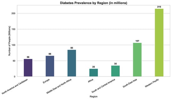
Figure 1. Global diabetes case distribution by region. Prevalence is highest in the Western Pacific and South-East Asia, while burdens remain substantial in Africa and South/Central America, emphasizing the need for region-specific interventions.

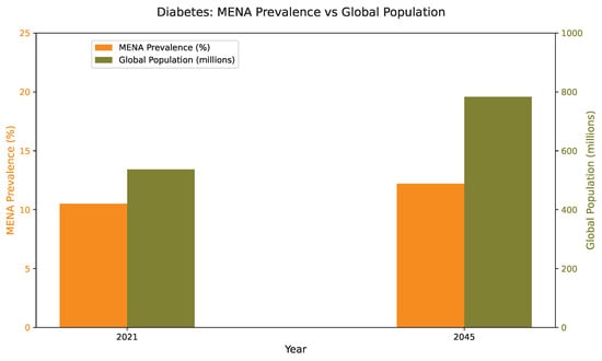
Figure 2. Prevalence of diabetes among adults aged 20–79 years in the Middle East and North Africa (MENA) region compared with global averages, highlighting the projected increase in disease burden from 2021 to 2045.

Recent global reports show that diabetes now affects people of all ages, with a particularly rapid increase among adults. This growing prevalence reflects broader demographic, lifestyle, and nutritional transitions occurring worldwide. In 2022, approximately 14% of adults aged 18 and older were living with diabetes, double the prevalence reported in 1990 (7%). By 2024, an estimated 589 million adults aged 20 to 79 years had diabetes worldwide, representing about 11.1% of this age group, and forecasts indicate that the number could rise to nearly 853 million by 2050 [2]. The burden is greatest in low and middle income countries, where limited access to healthcare and a high proportion of undiagnosed cases contribute to elevated mortality rates. In 2024, diabetes accounted for more than 3.4 million deaths globally, emphasizing its persistent and growing impact on public health.

Building on these global trends, Type 2 diabetes (T2D) represents the predominant form of the disease and is largely associated with insulin resistance resulting from obesity, poor dietary habits, and reduced physical activity. Obesity continues to be the most influential modifiable risk factor, with deaths attributable to elevated body mass index (BMI) increasing from about 238,000 in 1990 to more than 723,000 in 2021 [3]. Huang et al. [3] reported that individuals with obesity have a three to five fold greater likelihood of developing T2D compared with those of normal weight, with women exhibiting a slightly higher relative risk. In many African populations, approximately 61% of individuals with T2D are overweight or obese, reaching up to 85% in certain subregions. Taylor [4] introduced the twin cycle hypothesis, which describes how chronic overnutrition leads to fat accumulation in the liver and pancreas, triggering insulin resistance and beta-cell dysfunction. Complementarily, Chandrasekaran et al. [5] demonstrated that a 5–10% reduction in body weight achieved through dietary changes, physical activity, or pharmacological intervention significantly enhances glycemic control, insulin sensitivity, and lipid metabolism. Collectively, these findings highlight that effective prevention and management of T2D depend on integrated approaches combining obesity control, lifestyle modification, and early targeted interventions.

Given the complex interplay between biological, behavioral, and environmental factors influencing diabetes progression, mathematical modeling has emerged as a vital tool for elucidating disease mechanisms and designing effective control strategies. Through quantitative modeling, researchers can simulate glucose–insulin interactions, predict disease outcomes, and evaluate intervention effectiveness under varying physiological conditions. Jajarmi et al. [6] introduced fractional-order differential models that capture memory and hereditary effects inherent in glucose–insulin regulation, offering more realistic system behavior compared to traditional models. Building upon this, Kouidere et al. [7] expanded the modeling framework by integrating obesity and overweight compartments, showing that managing weight transitions plays a decisive role in lowering diabetes prevalence. Delgado Moya et al. [8] refined these approaches by implementing multi-control strategies to jointly regulate glucose concentration and body weight. Further applications of fractional modeling have explored comorbid conditions: Omame et al. [9] investigated the coupled dynamics of diabetes and tuberculosis using nonsingular Mittag–Leffler kernels, while Mollah et al. [10] analyzed diabetes–COVID-19 co-infection through the Atangana–Baleanu fractional derivative, demonstrating that vaccination and adherence to preventive measures markedly reduce co-infection rates. Together, these contributions underscore the adaptability and growing significance of fractional-order and optimal control modeling in advancing diabetes research and informing clinical and public health interventions.

Building on earlier modeling advances, Youssef et al. [11] developed an optimal control model that stratifies the population by body mass index (BMI) categories, ranging from healthy to obesity classes I–III, while incorporating the dynamics of obesity-related comorbidities. The model guarantees solution positivity and stability, and simulations using the Runge–Kutta and Forward–Backward Sweeping methods showed that prevention-oriented strategies markedly outperform treatment alone. Intensive prevention reduced comorbidity prevalence by over 60%, while combined prevention and treatment interventions achieved reductions exceeding 90%. These results highlight the value of proactive prevention programs in alleviating the dual burden of obesity and diabetes, especially in resource-limited settings.

Extending these modeling efforts, fractional calculus (FC) has emerged as a powerful mathematical framework for capturing the memory and hereditary characteristics inherent in biological systems such as diabetes. Dubey et al. [12] introduced a fractional-order diabetes model employing an exponential kernel, establishing its well-posedness through fixed-point theory and validating its realism using the Homotopy Perturbation Method. Yadav et al. [13] developed a fractional-order diabetes model using the Atangana–Baleanu–Caputo (ABC) derivative. They proved the existence and uniqueness of solutions via Picard’s theorem and used a two-step Lagrange interpolation scheme for numerical analysis. Their results indicated that lower fractional orders increase diabetes prevalence, capturing the system’s memory and hereditary behavior. Khan et al. [14] applied a modified ABFD to an HIV–AIDS system, combining analytical and neural network approaches to explore key interactions among hospitalization, vaccination, and recovery rates. Similarly, Nisar et al. [15] modeled conjunctivitis transmission using a Caputo-type derivative, while Adom-Konadu et al. [16] and Dasumani et al. [17] extended fractional modeling to other infectious diseases, collectively demonstrating that fractional order plays a critical role in shaping disease progression and control effectiveness.

Previous modeling studies, such as that of Youssef et al. [11], formulated an optimal control framework for obesity dynamics stratified by body mass index (BMI) categories and associated comorbidities. However, their model did not explicitly capture the progression from obesity to diabetes and the subsequent stages of diabetic development within a fractional framework. To bridge this gap, the present study extends the obesity model of Youssef et al. [11] into a comprehensive fractional-order system that incorporates additional compartments representing prediabetic, uncontrolled diabetic, controlled diabetic, and diabetic-with-complications states. The proposed model employs the Atangana–Baleanu fractional derivative (ABFD) in the Caputo sense to describe the memory-dependent and hereditary characteristics inherent in diabetes progression allowing the exploration of novel dynamical behaviors and a deeper understanding of the underlying functional space. This formulation strengthens the connection between obesity prevention and diabetes control, enhances the biological realism of fractional modeling, and provides a quantitative framework for assessing the effectiveness of prevention-oriented strategies.

The remainder of this work is organized as follows. Section 2 reviews the fundamental mathematical concepts essential for formulating and analyzing the proposed fractional-order dynamical model. Section 3 introduces the Atangana–Baleanu Fractional Diabetes Model (ABFDM), detailing its formulation, key assumptions, and governing equations. Section 4 investigates the model’s qualitative properties, including existence and uniqueness of solutions, positivity, boundedness, and Ulam–Hyers (UH) stability. Section 5 presents the numerical methods and simulation results, illustrating the impact of fractional-order parameters and treatment strategies on diabetes progression. Finally, Section 6 summarizes the main findings and outlines directions for future research.

2. Essential Preliminaries

This section introduces the essential preliminary framework, encompassing the fundamental definitions of fractional integrals and derivatives, with particular attention devoted to their associated memory kernels. It concludes with an exposition of the recently developed Atangana–Baleanu fractional derivatives (ABFD), characterized by both non-singular and singular kernels, which constitute the theoretical foundation for the proofs of the main results presented in the subsequent sections.

Definition 1

([18]). Let $\wp >0$. The Riemann–Liouville fractional integral (RLFI) of order ℘ for a function $\mathsf{ħ}\left(t\right)$ is defined as

$${}_{0\hspace{1em}}{}^{\mathcal{RL}}\mathbb{I}_t^{\wp }\mathsf{ħ}\left(t\right)={\displaystyle \frac{1}{\Gamma (\wp )}}{\int }_0^t{(t-k)}^{\wp -1}\mathsf{ħ}\left(k\right)dk,$$

(1)

where $\mathsf{ħ}\left(t\right)\in L^1(0,T)$ and $T<\infty$.

Definition 2

([18]). For $0<\wp <1$, the Caputo fractional derivative (CFD) of order ℘ for a function $\mathsf{ħ}\left(t\right)$ is expressed as

$${}_0{}^{\mathcal{C}}\mathbb{D}_t^{\wp }\mathsf{ħ}\left(t\right)={\displaystyle \frac{1}{\Gamma (1-\wp )}}{\int }_0^t{(t-k)}^{-\wp }{\mathsf{ħ}}^{\prime }\left(k\right)dk,$$

(2)

where ${\mathsf{ħ}}^{\prime }\left(t\right)\in L^1(0,T)$ is the first derivative of $\mathsf{ħ}\left(t\right)$.

Definition 3

([19,20,21]). Let $\wp \in (0,1)$. The Atangana Baleanu fractional derivative (ABFD) operator of order ℘ for a function $\mathsf{ħ}\left(t\right)$ in the Caputo sense is defined by

$${}_{0 }{}^{\mathcal{M}}\mathbb{D}_t^{\wp }\mathsf{ħ}\left(t\right)={\displaystyle \frac{\mathcal{A}(\wp )}{1-\wp }}{\int }_0^t{\mathbb{E}}_{\wp }\left(-{\eta }_{\wp }{(t-k)}^{\wp }\right){\mathsf{ħ}}^{\prime }\left(k\right)dk,$$

(3)

where ${\eta }_{\wp }={\displaystyle \frac{\wp }{1-\wp }}$ is a relaxation (scaling) parameter. Here, $\mathcal{A}(\wp )$ is a normalization mapping satisfying $\mathcal{A}\left(0\right)=\mathcal{A}\left(1\right)=1$, ${\mathsf{ħ}}^{\prime }\left(t\right)\in L^1(0,T)$ is the first derivative of $\mathsf{ħ}\left(t\right)$, ${\mathbb{E}}_{\wp }\left(z\right)$ is the Mittag–Leffler function defined by ${\mathbb{E}}_{\wp }\left(z\right)={\sum }_{\xi =0}^{\infty }{\displaystyle \frac{z^{\xi }}{\Gamma (\wp \xi +1)}},$ and $\mathcal{M}$ denotes the Atangana Baleanu operator in the Caputo sense.

Remark 1.

• In Definitions 2 and 3, at $\wp =0$ we define the operators directly as ${}_0{}^{\mathcal{C}}\mathbb{D}_t^0\mathsf{ħ}\left(t\right)={}_{0 }{}^{\mathcal{M}}\mathbb{D}_t^0\mathsf{ħ}\left(t\right)=\mathsf{ħ}\left(t\right)-\mathsf{ħ}\left(0\right)$, while at $\wp \to 1^{-}$ the operators are defined by the limiting process ${}_0{}^{\mathcal{C}}\mathbb{D}_t^1\mathsf{ħ}\left(t\right)={}_{0 }{}^{\mathcal{M}}\mathbb{D}_t^1\mathsf{ħ}\left(t\right)={\mathsf{ħ}}^{\prime }\left(t\right)$. This clarifies that the fractional order interval can be extended to $[0,1]$, with $\wp =0$ defined directly and $\wp =1$ interpreted as a limit.
• The Caputo-type Atangana–Baleanu fractional derivative (ABFD) employs the parameter ${\eta }_{\wp }={\displaystyle \frac{\wp }{1-\wp }}$ to scale its Mittag–Leffler kernel ${\mathbb{E}}_{\wp }\left(-{\eta }_{\wp }{(t-k)}^{\wp }\right)$. This parameter ensures that the kernel remains properly normalized and that the memory term transitions smoothly between short and long term effects. In particular, ${\eta }_{\wp }$ acts as a relaxation rate: for small ℘ it provides slow decay (long memory), while for $\wp \to 1$ it grows large, concentrating the kernel near $t=k$ and recovering the classical first-order derivative. Therefore, ${\eta }_{\wp }$ controls the influence of past states in a way that preserves consistency with the integral formulation and captures both Markovian and non-Markovian dynamics.

Definition 4

([19,20]). The Atangana–Baleanu fractional integral (ABFI) operator corresponding to Definition 3 is given by

$${}_{0 }{}^{\mathcal{M}}\mathbb{I}_t^{\wp }\mathsf{ħ}\left(t\right)={\displaystyle \frac{1-\wp }{\mathcal{A}(\wp )}}\mathsf{ħ}\left(t\right)+{\displaystyle \frac{\wp }{\mathcal{A}(\wp )\Gamma (\wp )}}{\int }_0^t{(t-k)}^{\wp -1}\mathsf{ħ}\left(k\right)dk.$$

(4)

Lemma 1

([19,20,21]). Let $\wp \in (0,1)$ and suppose that ${\mathsf{ħ}}^{\prime }\left(t\right)\in L^1(0,T)$. Then, for the Atangana–Baleanu fractional integral (ABFI) operator ${}_{0 }{}^{\mathcal{M}}\mathbb{I}_t^{\wp }$ defined in Definition 4 and the corresponding Atangana–Baleanu fractional derivative (ABFD) operator ${}_{0 }{}^{\mathcal{M}}\mathbb{D}_t^{\wp }$ defined in Definition 3, we have

$${}_{0 }{}^{\mathcal{M}}\mathbb{I}_t^{\wp }\left({}_{0 }{}^{\mathcal{M}}\mathbb{D}_t^{\wp }\mathsf{ħ}\left(t\right)\right)=\mathsf{ħ}\left(t\right)-\mathsf{ħ}\left(0\right).$$

Lemma 2

([18,19,20]). The Laplace transform of the Atangana–Baleanu fractional derivative (ABFD) defined in Definition 3 is given by

$$\mathcal{L}\left\{{}_{0 }{}^{\mathcal{M}}\mathbb{D}_t^{\wp }\mathsf{ħ}\left(t\right)\right\}\left(q\right)={\displaystyle \frac{\mathcal{A}(\wp )\left(q^{\wp }\mathcal{L}\{\mathsf{ħ}\left(t\right)\}\left(q\right)-q^{\wp -1}\mathsf{ħ}\left(0\right)\right)}{\wp +(1-\wp )q^{\wp }}}.$$

(5)

Remark 2.

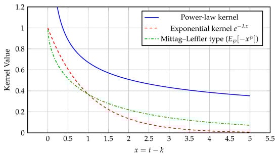
Figure 3 compares three representative kernels used in fractional operators:

Figure 3. Comparison of power-law, exponential, and Mittag–Leffler kernels illustrating fractional memory decay for $\wp =0.6$ and $\lambda =1$.

• The power-law kernel, typically of the form ${(t-k)}^{-\wp }$ (or ${(t-k)}^{\wp -1}$ for the integral form), used in the Riemann–Liouville and Caputo formulations, represents long-memory processes with slow algebraic decay, introducing memory effects into the system being studied and reflecting its dependence on prior states.
• The exponential kernel $e^{-\lambda (t-k)}$, used in the Caputo–Fabrizio derivative, represents short-memory systems with rapid exponential fading, where $\lambda >0$ is the relaxation (decay) rate controlling how quickly past states lose influence.
• The Mittag–Leffler kernel ${\mathbb{E}}_{\wp }\left(-\lambda {(t-k)}^{\wp }\right)$, used in the Atangana–Baleanu derivative, provides an intermediate behavior bridging the power-law and exponential cases, where $\lambda >0$ controls the transition rate between these two memory regimes.

These kernels capture distinct memory effects in fractional systems. In applications such as diabetes modeling, the Mittag–Leffler kernel enables a more realistic description of glucose–insulin interactions, reflecting memory effects that decay at an intermediate rate between exponential and power-law behaviors.

Definition 5

([22]). Let ${\mathcal{T}:(\mathfrak{X},\parallel ·\parallel }_{\mathfrak{X}}{) \to (\mathfrak{Y},\parallel ·\parallel }_{\mathfrak{Y}})$ be a mapping between normed spaces. We say that $\mathcal{T}$ is Hyers–Ulam stable if there exists a constant $\kappa >0$ such that, for every $\epsilon >0$, any $y\in Range\left(\mathcal{T}\right)$, and any $x\in \mathfrak{X}$ with ${\parallel y-\mathcal{T}\left(x\right)\parallel }_{\mathfrak{Y}}<\epsilon$, there exists $x_0\in \mathfrak{X}$ such that $\mathcal{T}\left(x_0\right)=y$ and $\parallel x_0{-x\parallel }_{\mathfrak{X}}<\kappa \epsilon$.

In what follows, let $\mathcal{J}=[0,T]$ with $T<\infty$, and consider the Banach space $\mathbb{M}\left(\mathcal{J}\right)$ of continuous functions on $\mathcal{J}$, equipped with the norm $\parallel x\parallel :={sup}_{t\in \mathcal{J}}\left|x\left(t\right)\right|,x\in \mathbb{M}\left(\mathcal{J}\right).$ For a given $n\in \mathbb{N}$, we define the product space $\mathcal{Q}:=\mathbb{M}{\left(\mathcal{J}\right)}^n,$ and denote a vector in $\mathcal{Q}$ by $\mathbf{X}={(x_1,x_2,\dots ,x_n)}^{\top }\in \mathcal{Q}.$ The space $\mathcal{Q}$ is equipped with the norm ${\parallel \mathbf{X}\parallel }_{\mathcal{Q}}:={max}_{1\le i\le n}\parallel x_i\parallel .$ This functional framework provides a suitable setting for analyzing the fractional-order compartmental model introduced in next sections.

3. Atangana–Baleanu Fractional Diabetes Model (ABFDM)

In this section, we construct a fractional compartmental model to describe the progression of diabetes within a population. The model captures the transition of individuals from a healthy state to the onset of diabetes and forms the foundation for an optimal control framework aimed at identifying the most effective intervention strategies. To define the obesity-related compartments, the model adopts the Body Mass Index (BMI) classifications provided by the CDC [23]. BMI is calculated as an individual’s weight in kilograms divided by the square of their height in meters, with standardized categories applied uniformly to adults aged 20 years and above, regardless of sex, race, or ethnicity. According to these classifications, individuals are categorized as underweight (BMI less than 18.5), normal weight (BMI from 18.5 up to but not including 25), overweight (BMI from 25 up to but not including 30), and obese (BMI of 30 or greater). The obese category is further subdivided into three classes: Class 1 obesity (BMI from 30 to less than 35), Class 2 obesity (BMI from 35 to less than 40), and Class 3 obesity, also referred to as severe obesity (BMI of 40 or higher). These BMI-based classifications inform the compartmental structure of the model, allowing for a more nuanced representation of how different obesity levels influence the development and progression of diabetes.

This work extends the compartmental model previously introduced by Youssef et al. [11], which partitioned the total population into six compartments:

$$\mathbf{N}\left(t\right)=H\left(t\right)+V\left(t\right)+O_1\left(t\right)+O_2\left(t\right)+O_3\left(t\right)+C\left(t\right),$$

where $H\left(t\right)$ represents healthy individuals, $V\left(t\right)$ the overweight class, $O_1\left(t\right)$, $O_2\left(t\right)$, and $O_3\left(t\right)$ correspond to obesity classes I, II, and III, respectively, and $C\left(t\right)$ denotes individuals with comorbidities. That framework was constructed under the assumptions of a constant recruitment rate, BMI-driven obesity dynamics, natural and comorbidity-related mortality, and homogeneous mixing within the population.

In the current study, we incorporate the dynamics of diabetes into the population structure. Specifically, we consider the total population at time t, denoted by $\mathbf{N}\left(t\right)$, to be subdivided into the following distinct epidemiological compartments:

$$\mathbf{N}\left(t\right)=H\left(t\right)+V\left(t\right)+O_1\left(t\right)+O_2\left(t\right)+O_3\left(t\right)+D_P\left(t\right)+D_U\left(t\right)+D_C\left(t\right)+D_W\left(t\right),$$

(6)

where $H\left(t\right)$ corresponds to healthy individuals, $V\left(t\right)$ denotes those who are overweight, and $O_1\left(t\right)$, $O_2\left(t\right)$, and $O_3\left(t\right)$ represent individuals in obesity classes I, II, and III, respectively. The diabetic progression is captured through the compartments $D_P\left(t\right)$ for prediabetic individuals, $D_U\left(t\right)$ for those with uncontrolled diabetes, $D_C\left(t\right)$ for individuals with controlled diabetes, and $D_W\left(t\right)$ for diabetic individuals suffering from comorbid conditions.

This extended model provides a more detailed representation of the interactions between obesity and diabetes by incorporating additional compartments related to diabetic states. The refined structure sets the stage for subsequent mathematical analysis, including the formulation of a fractional-order model and the investigation of qualitative dynamics and optimal intervention strategies.

In addition to the assumptions established in the previous model [11], the current work introduces the following diabetes-specific considerations to support the expanded compartmental structure. These assumptions form the foundation of the proposed fractional-order model illustrated in the Figure 4.

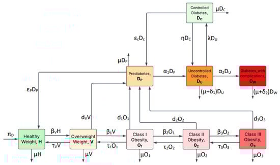
Figure 4. Diabetes compartmental model showing the transitions among H, V, $O_1$, $O_2$, $O_3$, $D_P$, $D_U$, $D_C$, and $D_W$.

(i)

Individuals born to diabetic parents or those with a family history of diabetes are considered genetically predisposed to the disease. Although they are initially classified within the healthy weight compartment, this genetic susceptibility increases their likelihood of transitioning to overweight or prediabetic states over time.

(ii)

There are various non-genetic factors, including insulin resistance, autoimmune disorders, hormonal imbalances, pancreatic damage, and prolonged use of certain medications such as corticosteroids and antiretrovirals, that increase the risk of diabetes and influence transitions into diabetic and prediabetic compartments within the model.

(iii)

Treatment interruption in diabetes management is often attributed to systemic limitations such as, but not limited to, insufficient access to healthcare services and essential resources as well as behavioral and lifestyle challenges; including non-adherence, lack of social support, and economic hardship.

(iv)

Type 2 diabetes constitutes the predominant form of the disease, accounting for 90% to 95% of all diagnosed cases.

Based on the preceding assumptions and Figure 4, we derive the following fractional system of differential Equation (7) using the Atangana–Baleanu fractional derivative (ABFD) of order ℘ in the Caputo sense, as follows:

$$\left\{\begin{array}{cc}\hfill {}_{0 }{}^{\mathcal{M}}\mathbb{D}_t^{\wp }H\left(t\right)& ={\Pi }_D+{\tau }_{v}V\left(t\right)+{ϵ}_P{D}_P\left(t\right)-({\beta }_v+\mu )H\left(t\right),\hfill \\ \hfill {}_{0 }{}^{\mathcal{M}}\mathbb{D}_t^{\wp }V\left(t\right)& ={\beta }_{v}H\left(t\right)+{\tau }_1{O}_1\left(t\right)-(d_v+{\beta }_1+{\tau }_v+\mu )V\left(t\right),\hfill \\ \hfill {}_{0 }{}^{\mathcal{M}}\mathbb{D}_t^{\wp }{O}_1\left(t\right)& ={\beta }_{1}V\left(t\right)+{\tau }_2{O}_2\left(t\right)-({\beta }_2+{\tau }_1+d_1+\mu )O_1\left(t\right),\hfill \\ \hfill {}_{0 }{}^{\mathcal{M}}\mathbb{D}_t^{\wp }{O}_2\left(t\right)& ={\beta }_2{O}_1\left(t\right)+{\tau }_3{O}_3\left(t\right)-({\beta }_3+{\tau }_2+d_2+\mu )O_2\left(t\right),\hfill \\ \hfill {}_{0 }{}^{\mathcal{M}}\mathbb{D}_t^{\wp }{O}_3\left(t\right)& ={\beta }_3{O}_2\left(t\right)-({\tau }_3+d_3+\mu )O_3\left(t\right),\hfill \\ \hfill {}_{0 }{}^{\mathcal{M}}\mathbb{D}_t^{\wp }{D}_P\left(t\right)& =d_{v}V\left(t\right)+d_1{O}_1\left(t\right)+d_2{O}_2\left(t\right)+d_3{O}_3\left(t\right)+{ϵ}_C{D}_C\left(t\right)-({ϵ}_P+{\alpha }_1+\mu )D_P\left(t\right),\hfill \\ \hfill {}_{0 }{}^{\mathcal{M}}\mathbb{D}_t^{\wp }{D}_U\left(t\right)& ={\alpha }_1{D}_P\left(t\right)+\eta D_C\left(t\right)-(\lambda +{\alpha }_2+{\delta }_1+\mu )D_U\left(t\right),\hfill \\ \hfill {}_{0 }{}^{\mathcal{M}}\mathbb{D}_t^{\wp }{D}_C\left(t\right)& =\lambda D_U\left(t\right)-(\eta +{ϵ}_C+\mu )D_C\left(t\right),\hfill \\ \hfill {}_{0 }{}^{\mathcal{M}}\mathbb{D}_t^{\wp }{D}_W\left(t\right)& ={\alpha }_2{D}_U\left(t\right)-(\mu +{\delta }_2)D_W\left(t\right),\hfill \end{array}\right.$$

(7)

where $\mathcal{M}$ denotes the Atangana–Baleanu operator in the Caputo sense. The initial conditions are $H\left(0\right)=H_0,V\left(0\right)=V_0,O_1\left(0\right)=O_{1,0},O_2\left(0\right)=O_{2,0},O_3\left(0\right)=O_{3,0},D_P\left(0\right)=D_{P,0},D_U\left(0\right)=D_{U,0},D_C\left(0\right)=D_{C,0},D_W\left(0\right)=D_{W,0}$. The parameter definitions for the ABFDM in Equation (7) appear in Table 1.

Table 1. Parameters (units: ${\mathrm{year}}^{-1}$).

Parameter	Meaning	Value	Source
${\Pi }_D$	Recruitment rate	0.01335	[24]
${\beta }_v$	Rate of becoming overweight	0.13	[25]
${\beta }_1$	Rate of becoming obese stage 1	0.12	[25]
${\beta }_2$	Rate of becoming obese stage 2	0.10	Assumed
${\beta }_3$	Rate of becoming obese stage 3	0.08	Assumed
$d_v$	Prediabetes acquisition rate for overweight	0.0392	[26]
$d_1$	Prediabetes acquisition rate for obese stage 1	0.33	[27]
$d_2$	Prediabetes acquisition rate for obese stage 2	0.38	[27]
$d_3$	Prediabetes acquisition rate for obese stage 3	0.44	[27]
${\tau }_v$	Treatment rate for overweight	0.09	[28]
${\tau }_1$	Treatment rate for obese stage 1	0.08	[28]
${\tau }_2$	Treatment rate for obese stage 2	0.07	Assumed
${\tau }_3$	Treatment rate for obese stage 3	0.06	Assumed
${\delta }_1$	Uncontrolled diabetes induced mortality rate	0.136	[29]
${\delta }_2$	Diabetes with complications induced mortality rate	0.1225	[30]
$\mu$	Natural mortality rate	0.03	[24]
${\alpha }_1$	Progression rate from $D_P$ to $D_U$	0.025	[31]
${\alpha }_2$	Progression rate from $D_U$ to $D_W$	0.37	[32]
$\lambda$	Treatment rate for diabetes	0.41	[33]
$\eta$	Dropping-off rate of diabetes treatment	0.04–0.19	[34]
${ϵ}_C$	Recovery rate from $D_C$	0.016	[35]
${ϵ}_P$	Recovery rate from prediabetes	0.12	[36]

Remark 3.

(1)

The Caputo-type Atangana–Baleanu (AB) fractional derivative is employed here for its non-singular Mittag–Leffler kernel, which accurately represents memory effects in metabolic and diabetic dynamics. This kernel transitions smoothly between short and long term memory, capturing accumulated physiological interactions such as those between glucose and insulin. The parameter ${\eta }_{\wp }$ provides flexibility to fit physiological data, enabling the model to reflect progressive disease development and intervention impacts more precisely than standard derivatives. Unlike other fractional formulations, the AB Caputo derivative avoids singular behavior, preserves physically consistent relaxation dynamics, and reduces to the classical derivative for integer orders, offering a robust and biologically meaningful modeling framework.

(2)

The parameters listed in Table 1 capture key biological and epidemiological processes driving the relationship between obesity and diabetes in the Atangana–Baleanu Fractional Diabetes Model (ABFDM). The recruitment rate ${\Pi }_D$ balances natural mortality μ to maintain population levels. Transition rates ${\beta }_v$, ${\beta }_1$, ${\beta }_2$, and ${\beta }_3$ govern movement between different BMI categories, decreasing as obesity worsens, while treatment rates ${\tau }_v$, ${\tau }_1$, ${\tau }_2$, and ${\tau }_3$ reflect efforts to return individuals to previous healthier states, also declining with obesity severity. Prediabetes acquisition rates $d_v$, $d_1$, $d_2$, and $d_3$ rise with BMI, indicating higher metabolic risk in obese groups. Parameters ${\alpha }_1$ and ${\alpha }_2$ control disease progression through diabetic stages, while λ, η, ${ϵ}_P$, and ${ϵ}_C$ relate to treatment dynamics and recovery. Mortality rates ${\delta }_1$ and ${\delta }_2$ reflect diabetes-related deaths, with ${\delta }_2>{\delta }_1$ indicative of greater risk in complicated cases. The fractional order ℘ adds a memory effect, integrating past states into the current model. Together, these parameters provide a biologically sound basis for studying the model’s behavior and designing effective interventions.

4. Dynamics and Qualitative Properties of the Proposed ABFDM

4.1. Existence and Uniqueness Results for the ABFDM

In this subsection, we establish that the ABFDM (7) is well-posed by proving the existence and uniqueness of its solution under suitable sufficient conditions. Now, applying the ABFI operator (4) to both sides of the ABFDM (7) gives

$$\left\{\begin{array}{cc}\hfill H\left(t\right)& =H_0+{}_{0 }{}^{\mathcal{M}}\mathbb{I}_t^{\wp }\left\{{\Pi }_D+{\tau }_{v}V\left(t\right)+{ϵ}_P{D}_P\left(t\right)-({\beta }_v+\mu )H\left(t\right)\right\},\hfill \\ \hfill V\left(t\right)& =V_0+{}_{0 }{}^{\mathcal{M}}\mathbb{I}_t^{\wp }\left\{{\beta }_{v}H\left(t\right)+{\tau }_1{O}_1\left(t\right)-(d_v+{\beta }_1+{\tau }_v+\mu )V\left(t\right)\right\},\hfill \\ \hfill O_1\left(t\right)& =O_{1,0}+{}_{0 }{}^{\mathcal{M}}\mathbb{I}_t^{\wp }\left\{{\beta }_{1}V\left(t\right)+{\tau }_2{O}_2\left(t\right)-({\beta }_2+{\tau }_1+d_1+\mu )O_1\left(t\right)\right\},\hfill \\ \hfill O_2\left(t\right)& =O_{2,0}+{}_{0 }{}^{\mathcal{M}}\mathbb{I}_t^{\wp }\left\{{\beta }_2{O}_1\left(t\right)+{\tau }_3{O}_3\left(t\right)-({\beta }_3+{\tau }_2+d_2+\mu )O_2\left(t\right)\right\},\hfill \\ \hfill O_3\left(t\right)& =O_{3,0}+{}_{0 }{}^{\mathcal{M}}\mathbb{I}_t^{\wp }\left\{{\beta }_3{O}_2\left(t\right)-({\tau }_3+d_3+\mu )O_3\left(t\right)\right\},\hfill \\ \hfill D_P\left(t\right)& =D_{P,0}+{}_{0 }{}^{\mathcal{M}}\mathbb{I}_t^{\wp }\left\{d_{v}V\left(t\right)+d_1{O}_1\left(t\right)+d_2{O}_2\left(t\right)+d_3{O}_3\left(t\right)+{ϵ}_C{D}_C\left(t\right)-({ϵ}_P+{\alpha }_1+\mu )D_P\left(t\right)\right\},\hfill \\ \hfill D_U\left(t\right)& =D_{U,0}+{}_{0 }{}^{\mathcal{M}}\mathbb{I}_t^{\wp }\left\{{\alpha }_1{D}_P\left(t\right)+\eta D_C\left(t\right)-(\lambda +{\alpha }_2+{\delta }_1+\mu )D_U\left(t\right)\right\},\hfill \\ \hfill D_C\left(t\right)& =D_{C,0}+{}_{0 }{}^{\mathcal{M}}\mathbb{I}_t^{\wp }\left\{\lambda D_U\left(t\right)-(\eta +{ϵ}_C+\mu )D_C\left(t\right)\right\},\hfill \\ \hfill D_W\left(t\right)& =D_{W,0}+{}_{0 }{}^{\mathcal{M}}\mathbb{I}_t^{\wp }\left\{{\alpha }_2{D}_U\left(t\right)-(\mu +{\delta }_2)D_W\left(t\right)\right\}.\hfill \end{array}\right.$$

(8)

Let $\mathbf{X}\left(t\right)={\left(H\left(t\right),V\left(t\right),O_1\left(t\right),O_2\left(t\right),O_3\left(t\right),D_P\left(t\right),D_U\left(t\right),D_C\left(t\right),D_W\left(t\right)\right)}^{\top }\in \mathcal{Q},n=9,$ and consider the operators ${\mathbf{L}}_j:\mathcal{Q}\times \mathcal{J}\to \mathbb{M}\left(\mathcal{J}\right),j=1,2,\dots ,9,$ defined in (9). We then define the corresponding vector operator $\mathbf{L}(\mathbf{X}\left(t\right),t)={\left({\mathbf{L}}_1(\mathbf{X}\left(t\right),t),{\mathbf{L}}_2(\mathbf{X}\left(t\right),t),\dots ,{\mathbf{L}}_9(\mathbf{X}\left(t\right),t)\right)}^{\top }\in \mathcal{Q}.$

$$\left\{\begin{array}{cc}\hfill {\mathbf{L}}_1(\mathbf{X}\left(t\right),t)& ={\Pi }_D+{\tau }_{v}V\left(t\right)+{ϵ}_P{D}_P\left(t\right)-({\beta }_v+\mu )H\left(t\right),\hfill \\ \hfill {\mathbf{L}}_2(\mathbf{X}\left(t\right),t)& ={\beta }_{v}H\left(t\right)+{\tau }_1{O}_1\left(t\right)-(d_v+{\beta }_1+{\tau }_v+\mu )V\left(t\right),\hfill \\ \hfill {\mathbf{L}}_3(\mathbf{X}\left(t\right),t)& ={\beta }_{1}V\left(t\right)+{\tau }_2{O}_2\left(t\right)-({\beta }_2+{\tau }_1+d_1+\mu )O_1\left(t\right),\hfill \\ \hfill {\mathbf{L}}_4(\mathbf{X}\left(t\right),t)& ={\beta }_2{O}_1\left(t\right)+{\tau }_3{O}_3\left(t\right)-({\beta }_3+{\tau }_2+d_2+\mu )O_2\left(t\right),\hfill \\ \hfill {\mathbf{L}}_5(\mathbf{X}\left(t\right),t)& ={\beta }_3{O}_2\left(t\right)-({\tau }_3+d_3+\mu )O_3\left(t\right),\hfill \\ \hfill {\mathbf{L}}_6(\mathbf{X}\left(t\right),t)& =d_{v}V\left(t\right)+d_1{O}_1\left(t\right)+d_2{O}_2\left(t\right)+d_3{O}_3\left(t\right)+{ϵ}_C{D}_C\left(t\right)-({ϵ}_P+{\alpha }_1+\mu )D_P\left(t\right),\hfill \\ \hfill {\mathbf{L}}_7(\mathbf{X}\left(t\right),t)& ={\alpha }_1{D}_P\left(t\right)+\eta D_C\left(t\right)-(\lambda +{\alpha }_2+{\delta }_1+\mu )D_U\left(t\right),\hfill \\ \hfill {\mathbf{L}}_8(\mathbf{X}\left(t\right),t)& =\lambda D_U\left(t\right)-(\eta +{ϵ}_C+\mu )D_C\left(t\right),\hfill \\ \hfill {\mathbf{L}}_9(\mathbf{X}\left(t\right),t)& ={\alpha }_2{D}_U\left(t\right)-(\mu +{\delta }_2)D_W\left(t\right).\hfill \end{array}\right.$$

(9)

From Definition 4, Equation (8) can now be rewritten as

$$\left\{\begin{array}{cc}\hfill H\left(t\right)& =H_0+{\displaystyle \frac{1-\wp }{\mathcal{A}(\wp )}}{\mathbf{L}}_1(\mathbf{X}\left(t\right),t)+{\displaystyle \frac{\wp }{\mathcal{A}(\wp )\Gamma (\wp )}}{\int }_0^t{(t-\psi )}^{\wp -1}{\mathbf{L}}_1(\mathbf{X}\left(\psi \right),\psi )d\psi ,\hfill \\ \hfill V\left(t\right)& =V_0+{\displaystyle \frac{1-\wp }{\mathcal{A}(\wp )}}{\mathbf{L}}_2(\mathbf{X}\left(t\right),t)+{\displaystyle \frac{\wp }{\mathcal{A}(\wp )\Gamma (\wp )}}{\int }_0^t{(t-\psi )}^{\wp -1}{\mathbf{L}}_2(\mathbf{X}\left(\psi \right),\psi )d\psi ,\hfill \\ \hfill O_1\left(t\right)& =O_{1,0}+{\displaystyle \frac{1-\wp }{\mathcal{A}(\wp )}}{\mathbf{L}}_3(\mathbf{X}\left(t\right),t)+{\displaystyle \frac{\wp }{\mathcal{A}(\wp )\Gamma (\wp )}}{\int }_0^t{(t-\psi )}^{\wp -1}{\mathbf{L}}_3(\mathbf{X}\left(\psi \right),\psi )d\psi ,\hfill \\ \hfill O_2\left(t\right)& =O_{2,0}+{\displaystyle \frac{1-\wp }{\mathcal{A}(\wp )}}{\mathbf{L}}_4(\mathbf{X}\left(t\right),t)+{\displaystyle \frac{\wp }{\mathcal{A}(\wp )\Gamma (\wp )}}{\int }_0^t{(t-\psi )}^{\wp -1}{\mathbf{L}}_4(\mathbf{X}\left(\psi \right),\psi )d\psi ,\hfill \\ \hfill O_3\left(t\right)& =O_{3,0}+{\displaystyle \frac{1-\wp }{\mathcal{A}(\wp )}}{\mathbf{L}}_5(\mathbf{X}\left(t\right),t)+{\displaystyle \frac{\wp }{\mathcal{A}(\wp )\Gamma (\wp )}}{\int }_0^t{(t-\psi )}^{\wp -1}{\mathbf{L}}_5(\mathbf{X}\left(\psi \right),\psi )d\psi ,\hfill \\ \hfill D_P\left(t\right)& =D_{P,0}+{\displaystyle \frac{1-\wp }{\mathcal{A}(\wp )}}{\mathbf{L}}_6(\mathbf{X}\left(t\right),t)+{\displaystyle \frac{\wp }{\mathcal{A}(\wp )\Gamma (\wp )}}{\int }_0^t{(t-\psi )}^{\wp -1}{\mathbf{L}}_6(\mathbf{X}\left(\psi \right),\psi )d\psi ,\hfill \\ \hfill D_U\left(t\right)& =D_{U,0}+{\displaystyle \frac{1-\wp }{\mathcal{A}(\wp )}}{\mathbf{L}}_7(\mathbf{X}\left(t\right),t)+{\displaystyle \frac{\wp }{\mathcal{A}(\wp )\Gamma (\wp )}}{\int }_0^t{(t-\psi )}^{\wp -1}{\mathbf{L}}_7(\mathbf{X}\left(\psi \right),\psi )d\psi ,\hfill \\ \hfill D_C\left(t\right)& =D_{C,0}+{\displaystyle \frac{1-\wp }{\mathcal{A}(\wp )}}{\mathbf{L}}_8(\mathbf{X}\left(t\right),t)+{\displaystyle \frac{\wp }{\mathcal{A}(\wp )\Gamma (\wp )}}{\int }_0^t{(t-\psi )}^{\wp -1}{\mathbf{L}}_8(\mathbf{X}\left(\psi \right),\psi )d\psi ,\hfill \\ \hfill D_W\left(t\right)& =D_{W,0}+{\displaystyle \frac{1-\wp }{\mathcal{A}(\wp )}}{\mathbf{L}}_9(\mathbf{X}\left(t\right),t)+{\displaystyle \frac{\wp }{\mathcal{A}(\wp )\Gamma (\wp )}}{\int }_0^t{(t-\psi )}^{\wp -1}{\mathbf{L}}_9(\mathbf{X}\left(\psi \right),\psi )d\psi .\hfill \end{array}\right.$$

(10)

Let $H\left(t\right),\overline{H}\left(t\right)\in \mathbb{M}\left(\mathcal{J}\right)$ be two functions such that $\mathbf{X}\left(t\right)$ and $\overline{\mathbf{X}}\left(t\right)$ differ only in their first components. Then, we have

$$∥{\mathbf{L}}_1(\mathbf{X}\left(t\right),t)-{\mathbf{L}}_1(\overline{\mathbf{X}}\left(t\right),t)∥\le {\mathsf{\ell }}_1∥H-\overline{H}∥,\mathrm{where}{\mathsf{\ell }}_1={\beta }_v+\mu .$$

(11)

Hence, ${\mathbf{L}}_1$ is ${\mathsf{\ell }}_1$-Lipschitz continuous with respect to the variable H.

Similarly, for each $j=2,3,\dots ,9$, let $\mathbf{X}\left(t\right),\overline{\mathbf{X}}\left(t\right)\in \mathcal{Q}$ be two elements that differ only in their jth components $x_j$ and ${\overline{x}}_j$ respectively. Then, one can verify that

$$∥{\mathbf{L}}_j(\mathbf{X}\left(t\right),t)-{\mathbf{L}}_j(\overline{\mathbf{X}}\left(t\right),t)∥\le {\mathsf{\ell }}_j∥x_j-{\overline{x}}_j∥,$$

(12)

where the corresponding Lipschitz constants ${\mathsf{\ell }}_j$ are given by

$$\begin{array}{cccc}\hfill {\mathsf{\ell }}_2& =d_v+{\beta }_1+{\tau }_v+\mu ,\hfill & \hfill {\mathsf{\ell }}_3& ={\beta }_2+{\tau }_1+d_1+\mu ,\hfill \\ \hfill {\mathsf{\ell }}_4& ={\beta }_3+{\tau }_2+d_2+\mu ,\hfill & \hfill {\mathsf{\ell }}_5& ={\tau }_3+d_3+\mu ,\hfill \\ \hfill {\mathsf{\ell }}_6& ={ϵ}_P+{\alpha }_1+\mu ,\hfill & \hfill {\mathsf{\ell }}_7& =\lambda +{\alpha }_2+{\delta }_1+\mu ,\hfill \\ \hfill {\mathsf{\ell }}_8& =\eta +{ϵ}_C+\mu ,\hfill & \hfill {\mathsf{\ell }}_9& =\mu +{\delta }_2.\hfill \end{array}$$

(13)

Therefore, each ${\mathbf{L}}_j$, $j=1,2,\dots ,9$, is ${\mathsf{\ell }}_j$-Lipschitz continuous with respect to the compartment $x_j$. Consequently, we may state the following theorem.

Theorem 1.

Let $\mathsf{\ell }={max}_{1\le j\le 9}{\mathsf{\ell }}_j.$ Assume that $\mathsf{\ell }<{\displaystyle \frac{\mathcal{A}(\wp )}{1-\wp }}.$ If $\left({\displaystyle \frac{1-\wp }{\mathcal{A}(\wp )}}+{\displaystyle \frac{T^{\wp }}{\mathcal{A}(\wp )\Gamma (\wp )}}\right)\mathsf{\ell }<1,$ then the ABFDM (7) admits a unique solution $\mathbf{X}\left(t\right)\in \mathcal{Q}$ for $t\in \mathcal{J}$.

Proof. 

We construct the solution recursively for each compartment $x_j$, $j=1,\dots ,9$, corresponding to ${(H,V,O_1,O_2,O_3,D_P,D_U,D_C,D_W)}^{\top }$, by writing Equation (10) in its iterative form:

$$x_{j,k}\left(t\right)=x_{j,0}+{\displaystyle \frac{1-\wp }{\mathcal{A}(\wp )}}{\mathbf{L}}_j({\mathbf{X}}_{k-1}\left(t\right),t)+{\displaystyle \frac{\wp }{\mathcal{A}(\wp )\Gamma (\wp )}}{\int }_0^t{(t-\psi )}^{\wp -1}{\mathbf{L}}_j({\mathbf{X}}_{k-1}\left(\psi \right),\psi )d\psi ,$$

(14)

where $k\in \mathbb{N}$, and $x_{j,0}$, $j=1,\dots ,9$, correspond to the initial conditions

$${(H\left(0\right),V\left(0\right),O_1\left(0\right),O_2\left(0\right),O_3\left(0\right),D_P\left(0\right),D_U\left(0\right),D_C\left(0\right),D_W\left(0\right))}^{\top }.$$

Next, define the difference between successive iterates recursively as

$$\begin{array}{cc}\hfill {\nabla }_{x_j,k}\left(t\right)& =x_{j,k}\left(t\right)-x_{j,k-1}\left(t\right)\hfill \\ \hfill & ={\displaystyle \frac{1-\wp }{\mathcal{A}(\wp )}}{\Delta }_{j,k-1}\left(t\right)+{\displaystyle \frac{\wp }{\mathcal{A}(\wp )\Gamma (\wp )}}{\int }_0^t{(t-\psi )}^{\wp -1}{\Delta }_{j,k-1}\left(\psi \right)d\psi ,\hfill \end{array}$$

(15)

where

$${\Delta }_{j,k-1}\left(t\right)={\mathbf{L}}_j({\mathbf{X}}_{k-1}\left(t\right),t)-{\mathbf{L}}_j({\mathbf{X}}_{k-2}\left(t\right),t),k\ge 2.$$

Using the Lipschitz property of ${\mathbf{L}}_j$ from Equations (11)–(13), we have

$$∥{\Delta }_{j,k-1}\left(t\right)∥\le {\mathsf{\ell }}_j∥{\nabla }_{x_j,k-1}\left(t\right)∥,$$

which, substituted into (15), gives

$$∥{\nabla }_{x_j,k}\left(t\right)∥\le {\displaystyle \frac{1-\wp }{\mathcal{A}(\wp )}}{\mathsf{\ell }}_j∥{\nabla }_{x_j,k-1}\left(t\right)∥+{\displaystyle \frac{\wp }{\mathcal{A}(\wp )\Gamma (\wp )}}{\mathsf{\ell }}_j{\int }_0^t{(t-\psi )}^{\wp -1}∥{\nabla }_{x_j,k-1}\left(\psi \right)∥d\psi ,k\ge 2.$$

(16)

Applying this inequality recursively and noting that $t\le T$, we obtain

$$∥{\nabla }_{x_j,k}\left(t\right)∥\le {\left({\displaystyle \frac{1-\wp }{\mathcal{A}(\wp )}}{\mathsf{\ell }}_j+{\displaystyle \frac{T^{\wp }}{\mathcal{A}(\wp )\Gamma (\wp )}}{\mathsf{\ell }}_j\right)}^{k-1}∥{\nabla }_{x_j,1}\left(t\right)∥,k\ge 2,$$

(17)

where ${\nabla }_{x_j,1}\left(t\right)=x_{j,1}\left(t\right)-x_{j,0}.$

Now, to show convergence, consider the difference between non-successive iterates for any $q\in \mathbb{N}$:

$$\begin{array}{cc}\hfill ∥x_{j,k+q}\left(t\right)-x_{j,k}\left(t\right)∥& =∥\sum _{s=1}^q\left(x_{j,k+s}\left(t\right)-x_{j,k+s-1}\left(t\right)\right)∥\hfill \\ \hfill & \le \sum _{s=1}^q∥{\nabla }_{x_j,k+s}\left(t\right)∥\hfill \\ \hfill & \le ∥{\nabla }_{x_j,1}\left(t\right)∥\sum _{s=1}^q{\Xi }_j^{k+s-1}\hfill \\ \hfill & =∥x_{j,1}\left(t\right)-x_{j,0}∥{\displaystyle \frac{{\Xi }_j^k-{\Xi }_j^{k+q}}{1-{\Xi }_j}},\hfill \end{array}$$

(18)

where

$${\Xi }_j=\left({\displaystyle \frac{1-\wp }{\mathcal{A}(\wp )}}+{\displaystyle \frac{T^{\wp }}{\mathcal{A}(\wp )\Gamma (\wp )}}\right){\mathsf{\ell }}_j<1,\forall j=1,\dots ,9.$$

Since $0<{\Xi }_j<1$, the right-hand side of (18) tends to zero as $k\to \infty$, which implies that the sequence ${\left\{x_{j,k}\left(t\right)\right\}}_{k\in \mathbb{N}}$ is Cauchy in the Banach space $\mathbb{M}\left(\mathcal{J}\right)$ and therefore converges uniformly to a limit function $x_j\left(t\right)$. Finally, define the vector sequence in $\mathcal{Q}$: ${\mathbf{X}}_k\left(t\right)={\left(x_{1,k}\left(t\right),\dots ,x_{9,k}\left(t\right)\right)}^{\top }\in \mathcal{Q}.$ Using the component-wise Cauchy property and the norm ${∥\mathbf{X}∥}_{\mathcal{Q}}={max}_{1\le j\le 9}∥x_j∥$, we conclude that ${\left\{{\mathbf{X}}_k\left(t\right)\right\}}_{k\in \mathbb{N}}$ is Cauchy in $\mathcal{Q}$ and hence convergent to ${\mathbf{X}}^{\ast }\left(t\right)={(x_1\left(t\right),\dots ,x_9\left(t\right))}^{\top }\in \mathcal{Q}$. Uniqueness follows immediately from the contractive property of the iteration. Consequently, the ABFDM (7) admits a unique solution in $\mathcal{Q}$. □

4.2. Positivity, Invariance, and Boundedness of Solutions in the ABFDM

In this subsection, we establish the positivity, and boundedness properties of the proposed ABFDM (7). To ensure the epidemiological and biological validity of the fractional system (7), it is necessary that solutions originating from nonnegative initial conditions remain nonnegative and bounded for all time. This requirement is essential because, in epidemiological modeling, state variables such as population densities and disease prevalence must remain nonnegative to preserve biological realism. Furthermore, if the system begins within this feasible region, it should not evolve into negative or unbounded states, thereby maintaining the biological interpretability of solutions and ensuring that the model’s predictions remain plausible and consistent with real-world dynamics.

For the ABFDM (7), we assume that all initial conditions are nonnegative, that is,

$$H\left(0\right),V\left(0\right),O_1\left(0\right),O_2\left(0\right),O_3\left(0\right),D_P\left(0\right),D_U\left(0\right),D_C\left(0\right),D_W\left(0\right)\ge 0.$$

This assumption ensures that the system starts in the nonnegative orthant ${\mathbb{R}}_{+}^9$. Under this condition, and due to the structure of the system, the positivity of all solutions for $t>0$ naturally follows, as will be demonstrated in the subsequent analysis.

Lemma 3.

Assume that Equation (6) holds. Then, the Atangana–Baleanu fractional diabetes model (ABFDM) (7) is positively invariant in the closed set

$${\Omega }_D=\left\{(H,V,O_1,O_2,O_3,D_P,D_U,D_C,D_W)\in {\mathbb{R}}_{+}^9|\mathbf{N}\left(t\right)\le {\displaystyle \frac{{\Pi }_D}{\mu }}\right\}.$$

Proof. 

From Equation (6), the total population $\mathbf{N}\left(t\right)$ is defined as

$$\mathbf{N}\left(t\right)=H\left(t\right)+V\left(t\right)+O_1\left(t\right)+O_2\left(t\right)+O_3\left(t\right)+D_P\left(t\right)+D_U\left(t\right)+D_C\left(t\right)+D_W\left(t\right).$$

Applying the ABFD to both sides of Equation (6) yields

$${}_{0 }{}^{\mathcal{M}}\mathbb{D}_t^{\wp }\mathbf{N}\left(t\right)={}_{0 }{}^{\mathcal{M}}\mathbb{D}_t^{\wp }H\left(t\right)+{}_{0 }{}^{\mathcal{M}}\mathbb{D}_t^{\wp }V\left(t\right)+\cdots +{}_{0 }{}^{\mathcal{M}}\mathbb{D}_t^{\wp }{D}_W\left(t\right).$$

Substituting the ABFDM (7) into this expression and simplifying gives

$${}_{0 }{}^{\mathcal{M}}\mathbb{D}_t^{\wp }\mathbf{N}\left(t\right)={\Pi }_D-\mu \mathbf{N}\left(t\right)-{\delta }_1{D}_U\left(t\right)-{\delta }_2{D}_W\left(t\right).$$

Since each compartment is nonnegative, we immediately have

$${}_{0 }{}^{\mathcal{M}}\mathbb{D}_t^{\wp }\mathbf{N}\left(t\right)\le {\Pi }_D-\mu \mathbf{N}\left(t\right),\mathbf{N}\left(0\right)={\mathbf{N}}_0.$$

(19)

Because $\mathbf{N}\left(t\right)\ge 0$ for all $t\ge 0$, and the ABFD has a nonnegative convolution kernel, applying the Laplace transform to inequality (19) preserves the direction of the inequality. Hence, by Lemma 2, we obtain

$${\displaystyle \frac{\mathcal{A}(\wp )q^{\wp }\tilde{\mathbf{N}}\left(q\right)-\mathcal{A}(\wp )q^{\wp -1}\mathbf{N}\left(0\right)}{\wp +(1-\wp )q^{\wp }}}+\mu \tilde{\mathbf{N}}\left(q\right)\le {\displaystyle \frac{{\Pi }_D}{q}},q>0.$$

where $\mathcal{L}\left\{\mathbf{N}\left(t\right)\right\}=\tilde{\mathbf{N}}\left(q\right)$, rearranging and simplifying yields

$$\tilde{\mathbf{N}}\left(q\right)\le {\displaystyle \frac{(1-\wp ){\Pi }_D{q}^{\wp -1}+\mathcal{A}(\wp )q^{\wp -1}{\mathbf{N}}_0+\wp {\Pi }_D{q}^{-1}}{[\mathcal{A}(\wp )+\mu (1-\wp )]q^{\wp }+\mu \wp }}.$$

Taking the inverse Laplace transform, we obtain

$$\begin{array}{cc}\hfill \mathbf{N}\left(t\right)& \le C_1{\mathbb{E}}_{\wp ,1}\left(-\zeta t^{\wp }\right)+C_2{t}^{\wp }{\mathbb{E}}_{\wp ,\wp +1}\left(-\zeta t^{\wp }\right),\hfill \\ \hfill & =\left(C_1-\frac{C_2}{\zeta }\right){\mathbb{E}}_{\wp ,1}\left(-\zeta t^{\wp }\right)+\frac{C_2}{\zeta },\hfill \\ \hfill & =\left(C_1-\frac{{\Pi }_D}{\mu }\right){\mathbb{E}}_{\wp ,1}\left(-\zeta t^{\wp }\right)+\frac{{\Pi }_D}{\mu }.\hfill \end{array}$$

(20)

where

$$\begin{array}{cc}\hfill C_1& ={\displaystyle \frac{\mathcal{A}(\wp )}{\mathcal{A}(\wp )+\mu (1-\wp )}}\mathbf{N}\left(0\right)+{\displaystyle \frac{(1-\wp ){\Pi }_D}{\mathcal{A}(\wp )+\mu (1-\wp )}},\hfill \\ \hfill C_2& ={\displaystyle \frac{\wp {\Pi }_D}{\mathcal{A}(\wp )+\mu (1-\wp )}},\zeta ={\displaystyle \frac{\wp \mu }{\mathcal{A}(\wp )+\mu (1-\wp )}}.\hfill \end{array}$$

Now for large values of t, the following asymptotic expansion holds [18]:

$${\mathbb{E}}_{\wp ,1}(-\zeta t^{\wp })\sim {\displaystyle \frac{1}{\zeta \Gamma (1-\wp )}}{t}^{-\wp },t\to \infty .$$

Thus the Mittag–Leffler function decays algebraically like $t^{-\wp }$. In particular, ${\mathbb{E}}_{\wp ,1}(-\zeta t^{\wp })\to 0$ as $t\to \infty$. From the bound for $\mathbf{N}\left(t\right)$ obtained earlier, we then deduce

$$\underset{t\to \infty }{lim\; sup}\mathbf{N}\left(t\right)\le {\displaystyle \frac{{\Pi }_D}{\mu }}.$$

Hence all solution trajectories, starting from nonnegative initial conditions, remain within the positively invariant set ${\Omega }_D$ for all $t\ge 0$. □

Remark 4.

• Because the invariant set ${\Omega }_D$ defined in Lemma 3 is bounded and positively invariant, any solution of the ABFDM (7) that begins with nonnegative initial data remains nonnegative and stays within ${\Omega }_D$ for all $t\ge 0$. In other words, all state variables remain biologically meaningful (nonnegative) and bounded throughout the time evolution.
• The ratio $\frac{{\Pi }_D}{\mu }$ represents the demographic carrying threshold of the system in the absence of disease dynamics, balancing recruitment and natural mortality. Thus the inequality $\mathbf{N}\left(t\right)\le \frac{{\Pi }_D}{\mu }$ ensures that the total population does not exceed this natural threshold, preserving demographic feasibility and biological realism.

4.3. Stability Analysis of the ABFDM

In this subsection, we investigate the Ulam Hyes $\left(\mathbb{UH}\right)$ stability of the Atangana Baleanu fractional diabetes model (ABFDM) (7), following the framework presented in Definition 5 of Section 2. Analyzing $\left(\mathbb{UH}\right)$ stability is essential for confirming the structural robustness and reliability of the proposed fractional model. It ensures that small perturbations in the initial conditions or model parameters caused by measurement errors, parameter estimation uncertainties, or numerical approximations result in proportionally small deviations in the system trajectories. This property is particularly significant for the ABFDM, where biological and clinical data are naturally imprecise. Furthermore, establishing $\left(\mathbb{UH}\right)$ stability provides a theoretical foundation for the numerical simulations in the following section, guaranteeing that the computed solutions remain close to the true trajectories and faithfully capture the fractional dynamics of diabetes progression. Based on the above discussion, the following theorem establishes the sufficient condition ensuring that the ABFDM (7) satisfies Ulam–Hyers stability in the sense of Definition 5.

Theorem 2.

Assume that the conditions of Theorem 1 hold. Then the ABFDM (7) is Ulam–Hyers $\left(\mathbb{UH}\right)$ stable in the sense of Definition 5.

More precisely, for every $\epsilon >0$ and for any approximate solution $\widehat{\mathbf{X}}\left(t\right)$ satisfying

$$\Vert {}_{0 }{}^{\mathcal{M}}\mathbb{D}_t^{\wp }\widehat{\mathbf{X}}\left(t\right)-\mathbf{L}(\widehat{\mathbf{X}}\left(t\right),t){\parallel }_{\mathcal{Q}}\le \epsilon ,t\in \mathcal{J},$$

(21)

there exists a unique exact solution $\mathbf{X}\left(t\right)$ of the ABFDM (7) such that

$$\parallel \widehat{\mathbf{X}}{\left(t\right)-\mathbf{X}\left(t\right)\parallel }_{\mathcal{Q}}\le \epsilon {\overline{C}}_2{\mathbb{E}}_{\wp }\left({\overline{C}}_1\Gamma (\wp )T^{\wp }\right),t\in \mathcal{J}.$$

(22)

Here the constants ${\overline{C}}_1$, ${\overline{C}}_2$, and ε are given by

$${\overline{C}}_1=\underset{1\le j\le 9}{max}{\displaystyle \frac{\wp {\mathsf{\ell }}_j}{\mathcal{A}(\wp )\Gamma (\wp )\left(1-\frac{1-\wp }{\mathcal{A}(\wp )}{\mathsf{\ell }}_j\right)}},{\overline{C}}_2=\underset{1\le j\le 9}{max}{\displaystyle \frac{T^{\wp }}{\mathcal{A}(\wp )\Gamma (\wp )\left(1-\frac{1-\wp }{\mathcal{A}(\wp )}{\mathsf{\ell }}_j\right)}},\epsilon =\underset{1\le j\le 9}{max}{\epsilon }_j.$$

Proof. 

Let $\mathbf{X}\left(t\right)={\left(H\left(t\right),V\left(t\right),O_1\left(t\right),O_2\left(t\right),O_3\left(t\right),D_P\left(t\right),D_U\left(t\right),D_C\left(t\right),D_W\left(t\right)\right)}^{\top }$ and $\widehat{\mathbf{X}}\left(t\right)={(\widehat{H},\widehat{V},{\widehat{O}}_1,{\widehat{O}}_2,{\widehat{O}}_3,{\widehat{D}}_P,{\widehat{D}}_U,{\widehat{D}}_C,{\widehat{D}}_W)}^{\top }$ denote the exact and approximate solutions respectively of the ABFDM (7). For each compartment ${\widehat{x}}_j\left(t\right)$$(j=1,\dots ,9)$, assume that the approximate solution satisfies

$$|{}_{0 }{}^{\mathcal{M}}\mathbb{D}_t^{\wp }{\widehat{x}}_j\left(t\right)-{\mathbf{L}}_j(\widehat{\mathbf{X}}\left(t\right),t)|\le {\epsilon }_j,$$

which implies the existence of a perturbation functions $g_j\left(t\right)\in \mathbb{M}\left(\mathcal{J}\right)$$(j=1,\dots ,9)$ such that

$${}_{0 }{}^{\mathcal{M}}\mathbb{D}_t^{\wp }{\widehat{x}}_j\left(t\right)={\mathbf{L}}_j(\widehat{\mathbf{X}}\left(t\right),t)+g_j\left(t\right),\left|g_j\left(t\right)\right|\le {\epsilon }_j.$$

Define the deviation function ${\delta }_j\left(t\right)≔{\mathbf{L}}_j(\widehat{\mathbf{X}}\left(t\right),t)-{\mathbf{L}}_j(\mathbf{X}\left(t\right),t)$, so that the difference between approximate and exact solutions can be expressed as

$${\widehat{x}}_j\left(t\right)-x_j\left(t\right)={\displaystyle \frac{1-\wp }{\mathcal{A}(\wp )}}{\delta }_j\left(t\right)+{\displaystyle \frac{\wp }{\mathcal{A}(\wp )\Gamma (\wp )}}{\int }_0^t{(t-\psi )}^{\wp -1}\left[{\delta }_j\left(\psi \right)+g_j\left(\psi \right)\right]d\psi .$$

Using the Lipschitz property of ${\mathbf{L}}_j$, $\parallel {\delta }_j\left(t\right)\parallel \le {\mathsf{\ell }}_j\parallel {\widehat{x}}_j\left(t\right)-x_j\left(t\right)\parallel$, we obtain

$$\begin{array}{cc}\hfill & \parallel {\widehat{x}}_j\left(t\right)-x_j\left(t\right)\parallel \le {\displaystyle \frac{1-\wp }{\mathcal{A}(\wp )}}{\mathsf{\ell }}_j\parallel {\widehat{x}}_j\left(t\right)-x_j\left(t\right)\parallel \hfill \\ \hfill & +{\displaystyle \frac{\wp {\mathsf{\ell }}_j}{\mathcal{A}(\wp )\Gamma (\wp )}}{\int }_0^t{(t-\psi )}^{\wp -1}\parallel {\widehat{x}}_j\left(\psi \right)-x_j\left(\psi \right)\parallel d\psi +{\displaystyle \frac{T^{\wp }{\epsilon }_j}{\mathcal{A}(\wp )\Gamma (\wp )}}.\hfill \end{array}$$

(23)

Rearranging terms, we have

$$\parallel {\widehat{x}}_j\left(t\right)-x_j\left(t\right)\parallel \le {\overline{C}}_{1j}{\int }_0^t{(t-\psi )}^{\wp -1}\parallel {\widehat{x}}_j\left(\psi \right)-x_j\left(\psi \right)\parallel d\psi +{\epsilon }_j{\overline{C}}_{2j},$$

where

$${\overline{C}}_{1j}={\displaystyle \frac{\wp {\mathsf{\ell }}_j}{\mathcal{A}(\wp )\Gamma (\wp )\left(1-\frac{1-\wp }{\mathcal{A}(\wp )}{\mathsf{\ell }}_j\right)}},{\overline{C}}_{2j}={\displaystyle \frac{T^{\wp }}{\mathcal{A}(\wp )\Gamma (\wp )\left(1-\frac{1-\wp }{\mathcal{A}(\wp )}{\mathsf{\ell }}_j\right)}}.$$

By applying the fractional Grönwall inequality [37], it follows that

$$\parallel {\widehat{x}}_j\left(t\right)-x_j\left(t\right)\parallel \le {\epsilon }_j{\overline{C}}_{2j}{\mathbb{E}}_{\wp }({\overline{C}}_{1j}\Gamma (\wp )t^{\wp })\le {\epsilon }_j{\overline{C}}_{2j}{\mathbb{E}}_{\wp }({\overline{C}}_{1j}\Gamma (\wp )T^{\wp }),t\in [0,T].$$

Finally, by definition of the $\mathcal{Q}$-norm

$$\parallel \widehat{\mathbf{X}}{\left(t\right)-\mathbf{X}\left(t\right)\parallel }_{\mathcal{Q}}=\underset{1\le j\le 9}{max}\parallel {\widehat{x}}_j\left(t\right)-x_j\left(t\right)\parallel \le \epsilon {\overline{C}}_2{\mathbb{E}}_{\wp }({\overline{C}}_1\Gamma (\wp )T^{\wp }),$$

where ${\overline{C}}_1,{\overline{C}}_2$ and $\epsilon$ are the global constants defined above. Since the Mittag–Leffler function ${\mathbb{E}}_{\wp }({\overline{C}}_{1j}\Gamma (\wp )T^{\wp })$ is bounded on $[0,T]$, this establishes the Ulam–Hyers stability of the ABFDM (7) in $\mathcal{Q}$. □

5. Numerical Analysis

In this section, we present numerical simulations of the proposed ABFDM (7) to investigate the dynamic behavior of the fractional-order system under various epidemiological scenarios. All simulations are conducted in MATLAB R2021a, using a discretization approach consistent with the fractional numerical methods discussed in [38,39].

Let the time interval $\mathcal{J}=[0,T]$ be discretized uniformly as $t_n=nh$ for $n=0,1,\dots ,N$, where $h=T/N$. Applying a two-step Lagrange interpolation to the operator $\mathbf{L}\left(\mathbf{X}\right(t),t)$ component-wise in the Volterra representation (10) of the ABFDM, the numerical approximation for the j-th compartment is given by

$$\begin{array}{c}\hfill {\widehat{x}}_{j,n+1}=x_{j,0}+{\displaystyle \frac{1-\wp }{\mathcal{A}(\wp )}}{\widehat{L}}_{j,n}+{\displaystyle \frac{\wp }{\mathcal{A}(\wp )\Gamma (\wp )}}\left({\alpha }_{j,0}{\widehat{L}}_{j,0}+{\beta }_{j,1}{\widehat{L}}_{j,1}+\sum _{k=1}^n\left({\alpha }_{j,k-1}{\widehat{L}}_{j,k-1}+{\beta }_{j,k}{\widehat{L}}_{j,k}\right)\right),\end{array}$$

(24)

where ${\widehat{x}}_{j,n+1}\approx x_j\left(t_{n+1}\right)$ for $j=1,\dots ,9$ and $n\ge 1$ denotes the numerical approximation of the j-th compartment at time $t_{n+1}$. Here, ${\widehat{L}}_{j,n}={\mathbf{L}}_j({\widehat{\mathbf{X}}}_n,t_n)$ represents the operator evaluated at the approximate state vector ${\widehat{\mathbf{X}}}_n={({\widehat{x}}_{1,n},\dots ,{\widehat{x}}_{9,n})}^{\top }$.

The coefficients ${\alpha }_{j,k-1}$ and ${\beta }_{j,k}$ are the discrete convolution weights obtained by exactly integrating the fractional kernel ${(t_{n+1}-\psi )}^{\wp -1}$ against the linear Lagrange polynomial on each subinterval $[t_{k-1},t_k]$. The first iteration ($n=0$) is computed independently using a one-step method based on the initial condition $x_{j,0}$, allowing the recurrence (24) to proceed explicitly for all subsequent steps. Finally, we set $\mathcal{A}(\wp )=1-\wp +{\displaystyle \frac{\wp }{\Gamma (\wp )}}.$

In our work, the initial conditions are informed by demographic and epidemiological data from Saudi Arabia [40], while the model parameters are adopted from Table 1. The initial compartmental states are specified as

$$\begin{array}{cccccc}\hfill H\left(0\right)& =\mathrm{24,983,100},\hfill & \hfill V\left(0\right)& =\mathrm{6,420,567},\hfill & \hfill O_1\left(0\right)& =\mathrm{4,534,582},\hfill \\ \hfill O_2\left(0\right)& =\mathrm{1,510,016},\hfill & \hfill O_3\left(0\right)& =\mathrm{622,127},\hfill & \hfill D_P\left(0\right)& =\mathrm{5,344,600},\hfill \\ \hfill D_U\left(0\right)& =\mathrm{3,797,432},\hfill & \hfill D_C\left(0\right)& =\mathrm{2,118,968},\hfill & \hfill D_W\left(0\right)& =\mathrm{2,426,560}.\hfill \end{array}$$

The numerical experiments investigate the effects of varying the fractional-order parameter ℘ on the evolution of the system compartments, highlighting how memory-dependent dynamics influence disease progression. Additionally, various control strategies, including treatment interventions for overweight populations, are incorporated to evaluate their effectiveness in mitigating the impact of diabetes and related complications. This comprehensive analysis provides insights into both the intrinsic dynamics of the disease and the potential outcomes of targeted interventions.

5.1. Impact of the Fractional Order

Figure 5 and Figure 6 illustrate the dynamics of the compartments of the proposed ABFDM (7) under different fractional orders $\wp \in \{0.6,0.7,0.8,0.9,1.0\}$. As the fractional order ℘ decreases, an overall increase in the population sizes is observed in all compartments by the end of the 100-month simulation period. In particular, Figure 5 shows that the Healthy Weight, Overweight, and Class I and II Obesity populations increase more sharply for lower ℘ values, indicating that fractional-order dynamics amplify the growth trends due to memory effects inherent in the Atangana–Baleanu derivative.

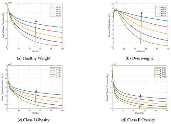
Figure 5. Dynamics of the Healthy Weight, Overweight, Class I Obesity, and Class II Obesity compartments under different fractional orders $\wp \in \{0.6,0.7,0.8,0.9,1.0\}$.

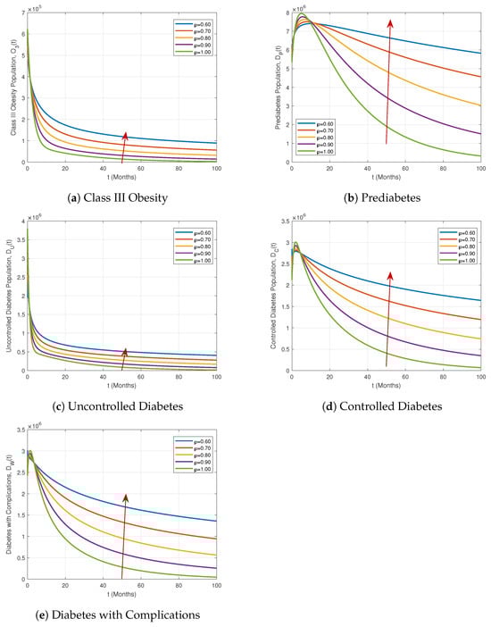
Figure 6. Dynamics of the Class III Obesity, Prediabetes, Uncontrolled Diabetes, Controlled Diabetes, and Diabetes with Complications compartments under different fractional orders $\wp \in \{0.6,0.7,0.8,0.9,1.0\}$.

Similarly, Figure 6 highlights the behavior of the Class III Obesity, Prediabetes, Uncontrolled Diabetes, Controlled Diabetes, and Diabetes with Complications compartments. Notably, the Prediabetes compartment and the Controlled Diabetes and Diabetes with Complications compartments initially rise and then decline over time, exhibiting clear crossover behaviors. These trends become more pronounced as the fractional order deviates from the integer value, demonstrating the model’s sensitivity to ℘ and its ability to capture realistic disease progression patterns.

These results demonstrate that the proposed ABFDM (7) effectively captures both growth and decay dynamics across all compartments. The observed memory-dependent behaviors and crossover patterns provide strong evidence of the model’s suitability for representing real-world epidemiological scenarios and evaluating intervention strategies.

5.2. Impact of Control Strategies

In this subsection, we investigate the effect of treatment interventions as control strategies. Figure 7 and Figure 8 illustrate the influence of varying treatment rates ${\tau }_v\in \{1,4,7,10\}$ and ${\tau }_1\in \{0.9,2.9,4.9,6.9\}$ on the most affected compartments.

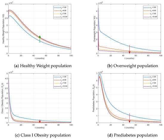
Figure 7. Impact of varying treatment rates ${\tau }_v\in \{1,4,7,10\}$ on key population compartments, with fractional order $\wp =0.96$ and other parameters as in Table 1. Green arrows indicate population increases, and red arrows indicate decreases as the treatment rate for the overweight population rises.

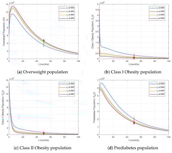
Figure 8. Effects of varying treatment rates ${\tau }_1\in \{0.9,2.9,4.9,6.9\}$ for Obesity Stage I on key population compartments. The fractional order is $\wp =0.96$, with other parameters as in Table 1. Green arrows indicate population increases, and red arrows indicate decreases as the treatment rate rises.

Table 2 demonstrates that increasing the treatment rate ${\tau }_v$ significantly reduces the prevalence of overweight, obesity, and diabetes-related compartments. Specifically, a fourfold increase in treatment lowers uncontrolled diabetes ($D_U$) by 72.68% and diabetes with complications ($D_W$) by 67.52%, while a tenfold increase further decreases prediabetes ($D_P$) by 89.45% and diabetic complications ($D_W$) by 73.17%. As illustrated in Figure 7, higher treatment rates enhance the healthy weight population while simultaneously reducing the overweight, Class I obesity, and prediabetes populations.

Table 2. Percentage (%) impact of treatment rate ${\tau }_v\in \{1,4,7,10\}$ on the population compartments.

Compartment	${\mathit{\tau }}_{\mathit{v}}=1$	${\mathit{\tau }}_{\mathit{v}}=4$	${\mathit{\tau }}_{\mathit{v}}=7$	${\mathit{\tau }}_{\mathit{v}}=10$
V	$-59.83\%$	$-85.89\%$	$-91.45\%$	$-93.86\%$
$O_1$	$-58.66\%$	$-84.00\%$	$-89.39\%$	$-91.74\%$
$O_2$	$-56.70\%$	$-81.00\%$	$-86.16\%$	$-88.40\%$
$O_3$	$-52.01\%$	$-74.11\%$	$-78.79\%$	$-80.83\%$
$D_P$	$-57.86\%$	$-82.10\%$	$-87.23\%$	$-89.45\%$
$D_U$	$-51.72\%$	$-72.68\%$	$-77.08\%$	$-78.98\%$
$D_C$	$-49.29\%$	$-68.39\%$	$-72.35\%$	$-74.06\%$
$D_W$	$-48.54\%$	$-67.52\%$	$-71.47\%$	$-73.17\%$

Table 3 shows that increasing treatment for Class I obesity (${\tau }_1$) markedly reduces obesity and diabetes-related compartments. A moderate increase (${\tau }_1=2.9$) lowers Class I and II obesity by 74.85% and 72.02%, respectively, while more than doubling the overweight population (V) to 102.58%. The highest treatment level (${\tau }_1=6.9$) further decreases Class I and II obesity by 87.65% and 84.31%, respectively, and raises the overweight population to 119.55%. This increase occurs because individuals leaving the Class I obesity compartment initially transition to the overweight compartment at rate ${\tau }_1$ before potentially moving to the healthy weight class at rate ${\tau }_v$. Prediabetes ($D_P$) and uncontrolled diabetes ($D_U$) decline by 36.91% and 32.89%, respectively. As illustrated in Figure 8, intensified Class I obesity interventions shift populations toward healthier compartments, highlighting the stepwise impact of targeted treatment strategies.

Table 3. Percentage (%) impact of treatment rate ${\tau }_1\in \{0.9,2.9,4.9,6.9\}$ on the population compartments.

Compartment	${\mathit{\tau }}_1=0.9$	${\mathit{\tau }}_1=2.9$	${\mathit{\tau }}_1=4.9$	${\mathit{\tau }}_1=6.9$
V	$66.33\%$	$102.58\%$	$113.98\%$	$119.55\%$
$O_1$	$-47.87\%$	$-74.85\%$	$-83.43\%$	$-87.65\%$
$O_2$	$-46.11\%$	$-72.02\%$	$-80.26\%$	$-84.31\%$
$O_3$	$-42.06\%$	$-65.63\%$	$-73.12\%$	$-76.79\%$
$D_P$	$-20.07\%$	$-31.48\%$	$-35.12\%$	$-36.91\%$
$D_U$	$-18.03\%$	$-28.12\%$	$-31.32\%$	$-32.89\%$
$D_C$	$-17.45\%$	$-27.02\%$	$-30.03\%$	$-31.50\%$
$D_W$	$-17.08\%$	$-26.49\%$	$-29.46\%$	$-30.91\%$

Table 4 summarizes the cumulative impact of all treatments on the population compartments. The interventions substantially reduce obesity and diabetes-related populations: Class I, II, and III obesity decrease by 17.11%, 20.25%, and 20.58%, respectively, while prediabetes declines by 12.57%. Uncontrolled, controlled, and complicated diabetes compartments decrease by 4.91%, 2.91%, and 2.69%, respectively. The overweight population (V) is reduced by 8.93%. Figure 9 and Figure 10 confirm these trends, and the bar plot in Figure 10f illustrates the percentage impact of treatments over 100 months. Overall, combined treatment strategies effectively mitigate obesity and diabetes burdens, with the largest reductions in higher obesity classes and prediabetes.

Table 4. Cumulative impact of implementing all the treatments on the model compartments.

Compartment	No Treatment	With Treatment	% Change
$V\left(t\right)$	14,902,175	13,570,988	$-8.93\%$
$O_1\left(t\right)$	4,506,710	3,735,536	$-17.11\%$
$O_2\left(t\right)$	1,151,942	918,661	$-20.25\%$
$O_3\left(t\right)$	314,059	249,425	$-20.58\%$
$D_P\left(t\right)$	14,583,338	12,750,533	$-12.57\%$
$D_U\left(t\right)$	1,114,030	1,059,351	$-4.91\%$
$D_C\left(t\right)$	3,962,116	3,846,893	$-2.91\%$
$D_W\left(t\right)$	3,415,880	3,323,971	$-2.69\%$

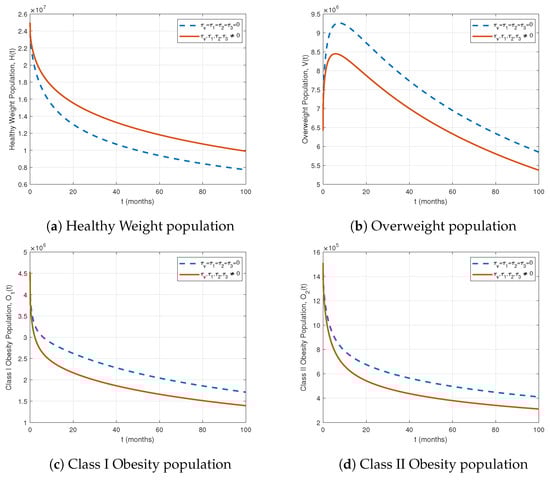
Figure 9. Comparison of population compartments with and without treatment for $\wp =0.65$.

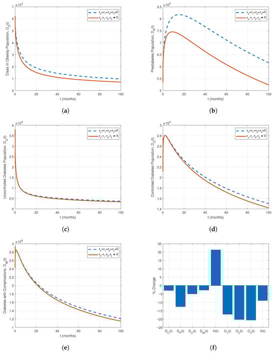
Figure 10. Comparison of population compartments with and without treatment for $\wp =0.65$. (a) Class III Obesity, (b) Prediabetes, (c) Uncontrolled Diabetes, (d) Controlled Diabetes, (e) Diabetes with Complications, (f) Percentage impact of treatments on all compartments.

6. Conclusions and Prospects for Future Work

In this study, we developed and analyzed a fractional-order dynamical model for diabetes progression using the Atangana–Baleanu fractional operator in the Caputo sense with order $\wp \in (0,1)$. Theoretical analyses confirmed the existence, uniqueness, positivity, and boundedness of solutions, and the system’s stability was rigorously established via the Ulam–Hyers $\left(\mathbb{UH}\right)$ stability criterion.

Numerical simulations, informed by initial population data from Saudi Arabia, highlight the substantial impact of targeted Class I obesity treatment (${\tau }_1$) on population compartments. Moderate treatment (${\tau }_1=2.9$) reduces Class I and II obesity by 74.85% and 72.02%, respectively, while increasing the overweight population (V) to 102.58%. The highest treatment level (${\tau }_1=6.9$) further decreases Class I and II obesity by 87.65% and 84.31%, respectively, raising the overweight population to 119.55%. Prediabetes ($D_P$), uncontrolled diabetes ($D_U$), and diabetes with complications ($D_W$) decline by 36.91%, 32.89%, and 30%, respectively. The rise in the overweight population occurs because individuals treated from Class I obesity first transition to the overweight compartment before further treatment moves them to the healthy weight compartment. These results demonstrate that intensified Class I obesity interventions shift populations toward healthier states and effectively mitigate obesity and diabetes progression.

Comparative analyses of scenarios with and without treatment underscore the critical importance of early interventions, particularly in curbing obesity at all stages. Preventing progression from obesity to prediabetes and diabetes is most effective when integrated with public health measures, especially for high-risk populations. Although the current study uses data from Saudi Arabia, the model framework is adaptable to other regions, highlighting its potential to inform global health strategies.

Future work could enhance the model by incorporating a generalized convolution kernel [41] to capture more complex temporal and spatial disease patterns. Additionally, including nonlinear interactions among compartments and dynamic treatment functions would improve predictive accuracy and realism. These refinements would strengthen the model’s utility as a tool for designing optimized diabetes control strategies and guiding evidence-based public health policy.

References

- Sun, H.; Saeedi, P.; Karuranga, S.; Pinkepank, M.; Ogurtsova, K.; Duncan, B.B.; Stein, C.; Basit, A.; Chan, J.C.N.; Mbanya, J.C.; et al. IDF Diabetes Atlas: Global, regional and country-level diabetes prevalence estimates for 2021 and projections for 2045. Diabetes Res. Clin. Pract. 2022, 183, 109119. [Google Scholar] [CrossRef] [PubMed]
- Owens, D.R.; Gurudas, S.; Sivaprasad, S.; Zaidi, F.; Tapp, R.; Kazantzis, D.; Evans, L.; Thomas, R.L. IDF Diabetes Atlas: A worldwide review of studies utilizing retinal photography to screen for diabetic retinopathy from 2017 to 2024 inclusive. Diabetes Res. Clin. Pract. 2025, 226, 112346. [Google Scholar] [CrossRef]
- Huang, X.; Wu, Y.; Ni, H.; Xu, H.; He, Y. Global, regional, and national burden of type 2 diabetes mellitus caused by high BMI from 1990 to 2021, and forecasts to 2045: Analysis from the global burden of disease study 2021. Front. Public Health 2025, 13, 1515797. [Google Scholar] [CrossRef]
- Taylor, R. Understanding the cause of type 2 diabetes. Lancet Diabetes Endocrinol. 2024, 12, 664–673. [Google Scholar] [CrossRef]
- Chandrasekaran, P.; Weiskirchen, R. The role of obesity in type 2 diabetes mellitus—An overview. Int. J. Mol. Sci. 2024, 25, 1882. [Google Scholar] [CrossRef] [PubMed]
- Jajarmi, A.; Ghanbari, B.; Baleanu, D. A new and efficient numerical method for the fractional modeling and optimal control of diabetes and tuberculosis co-existence. Chaos 2019, 29, 093111. [Google Scholar] [CrossRef]
- Kouidere, A.; Labzai, A.; Ferjouchia, H.; Balatif, O.; Rachik, M. A New Mathematical Modeling with Optimal Control Strategy for the Dynamics of Population of Diabetics and Its Complications with Effect of Behavioral Factors. J. Appl. Math. 2020, 2020, 1943410. [Google Scholar] [CrossRef]
- Delgado Moya, E.M.; Rodriguez, R.A.; Pietrus, A.; Bernard, S. A study of fractional optimal control of overweight and obesity in a community and its impact on the diagnosis of diabetes. Math. Model. Numer. Simul. Appl. 2024, 4, 514–543. [Google Scholar] [CrossRef]
- Omame, A.; Nwajeri, U.K.; Abbas, M.; Onyenegecha, C.P. A fractional order control model for Diabetes and COVID-19 co-dynamics with Mittag-Leffler function. Alex. Eng. J. 2022, 61, 7619–7635. [Google Scholar] [CrossRef]
- Mollah, S.; Biswas, S. Optimal control for the complication of Type 2 diabetes: The role of awareness programs by media and treatment. Int. J. Dyn. Control 2022, 11, 877–891. [Google Scholar] [CrossRef] [PubMed]
- Youssef, M.I.; Maina, R.M.; Gathungu, D.K.; Radwan, A. A Qualitative Analysis and Discussion of a New Model for Optimizing Obesity and Associated Comorbidities. Symmetry 2025, 17, 1216. [Google Scholar] [CrossRef]
- Dubey, R.S.; Goswami, P. Mathematical model of diabetes and its complication involving fractional operator without singular kernel. Discret. Contin. Dyn. Syst. Ser. S 2021, 14, 2151–2161. [Google Scholar] [CrossRef]
- Yadav, P.; Jahan, S.; Shah, K.; Peter, O.J.; Abdeljawad, T. Fractional-order modelling and analysis of diabetes mellitus: Utilizing the Atangana–Baleanu–Caputo (ABC) operator. Alex. Eng. J. 2023, 81, 200–209. [Google Scholar] [CrossRef]
- Khan, H.; Alzabut, J.; Almutairi, D.K.; Alqurashi, W.K. The use of artificial intelligence in data analysis with error recognitions in liver transplantation in HIV-AIDS patients using modified ABC fractional order operators. Fractal Fract. 2024, 9, 16. [Google Scholar] [CrossRef]
- Nisar, K.S.; Ahmad, A.; Farman, M.; Hincal, E.; Zehra, A. Modeling and mathematical analysis of fractional order Eye infection (conjunctivitis) virus model with treatment impact: Prelicence and dynamical transmission. Alex. Eng. J. 2024, 107, 33–46. [Google Scholar] [CrossRef]
- Adom-Konadu, A.; Bonyah, E.; Sackitey, A.L.; Anokye, M.; Asamoah, J.K.K. A fractional order Monkeypox model with protected travelers using the fixed point theorem and Newton polynomial interpolation. Healthc. Anal. 2023, 3, 100191. [Google Scholar] [CrossRef]
- Dasumani, M.; Lassong, B.S.; Akgül, A.; Osman, S.; Moore, S.E. Analyzing the dynamics of human papillomavirus transmission via fractal and fractional dimensions under Mittag-Leffler Law. Model. Earth Syst. Environ. 2024, 10, 7225–7249. [Google Scholar] [CrossRef]
- Podlubny, I. Fractional Differential Equations: An Introduction to Fractional Derivatives, Fractional Differential Equations, to Methods of Their Solution and Some of Their Applications; Elsevier: Amsterdam, The Netherlands, 1998; Volume 198. [Google Scholar]
- Atangana, A.; Baleanu, D. New fractional derivatives with non-local and non-singular kernel: Theory and application to heat transfer model. Therm. Sci. 2016, 20, 763–769. [Google Scholar] [CrossRef]
- Kumar, S.; Chauhan, R.P.; Aly, A.A.; Momani, S.; Hadid, S. A study on fractional HBV model through singular and non-singular derivatives. Eur. Phys. J. Spec. Top. 2022, 231, 1885–1904. [Google Scholar] [CrossRef] [PubMed]
- Lassong, B.S.; Dasumani, M.; Mung’atu, J.K.; Moore, S.E. Power and Mittag–Leffler laws for examining the dynamics of fractional unemployment model: A comparative analysis. Chaos Solitons Fractals X 2024, 13, 100117. [Google Scholar] [CrossRef]
- Mursaleen, M.; Ansari, K.J. On the stability of some positive linear operators from approximation theory. Bull. Math. Sci. 2015, 5, 147–157. [Google Scholar] [CrossRef]
- Centers for Disease Control and Prevention (CDC). About Adult BMI; U.S. Department of Health & Human Services: Washington, DC, USA, 2024. Available online: https://www.cdc.gov/bmi/adult-calculator/bmi-categories.html (accessed on 10 October 2025).
- Alshammari, F.S. A mathematical model to investigate the transmission of COVID-19 in the Kingdom of Saudi Arabia. Comput. Math. Methods Med. 2020, 2020, 9136157. [Google Scholar] [CrossRef] [PubMed]
- Moya, E.D.; Pietrus, A.; Bernard, S. Mathematical model for the study of obesity in a population and its impact on the growth of diabetes. Math. Model. Anal. 2023, 28, 611–635. [Google Scholar] [CrossRef]
- Guh, D.P.; Zhang, W.; Bansback, N.; Amarsi, Z.; Birmingham, C.L.; Anis, A.H. The incidence of co-morbidities related to obesity and overweight: A systematic review and meta-analysis. BMC Public Health 2009, 9, 88. [Google Scholar] [CrossRef] [PubMed]
- Apovian, C.M.; Aronne, L.J.; Barenbaum, S. Obesity-Related Comorbidities. Healio. 24 July 2024. Available online: https://www.healio.com/clinical-guidance/obesity/obesity-related-comorbidities (accessed on 10 October 2025).
- Lartey, S.T.; Si, L.; Otahal, P.; de Graaff, B.; Boateng, G.O.; Biritwum, R.B.; Minicuci, N.; Kowal, P.; Magnussen, C.G.; Palmer, A.J. Annual transition probabilities of overweight and obesity in older adults: Evidence from World Health Organization Study on global AGEing and adult health. Soc. Sci. Med. 2020, 247, 112821. [Google Scholar] [CrossRef]
- Navarro-Pérez, J.; Orozco-Beltran, D.; Gil-Guillen, V.; Pallares, V.; Valls, F.; Fernandez, A.; Perez-Navarro, A.M.; Sanchis, C.; Dominguez-Lucas, A.; Martin-Moreno, J.M.; et al. Mortality and cardiovascular disease burden of uncontrolled diabetes in a registry-based cohort: The ESCARVAL-risk study. BMC Cardiovasc. Disord. 2018, 18, 180. [Google Scholar] [CrossRef]
- Ahmad, S.; Kirane, M. On a fractional-order mathematical model to assess the impact of diabetes and its associated complications in the United Arab Emirates. Math. Methods Appl. Sci. 2024, 47, 6892–6902. [Google Scholar] [CrossRef]
- Weiner, A.; Zhang, M.; Ren, S.; Tchang, B.; Gandica, R.; Murillo, J. Progression from prediabetes to type 2 diabetes mellitus in adolescents: A real world experience. Front. Clin. Diabetes Healthc. 2023, 4, 1181729. [Google Scholar] [CrossRef]
- Tuso, P. Prediabetes and lifestyle modification: Time to prevent a preventable disease. Perm. J. 2014, 18, 88–93. [Google Scholar] [CrossRef]
- World Health Organisation. Diabetes; WHO: Geneva, Switzerland, 2024; Available online: https://www.who.int/news-room/fact-sheets/detail/diabetes (accessed on 10 October 2025).
- Yamaguchi, S.; Waki, K.; Tomizawa, N.; Waki, H.; Nannya, Y.; Nangaku, M.; Kadowaki, T.; Ohe, K. Previous dropout from diabetic care as a predictor of patients’ willingness to use mobile applications for self-management: A cross-sectional study. J. Diabetes Investig. 2017, 8, 542–549. [Google Scholar] [CrossRef]
- Karter, A.J.; Nundy, S.; Parker, M.M.; Moffet, H.H.; Huang, E.S. Incidence of remission in adults with type 2 diabetes: The Diabetes & Aging Study. Diabetes Care 2014, 37, 3188–3195. [Google Scholar] [CrossRef] [PubMed]
- Rapoport, M.; Chetrit, A.; Cantrell, D.; Novikov, I.; Roth, J.; Dankner, R. Years of potential life lost in pre-diabetes and diabetes mellitus: Data from a 40-year follow-up of the Israel study on Glucose intolerance, Obesity and Hypertension. BMJ Open Diabetes Res. Care 2021, 9, e001981. [Google Scholar] [CrossRef] [PubMed]
- Ye, H.; Gao, J.; Ding, Y. A generalized Gronwall inequality and its application to a fractional differential equation. J. Math. Anal. Appl. 2007, 328, 1075–1081. [Google Scholar] [CrossRef]
- Khan, H.; Alzabut, J.; Gómez-Aguilar, J.F.; Alkhazan, A. Essential criteria for existence of solution of a modified-ABC fractional order smoking model. Ain Shams Eng. J. 2024, 15, 102646. [Google Scholar] [CrossRef]
- Khan, H.; Alzabut, J.; Almutairi, D.K.; Alqurashi, W.K.; Pinelas, S.; Tunç, O.; Azim, M.A. A coupled nonlinear system of integro-differential equations using modified ABC operator. Fractals 2025, 33, 2540105. [Google Scholar] [CrossRef]
- International Diabetes Federation. Saudi Arabia. 2024. Available online: https://idf.org/our-network/regions-and-members/middle-east-and-north-africa/members/saudi-arabia/ (accessed on 30 October 2025).
- Youssef, M.I.; Abdou, M.A.; Gharbi, A. An Iterative Approximate Method for Solving 2D Weakly Singular Fredholm Integral Equations of the Second Kind. Mathematics 2025, 13, 1854. [Google Scholar] [CrossRef]
Disclaimer/Publisher’s Note: The statements, opinions and data contained in all publications are solely those of the individual author(s) and contributor(s) and not of MDPI and/or the editor(s). MDPI and/or the editor(s) disclaim responsibility for any injury to people or property resulting from any ideas, methods, instructions or products referred to in the content. |
© 2025 by the authors. Licensee MDPI, Basel, Switzerland. This article is an open access article distributed under the terms and conditions of the Creative Commons Attribution (CC BY) license (https://creativecommons.org/licenses/by/4.0/).