Article

Multifractality Between PM2.5, Air Quality Index and Ozone for Sites of California

by
Werner Kristjanpoller
1,* and
Marcel C. Minutolo
2
1
Departamento de Industrias, Universidad Tecnica Federico Santa Maria, Valparaíso 2390123, Chile
2
Rockwell School of Business, Robert Morris University, Moon Township, PA 15108, USA
*
Author to whom correspondence should be addressed.
Fractal Fract. 2025, 9(12), 821; https://doi.org/10.3390/fractalfract9120821
Submission received: 5 November 2025 / Revised: 11 December 2025 / Accepted: 12 December 2025 / Published: 16 December 2025

Abstract

Understanding the temporal dynamics of urban air pollution is essential for effective environmental management, yet the nonlinear and scale-dependent behavior of key pollutants remains insufficiently explored. This study examines the multifractal properties of fine particulate matter ( P M 2.5 ), ozone ( O 3 ), and the Air Quality Index (AQI) across four major urban locations in California—Los Angeles, Orange, Riverside–Rubidoux, and Riverside–Mira Loma—regions characterized by persistent air-quality challenges and high population exposure. Using Multifractal Detrended Fluctuation Analysis (MF-DFA), we assess long-range dependence, heterogeneity, and cross-pollutant interactions to address the central question of whether these pollutants exhibit genuine multifractal behavior and how it varies across locations. The results reveal strong multifractality in all series, with spectrum widths ranging from 0.42 to 0.71 for P M 2.5 -AQI and from 0.28 to 0.46 for O 3 -AQI, indicating pronounced scale-dependent variability. Los Angeles consistently exhibited the widest spectra, reflecting greater temporal complexity. The generalized Hurst exponent at q = 2 remained between 0.52 and 0.58 across all pollutant pairs, indicating persistent dynamics. Surrogate-data testing further confirmed that 60–75% of the observed multifractality arises from intrinsic long-range correlations rather than distributional effects. Overall, this study demonstrates that urban air pollutants in California display rich multifractal structures that differ systematically across regions, reflecting local emission patterns and atmospheric processes. These findings highlight the relevance of multifractal analysis as a powerful tool for improving air-quality modeling, forecasting, and policy design in densely populated environments.

1. Introduction

Human-induced impacts on the environment are undeniable [1]. Rapid urbanization and industrialization have led to a substantial increase in airborne particulate matter, contributing to elevated ozone levels and deteriorating air quality [2,3]. Consequently, urban environments face a critical challenge from air pollution-particularly particulate matter ( P M 2.5 ), ozone ( O 3 ), and the resulting elevated Air Quality Index (AQI) [4,5]. These pollutants have profound and multifaceted effects on human health, urban ecosystems, and overall quality of life in cities [6,7].
From a public health perspective, P M 2.5 can penetrate the respiratory system deep and even enter the bloodstream, leading to a wide range of serious diseases, including asthma, chronic obstructive pulmonary disease, cardiovascular disorders, and premature mortality [8]. Furthermore, ground-level ozone, a major component of smog, causes respiratory irritation, exacerbates asthma, and damages lung tissue [9].
Air pollution also undermines urban environmental quality by reducing visibility, harming vegetation, and degrading urban aesthetics [10,11]. It adversely affects urban green spaces, contributes to the urban heat island effect, and can disrupt social and economic activity [12,13]. Elevated AQI levels often force schools and businesses to close and restrict outdoor activities [14,15]. The significant health and environmental burdens associated with these pollutants therefore demand urgent mitigation measures. Reducing emissions from transportation, industrial processes, and residential sources is vital to improving air quality. Similarly, implementing effective monitoring systems and adopting sound urban planning strategies are essential to mitigate the impacts of P M 2.5 , O 3 , and high AQI levels.
However, as highlighted in previous research (e.g., [16,17,18]), the relationships between P M 2.5 , O 3 and AQI exhibit multifractal characteristics, making them complex and difficult to predict. This inherent complexity poses significant challenges for policy makers seeking to design and implement efficient interventions that improve urban air quality while promoting economic growth and improving the livability of urban areas.
Given the intrinsic properties of environmental time series-autocorrelation, heteroscedasticity, and nonlinearity-this study applies Rescaled Range (R/S) Analysis [19,20] to determine the fractal dimension of the data. R/S analysis allows for the detection of long-term persistence and dependence in non-periodic and non-stationary series, even when data extend beyond the analyzed time window. This method is particularly suitable for identifying long-term correlations in stochastic processes.
Fractal analysis has evolved significantly and has been adapted for diverse applications. Peng et al. [21] introduced the Fluctuation Analysis (FA) method, which was later refined through the Detrended Fluctuation Analysis (DFA) technique [22]. To overcome the limitations of monofractal models, Multifractal Detrended Fluctuation Analysis (MF-DFA) was developed [23,24], enabling the characterization of multiple scaling behaviors within a single time series. Recognizing that many signals exhibit asymmetric dynamics, Álvarez-Ramírez et al. [25] proposed the Asymmetric DFA (A-DFA), which was later extended by Cao et al. [26] into the Asymmetric Multifractal DFA (A-MFDFA) framework. Zhang et al. [16] further enhanced this methodology by introducing the Asymmetric Multifractal Detrending Moving Average (A-MFDMA) approach to analyze P M 2.5 concentrations, improving upon previous techniques in performance and robustness.
Multifractal modeling has proven valuable in a wide range of fields, including DNA analysis [27], meteorology [28,29,30,31], cardiac dynamics [32,33,34], fire dynamics [35], electrical conductivity [36], image recognition [37,38], rare earth element analysis [39], network traffic [40,41], materials science [42], earthquake dynamics [43], and hydrology [44], among many others. Given its proven ability to capture persistence, nonlinearity, and long-range dependence, the multifractal approach has gained widespread acceptance. Its growing application to environmental and atmospheric data [16,17,18,45,46,47] underscores its potential for advancing our understanding of air pollution dynamics.
The present study builds on previous work employing fractal-based techniques by extending the analysis to additional air quality indicators within a North American context. By incorporating fractal analysis—including AQI as a key variable—the research provides deeper insights into the nonlinear and scale-dependent interactions among air pollution, human health, and the urban environment, with the ultimate goal of informing more effective air quality management and public health policies that enhance environmental resilience and urban livability. The remainder of the manuscript is organized as follows: Section 2 presents the data and methodology, Section 3 reports the empirical results, Section 4 discusses the findings, and Section 5 concludes with key insights and policy implications.

2. Materials and Methods

2.1. Data

Four locations in the state of California were selected for this analysis based on the availability and continuity of air quality data provided by the United States Environmental Protection Agency (EPA) (https://www.epa.gov/outdoor-air-quality-data accessed on 4 November 2025). The selected monitoring stations were:
  • Los Angeles—North Main Street (NMS)
  • Orange—Anaheim (A)
  • Riverside—Rubidoux (R)
  • Riverside—Mira Loma, Van Buren (ML)
For each location, daily time series data for particulate matter ( P M 2.5 ), ozone ( O 3 ), and the Air Quality Index (AQI) were collected from 1 January 2021, to 31 August 2024, yielding a total of 1339 observations per series (County code and site numbers: NMS-37,1103; A-59,7; R-65,8001; ML-65,8005). EPA computes daily pollutant concentrations using 24 h averages from midnight to midnight. A daily value is considered valid only when at least 18 of the 24 hourly measurements are available.
Among the four sites, Mira Loma and Rubidoux, both located in Riverside County, recorded the highest average P M 2.5 concentrations during the study period and exhibited the greatest P M 2.5 volatility (see Table 1). Similarly, Mira Loma presented the worst average AQI ( P M 2.5 ) values, followed by Los Angeles-North Main Street. Regarding ozone, the pattern was comparable, with Mira Loma and Rubidoux again showing the highest mean levels. In all three locations—Los Angeles (NMS), Mira Loma, and Rubidoux—the maximum AQI values for both P M 2.5 and O 3 reached the “unhealthy” category, according to EPA air quality standards.

2.2. Methodology

The Multi-Fractal Detrended Fluctuation Analysis (MFDFA) is a method used to investigate the asymmetric multifractal characteristics of time series. This technique was first introduced by Peng et al. [21] as Detrended Fluctuation Analysis (DFA) and later generalized to MFDFA by Kantelhardt et al. [48]. The MFDFA method is particularly effective for analyzing highly non-stationary time series and consists of five steps.
Given time series x i and y i with observations N, the MFDFA process can be summarized as follows.
1. Construct the profile:
X ( i ) = t = 1 i ( x t x ¯ ) , i = 1 , , N
Y ( i ) = t = 1 i ( y t y ¯ ) , i = 1 , , N
Here, x ¯ and y ¯ represent the average of the time series x i and y i , respectively.
2. Divide the profiles X ( i ) and Y ( i ) into N s = [ N / s ] nonoverlapping windows of equal length s. Note that since the total length N is not necessarily a multiple of the time scale s, some segments of the profile may be left unprocessed at the end of the series. This procedure is also applied from the end of the series, resulting in 2 N s segments.
3. For each of the 2 N s segments, estimate the trend X v ( i ) and Y v ( i ) using linear regression:
X v ( i ) = a X v + b X v · i
Y v ( i ) = a Y v + b Y v · i
The detrended covariance for each segment is then calculated as follows:
F ( v , s ) = 1 s i = 1 s [ X [ ( v 1 ) s + i ] X v ( i ) ] [ Y [ ( v 1 ) s + i ] Y v ( i ) ]
for each segment v, v = 1 , , N s , and
F ( v , s ) = 1 s i = 1 s [ X [ N ( v N s ) s + i ] X v ( i ) ] [ Y [ N ( v N s ) s + i ] Y v ( i ) ]
for each segment v, v = N s + 1 , , 2 N s .
4. Average all segments to obtain the qth order fluctuation function. This captures the different behaviors of trends in the time series x t :
F q + ( s ) = 1 M + v = 1 2 N s s i g n ( b X v ) + 1 2 [ F ( v , s ) ] q / 2 1 / q
F q ( s ) = 1 M v = 1 2 N s [ s i g n ( b X v ) 1 ] 2 [ F ( v , s ) ] q / 2 1 / q
for q 0 . When q = 0 :
F 0 + ( s ) = exp 1 2 M + v = 1 2 N s s i g n ( b X v ) + 1 2 [ F ( v , s ) ]
F 0 ( s ) = exp 1 2 M v = 1 2 N s [ s i g n ( b X v ) 1 ] 2 [ F ( v , s ) ]
where M + = v = 1 2 N s s i g n ( b X v ) + 1 2 and M = v = 1 2 N s [ s i g n ( b X v ) 1 ] 2 represent the number of sub-time series with positive and negative trends, respectively. We assume b X v 0 for all v = 1 , , 2 N s , ensuring M + + M = 2 N s .
The traditional MF-DFA is implemented by calculating the average fluctuation function for q 0 :
F q ( s ) = 1 2 N s v = 1 2 N s [ F ( v , s ) ] q / 2 1 / q
For q = 0 :
F q ( s ) = exp 1 4 N s v = 1 2 N s ln [ F ( v , s ) ]
The parameter q functions as a selective filter that adjusts the influence of intra-box variances and covariances. When q takes large positive values, the contribution to the sums in Equations (11) and (12) are dominated by the segments (of size s) exhibiting the strongest fluctuations. Conversely, for sufficiently negative q, the segments with the smallest fluctuations exert the greatest influence.
5. Generalized Hurst exponent determination The traditional MFDFA is implemented by computing the average fluctuation function for q 0 :
F q ( s ) = 1 2 N s v = 1 2 N s [ F ( v , s ) ] q / 2 1 / q
For q = 0 , it is calculated as:
F q ( s ) = exp 1 4 N s v = 1 2 N s ln [ F ( v , s ) ]
If multifractal cross-correlation is present, the fluctuation function F q ( s ) should follow a power–law relationship as Equation (15).
F q ( s ) s λ ( q )
where λ ( q ) is a scaling exponent that quantitatively captures the fractal properties of the cross-correlations. In the case of monofractal cross-correlation, λ ( q ) remains constant and does not vary with q. Therefore, any systematic dependence of λ ( q ) on q provides clear evidence of multifractality in the cross-correlations under investigation. F q ( s ) characterizes the scaling behavior according to Equation (16), capturing how its fluctuations evolve across different scales, determinating the Generalizaed Hurst exponent Hxy.
F q ( s ) characterizes the scaling behavior according to Equation (16), capturing how fluctuations evolve across different scales and allowing the determination of the generalized Hurst exponent H x y ( q ) . This measure provides insight into whether the underlying dynamics follow a monofractal pattern or exhibit more complex multifractal properties.
F q ( s ) s H x y ( q )
The scaling exponent H x y ( q ) represents the slope of the log-log plot of F q ( s ) versus s, calculated using the ordinary least squares (OLS) method. For q = 2 , H x y ( q ) shares similar properties and interpretations with the Hurst exponent. Specifically,
  • If H x y ( 2 ) > 0.5 , the series exhibits persistence, meaning a positive (negative) change in one measure is statistically more likely to be followed by a positive (negative) change in the other.
  • If H x y ( 2 ) < 0.5 , the series is antipersistent, indicating that a positive (negative) change in one measure is more likely to be followed by a negative (positive) change in the other.
  • If H x y ( 2 ) = 0.5 , the series displays short-range or no auto-correlations, consistent with the behavior of a random walk.
When the scaling exponent H x ( q ) varies with q, the auto-correlation structure is multifractal. For q > 0 , H x ( q ) , H x + ( q ) , and H x ( q ) describe the scaling behavior of large fluctuations, while for q < 0 , they characterize the scaling behavior of small fluctuations.
6. Multifractal spectrum determination The corresponding singularity spectrum f ( α ) is then obtained using the relations given in Equations (17) and (18).
τ ( q ) = q H x y ( q ) 1
f ( α ) = q α τ ( q ) = q [ α H x y ( q ) ] + 1
where τ ( q ) is the multifractal scalling exponent or mass exponenet function, α is the singularity (or Hölder) exponent and f ( α ) denotes the corresponding singularity spectrum, often referred to as the multifractal spectrum. This special case, when applied to a single time series, corresponds to the well-known Multifractal Detrended Fluctuation Analysis (MFDFA). For time series generated by mathematical cascade models, the singularity spectrum f ( α ) associated with the moments of order q range exhibits the form of a symmetric, uppermost segment of an inverted parabola.

Cross-Correlation Test

To evaluate the presence of cross-correlations between the analyzed variables, we employed the cross-correlation test introduced by Podobnik et al. [49]. This procedure allows for a formal assessment of whether statistically significant cross-dependencies exist among the selected pollutant series and the air-quality indicators. The test relies on the Q c c statistic, defined in Equations (19) and (20), which under the null hypothesis of no cross-correlation follows a χ 2 distribution with m degrees of freedom. This framework enables a rigorous examination of the temporal co-movement between P M 2.5 , O 3 , and AQI across the studied monitoring sites.
Q c c ( m ) = N 2 i = 1 m X Y i 2 N i
where
X Y i = k = i + 1 N X t Y t i t = 1 N X t t = 1 N Y t
Figure 1 presents a schematic summary of the methodological framework applied in this study, outlining the sequential steps followed to obtain the results and conduct the corresponding analyses.

3. Results

The analysis was conducted for three variable pairs: P M 2.5 -AQI, O 3 -AQI, and P M 2.5 - O 3 . The AQI values for each site were obtained according to the United States Environmental Protection Agency’s (EPA) standardized tabulation (https://www.airnow.gov/aqi/aqi-basics/ accessed on 4 November 2025) (see Figure A1), which provides distinct indices for P M 2.5 and O 3 concentrations.
Figure 2 depicts the temporal evolution of P M 2.5 concentrations and AQI values across the four study locations. A clear synchronization between the peaks and troughs of P M 2.5 and AQI is evident in all sites, indicating a strong relationship between these variables. This close alignment is expected, as P M 2.5 constitutes a primary determinant in AQI computation. The estimated correlation coefficient between P M 2.5 and AQI for the four locations is approximately 0.95, confirming their strong statistical association.
Figure 3 presents the time evolution of O 3 levels and AQI. Although some correspondence between extreme O 3 and AQI values can be observed, the overall temporal alignment is less consistent compared to that of P M 2.5 . Despite the AQI for O 3 being computed through a similar methodology, the average correlation coefficient between O 3 and AQI is considerably lower—around 0.76. This result suggests that AQI variability is influenced by additional pollutants and meteorological conditions beyond O 3 concentrations alone.
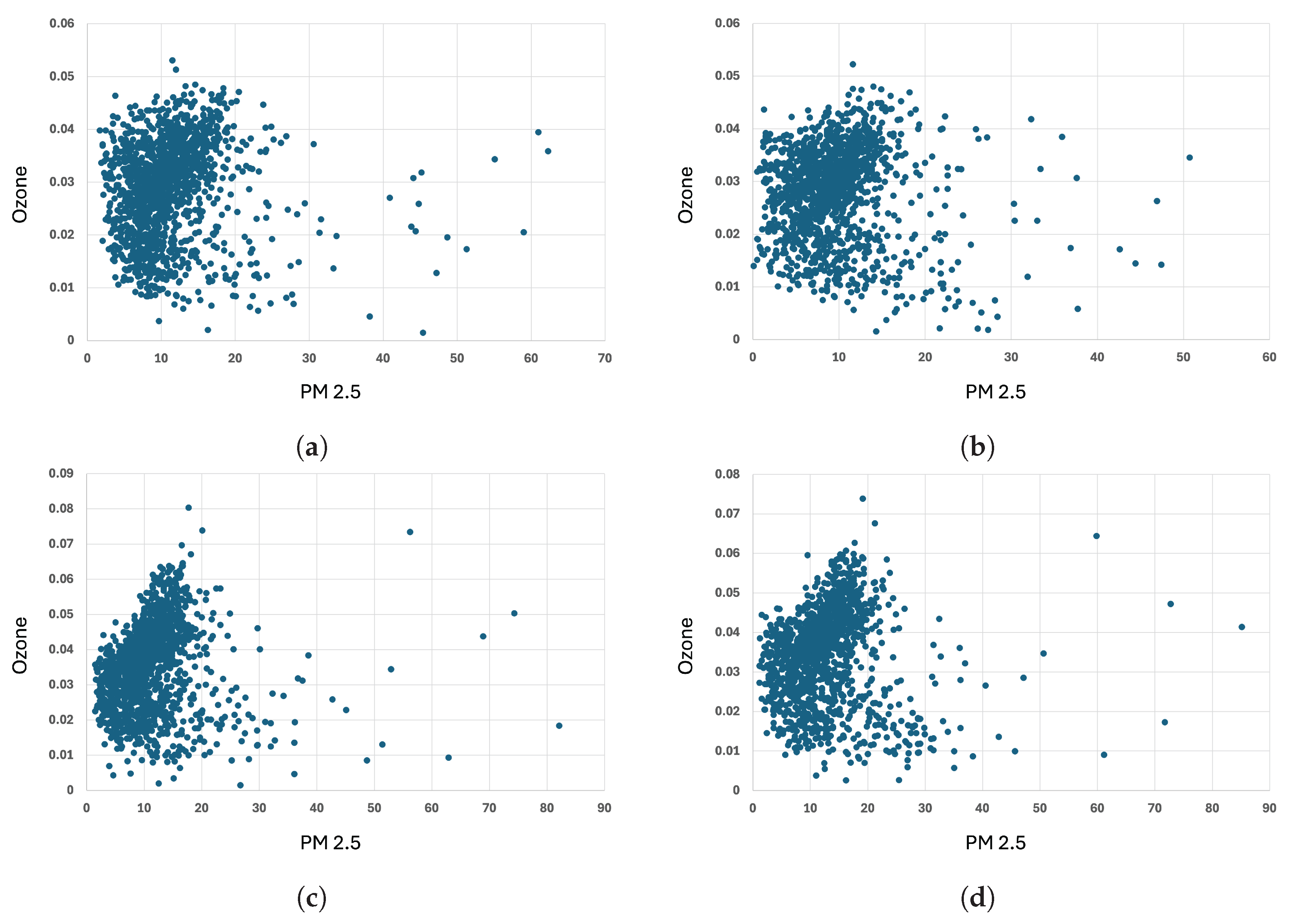
Finally, Figure 4 presents the scatter plots of daily P M 2.5 concentrations and O 3 levels for each monitoring site throughout the study period, seeking to identify potential day-to-day relationships between the two pollutants. Unlike the previous variable pairs, no discernible pattern or functional relationship emerges across the locations. The corresponding correlation coefficients remain close to zero, confirming that fluctuations in P M 2.5 and O 3 occur largely independently.
This absence of co-movement highlights the distinct atmospheric processes influencing each pollutant. While P M 2.5 is dominated by combustion sources, secondary aerosol formation, and local emissions, O 3 is driven primarily by photochemical reactions involving precursors such as NOx and VOCs. The weak coupling observed in the scatter plots suggests that these pollutants respond to different physical, chemical, and meteorological conditions across the analyzed regions. Consequently, understanding their joint behavior requires a multifactorial approach rather than relying on simple linear associations.
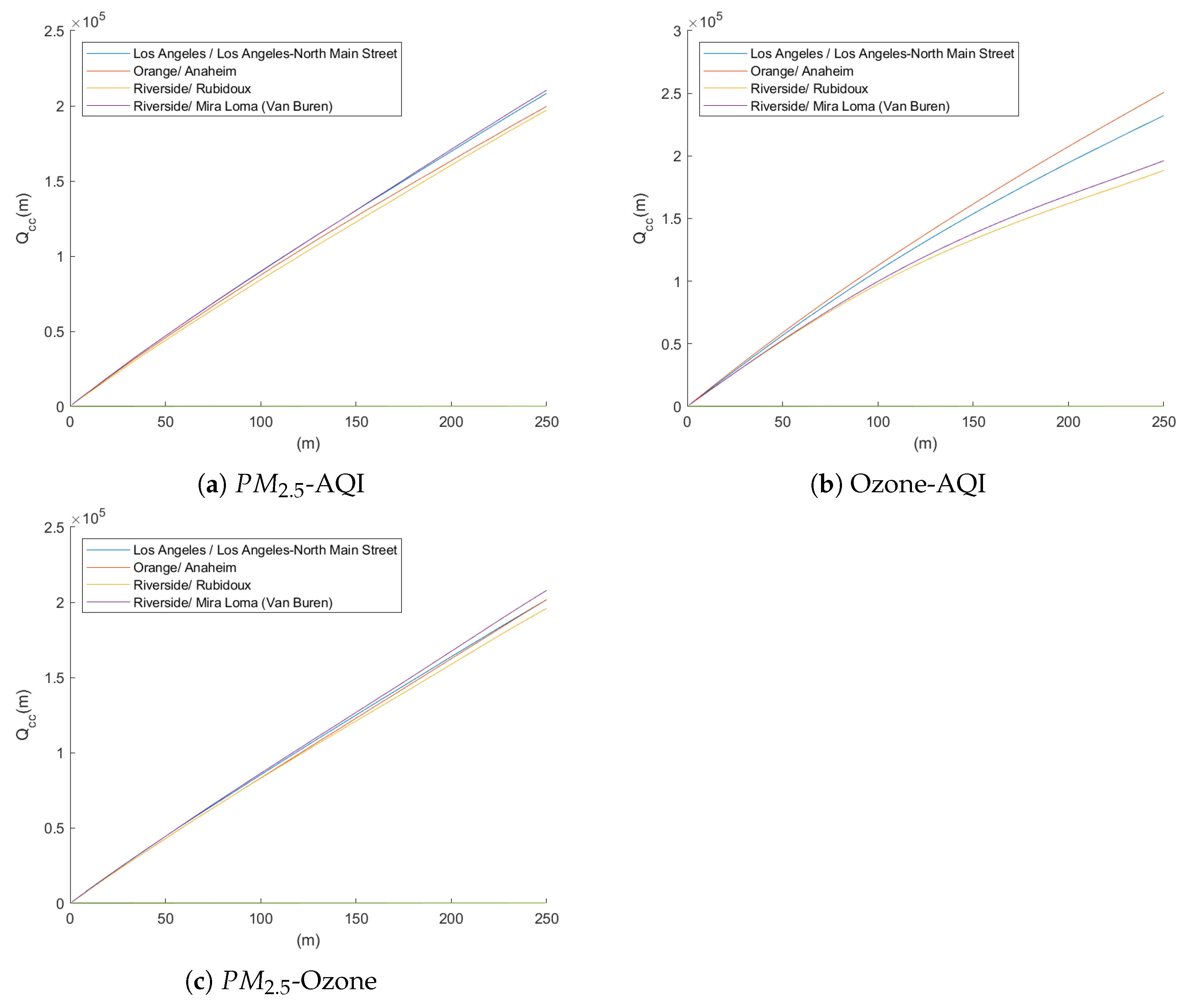
To examine the existence of cross-correlations between the analyzed variables, we applied the cross-correlation test proposed by Podobnik et al. [49]. Our primary objective was to assess whether statistically significant cross-correlations exist among the selected pollutant and air quality indicators.
The results of the cross-correlation test are presented in Figure 5. For all four study locations, significant cross-correlations were identified among the three variable pairs: P M 2.5 -AQI, O 3 -AQI, and P M 2.5 - O 3 . In each case, the critical value lies near the x-axis due to the high magnitudes of the Q c c statistics, confirming the presence of cross-dependence between the time series. This preliminary finding indicates that the analyzed data likely exhibit multifractal characteristics, warranting a more detailed investigation through multifractal detrended analysis in subsequent sections.
The generalized Hurst exponent ( H x y ( q ) ) for the P M 2.5 -AQI relationship (Figure 6a) displays a monotonically decreasing profile across all monitoring sites, indicating that higher-order fluctuations intensify antipersistent behavior. Despite this decline, the overall dynamics remain persistent for most of the q-range at all locations. Among the four sites, Orange/Anaheim exhibits the strongest multifractality, as reflected in a wider spread of H x y ( q ) , while Riverside/Mira Loma shows the weakest multifractality. Additionally, for large positive moments ( q > 4 ), Los Angeles/North Main Street and Riverside/Rubidoux transition toward clear antipersistence, suggesting that extreme fluctuations in these locations tend to reverse rather than reinforce their previous direction.
For the O 3 -AQI pair (Figure 6b), all stations exhibit persistent dynamics combined with a decreasing trend in H x y ( q ) , consistent with multifractal behavior. A notable exception is Orange/Anaheim, where the curve remains nearly flat across all q values, indicating quasi-monofractal behavior. Los Angeles/North Main Street, Riverside/Rubidoux, and Riverside/Mira Loma follow similar patterns for small fluctuations ( q < 3 ). However, for larger fluctuations ( q > 3 ), Los Angeles/North Main Street shows a pronounced drop in persistence, suggesting heightened sensitivity to extreme ozone variations.
For the P M 2.5 - O 3 relationship (Figure 6c), Los Angeles/North Main Street again stands out with the strongest multifractal signature, reflecting complex co-fluctuation structures between the two pollutants. In contrast, Orange/Anaheim, Riverside/Rubidoux, and Riverside/Mira Loma show nearly monofractal behavior for q < 0 , indicating that small fluctuations are relatively uniform and scale-independent. For positive moments ( q > 0 ), Riverside/Rubidoux and Riverside/Mira Loma exhibit a mild reduction in persistence, while Orange/Anaheim shows a more substantial decline, suggesting that larger joint fluctuations between P M 2.5 and O 3 behave differently across these sites.
When examining the Hurst exponent H x y ( 2 ) with its corresponding 95% confidence intervals (Figure 7), all pollutant–indicator pairs across all monitoring sites exhibited values below 0.6, consistently indicating persistent cross-correlation dynamics. Importantly, the confidence intervals largely overlapped across both pollutant pairs and locations, suggesting no statistically significant differences in persistence among the examined relationships. Overall, these findings confirm that all analyzed variable pairs display a persistent Hurst exponent, reinforcing the presence of long-range dependence in their joint fluctuations.
When examining the multifractal spectra of the P M 2.5 –AQI series (Figure 8a), all locations exhibit spectra skewed toward higher α values, indicating persistent dynamics and long-range correlations. Across the four sites, Los Angeles/North Main Street shows the largest spectrum width, reflecting a higher degree of multifractality and suggesting more heterogeneous fluctuation structures in its particulate matter dynamics.
In contrast, the O 3 –AQI spectra (Figure 8b) are also centered at high α values—again signaling persistence—but display substantially narrower spectrum widths relative to the P M 2.5 –AQI case. This narrowing reflects a weaker multifractal signature, implying that ozone concentrations were governed by more homogeneous temporal patterns over the study period. Additionally, the spectrum width is remarkably similar across all locations, indicating that ozone dynamics exhibit comparable multifractal properties in each site.
Finally, the joint P M 2.5 O 3 spectra (Figure 8c) also cluster around high α values and resemble the shape observed for O 3 –AQI, again pointing to persistent cross-fluctuation behavior. As in the previous cases, Los Angeles/North Main Street presents the widest spectrum, consistent with its more complex temporal dependence structure in both pollutants.
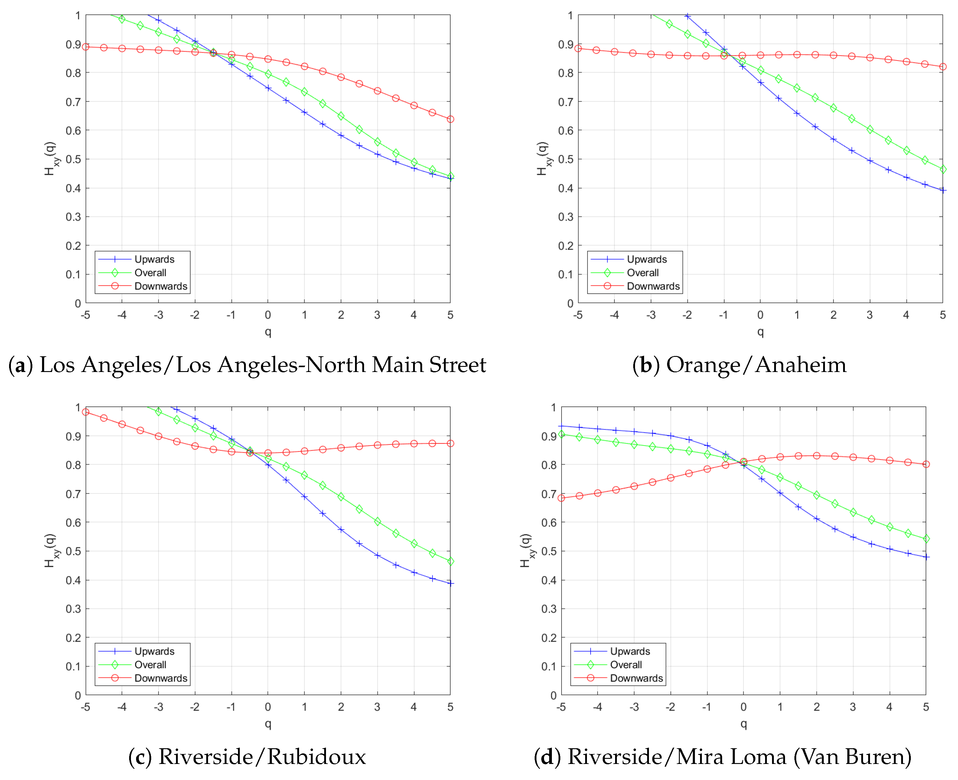
When analyzing the generalized Hurst exponent for the P M 2.5 -AQI pair (Figure 9), it can be observed that, across all locations, a greater degree of multifractality occurred during upward trends in P M 2.5 . Conversely, during downward trends in P M 2.5 , the variation in H x y was much smaller; in fact, Orange/Anaheim exhibited monofractal behavior, while Riverside/Mira Loma showed an increasing pattern with higher q values. Under an upward trend in P M 2.5 , antipersistent behavior emerged only for q > 3 across all locations. In contrast, during downward trends in P M 2.5 , persistent behavior was observed throughout the entire range of q. For positive q values, in all cases, the generalized Hurst exponent indicated stronger persistence under downward P M 2.5 trends compared to upward ones.
By analyzing the generalized Hurst exponent for the O 3 -AQI pair (Figure 10), it can be observed that in all locations—except Orange/Anaheim—persistence was greater under a downward trend in O 3 than under an upward trend. Similarly, in these locations, the asymmetry remained nearly constant across the entire q range. The H x y values were persistent for both upward and downward trends throughout the entire range of q. In contrast, Orange/Anaheim exhibited smaller asymmetry for negative q, while for positive q, the asymmetry was almost constant, showing slightly higher persistence under an upward trend in O 3 .
When analyzing the generalized Hurst exponent for the P M 2.5 - O 3 pair (Figure 11), it can be observed that in Riverside/Rubidoux, there was almost no asymmetry under either P M 2.5 trend. In Los Angeles/North Main Street, asymmetry was also absent for q < 0 ; however, for q > 0 , greater persistence was observed under the upward P M 2.5 trend. In the cases of Orange/Anaheim and Riverside/Mira Loma, monofractal behavior was found under the upward P M 2.5 trend. For Orange/Anaheim, persistence was higher throughout the entire q range under the upward trend, whereas for Riverside/Mira Loma, this higher persistence was only evident for q > 1 .
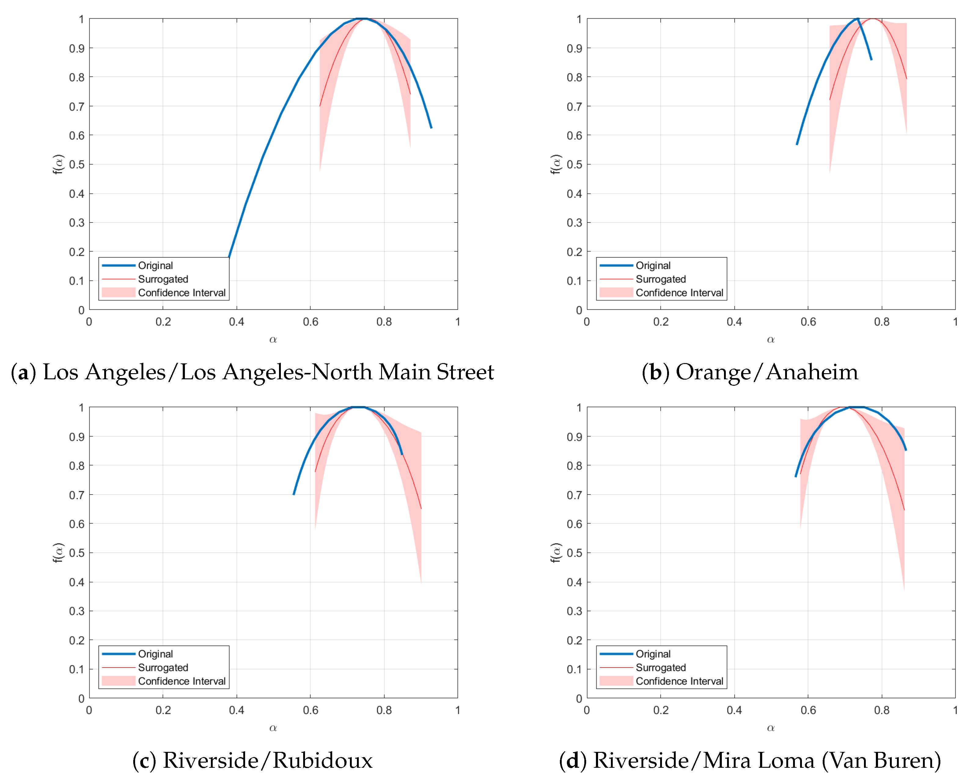
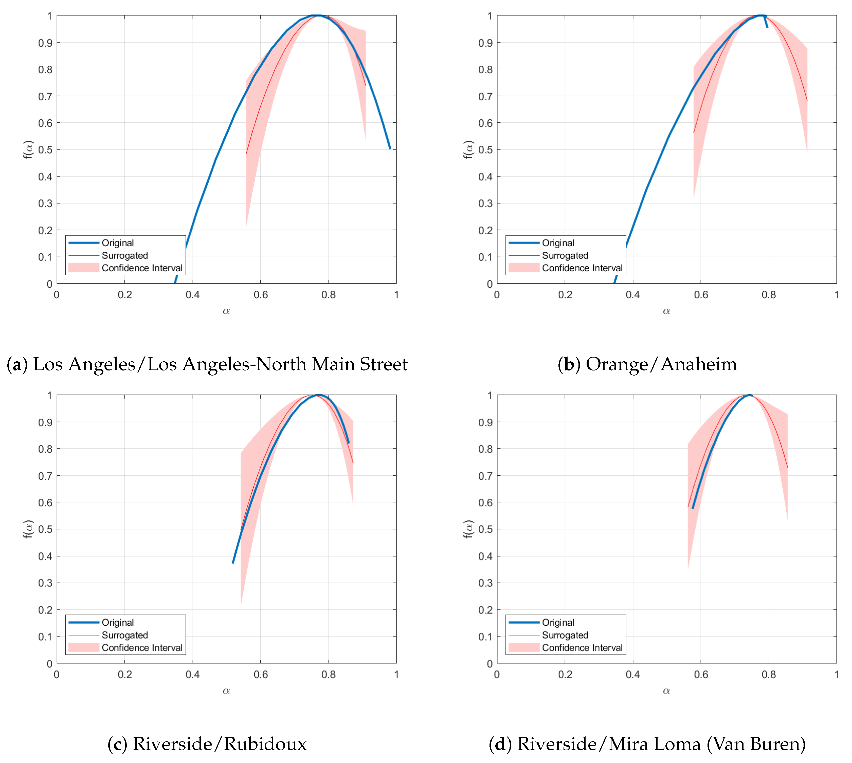
A total of 200 new time series were generated using the Iterative Amplitude Adjusted Fourier Transform (IAAFT) algorithm to identify the sources of multifractality. Figure 12 presents the singularity spectrum for the P M 2.5 -AQI pair. It can be observed that the multifractality arising from fat-tailed distributions and temporal correlations is slightly lower than that observed in the original data. This result suggests that both heavy-tailedness and temporal linear correlations contribute to the multifractal behavior; however, a genuine multifractality component remains, accounting for approximately one-third of the total multifractality observed in the spectrum.
For the O 3 -AQI pair (Figure 13), it can be observed that in the Orange/Anaheim, Riverside/Rubidoux, and Riverside/Mira Loma locations, the effects of heavy-tailedness and temporal linear correlations are minimal, indicating that the observed multifractality is almost entirely genuine. In contrast, for Los Angeles/North Main Street, the contribution of heavy-tailedness and temporal correlations accounts for more than two-thirds of the spectrum’s total multifractality.
Finally, for the P M 2.5 - O 3 pair (Figure 14), it can be observed that the multifractality in both Riverside locations is entirely genuine. In contrast, for Los Angeles/North Main Street and Orange/Anaheim, more than half of the observed multifractality can be attributed to genuine sources.

4. Discussion

The findings of this study reveal pronounced multifractal characteristics in the relationships among P M 2.5 , O 3 , and AQI across the analyzed locations in California. These results corroborate earlier studies demonstrating that air pollution dynamics, particularly in densely populated urban environments, exhibit nonlinear and scale-dependent behaviors [16,17,18]. The multifractal signatures identified suggest that pollutant concentrations are influenced by complex interactions among anthropogenic emissions, meteorological variability, and local topography—factors that together produce persistent and antipersistent temporal dependencies in the observed data.
Our results indicate that Los Angeles/North Main Street consistently displayed the highest degree of multifractality, implying a more heterogeneous and irregular temporal structure in pollutant fluctuations. This finding aligns with the conclusions of Liu et al. [18], who emphasized that highly urbanized areas with intense vehicular traffic and industrial activity often exhibit stronger multifractal behavior due to the coexistence of multiple pollution sources and atmospheric feedback mechanisms. Conversely, Riverside/Mira Loma and Riverside/Rubidoux showed lower multifractality, possibly reflecting more localized and homogeneous emission patterns.
The asymmetric multifractal analysis further highlighted that upward and downward trends in P M 2.5 and O 3 are governed by different scaling dynamics, revealing a structural asymmetry in the pollutant interactions. Such asymmetry implies that the processes driving pollution accumulation differ fundamentally from those governing pollutant dissipation. This finding supports the notion proposed by Cao et al. [26] and Alvarez-Ramirez et al. [25] that real-world environmental systems often exhibit directional dependencies, where the response of the system to increases in pollutant concentrations is not symmetric to decreases.
The surrogate data tests also confirmed that a substantial component of the observed multifractality is genuine rather than solely attributable to fat-tailed distributions or temporal autocorrelations. This reinforces the hypothesis that air quality time series possess intrinsic nonlinearities and complex dependencies, suggesting that pollutant dynamics are driven by interactions beyond random fluctuations or simple periodicities. These findings reinforce previous findings that suggest that conventional approaches cannot reveal the nonlinear nature of pollutant behavior [50]. Additionally, these findings support the idea that multifractality in pollutant series is due to both fat-tailed distributions and long-range correlations [51].
From a practical standpoint, these results underscore the limitations of traditional linear or monofractal models in explaining air pollution variability as in Wang [17]. Linear approaches fail to capture the nonlinear coupling between P M 2.5 and O 3 , particularly under varying meteorological and emission regimes which supports Zhang et al. [52]. Consequently, integrating multifractal analysis into air quality modeling frameworks can enhance our ability to detect early warning signals of pollution episodes, improve the calibration of predictive models, and support more adaptive and targeted mitigation policies as suggested by Zhang et al. [52]. This approach may also contribute to developing spatially explicit models capable of identifying pollution hotspots and understanding cross-scale pollutant interactions in complex urban systems.
Although traditional atmospheric dispersion models such as Gaussian plume, Lagrangian particle, and chemical transport models explicitly incorporate meteorological variables, topography, and chemical transformation processes to simulate the physical and chemical dispersion of pollutants, they often assume linearity and may not fully capture the complex, nonlinear, and multi-scale variability observed in real-world air quality data [53,54]. In contrast, multifractal analysis such as presented here provides a complementary statistical perspective by quantifying the scaling properties, intermittency, and long-range correlations inherent in pollutant time series, which are frequently overlooked by deterministic models [17]. Recent studies have demonstrated that integrating multifractal methods with traditional dispersion modeling may enhance the detection of anomalous pollution episodes, improve model calibration, and reveal hidden dependencies between pollutants such as P M 2.5 and O 3 [52,55]. Thus, while multifractal analysis such as the one herein does not replace process-based models, it adds value by uncovering statistical signatures of complexity and nonlinearity that may arise from interactions among meteorological, chemical, and anthropogenic factors. This integrative approach can provide a more comprehensive understanding of air pollution dynamics and inform the development of more robust predictive and management strategies.
Despite these contributions, this study has several limitations. First, the temporal coverage of the dataset (January 2021–August 2024) restricts the ability to fully account for long-term cyclical and interannual effects. Future research should incorporate longer and higher-resolution datasets to better capture the full spectrum of variability which supports the call by Masseran [56]. Second, the analysis focused solely on four Californian locations, limiting the generalizability of the results to regions with differing climatic, geographical, and socioeconomic conditions. Expanding the spatial coverage could reveal whether the multifractal patterns observed here are universal or context-specific. Finally, the study did not explicitly control for meteorological variables such as temperature, humidity, and wind speed, which are known to modulate pollutant dispersion and chemical transformations. Incorporating these exogenous factors into multifractal frameworks could provide a more mechanistic understanding of air pollution dynamics which reinforces the claim that Yang et al. [57].
As suggested above, there are many areas of opportunity for future research. For instance, one might expand the region of consideration to understand spillovers from one region to another. As wind moves atmospheric content from one region to another, researchers can better understand the impact that one region has on another. Second, including additional meteorological features to the model may help improve the forecasting of particulate matter. With more citizen scientists deploying air-quality monitoring systems, additional data is ever increasing allowing researchers to include conduct better feature engineering. Finally, there is an opportunity to combine the work that is done with respect to modeling particulate matter, greenhouse gas emissions, and regional health effects.
In summary, the results of this research demonstrate that multifractality is an inherent feature of the relationships among P M 2.5 , O 3 , and AQI in California’s urban environments. The evidence of genuine multifractality, asymmetry, and persistent correlations highlights the complex, nonlinear, and multi-scale nature of air pollution processes. These findings contribute to a deeper understanding of environmental complexity and suggest that multifractal-based approaches can serve as powerful analytical tools for advancing air quality modeling, urban sustainability, and public health protection.

5. Conclusions

This study applied the Asymmetric Multifractal Detrending Moving Average (A-MFDMA) method to examine the relationships among P M 2.5 , O 3 , and AQI across four urban locations in California: Los Angeles/North Main Street, Orange/Anaheim, Riverside/Rubidoux, and Riverside/Mira Loma. The approach enabled a detailed exploration of the asymmetric multifractal correlations in air quality time series, capturing both upward and downward trends in pollutant dynamics.
The results demonstrate that all analyzed pairs— P M 2.5 -AQI, O 3 -AQI, and P M 2.5 - O 3 —exhibit significant multifractality, with notable asymmetry across trends and locations. Los Angeles/North Main Street showed the highest degree of multifractality, consistent with the complex emission patterns characteristic of large metropolitan areas. The surrogate data analysis confirmed that a substantial portion of the observed multifractality is genuine, indicating intrinsic nonlinearities and complex dependencies among pollutants rather than artifacts of heavy-tailed distributions or linear correlations.
These findings underscore the limitations of conventional linear models for air quality assessment and highlight the relevance of multifractal frameworks in capturing the nonlinear and scale-dependent behavior of atmospheric pollutants. Incorporating such multifractal insights into predictive and policy-oriented models can improve early detection of pollution episodes, enhance the design of adaptive mitigation strategies, and strengthen public health protection measures.
Overall, this research contributes to a deeper understanding of the complex and asymmetric dynamics underlying air pollution and provides a methodological foundation for future studies aiming to develop robust, multifractal-based approaches to environmental monitoring and urban sustainability.

Author Contributions

W.K.: Conceptualization, Methodology, Software, Formal Analysis, Data curation, writing—original draft preparation, writing—review and editing. M.C.M.: Conceptualization, Methodology, Formal Analysis, writing—original draft preparation, writing—review and editing. All authors have read and agreed to the published version of the manuscript.

Funding

This research received no external funding.

Data Availability Statement

The original contributions presented in this study are included in the article. Further inquiries can be directed to the corresponding author.

Conflicts of Interest

The authors declare no conflicts of interest.

Appendix A. Calculating the AQI

The AQI is the highest value calculated for each pollutant as follows:
1.
Identify the highest concentration among all of the monitors within each reporting area and truncate as follows:
Ozone (ppm)—truncate to 3 decimal places.
P M 2.5 (µg/m3)—truncate to 1 decimal place.
P M 10 (µg/m3)—truncate to integer.
CO (ppm)—truncate to 1 decimal place.
S O 2 (ppb)—truncate to integer.
N O 2 (ppb)—truncate to integer.
2.
Using Figure A1, find the two breakpoints that contain the concentration.
3.
Equation (1), calculate the index.
4.
Round the index to the nearest integer.
I p = I H i I L o B P H i B P L o ( C p B P L o ) + I L o
where
I p = the index for pollutant p.
C p = the truncated concentration of pollutant p.
B P H i = the concentration breakpoint that is greater than or equal to C p .
B P L o = the concentration breakpoint that is less than or equal to C p .
I H i = the AQI value corresponding to B P H i .
I L o = the AQI value corresponding to B P L o .
Figure A1. AQI Basics for Ozone and Particle Pollution. Source: United States Environmental Protection Agency (https://www.airnow.gov/aqi/aqi-basics/ accessed on 4 November 2025).
Fractalfract 09 00821 g0a1

References

  1. Edo, G.I.; Itoje-akpokiniovo, L.O.; Obasohan, P.; Ikpekoro, V.O.; Samuel, P.O.; Jikah, A.N.; Nosu, L.C.; Ekokotu, H.A.; Ugbune, U.; Oghroro, E.E.A.; et al. Impact of environmental pollution from human activities on water, air quality and climate change. Ecol. Front. 2024, 44, 874–889. [Google Scholar] [CrossRef]
  2. Li, G.; Fang, C.; Wang, S.; Sun, S. The effect of economic growth, urbanization, and industrialization on fine particulate matter (PM2.5) concentrations in China. Environ. Sci. Technol. 2016, 50, 11452–11459. [Google Scholar] [CrossRef]
  3. Huszar, P.; Perez, A.P.P.; Bartík, L.; Karlický, J.; Villalba-Pradas, A. Impact of urbanization on fine particulate matter concentrations over central Europe. Atmos. Chem. Phys. 2024, 24, 397–425. [Google Scholar] [CrossRef]
  4. Soni, R.; Nathani, M.; Mishra, R. Comprehensive evaluation of deep ltsf models for forecasting of air quality index. In Proceedings of the 2024 IEEE International Conference on Big Data (BigData), Washington, DC, USA, 15–18 December 2024; IEEE: New York, NY, USA, 2024; pp. 4410–4419. [Google Scholar]
  5. Guo, Z.; Jing, X.; Ling, Y.; Yang, Y.; Jing, N.; Yuan, R.; Liu, Y. Optimized air quality management based on air quality index prediction and air pollutants identification in representative cities in China. Sci. Rep. 2024, 14, 17923. [Google Scholar] [CrossRef]
  6. Manisalidis, I.; Stavropoulou, E.; Stavropoulos, A.; Bezirtzoglou, E. Environmental and health impacts of air pollution: A review. Front. Public Health 2020, 8, 14. [Google Scholar] [CrossRef]
  7. Shoaib, M.; Pechuho, T.; Safdar, M.; Islam, R.; Durrani, F.; Rashid, S.; Khan, K.N.; Chohan, A.A. Air pollution and climate change: A dual threat to ecosystems and human health. J. Med. Health Sci. Rev. 2025, 2. [Google Scholar] [CrossRef]
  8. World Health Organization. What Are the WHO Air Quality Guidelines? Improving Health by Reducing Air Pollution. 2021. Available online: https://www.who.int/news-room/feature-stories/detail/what-are-the-who-air-quality-guidelines#:~:text=What%20do%20the%20guidelines%20recommend,evaluation%20of%20current%20scientific%20evidence (accessed on 4 November 2025).
  9. U.S. Environmental Protection Agency. Air Quality Data. 2024. Available online: https://www.epa.gov/outdoor-air-quality-data (accessed on 4 November 2025).
  10. Hou, J.; Wang, Y.; Zhang, X.; Qiu, L.; Gao, T. The effect of visibility on green space recovery, perception and preference. Trees For. People 2024, 16, 100538. [Google Scholar] [CrossRef]
  11. Klingberg, J.; Broberg, M.; Strandberg, B.; Thorsson, P.; Pleijel, H. Influence of urban vegetation on air pollution and noise exposure—A case study in Gothenburg, Sweden. Sci. Total Environ. 2017, 599, 1728–1739. [Google Scholar] [CrossRef]
  12. Lopes, H.S.; Vidal, D.G.; Cherif, N.; Silva, L.; Remoaldo, P.C. Green infrastructure and its influence on urban heat island, heat risk, and air pollution: A case study of Porto (Portugal). J. Environ. Manag. 2025, 376, 124446. [Google Scholar] [CrossRef]
  13. Han, L.; Zhang, R.; Wang, J.; Cao, S.J. Spatial synergistic effect of urban green space ecosystem on air pollution and heat island effect. Urban Clim. 2024, 55, 101940. [Google Scholar] [CrossRef]
  14. Arriazu-Ramos, A.; Santamaría, J.M.; Monge-Barrio, A.; Bes-Rastrollo, M.; Gutierrez Gabriel, S.; Benito Frias, N.; Sánchez-Ostiz, A. Health Impacts of Urban Environmental Parameters: A Review of Air Pollution, Heat, Noise, Green Spaces and Mobility. Sustainability 2025, 17, 4336. [Google Scholar] [CrossRef]
  15. Nieuwenhuijsen, M.J. New urban models for more sustainable, liveable and healthier cities post COVID-19; reducing air pollution, noise and heat island effects and increasing green space and physical activity. Environ. Int. 2021, 157, 106850. [Google Scholar] [CrossRef]
  16. Zhang, C.; Ni, Z.; Ni, L.; Li, J.; Zhou, L. Asymmetric multifractal detrending moving average analysis in time series of PM2. 5 concentration. Phys. A Stat. Mech. Its Appl. 2016, 457, 322–330. [Google Scholar] [CrossRef]
  17. Wang, Q. Multifractal characterization of air polluted time series in China. Phys. A Stat. Mech. Its Appl. 2019, 514, 167–180. [Google Scholar] [CrossRef]
  18. Liu, C.; Liang, J.; Li, Y.; Shi, K. Fractal analysis of impact of PM2.5 on surface O3 sensitivity regime based on field observations. Sci. Total Environ. 2023, 858, 160136. [Google Scholar] [CrossRef]
  19. Hurst, H.E. Long-term storage capacity of reservoirs. Trans. Am. Soc. Civ. Eng. 1951, 116, 770–799. [Google Scholar] [CrossRef]
  20. Hurst, H.E. A suggested statistical model of some time series which occur in nature. Nature 1957, 180, 494. [Google Scholar] [CrossRef]
  21. Peng, C.K.; Buldyrev, S.V.; Havlin, S.; Simons, M.; Stanley, H.E.; Goldberger, A.L. Mosaic organization of DNA nucleotides. Phys. Rev. E 1994, 49, 1685. [Google Scholar] [CrossRef]
  22. Peng, C.K.; Buldyrev, S.V.; Goldberger, A.L.; Havlin, S.; Sciortino, F.; Simons, M.; Stanley, H.E. Long-range correlations in nucleotide sequences. Nature 1992, 356, 168–170. [Google Scholar] [CrossRef]
  23. Hu, K.; Ivanov, P.C.; Chen, Z.; Carpena, P.; Stanley, H.E. Effect of trends on detrended fluctuation analysis. Phys. Rev. E 2001, 64, 011114. [Google Scholar] [CrossRef]
  24. Kantelhardt, J.W.; Koscielny-Bunde, E.; Rego, H.H.; Havlin, S.; Bunde, A. Detecting long-range correlations with detrended fluctuation analysis. Phys. A Stat. Mech. Its Appl. 2001, 295, 441–454. [Google Scholar] [CrossRef]
  25. Alvarez-Ramirez, J.; Rodriguez, E.; Echeverria, J.C. A DFA approach for assessing asymmetric correlations. Phys. A Stat. Mech. Its Appl. 2009, 388, 2263–2270. [Google Scholar] [CrossRef]
  26. Cao, G.; Cao, J.; Xu, L. Asymmetric multifractal scaling behavior in the Chinese stock market: Based on asymmetric MF-DFA. Phys. A Stat. Mech. Its Appl. 2013, 392, 797–807. [Google Scholar] [CrossRef]
  27. Ossadnik, S.; Buldyrev, S.; Goldberger, A.; Havlin, S.; Mantegna, R.; Peng, C.; Simons, M.; Stanley, H. Correlation approach to identify coding regions in DNA sequences. Biophys. J. 1994, 67, 64–70. [Google Scholar] [CrossRef]
  28. Kavasseri, R.G.; Nagarajan, R. A multifractal description of wind speed records. Chaos Solitons Fractals 2005, 24, 165–173. [Google Scholar] [CrossRef]
  29. Ivanova, K.; Ausloos, M. Application of the detrended fluctuation analysis (DFA) method for describing cloud breaking. Phys. A Stat. Mech. Its Appl. 1999, 274, 349–354. [Google Scholar] [CrossRef]
  30. Feng, T.; Fu, Z.; Deng, X.; Mao, J. A brief description to different multi-fractal behaviors of daily wind speed records over China. Phys. Lett. A 2009, 373, 4134–4141. [Google Scholar] [CrossRef]
  31. Jiang, L.; Zhang, J.; Liu, X.; Li, F. Multi-fractal scaling comparison of the air temperature and the surface temperature over China. Phys. Stat. Mech. Its Appl. 2016, 462, 783–792. [Google Scholar] [CrossRef]
  32. Vitanov, N.K.; Yankulova, E.D. Multifractal analysis of the long-range correlations in the cardiac dynamics of Drosophila melanogaster. Chaos Solitons Fractals 2006, 28, 768–775. [Google Scholar] [CrossRef]
  33. Bunde, A.; Havlin, S.; Kantelhardt, J.W.; Penzel, T.; Peter, J.H.; Voigt, K. Correlated and uncorrelated regions in heart-rate fluctuations during sleep. Phys. Rev. Lett. 2000, 85, 3736. [Google Scholar] [CrossRef]
  34. Ashkenazy, Y.; Ivanov, P.C.; Havlin, S.; Peng, C.K.; Goldberger, A.L.; Stanley, H.E. Magnitude and sign correlations in heartbeat fluctuations. Phys. Rev. Lett. 2001, 86, 1900. [Google Scholar] [CrossRef]
  35. Zheng, H.; Song, W.; Wang, J. Detrended fluctuation analysis of forest fires and related weather parameters. Phys. Stat. Mech. Its Appl. 2008, 387, 2091–2099. [Google Scholar] [CrossRef]
  36. Li, Z.Y.; Liu, H.; Zhao, X.P.; Tao, W.Q. A multi-level fractal model for the effective thermal conductivity of silica aerogel. J.-Non-Cryst. Solids 2015, 430, 43–51. [Google Scholar] [CrossRef]
  37. Shivakumara, P.; Wu, L.; Lu, T.; Tan, C.L.; Blumenstein, M.; Anami, B.S. Fractals based multi-oriented text detection system for recognition in mobile video images. Pattern Recognit. 2017, 68, 158–174. [Google Scholar] [CrossRef]
  38. Tang, Z.; Wu, X.; Fu, B.; Chen, W.; Feng, H. Fast face recognition based on fractal theory. Appl. Math. Comput. 2018, 321, 721–730. [Google Scholar] [CrossRef]
  39. Khalajmasoumi, M.; Sadeghi, B.; Carranza, E.J.M.; Sadeghi, M. Geochemical anomaly recognition of rare earth elements using multi-fractal modeling correlated with geological features, Central Iran. J. Geochem. Explor. 2017, 181, 318–332. [Google Scholar] [CrossRef]
  40. Masugi, M. Multi-fractal analysis of IP-network traffic based on a hierarchical clustering approach. Commun. Nonlinear Sci. Numer. Simul. 2007, 12, 1316–1325. [Google Scholar] [CrossRef]
  41. Huang, L.Y.; Wang, S.P. Improved multi-fractal network traffic model and its performance analysis. J. China Univ. Posts Telecommun. 2011, 18, 102–107. [Google Scholar] [CrossRef]
  42. Quan, W.; Wang, H.; Liu, X.; Zhang, S. Multi-fractal analysis for pavement roughness evaluation. Procedia-Soc. Behav. Sci. 2013, 96, 2684–2691. [Google Scholar] [CrossRef]
  43. Aggarwal, S.K.; Pastén, D.; Khan, P.K. Multifractal analysis of 2001 Mw7. 7 Bhuj earthquake sequence in Gujarat, western India. Phys. Stat. Mech. Its Appl. 2017, 488, 177–186. [Google Scholar] [CrossRef]
  44. Veltri, M.; Severino, G.; De Bartolo, S.; Fallico, C.; Santini, A. Scaling analysis of water retention curves: A multi-fractal approach. Procedia Environ. Sci. 2013, 19, 618–622. [Google Scholar] [CrossRef]
  45. Fan, X.; Lv, X.; Yin, J.; Tian, L.; Liang, J. Multifractality and market efficiency of carbon emission trading market: Analysis using the multifractal detrended fluctuation technique. Appl. Energy 2019, 251, 113333. [Google Scholar] [CrossRef]
  46. Zhang, C.; Ni, Z.; Ni, L. Multifractal detrended cross-correlation analysis between PM2. 5 and meteorological factors. Phys. Stat. Mech. Its Appl. 2015, 438, 114–123. [Google Scholar] [CrossRef]
  47. Cárdenas-Moreno, P.; Moreno-Torres, L.; Lovallo, M.; Telesca, L.; Ramírez-Rojas, A. Spectral, multifractal and informational analysis of PM10 time series measured in Mexico City Metropolitan Area. Phys. Stat. Mech. Its Appl. 2021, 565, 125545. [Google Scholar] [CrossRef]
  48. Kantelhardt, J.W.; Zschiegner, S.A.; Koscielny-Bunde, E.; Havlin, S.; Bunde, A.; Stanley, H.E. Multifractal detrended fluctuation analysis of nonstationary time series. Phys. Stat. Mech. Its Appl. 2002, 316, 87–114. [Google Scholar] [CrossRef]
  49. Podobnik, B.; Grosse, I.; Horvatić, D.; Ilic, S.; Ivanov, P.C.; Stanley, H.E. Quantifying cross-correlations using local and global detrending approaches. Eur. Phys. J. B 2009, 71, 243–250. [Google Scholar] [CrossRef]
  50. Perišić, M.; Vuković, G.; Stanišić, S.M. Multifractal Characteristics of Criteria Air Pollutant Time Series in Urban Areas. In Proceedings of the Sinteza 2020-International Scientific Conference on Information Technology and Data Related Research, Stanford, CA, USA, 1–2 August 2020; Singidunum University: Belgrade, Serbia, 2020; pp. 29–34. [Google Scholar]
  51. Dong, Q.; Wang, Y.; Li, P. Multifractal behavior of an air pollutant time series and the relevance to the predictability. Environ. Pollut. 2017, 222, 444–457. [Google Scholar] [CrossRef]
  52. Zhang, J.; Li, Y.; Liu, C.; Wu, B.; Shi, K. A study of cross-correlations between PM2.5 and O3 based on Copula and Multifractal methods. Phys. Stat. Mech. Its Appl. 2022, 589, 126651. [Google Scholar] [CrossRef]
  53. Seinfeld, J.H.; Pandis, S.N. Atmospheric Chemistry and Physics: From Air Pollution to Climate Change; John Wiley & Sons: Hoboken, NJ, USA, 2016. [Google Scholar]
  54. Holmes, N.S.; Morawska, L. A review of dispersion modelling and its application to the dispersion of particles: An overview of different dispersion models available. Atmos. Environ. 2006, 40, 5902–5928. [Google Scholar] [CrossRef]
  55. Wu, B.; Liu, C.; Zhang, J.; Du, J.; Shi, K. The multifractal evaluation of PM2.5-O3 coordinated control capability in China. Ecol. Indic. 2021, 129, 107877. [Google Scholar] [CrossRef]
  56. Masseran, N. Multifractal characteristics on temporal maximum of air pollution series. Mathematics 2022, 10, 3910. [Google Scholar] [CrossRef]
  57. Yang, Z.; Yang, J.; Li, M.; Chen, J.; Ou, C.Q. Nonlinear and lagged meteorological effects on daily levels of ambient PM2.5 and O3: Evidence from 284 Chinese cities. J. Clean. Prod. 2021, 278, 123931. [Google Scholar] [CrossRef]
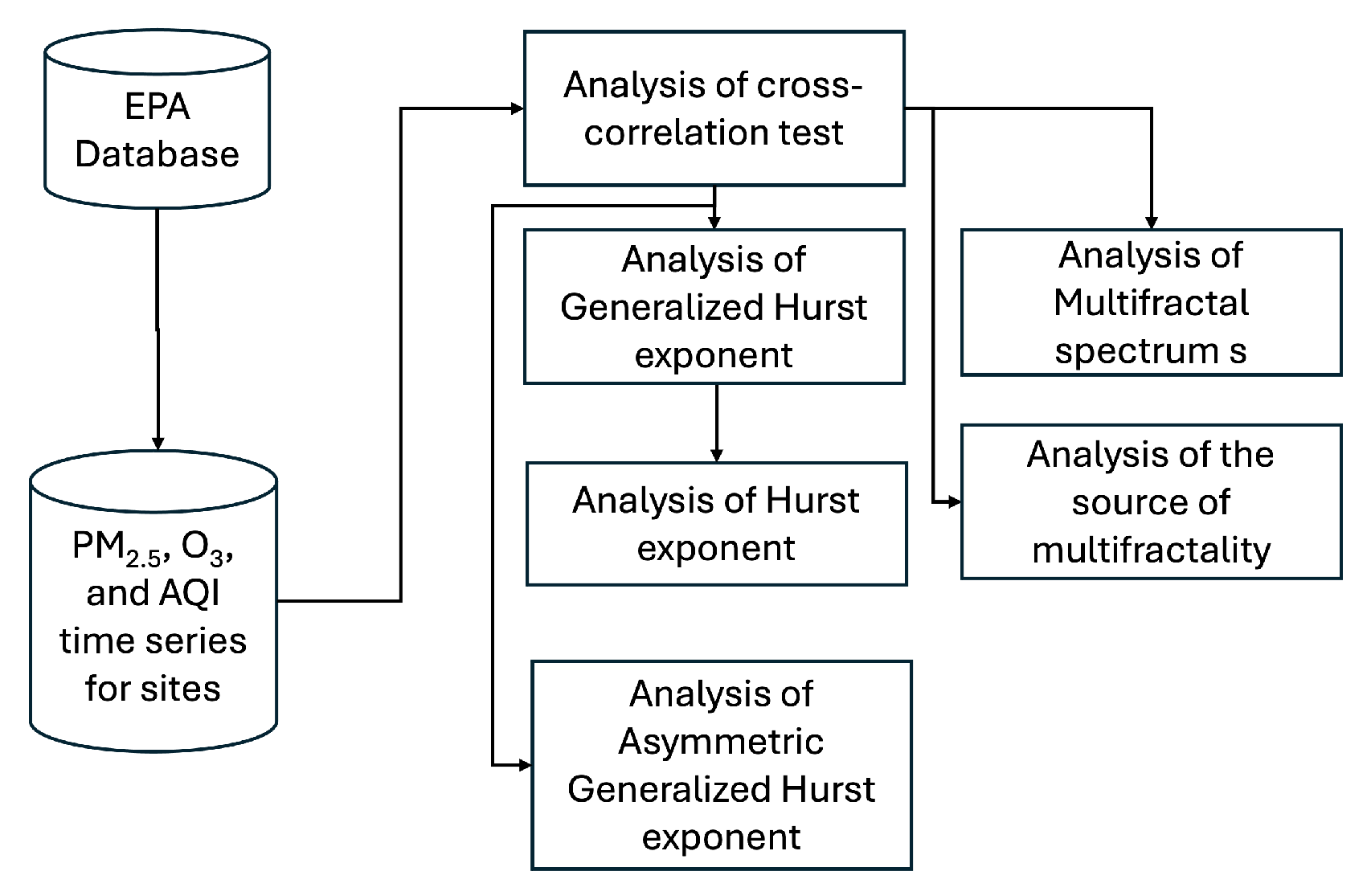
Figure 1. Methodological Framework of the Study.
Fractalfract 09 00821 g001
Figure 2. Evolution of P M 2.5 concentrations (blue) and AQI values (orange) for the four selected study locations. Note: (a) Los Angeles/Los Angeles-North Main Street, (b) Orange/Anaheim, (c) Riverside/Rubidoux, and (d) Riverside/Mira Loma (Van Buren). The P M 2.5 concentrations are expressed in μg/m3 and AQI index ranging 0–200.
Fractalfract 09 00821 g002
Figure 3. Evolution of Ozone concentrations (blue) and AQI values (orange) for the four selected study locations. Note: (a) Los Angeles/Los Angeles-North Main Street, (b) Orange/Anaheim, (c) Riverside/Rubidoux, and (d) Riverside/Mira Loma (Van Buren). The O 3 are expressed in ppm (parts per million) and AQI index ranging 0–200.
Fractalfract 09 00821 g003
Figure 4. Relationship between daily P M 2.5 concentrations and Ozone levels for each location over the study period. Note: (a) Los Angeles/Los Angeles-North Main Street, (b) Orange/Anaheim, (c) Riverside/Rubidoux, and (d) Riverside/Mira Loma (Van Buren). The P M 2.5 concentrations are expressed in μg/m3, and O 3 in ppm (parts per million).
Fractalfract 09 00821 g004
Figure 5. Cross-correaltion test for the P M 2.5 -AQI, Ozone-AQI, and P M 2.5 -Ozone in all the studied locations.
Fractalfract 09 00821 g005
Figure 6. Generalized Hurst exponent ( H x y (q)) for the P M 2.5 -AQI, Ozone-AQI, and P M 2.5 -Ozone in all the studied locations.
Fractalfract 09 00821 g006
Figure 7. Hurst exponent ( H x (2)) and confidence interval at 95% for the P M 2.5 -AQI, Ozone-AQI, and P M 2.5 -Ozone in all the studied locations.
Fractalfract 09 00821 g007
Figure 8. Singularity spectrum for all locations, illustrating the relationship between the singularity strength ( α ) and its corresponding fractal dimension ( f ( α ) ) in all the studied locations.
Fractalfract 09 00821 g008
Figure 9. Generalized Hurst exponent ( H x y (q)) for P M 2.5 -AQI under Upward and downward trend of P M 2.5 , in all the studied locations.
Fractalfract 09 00821 g009
Figure 10. Generalized Hurst exponent ( H x y (q)) for Ozone-AQI under Upward and downward trend of Ozone, in all the studied locations.
Fractalfract 09 00821 g010
Figure 11. Generalized Hurst exponent ( H x y (q)) for P M 2.5 -Ozone under Upward and downward trend of P M 2.5 , in all the studied locations.
Fractalfract 09 00821 g011
Figure 12. Singularity spectrum for all locations, illustrating the relationship between the singularity strength ( α ) and fractal dimension ( f ( α ) ) and surrogate time series with a confidence interval at 95% for P M 2.5 -AQI pairs in all the studied locations.
Fractalfract 09 00821 g012
Figure 13. Singularity spectrum for all locations, illustrating the relationship between the singularity strength ( α ) and fractal dimension ( f ( α ) ) and surrogate time series with a confidence interval at 95% for Ozone–AQI pairs in all the studied locations.
Fractalfract 09 00821 g013
Figure 14. Singularity spectrum for all locations, illustrating the relationship between the singularity strength ( α ) and fractal dimension ( f ( α ) ) and surrogate time series with a confidence interval at 95% for P M 2.5 -Ozone pairs in all the studied locations.
Fractalfract 09 00821 g014
Table 1. Descriptive Statistics of P M 2.5 , O 3 and AQI for period January 2021 to August 2024.
PM 2.5 AQI ( PM 2.5 )
NMSARMLNMSARML
Average11.309.6211.4613.0151.3145.6751.1955.09
St. Dev6.285.576.867.1616.5617.5118.0217.95
Min1.700.101.501.109.001.008.006.00
Max62.3050.7082.1085.10156.00138.00170.00172.00
OzoneAQI (Ozone)
NMSARMLNMSARML
Average0.02850.02800.03520.034542.5836.9664.4262.75
St. Dev0.00940.00890.01250.011816.3210.6940.7437.32
Min0.00150.00150.00150.00254.004.004.005.00
Max0.05310.05220.08030.0738161.00119.00206.00197.00
Descriptive statistics for each air-quality time series across the four monitoring sites: Los Angeles–North Main Street (NMS), Orange–Anaheim (A), Riverside–Rubidoux (R), and Riverside–Mira Loma–Van Buren (ML). Average, St. Dev., Min, and Max denote the mean, standard deviation, minimum, and maximum values of each time series, respectively. The P M 2.5 concentrations are expressed in μg/m3, O 3 in ppm (parts per million), and AQI is an index ranging from 0 to 200.
Disclaimer/Publisher’s Note: The statements, opinions and data contained in all publications are solely those of the individual author(s) and contributor(s) and not of MDPI and/or the editor(s). MDPI and/or the editor(s) disclaim responsibility for any injury to people or property resulting from any ideas, methods, instructions or products referred to in the content.