Time-Domain Dynamics of Fractional Viscoelastic Spinning Disks via Shifted Legendre Polynomials

Abstract

This paper presents a novel algorithm for the dynamic analysis of fractional-order viscoelastic spinning disks in the time domain. The novelty mainly lies in the use of the shifted Legendre polynomial algorithm for the direct time-domain numerical analysis of displacement in two directions for a three-dimensional viscoelastic rotating disk, tackling a more complex and strongly coupled problem than those addressed in previous studies. By using the fractional-order Kelvin–Voigt model to describe the viscoelastic properties of the disk, a system of governing equations with three independent variables is established. For the two ternary unknown functions in the equations, a fractional-order differential operator matrix based on Shifted Legendre polynomials is derived, transforming the original equations into two sets of algebraic equations that are easier to solve. This paper presents an in-depth analysis of the convergence of the Legendre polynomial algorithm, complemented by an investigation of its error characteristics using numerical examples, thereby verifying the method’s accuracy and feasibility. This study can be applied to the dynamic analysis of viscoelastic rotating structures under body force density. The findings provide theoretical support for the optimization and safety assessment of load-bearing rotating components in engineering. And the algorithm demonstrates high accuracy and applicability in handling fractional-order equations in science and engineering.

1. Introduction

In the past few decades, fractional calculus has gained increasing importance in research fields. Compared to integer-order calculus, it has made significant advancements in studying complex physical phenomena with memory effects, hereditary characteristics, and time-dependent behavior [1]. Especially when conducting dynamic analysis of the mechanical behavior of viscoelastic materials, fractional-order models exhibit significant advantages over integer-order models [2]. One key reason is that fractional calculus, with an order between 0 and 1, can accurately characterize the properties of viscoelastic materials, which lie between purely viscous and purely elastic behavior. Moreover, several experimental studies [3,4,5] have demonstrated that fractional-order calculus provides a more realistic representation compared to models relying on multiple integer-order derivatives. As a result, fractional calculus has demonstrated excellent performance and wide applicability in various fields. In the field of mechanics, Shi et al. [6] developed a viscoelastic stress wave propagation model based on fractional-order calculus constitutive relations to characterize the dynamic mechanical properties of low-impedance materials. The model derives the analytical solution of the viscoelastic wave equation while considering the effects of lateral inertia and viscosity on stress wave propagation. The results demonstrate that the application of fractional-order calculus holds significant potential for dynamic mechanical testing of materials, non-destructive evaluation, and seismic exploration. Tang et al. [7] incorporated fractional-order calculus into a multilayer saturated soil consolidation model. By applying the Laplace transform, they obtained semi-analytical solutions for strain, temperature increment, pore water pressure, and settlement. Additionally, they investigated the influence of the fractional-order parameter on thermo-mechanical consolidation behavior. Their findings suggest that the proposed fractional-order model offers significant potential for analyzing the consolidation behavior of viscoelastic materials under complex thermal and mechanical conditions. Mohammad et al. [8] investigated fluid flow around a shrinking permeable cylinder by incorporating fractional-order calculus into the Buongiorno model. Their study examined the dynamic behavior of velocity, temperature, and concentration in nanofluid flow. The results indicate that fractional-order calculus plays a crucial role in complex fluid flow phenomena and has significant practical implications for controlling fluid motion, heat transfer, and mass diffusion. Zheng et al. [9] incorporated several fractional derivative viscoelastic models into a finite element framework via an ABAQUS UMAT 6.14 finite element software subroutine and investigated their convergence behavior and structural responses under static, dynamic and moving loads.

Viscoelastic materials exhibit both viscous and elastic properties, which have increasingly become important in recent years. For example, Geetanjali and Sharma [10] developed a fractional-order generalized thermoelastic diffusion model to study the transient response of a transversely isotropic hollow cylinder, incorporating the effects of nonlocal elasticity. Assuming axial symmetry, the model was reduced to a one-dimensional form and solved using the Laplace transform. The study further examined the influence of the nonlocal parameter and the fractional-order derivative on various thermophysical quantities. Permoon, Haddadpour, and Shakouri [11] investigated the nonlinear vibration of viscoelastic thin cylindrical shells, modeling the material behavior using a fractional-order Kelvin–Voigt constitutive relation. Based on fractional-order Kelvin–Voigt constitutive relation, a system of fractional-order nonlinear differential equations was established by applying the nonlinear Love thin shell theory in conjunction with the Galerkin method. Subsequently, the researchers employed the method of multiple scales to solve the system, thereby obtaining the relationships between amplitude and frequency, as well as phase and frequency. In addition, compared to integer-order models, fractional-order models offer greater flexibility and can better fit experimental data. Moreover, due to their inherent nonlocality, fractional models are well-suited for simulating systems that involve long-term memory effects or complex interactions [12]. Cortés et al. [13] developed a finite element formulation for the transient response of free-layer damping plates in which the viscoelastic damping layer is modeled by a fractional derivative constitutive law, demonstrating that fractional models can accurately capture structural damping behavior while improving computational efficiency. Sun et al. [14] proposed an algorithm based on shifted Legendre polynomials for the dynamic analysis of viscoelastic thickening elastic plates. This study effectively characterizes the internal stress–strain relationship of the plates and analyzes displacement, stress, and bending moments in the time domain. The results highlight the significant potential of fractional-order viscoelastic models in predicting the behavior of complex materials. Zhang et al. [15] formulated the governing equations for nonlinear viscoelastic rods based on fractional-order calculus and solved them in the time domain using a shifted Legendre polynomial algorithm. Furthermore, the study conducted a dynamic analysis of nonlinear viscoelastic rods under various load conditions. The findings provide theoretical support for dynamic response analysis in structural engineering, precision mechanics, and materials science. Hao et al. [16] employed a shifted Legendre polynomial algorithm to solve the governing equations of variable fractional-order cantilever beams in the time domain. Additionally, they analyzed the deflection and stress evolution of cantilever beams made from different materials under various loads. The findings can be extended to other structural forms for higher-precision and more efficient dynamic analysis, with significant potential applications in non-destructive testing and structural health monitoring.

The rotating disk, as a fundamental mechanical structural component, has widespread applications in various fields, including mechanical engineering, aerospace, optics and storage technology, biomedical engineering, and energy. Classic practical examples include turbine disks, hard disks, and rotor assemblies of aircraft. By introducing the concept of viscoelastic materials, the time-dependent behavior and energy dissipation characteristics can be utilized to more accurately study the deformation and stress distribution of rotating disks, thereby optimizing structural design and reducing material fatigue damage. For example, Salehi and Aghae [17] investigated the deformation of viscoelastic disks subjected to magnetic fields, heat flux, and non-uniform asymmetric mechanical loads using the finite difference method and dynamic relaxation method. Shariyat and Mohammadjani [18] derived the governing equations for viscoelastic rotating disks under non-uniform loading based on the Kelvin–Voigt fractional viscoelastic model. They discretized the spatial partial derivatives and time derivatives using the finite difference method. Moreover, it is the first time that this study proposes to employ the shifted Legendre polynomial algorithm for the direct time-domain numerical analysis of the viscoelastic spinning disk. Compared to other methods for solving nonlinear fractional-order partial differential equations, the shifted Legendre polynomial algorithm offers higher stability and simpler computations [19,20].

The innovation of this paper lies in the fact that most existing studies focus on one-dimensional and two-dimensional models [15,16,21], while this paper addresses the three-dimensional model problem in the time domain. Additionally, this study considers a more complex model, involving two unknown functions and a system of governing equations composed of two equations. As the number of governing equations to be solved increases, the associated boundary and initial conditions also grow accordingly. This not only adds to the physical and mathematical complexity of the model but also imposes higher demands on the numerical solution methods. In this study, after discretizing the system of governing equations along with their boundary and initial conditions, the resulting algebraic system exhibits a significantly higher dimensionality and a more complex matrix structure compared to the single-equation case. Consequently, the solution process must address not only the computational burden arising from the increased dimensionality but also pay particular attention to issues of numerical stability and computational efficiency. While most research [22,23,24] focuses on cases involving a single unknown function and a single governing equation.

This paper is organized as follows: Section 2 introduces fundamental definitions and key properties of fractional-order calculus. Section 3 derives the governing equations for the viscoelastic spinning disk. Section 4 details the numerical algorithm used in this study. Section 5 examines the convergence of the proposed algorithm. Section 6 validates its effectiveness through numerical examples. Section 7 investigates the displacement responses of the viscoelastic spinning disk under varying body force density, rotational speeds, and time evolution. Finally, Section 8 summarizes the findings and presents the conclusions.

2. Preliminary

2.1. Definition and Properties of the Fractional Derivative

For fractional calculus, various operators such as Riemann–Liouville, Caputo, and Grünwald–Letnikov operators are defined in sources [25,26,27]. Because the Caputo derivative has advantages over other definitions of fractional-order derivatives in handling initial conditions [28], it is adopted in this paper. When formulating fractional differential equations using the Caputo derivative, the initial conditions can be specified in the same form as those in integer-order differential equations, without the need for additional transformations or reinterpretations required by other definitions. The definition of the Caputo derivative of order $\alpha$ (where $0<\alpha <1$) used in this paper is as follows:

$$\begin{array}{c}\hfill D_t^{\alpha }f\left(t\right)=\left\{\begin{array}{cc}{\displaystyle \frac{{\mathrm{d}}^{m}f\left(t\right)}{\mathrm{d}{t}^m}}\hfill & \alpha =m\in {\mathbb{N}}^{+},\hfill \\ {\displaystyle \frac{1}{\mathrm{\Gamma }(m-\alpha )}}{\int }_{\alpha }^t{\displaystyle \frac{f^{\left(m\right)}\left(\tau \right)}{{(t-\tau )}^{\alpha -m+1}}}\mathrm{d}\tau ,\hfill & 0\le m-1<\alpha <m.\hfill \end{array}\right.\end{array}$$

(1)

where $\mathrm{\Gamma }$ denotes the Gamma function, and $\mathrm{\Gamma }\left(z\right)={\int }_0^{\infty }{e}^{-t}{t}^{z-1}\mathrm{dt}$.

Based on Equation (1), the following equations can be obtained

$$\begin{array}{c}\hfill D_t^{\alpha }{t}^m=\left\{\begin{array}{cc}0\hfill & m\in {\mathbb{N}}_0\mathrm{and}m<\alpha ,\hfill \\ {\displaystyle \frac{\mathrm{\Gamma }(m+1)}{\mathrm{\Gamma }(m+1-\alpha )}}{t}^{m-\alpha }\hfill & m\in {\mathbb{N}}_0\mathrm{and}m\ge \alpha \mathrm{or}m\notin {\mathbb{N}}_0\mathrm{and}m>\alpha .\hfill \end{array}\right.\end{array}$$

(2)

The properties of the Caputo fractional employed in this paper include the following:

• Linearity: The Caputo derivative is a linear operator, meaning that for any two functions $x\left(t\right)$ and $y\left(t\right)$, and constants a and b, we have the following:

  $$\begin{array}{c}\hfill D^{\alpha }[ax\left(t\right)+by\left(t\right)]=a{D}^{\alpha }x\left(t\right)+b{D}^{\alpha }y\left(t\right).\end{array}$$

  (3)
• Commutativity: If the function $x\left(t\right)$ is sufficiently smooth and $\alpha >0$ while m is an integer, then the Caputo fractional derivative can be interchanged with the integer-order derivative.

  $$\begin{array}{c}\hfill D^{\alpha }\left(D^{m}x\left(t\right)\right)=D^m\left(D^{\alpha }x\left(t\right)\right).\end{array}$$

  (4)

2.2. Constitutive Equation of the Linear Viscoelasticity

In mechanical engineering, materials frequently exhibit both elastic and viscous behaviors, which need the development of corresponding models for accurate characterization. Although some classical models, such as the Kelvin–Voigt and Maxwell models, effectively capture distinct viscoelastic characteristics, empirical observations indicate that the relaxation kernels composed of a limited number of exponential terms are insufficient for accurately fitting experimental data. In contrast, fractional-order constitutive equations incorporate non-integer derivatives providing a more comprehensive framework for modeling the stress–strain relationship and effectively addressing phenomena such as creep and relaxation.

Linear viscoelastic material may be modeled by using combinations of different elastic and viscous elements. Fractional constitutive viscoelastic models, such as the four-parameter Zener model [29], the Poynting–Thompson model [30], the fractional Maxwell model [31], and the fractional Kelvin–Voigt model [32], have been used to describe viscoelasticity.

Compared to other models, the fractional-order Kelvin–Voigt model achieves the same or even better fitting accuracy with fewer parameters, reducing modeling complexity. Additionally, unlike classical models, the fractional-order Kelvin–Voigt model more effectively captures the time-scale-dependent behavior of viscoelastic materials [33]. In this paper, the fractional Kelvin–Voigt model is retained to describe the constitutive relationship between stress ($\sigma$) and strain ($ϵ$) which can be expressed, in a one-dimensional case, as follows:

$$\begin{array}{c}\hfill \sigma \left(t\right)=E(1+{\left({\tau }_{\sigma }^E\right)}^{\delta }{D}^{\delta })ϵ\left(t\right),\end{array}$$

(5)

where E is the elastic modulus, ${\tau }_{\sigma }^E$ is the retardation time associated with the fractional Kelvin–Voigt element, and $\delta$ is the order of the Caputo fractional derivative.

3. Establishment of the Fractional-Order Governing Equation of the Viscoelastic Spinning Disk

In this study, we consider a viscoelastic disk spinning at a constant angular velocity $\omega$, subjected to a uniform body force density $F_z$ in the x-direction. Additionally, the disk has a clamped outer boundary and a clamped central axis. In practical rotating disk structures, the central region is typically fixed through a spindle or bearing, forming a rigid connection with the drive system, while the outer edge is often constrained by a housing or a connecting ring to maintain the disk’s balance and stability. Therefore, both the inner and outer edges of the annular plate are assumed to be clamped, which is a common and representative boundary condition in the analysis of annular or disk-type structures [34]. As is shown in Figure 1, the radius and thicknesss of the disk are denoted by R and H, respectively. The symmetry of the body force density and boundary conditions, the variations in the radial and transverse displacement components (u and w, respectively), as well as the radial, tangential, and transverse normal and shear stresses (${\sigma }_r$, ${\sigma }_{\theta }$, ${\sigma }_z$, and ${\tau }_{rz}$, respectively), can be analyzed within a representative radial cross-section, as illustrated in Figure 1. In addition, the material properties of the annular disk include Young’s modulus (E), mass density ($\rho$), Poisson’s ratio ($\nu$), fractional derivative order ($\delta$), and retardation time (${\tau }_{\sigma }^E$). According to three-dimensional elasticity theory [18], the momentum equations in cylindrical coordinates are expressed as follows:

$$\begin{array}{c}\hfill {\sigma }_{r,r}+{\tau }_{rz,z}+{\displaystyle \frac{{\sigma }_r-{\sigma }_{\theta }}{r}}+F_r=\rho \ddot{u},\end{array}$$

(6)

$$\begin{array}{c}\hfill {\tau }_{rz,r}+{\displaystyle \frac{{\tau }_{rz}}{r}}+{\sigma }_{z,z}+F_z=\rho \ddot{w},\end{array}$$

(7)

where $F_r$ and $F_z$ represent the densities of body force in the radial and transverse directions, respectively.

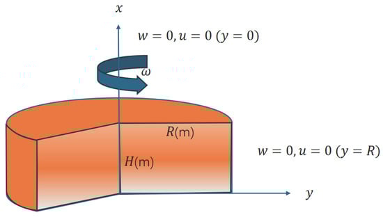
Figure 1. Schematic of a Rotating Viscoelastic Disk.

Based on the generalized Hooke’s stress–strain law and the Babouskos and Katsikadelis generalization [18], the radial, tangential, transverse normal and shear stresses can be obtained as follows

$$\left\{\begin{array}{c}{\sigma }_r\hfill \\ {\sigma }_{\theta }\hfill \\ {\sigma }_z\hfill \\ {\tau }_{rz}\hfill \end{array}\right\}={\displaystyle \frac{E}{(1-2\nu )(1+\nu )}}\left[\begin{array}{cccc}1-\nu & \nu & \nu & 0\\ \nu & 1-\nu & \nu & 0\\ \nu & \nu & 1-\nu & 0\\ 0& 0& 0& {\displaystyle \frac{1-2\nu }{2}}\end{array}\right]\left(1+{\left({\tau }_{\sigma }^E\right)}^{\delta }{D}^{\delta }\right)\left\{\begin{array}{c}{ϵ}_r\\ {ϵ}_{\theta }\\ {ϵ}_z\\ {\gamma }_{rz}\end{array}\right\},$$

(8)

where ${ϵ}_r$,${ϵ}_{\theta }$,${ϵ}_z$ and ${\gamma }_{rz}$ represent radial, tangential, transverse normal, and transverse shear strains, respectively. ${\tau }_{\sigma }^E$ and $\delta$ denote retardation time and order of fractional differentiation, respectively. The governing equations are first derived in cylindrical coordinates $(r,z)$ due to the rotational symmetry. For the subsequent spectral discretization, we adopt the notation $(x,y)$, where r is replaced by y and z is replaced by x.

Additionally, the geometric equations between strain and displacement are as follows:

$$\begin{array}{c}\hfill {ϵ}_r={\displaystyle \frac{\partial u}{\partial y}},{ϵ}_{\theta }={\displaystyle \frac{u}{y}},{ϵ}_z={\displaystyle \frac{\partial w}{\partial x}},{\gamma }_{rz}={\displaystyle \frac{\partial u}{\partial x}}+{\displaystyle \frac{\partial w}{\partial y}}.\end{array}$$

(9)

Substituting Equation (9) into Equation (8), and then applying the result to Equations (6) and (7), the following equations can be obtained:

$$\begin{array}{cc}\hfill & (1-\nu ){\displaystyle \frac{{\partial }^{2}u}{\partial y^2}}+{\displaystyle \frac{1-2\nu }{2}}{\displaystyle \frac{{\partial }^{2}u}{\partial x^2}}+{\displaystyle \frac{1}{2}}{\displaystyle \frac{{\partial }^{2}w}{\partial y\partial x}}+{\displaystyle \frac{1-\nu }{y}}{\displaystyle \frac{\partial u}{\partial y}}-{\displaystyle \frac{1-\nu }{y^2}}u+(1-\nu ){\left({\tau }_{\sigma }^E\right)}^{\delta }{D}^{\delta }\left({\displaystyle \frac{{\partial }^{2}u}{\partial y^2}}\right)\hfill \\ & +{\displaystyle \frac{1-2\nu }{2}}{\left({\tau }_{\sigma }^E\right)}^{\delta }{D}^{\delta }{\displaystyle \frac{{\partial }^{2}u}{\partial x^2}}+{\displaystyle \frac{1}{2}}{\left({\tau }_{\sigma }^E\right)}^{\delta }{D}^{\delta }\left({\displaystyle \frac{{\partial }^{2}w}{\partial y\partial x}}\right)+{\displaystyle \frac{1-\nu }{y}}{\left({\tau }_{\sigma }^E\right)}^{\delta }{D}^{\delta }\left({\displaystyle \frac{\partial u}{\partial y}}\right)-\left({\displaystyle \frac{1-\nu }{y^2}}\right){\left({\tau }_{\sigma }^E\right)}^{\delta }{D}^{\delta }\left(u\right)+{\displaystyle \frac{F_r}{C}}={\displaystyle \frac{\rho \ddot{u}}{C}},\hfill \end{array}$$

(10)

$$\begin{array}{cc}\hfill & {\displaystyle \frac{1-2\nu }{2}}{\displaystyle \frac{{\partial }^{2}w}{\partial y^2}}+(1-\nu ){\displaystyle \frac{{\partial }^{2}w}{\partial x^2}}+{\displaystyle \frac{1}{2}}{\displaystyle \frac{{\partial }^{2}u}{\partial y\partial x}}+{\displaystyle \frac{1-2\nu }{2y}}{\displaystyle \frac{\partial w}{\partial y}}+{\displaystyle \frac{1}{2y}}{\displaystyle \frac{\partial u}{\partial x}}+{\displaystyle \frac{1-2\nu }{2}}{\left({\tau }_{\sigma }^E\right)}^{\delta }{D}^{\delta }\left({\displaystyle \frac{{\partial }^{2}w}{\partial y^2}}\right)\hfill \\ & +(1-\nu ){\left({\tau }_{\sigma }^E\right)}^{\delta }{D}^{\delta }\left({\displaystyle \frac{{\partial }^{2}w}{\partial x^2}}\right)+{\displaystyle \frac{{\left({\tau }_{\sigma }^E\right)}^{\delta }}{2}}{D}^{\delta }\left({\displaystyle \frac{{\partial }^{2}u}{\partial y\partial x}}\right)+{\displaystyle \frac{1-2\nu }{2y}}{\left({\tau }_{\sigma }^E\right)}^{\delta }{D}^{\delta }\left({\displaystyle \frac{\partial w}{\partial y}}\right)+{\displaystyle \frac{1}{2y}}{\left({\tau }_{\sigma }^E\right)}^{\delta }{D}^{\delta }\left({\displaystyle \frac{\partial u}{\partial x}}\right)+F_z={\displaystyle \frac{\rho \ddot{w}}{C}},\hfill \end{array}$$

(11)

where $C={\displaystyle \frac{E}{(1-2\nu )(1+\nu )}}$, $F_r=\rho y{\omega }^2$

4. Shifted Legendre Polynomial Algorithm

In the numerical solution of fractional-order systems, various high-accuracy methods have been widely employed. The finite element method offers excellent geometric flexibility and local refinement capability, making it effective for handling problems involving complex boundaries and heterogeneous materials. However, its convergence rate is typically algebraic, resulting in lower accuracy and efficiency than spectral methods when dealing with smooth and analytic problems [35]. On the other hand, the Chebyshev spectral method takes advantage of the strong clustering of Gauss–Lobatto nodes near the endpoints, enabling it to effectively capture sharp variations and boundary layers close to the domain edges. Moreover, it allows efficient computation through the use of discrete cosine transforms [36]. However, its orthogonal weight function is singular at the endpoints, which necessitates additional weighting or regularization when dealing with Caputo fractional derivatives, thereby increasing the complexity of implementation [37]. In contrast, Legendre polynomials are orthogonal under a unit weight function, and the resulting operational matrices can naturally couple with the Caputo fractional derivative while maintaining extremely high computational accuracy [38]. In this study, shifted Legendre polynomials will be used to approximate the unknown function. Compared to Bernstein polynomials, Legendre polynomials have a simpler weight function. Moreover, when approximating nonlinear singular terms, Legendre polynomials can avoid the redundancy of power function computations while providing faster convergence and more stable numerical calculations [39]. First, using Legendre polynomials as basis functions, the target function $f\left(x\right)$ can be effectively approximated through their orthogonality properties. Then, using the operator matrix to represent the constitutive equation, the original equation is transformed into two sets of algebraic equation systems. The algebraic equation system is then solved to obtain an approximate solution for the parameters. By selecting polynomials of appropriate order, the approximation error can be significantly reduced.

4.1. Shifted Legendre Polynomials

The shifted Legendre polynomial of degree n defined on the interval $[0,1]$ is expressed as follows:

$$\begin{array}{c}\hfill l_{n,i}\left(x\right)=\sum _{i=0}^n{(-1)}^{n+i}{\displaystyle \frac{\mathrm{\Gamma }(n+i+1)}{\mathrm{\Gamma }(n-i+1){\left(\mathrm{\Gamma }(i+1)\right)}^2}}{x}^i.\end{array}$$

(12)

Additionally, shifted Legendre polynomials satisfy the property of orthogonality.

$$\begin{array}{c}\hfill {\int }_0^1{l}_{n,i}\left(x\right)l_{n,j}\left(x\right)dx=\left\{\begin{array}{cc}0\hfill & i\ne j,\hfill \\ {\displaystyle \frac{1}{2i+1}},\hfill & i=j,\hfill \end{array}\right.\end{array}$$

(13)

where $i,j=0,1,\cdots ,n$.

A matrix ${\phi }_n\left(x\right)$ of shifted Legendre polynomials can be expressed as follows:

$$\begin{array}{c}\hfill {\phi }_n\left(x\right)={\left[l_{n,0}\left(x\right),l_{n,1}\left(x\right),\cdots ,l_{n,n}\left(x\right)\right]}^{\top }=A{T}_n\left(x\right),\end{array}$$

(14)

where $T_n\left(x\right)={[1,x,x^2,\cdots ,x^n]}^{\top }$,

$$\begin{array}{c}\hfill A={\left[a_{ij}\right]}_{i,j=0}^n,a_{ij}=\left\{\begin{array}{cc}0\hfill & i<j,\hfill \\ {(-1)}^{i+j}{\displaystyle \frac{\mathrm{\Gamma }(i+j+1)}{\mathrm{\Gamma }(i-j+1)}}\hfill & i\ge j,\hfill \end{array}\right.\end{array}$$

(15)

However, in practical applications, it is often necessary to extend the interval of the Legendre polynomials to $[0,H]$. The following equations represents the shifted Legendre polynomials:

$$\begin{array}{c}\hfill L_{n_1,i}\left(x\right)=\sum _{i=0}^{n_1}{(-1)}^{n_1+i}{\displaystyle \frac{\mathrm{\Gamma }(n_1+i+1)}{\mathrm{\Gamma }(n_1-i+1){\left(\mathrm{\Gamma }(i+1)\right)}^2}}{\left({\displaystyle \frac{x}{H}}\right)}^i=\sum _{i=0}^{n_1}{(-1)}^{n_1+i}{\displaystyle \frac{\mathrm{\Gamma }(n_1+i+1)}{\mathrm{\Gamma }(n_1-i+1){\left(\mathrm{\Gamma }(i+1)\right)}^2}}{\left({\displaystyle \frac{1}{H}}\right)}^i{x}^i,\end{array}$$

(16)

where $x\in [0,H],i=0,1,\cdots ,n_1$. Then, ${\phi }_{n_1}\left(x\right)$ can be transformed as follows:

$$\begin{array}{c}\hfill {\phi }_{n_1}\left(x\right)={[L_{n_1,i}\left(x\right),0\le i\le n_1]}^{\top }=MG\left(x\right),\end{array}$$

(17)

where

$G\left(x\right)={[1,x,\cdots ,x^{n_1}]}^{\top },M={\left[m_{ij}\right]}_{i,j=0}^{n_1},\left[m_{ij}\right]=\left\{\begin{array}{cc}0,\hfill & i<j\hfill \\ {(-1)}^{i+j}{\displaystyle \frac{\mathrm{\Gamma }(i+j+1)}{\mathrm{\Gamma }(i-j+1){\left(\mathrm{\Gamma }(i+1)\right)}^2}}{\left({\displaystyle \frac{1}{H}}\right)}^i,\hfill & i\ge j.\hfill \end{array}\right.$

The following equations can also be obtained:

$$\begin{array}{c}\hfill {\phi }_{n_2}\left(y\right)={[L_{n_2,j}\left(y\right),0\le j\le n_2]}^{\top }=QG\left(y\right)\end{array}$$

(18)

where

$y\in [0,R],G\left(y\right)={[1,y,\cdots ,y^{n_2}]}^{\top }$, $Q={\left[q_{ij}\right]}_{i,j=0}^{n_2}=\left\{\begin{array}{cc}0\hfill & i<j,\hfill \\ {(-1)}^{i+j}{\displaystyle \frac{\mathrm{\Gamma }(i+j+1)}{\mathrm{\Gamma }(i-j+1){\left(\mathrm{\Gamma }(i+1)\right)}^2}}{\left({\displaystyle \frac{1}{R}}\right)}^i\hfill & i\ge j.\hfill \end{array}\right.$

$$\begin{array}{c}\hfill {\phi }_{n_3}\left(t\right)={[L_{n_3,k}\left(t\right),0\le k\le n_3]}^{\top }=NG\left(t\right),\end{array}$$

(19)

where

$t\in [0,K],G\left(t\right)={[1,t,\cdots ,t^{n_3}]}^{\top }$, $N={\left[n_{ij}\right]}_{i,j=0}^{n_3},\left[n_{ij}\right]=\left\{\begin{array}{cc}0,\hfill & i<j\hfill \\ {(-1)}^{i+j}{\displaystyle \frac{\mathrm{\Gamma }(i+j+1)}{\mathrm{\Gamma }(i-j+1){\left(\mathrm{\Gamma }(i+1)\right)}^2}}{\left({\displaystyle \frac{1}{K}}\right)}^i,\hfill & i\ge j\hfill \end{array}\right.$

4.2. Approximation of the Functions and Their Derivatives

Any one-dimensional continuous function defined on the interval $[0,K]$ can be approximated by a finite number of shifted Legendre polynomials.

$$\begin{array}{c}\hfill T\left(t\right)\approx \sum _{k=0}^{n_3}{c}_k{L}_{n_3,k}\left(t\right)=C_1^{\top }{\phi }_{n_3}\left(t\right),\end{array}$$

(20)

where $c_k=⟨T\left(t\right),L_{n_3,k}\left(t\right)⟩$,

$$\begin{array}{c}\hfill C_1^{\top }=[c_0,c_1,\cdots ,c_{n_3}],\end{array}$$

(21)

and ${\phi }_{n_3}\left(t\right)={[L_{n_3,k}\left(t\right),0\le k\le n_3]}^{\top }$ and $c_k$ represents coefficient of shifted Legendre polynomials, $n_3$ denotes the number of terms of shifted Legendre polynomials.

In addition, according to vibration analysis methods [40], a function representing displacement as a function of time can be treated as a separable function. Therefore, the function $u(x,y,t)$ can be separated as follows:

$$\begin{array}{c}\hfill u(x,y,t)=U(x,y)·T\left(t\right),\end{array}$$

(22)

where $U(x,y)\in L^2\left([0,H]\times [0,R]\right),T\left(t\right)\in L^2(0,K)$

The function $U(x,y)$ can be expressed in the following way:

$$\begin{array}{c}\hfill U(x,y)\approx \sum _{i=0}^{n_1}\sum _{j=0}^{n_2}{w}_{ij}{L}_{n_1,i}\left(x\right)L_{n_2,j}\left(y\right)={\phi }_{n_1}^{\top }\left(x\right)W_1{\phi }_{n_2}\left(y\right),\end{array}$$

(23)

where $w_{ij}=⟨U(x,y),L_{n_1,i}\left(x\right)L_{n_2,j}\left(y\right)⟩$ and

$$W_1=[w_0,w_1,\cdots ,w_{n_2}]=\left[\begin{array}{cccc}{w}_{0,0}& w_{0,1}& \cdots & w_{0,n_2}\\ w_{1,0}& w_{1,1}& \cdots & w_{1,n_2}\\ ⋮& ⋮& \ddots & ⋮\\ w_{n_1,0}& w_{n_1,1}& \cdots & w_{n_1,n_2}\end{array}\right],$$

(24)

where $w_j=[w_{0,j},w_{1,j},\cdots ,w_{n_1,j}](j=0,1,\cdots ,n_2)$, $n_1$ and $n_2$ denote the number of terms in the shifted Legendre polynomials, $w_{i,j}$ is coefficient and $W_1$ is the $(n_1+1)\times (n_2+1)$ coefficient matrix to be calculated.

By substituting Equations (20) and (23) into Equation (22), the following results can be obtained:

$$\begin{array}{c}\hfill u(x,y,t)=U(x,y)T\left(t\right)\approx {\phi }_{n_1}^{\top }\left(x\right)W_1{\phi }_{n_2}\left(y\right)C_1^{\top }{\phi }_{n_3}\left(t\right).\end{array}$$

(25)

If there exists a matrix $D_x^m(m\in {\mathbb{N}}^{+})$ such that ${\phi }_{n_1}^{\left(m\right)}\left(x\right)=D_x^m{\phi }_{n_1}\left(x\right)$ holds, then this matrix is called the m-th order differentiation operation matrix for the shifted Legendre polynomials.

The approximation of the derivatives in Equation (17) for the case $m=1$ is derived as follows:

$${\phi }_{n1}^{\prime }\left(x\right)={\left(MG\left(x\right)\right)}^{\prime }=M{G}^{\prime }\left(x\right)=M\left[\begin{array}{c}{1}^{\prime }\\ x^{\prime }\\ ⋮\\ {\left(x^{n_1}\right)}^{\prime }\end{array}\right]=M\left[\begin{array}{c}0\\ 1\\ ⋮\\ n_1{x}^{n_1-1}\end{array}\right]=M{V}_{1}G\left(x\right),$$

(26)

where $V_1={\left[{\nu }_{ij}\right]}_{i,j=0}^{n_1}$, ${\nu }_{ij}=\left\{\begin{array}{cc}0,& i\ne j+1\\ i,& i=j+1\end{array}\right.$

Therefore Equation (26) can be transformed as follows:

$$\begin{array}{c}\hfill {\phi }_{n_1}^{\prime }\left(x\right)=D_x{\phi }_{n_1}\left(x\right)=M{V}_1{M}^{-1}{\phi }_{n_1}\left(x\right),\end{array}$$

(27)

where $D_x=M{V}_1{M}^{-1}$ is a first-order differential operator matrix of the shifted Legendre polynomials.

When $m=2$, it can be obtained

$$\begin{array}{c}\hfill {\phi }_{n_1}^{″}\left(x\right)={\left({\phi }_{n_1}^{\prime }\left(x\right)\right)}^{\prime }=M{V}_1{M}^{-1}{\phi }_{n_1}^{\prime }\left(x\right)={\left(M{V}_1{M}^{-1}\right)}^2{\phi }_{n_1}\left(x\right)=D_x^2{\phi }_{n_1}\left(x\right),\end{array}$$

(28)

where $D_x^2={\left(M{V}_1{M}^{-1}\right)}^2$ is the second-order differential operational matrix of the shifted Legendre polynomials.

Therefore, the m-th order differentiation operation matrix for the shifted Legendre polynomials can be derived.

$$\begin{array}{c}\hfill {\phi }_{n_1}^{\left(m\right)}\left(x\right)={\left(M{V}_1{M}^{-1}\right)}^m{\phi }_{n_1}\left(x\right)=D_x^m{\phi }_{n_1}\left(x\right)\end{array}$$

(29)

$$\begin{array}{c}\hfill {\phi }_{n_2}^{\left(m\right)}\left(y\right)={\left(Q{V}_2{Q}^{-1}\right)}^m{\phi }_{n_2}\left(y\right)=D_y^m{\phi }_{n_2}\left(y\right)\end{array}$$

(30)

$$\begin{array}{c}\hfill {\phi }_{n_3}^{\left(m\right)}\left(t\right)={\left(N{V}_3{N}^{-1}\right)}^m{\phi }_{n_3}\left(t\right)=D_t^m{\phi }_{n_3}\left(t\right)\end{array}$$

(31)

where $V_2={\left[{\nu }_{ij}\right]}_{i,j=0}^{n_2}$, and where $V_3={\left[{\nu }_{ij}\right]}_{i,j=0}^{n_3}$

Accordingly, each term of the constitutive equation can be approximated using the operator matrix as follows:

$$\begin{array}{c}\hfill {\displaystyle \frac{\partial u(x,y,t)}{\partial x}}\approx {\displaystyle \frac{\partial \left({\phi }_{n_1}^{\top }\left(x\right)W_1{\phi }_{n_2}\left(y\right)C_1^{\top }{\phi }_{n_3}\left(t\right)\right)}{\partial x}}={\phi }_{n_1}^{\top }\left(x\right){\left(M{V}_1{M}^{-1}\right)}^{\top }{W}_1{\phi }_{n_2}\left(y\right)C_1^{\top }{\phi }_{n_3}\left(t\right);\end{array}$$

(32)

$$\begin{array}{c}\hfill {\displaystyle \frac{{\partial }^{2}u(x,y,t)}{\partial x^2}}\approx {\displaystyle \frac{{\partial }^2\left({\phi }_{n_1}^{\top }\left(x\right)W_1{\phi }_{n_2}\left(y\right)C_1^{\top }{\phi }_{n_3}\left(t\right)\right)}{\partial x^2}}={\phi }_{n_1}^{\top }\left(x\right){\left({\left(M{V}_1{M}^{-1}\right)}^{\top }\right)}^2{W}_1{\phi }_{n_2}\left(y\right)C_1^{\top }{\phi }_{n_3}\left(t\right);\end{array}$$

(33)

$$\begin{array}{c}\hfill {\displaystyle \frac{{\partial }^{4}u(x,y,t)}{\partial x^4}}\approx {\displaystyle \frac{{\partial }^4\left({\phi }_{n_1}^{\top }\left(x\right)W_1{\phi }_{n_2}\left(y\right)C_1^{\top }{\phi }_{n_3}\left(t\right)\right)}{\partial x^4}}={\phi }_{n_1}^{\top }\left(x\right){\left({\left(M{V}_1{M}^{-1}\right)}^{\top }\right)}^4{W}_1{\phi }_{n_2}\left(y\right)C_1^{\top }{\phi }_{n_3}\left(t\right);\end{array}$$

(34)

$$\begin{array}{c}\hfill {\displaystyle \frac{\partial u(x,y,t)}{\partial y}}\approx {\displaystyle \frac{\partial \left({\phi }_{n_1}^{\top }\left(x\right)W_1{\phi }_{n_2}\left(y\right)C_1^{\top }{\phi }_{n_3}\left(t\right)\right)}{\partial y}}={\phi }_{n_1}^{\top }\left(x\right)W_1\left(Q{V}_2{Q}^{-1}\right){\phi }_{n_2}\left(y\right)C_1^{\top }{\phi }_{n_3}\left(t\right);\end{array}$$

(35)

$$\begin{array}{c}\hfill {\displaystyle \frac{{\partial }^{2}u(x,y,t)}{\partial y^2}}\approx {\displaystyle \frac{{\partial }^2\left({\phi }_{n_1}^{\top }\left(x\right)W_1{\phi }_{n_2}\left(y\right)C_1^{\top }{\phi }_{n_3}\left(t\right)\right)}{\partial y^2}}={\phi }_{n_1}^{\top }\left(x\right)W_1{\left(Q{V}_2{Q}^{-1}\right)}^2{\phi }_{n_2}\left(y\right)C_1^{\top }{\phi }_{n_3}\left(t\right);\end{array}$$

(36)

$$\begin{array}{c}\hfill {\displaystyle \frac{{\partial }^{4}u(x,y,t)}{\partial y^4}}\approx {\displaystyle \frac{{\partial }^4\left({\phi }_{n_1}^{\top }\left(x\right)W_1{\phi }_{n_2}\left(y\right)C_1^{\top }{\phi }_{n_3}\left(t\right)\right)}{\partial y^4}}={\phi }_{n_1}^{\top }\left(x\right)W_1{\left(Q{V}_2{Q}^{-1}\right)}^4{\phi }_{n_2}\left(y\right)C_1^{\top }{\phi }_{n_3}\left(t\right);\end{array}$$

(37)

$$\begin{array}{c}\hfill {\displaystyle \frac{{\partial }^{2}u(x,y,t)}{\partial y\partial x}}\approx {\displaystyle \frac{{\partial }^2\left({\phi }_{n_1}^{\top }\left(x\right)W_1{\phi }_{n_2}\left(y\right)C_1^{\top }{\phi }_{n_3}\left(t\right)\right)}{\partial y\partial x}}={\phi }_{n_1}^{\top }\left(x\right){\left(M{V}_1{M}^{-1}\right)}^{\top }{W}_1\left(Q{V}_2{Q}^{-1}\right){\phi }_{n_2}\left(y\right)C_1^{\top }{\phi }_{n_3}\left(t\right);\end{array}$$

(38)

$$\begin{array}{c}\hfill {\displaystyle \frac{{\partial }^{4}u(x,y,t)}{\partial y^2\partial x^2}}\approx {\displaystyle \frac{{\partial }^4\left({\phi }_{n_1}^{\top }\left(x\right)W_1{\phi }_{n_2}\left(y\right)C_1^{\top }{\phi }_{n_3}\left(t\right)\right)}{\partial y^2\partial x^2}}={\phi }_{n_1}^{\top }\left(x\right){\left({\left(M{V}_1{M}^{-1}\right)}^{\top }\right)}^2{W}_1{\left(Q{V}_2{Q}^{-1}\right)}^2{\phi }_{n_2}\left(y\right)C_1^{\top }{\phi }_{n_3}\left(t\right);\end{array}$$

(39)

$$\begin{array}{c}\hfill {\displaystyle \frac{\partial u(x,y,t)}{\partial t}}\approx {\displaystyle \frac{\partial \left({\phi }_{n_1}^{\top }\left(x\right)W_1{\phi }_{n_2}\left(y\right)C_1^{\top }{\phi }_{n_3}\left(t\right)\right)}{\partial t}}={\phi }_{n_1}^{\top }\left(x\right)W_1{\phi }_{n_2}\left(y\right)C_1^{\top }\left(N{V}_3{N}^{-1}\right){\phi }_{n_3}\left(t\right);\end{array}$$

(40)

$$\begin{array}{c}\hfill {\displaystyle \frac{{\partial }^{2}u(x,y,t)}{\partial t^2}}\approx {\displaystyle \frac{{\partial }^2\left({\phi }_{n_1}^{\top }\left(x\right)W_1{\phi }_{n_2}\left(y\right)C_1^{\top }{\phi }_{n_3}\left(t\right)\right)}{\partial t^2}}={\phi }_{n_1}^{\top }\left(x\right)W_1{\phi }_{n_2}\left(y\right)C_1^{\top }{\left(N{V}_3{N}^{-1}\right)}^2{\phi }_{n_3}\left(t\right);\end{array}$$

(41)

According to the definition of the Caputo fractional derivative, it can be obtained as follows:

$$\begin{array}{cc}\hfill D_t^{\alpha }u(x,y,t)& \approx D_t^{\alpha }\left({\phi }_{n_1}^{\top }\left(x\right)W_1{\phi }_{n_2}\left(y\right)C_1^{\top }{\phi }_{n_3}\left(t\right)\right)={\phi }_{n_1}^{\top }\left(x\right)W_1{\phi }_{n_2}\left(y\right)C_1^{\top }\left(N{V}_3^{\prime }{N}^{-1}\right){\phi }_{n_3}\left(t\right),\hfill \end{array}$$

(42)

where $V_3^{’}={\left[v_{ij}^{\prime }\right]}_{i,j=o}^{n_3},v_{ij}^{\prime }=\left\{\begin{array}{cc}0,& \mathrm{otherwise}\\ {\displaystyle \frac{\mathrm{\Gamma }\left(i\right)}{\mathrm{\Gamma }(i+1)}}{t}^{-\alpha },& i=j,i\ne 1\end{array}\right.$

Therefore, the fractional derivative can be expressed in the following forms:

$$\begin{array}{c}\hfill D_t^{\alpha }{\displaystyle \frac{\partial u(x,y,t)}{\partial x}}\approx {\displaystyle \frac{\partial \left({\phi }_{n_1}^{\top }\left(x\right)W_1{\phi }_{n_2}\left(y\right)C_1^{\top }{D}_t^{\alpha }{\phi }_{n_3}\left(t\right)\right)}{\partial x}}={\phi }_{n_1}^{\top }\left(x\right){\left(M{V}_1{M}^{-1}\right)}^{\top }{W}_1{\phi }_{n_2}\left(y\right)C_1^{\top }\left(N{V}_3^{\prime }{N}^{-1}\right){\phi }_{n_3}\left(t\right);\end{array}$$

(43)

$$\begin{array}{c}\hfill D_t^{\alpha }{\displaystyle \frac{{\partial }^{2}u(x,y,t)}{\partial x^2}}\approx {\displaystyle \frac{{\partial }^2\left({\phi }_{n_1}^{\top }\left(x\right)W_1{\phi }_{n_2}\left(y\right)C_1^{\top }{D}_t^{\alpha }{\phi }_{n_3}\left(t\right)\right)}{\partial x^2}}={\phi }_{n_1}^{\top }\left(x\right){\left({\left(M{V}_1{M}^{-1}\right)}^{\top }\right)}^2{W}_1{\phi }_{n_2}\left(y\right)C_1^{\top }\left(N{V}_3^{\prime }{N}^{-1}\right){\phi }_{n_3}\left(t\right);\end{array}$$

(44)

$$\begin{array}{c}\hfill D_t^{\alpha }{\displaystyle \frac{\partial u(x,y,t)}{\partial y}}\approx {\displaystyle \frac{\partial \left({\phi }_{n_1}^{\top }\left(x\right)W_1{\phi }_{n_2}\left(y\right)C_1^{\top }{D}_t^{\alpha }{\phi }_{n_3}\left(t\right)\right)}{\partial y}}={\phi }_{n_1}^{\top }\left(x\right)W_1\left(Q{V}_2{Q}^{-1}\right){\phi }_{n_2}\left(y\right)C_1^{\top }\left(N{V}_3^{\prime }{N}^{-1}\right){\phi }_{n_3}\left(t\right);\end{array}$$

(45)

$$\begin{array}{cc}\hfill D_t^{\alpha }{\displaystyle \frac{{\partial }^{2}u(x,y,t)}{\partial y^2}}& \approx {\displaystyle \frac{{\partial }^2\left({\phi }_{n_1}^{\top }\left(x\right)W_1{\phi }_{n_2}\left(y\right)C_1^{\top }{D}_t^{\alpha }{\phi }_{n_3}\left(t\right)\right)}{\partial y^2}}={\phi }_{n_1}^{\top }\left(x\right)W_1{\left(Q{V}_2{Q}^{-1}\right)}^2{\phi }_{n_2}\left(y\right)C_1^{\top }\left(N{V}_3^{\prime }{N}^{-1}\right){\phi }_{n_3}\left(t\right);\hfill \end{array}$$

(46)

$$\begin{array}{c}\hfill D_t^{\alpha }{\displaystyle \frac{{\partial }^{2}u(x,y,t)}{\partial y\partial x}}\approx {\displaystyle \frac{{\partial }^2\left({\phi }_{n_1}^{\top }\left(x\right)W_1{\phi }_{n_2}\left(y\right)C_1^{\top }{\phi }_{n_3}\left(t\right)\right)}{\partial y\partial x}}={\phi }_{n_1}^{\top }\left(x\right){\left(M{V}_1{M}^{-1}\right)}^{\top }{W}_1\left(Q{V}_2{Q}^{-1}\right){\phi }_{n_2}\left(y\right)C_1^{\top }\left(N{V}_3^{\prime }{N}^{-1}\right){\phi }_{n_3}\left(t\right);\end{array}$$

(47)

Similarly, based on Equation (25), $w(x,y,t)$ can be transformed as

$$\begin{array}{c}\hfill w(x,y,t)=V(x,y)Z\left(t\right)\approx {\phi }_{n_1}^{\top }\left(x\right)W_2{\phi }_{n_2}\left(y\right)C_2^{\top }{\phi }_{n_3}\left(t\right),\end{array}$$

(48)

where $c_k^{\prime }=⟨Z\left(t\right),L_{n_3,k}\left(t\right)⟩$

$$\begin{array}{c}\hfill C_2^{\top }=\left[c_0^{\prime },c_1^{\prime },\cdots ,c_{n_3}^{\prime }\right],\end{array}$$

(49)

and $c_k^{\prime }$ represents coefficient of shifted Legendre polynomials. In addition, $w_{ij}^{\prime }=$$⟨V(x,y),L_{n_1,i}\left(x\right)L_{n_2,j}\left(y\right)⟩$ and

$$W_2=\left[w_0^{\prime },w_1^{\prime },\cdots ,w_{n_2}^{\prime }\right]=\left[\begin{array}{cccc}{w}_{0,0}^{\prime }& w_{0,1}^{\prime }& \cdots & w_{0,n_2}^{\prime }\\ w_{1,0}^{\prime }& w_{1,1}^{\prime }& \cdots & w_{1,n_2}^{\prime }\\ ⋮& ⋮& \ddots & ⋮\\ w_{n_1,0}^{\prime }& w_{n_1,1}^{\prime }& \cdots & w_{n_1,n_2}^{\prime }\end{array}\right],$$

(50)

where $w_j^{\prime }=[w_{0,j}^{\prime },w_{1,j}^{\prime },\cdots ,w_{n_1,j}^{\prime }](j=0,1,\cdots ,n_2)$, $w_{i,j}^{\prime }$ is coefficient and $W_2$ is the $(n_1+1)\times (n_2+1)$ coefficient matrix to be calculated.

4.3. Transformation of the Governing Equation

By substituting Equations (25) and (32)–(50) into Equations (10) and (11), the following matrix equations can be obtained:

$$\begin{array}{cc}\hfill & \left(1-\nu \right){\phi }_{n_1}^{\top }\left(x\right)W_1{\left(R{V}_2{R}^{-1}\right)}^2{\phi }_{n_2}\left(y\right)C_1^{\top }{\phi }_{n_3}\left(t\right)+{\displaystyle \frac{1-2\nu }{2}}{\phi }_{n_1}^{\top }\left(x\right){\left({\left(M{V}_1{M}^{-1}\right)}^{\top }\right)}^2{W}_1{\phi }_{n_2}\left(y\right)C_1^{\top }{\phi }_{n_3}\left(t\right)\hfill \\ \hfill & +{\displaystyle \frac{1}{2}}{\phi }_{n_1}^{\top }\left(x\right){\left(M{V}_1{M}^{-1}\right)}^{\top }{W}_2\left(R{V}_2{R}^{-1}\right){\phi }_{n_2}\left(y\right)C_2^{\top }{\phi }_{n_3}\left(t\right)+{\displaystyle \frac{1-\nu }{y}}{\phi }_{n_1}^{\top }\left(x\right)W_1\left(R{V}_2{R}^{-1}\right){\phi }_{n_2}\left(y\right)C_1^{\top }{\phi }_{n_3}\left(t\right)\hfill \\ \hfill & -{\displaystyle \frac{1-\nu }{y^2}}{\phi }_{n_1}^{\top }\left(x\right)W_1{\phi }_{n_2}\left(y\right)C_1^{\top }{\phi }_{n_3}\left(t\right)+\left(1-\nu \right){\left({\tau }_{\sigma }^E\right)}^{\delta }{\phi }_{n_1}^{\top }\left(x\right)W_1{\left(R{V}_2{R}^{-1}\right)}^2{\phi }_{n_2}\left(y\right)C_1^{\top }\left(N{V}_3^{\prime }{N}^{-1}\right){\phi }_{n_3}\left(t\right)\hfill \\ \hfill & +{\displaystyle \frac{1-2\nu }{2}}{\left({\tau }_{\sigma }^E\right)}^{\delta }{\phi }_{n_1}^{\top }\left(x\right){\left({\left(M{V}_1{M}^{-1}\right)}^{\top }\right)}^2{W}_1{\phi }_{n_2}\left(y\right)C_1^{\top }\left(N{V}_3^{\prime }{N}^{-1}\right){\phi }_{n_3}\left(t\right)\hfill \\ \hfill & +{\displaystyle \frac{1}{2}}{\left({\tau }_{\sigma }^E\right)}^{\delta }{\phi }_{n_1}^{\top }\left(x\right){\left(M{V}_1{M}^{-1}\right)}^{\top }{W}_2\left(Q{V}_2{Q}^{-1}\right){\phi }_{n_2}\left(y\right)C_2^{\top }\left(N{V}_3^{\prime }{N}^{-1}\right){\phi }_{n_3}\left(t\right)\hfill \\ \hfill & +{\displaystyle \frac{1-\nu }{y}}{\left({\tau }_{\sigma }^E\right)}^{\delta }{\phi }_{n_1}^{\top }\left(x\right)W_1\left(Q{V}_2{Q}^{-1}\right){\phi }_{n_2}\left(y\right)C_1^{\top }\left(N{V}_3^{\prime }{N}^{-1}\right){\phi }_{n_3}\left(t\right)\hfill \\ \hfill & -\left({\displaystyle \frac{1-\nu }{y^2}}\right){\left({\tau }_{\sigma }^E\right)}^{\delta }{\phi }_{n_1}^{\top }\left(x\right)W_1{\phi }_{n_2}\left(y\right)C_1^{\top }\left(N{V}_3^{\prime }{N}^{-1}\right){\phi }_{n_3}\left(t\right)\hfill \\ \hfill & +{\displaystyle \frac{\rho y{\omega }^2}{C}}={\displaystyle \frac{\rho }{C}}{\phi }_{n_1}^{\top }\left(x\right)W_1{\phi }_{n_2}\left(y\right)C_1^{\top }{\left(N{V}_3{N}^{-1}\right)}^2{\phi }_{n_3}\left(t\right);\hfill \end{array}$$

(51)

$$\begin{array}{cc}\hfill & {\displaystyle \frac{1-2\nu }{2}}{\phi }_{n_1}^{\top }\left(x\right)W_2{\left(Q{V}_2{Q}^{-1}\right)}^2{\phi }_{n_2}\left(y\right)C_2^{\top }{\phi }_{n_3}\left(t\right)+\left(1-\nu \right){\phi }_{n_1}^{\top }\left(x\right){\left({\left(M{V}_1{M}^{-1}\right)}^{\top }\right)}^2{W}_2{\phi }_{n_2}\left(y\right)C_2^{\top }{\phi }_{n_3}\left(t\right)\hfill \\ \hfill & +{\displaystyle \frac{1}{2}}{\phi }_{n_1}^{\top }\left(x\right){\left(M{V}_1{M}^{-1}\right)}^{\top }{W}_1\left(Q{V}_2{Q}^{-1}\right){\phi }_{n_2}\left(y\right)C_1^{\top }{\phi }_{n_3}\left(t\right)+{\displaystyle \frac{1-2\nu }{2y}}{\phi }_{n_1}^{\top }\left(x\right)W_2\left(Q{V}_2{Q}^{-1}\right){\phi }_{n_2}\left(y\right)C_2^{\top }{\phi }_{n_3}\left(t\right)\hfill \\ \hfill & +{\displaystyle \frac{1}{2y}}{\phi }_{n_1}^{\top }\left(x\right){\left(M{V}_1{M}^{-1}\right)}^{\top }{W}_1{\phi }_{n_2}\left(y\right)C_1^{\top }{\phi }_{n_3}\left(t\right)+{\displaystyle \frac{1-2\nu }{2}}{\left({\tau }_{\sigma }^E\right)}^{\delta }{\phi }_{n_1}^{\top }\left(x\right)W_2{\left(Q{V}_2{Q}^{-1}\right)}^2{\phi }_{n_2}\left(y\right)C_2^{\top }\left(N{V}_3^{\prime }{N}^{-1}\right){\phi }_{n_3}\left(t\right)\hfill \\ \hfill & +\left(1-\nu \right){\left({\tau }_{\sigma }^E\right)}^{\delta }{\phi }_{n_1}^{\top }\left(x\right){\left({\left(M{V}_1{M}^{-1}\right)}^{\top }\right)}^2{W}_2{\phi }_{n_2}\left(y\right)C_2^{\top }\left(N{V}_3^{\prime }{N}^{-1}\right){\phi }_{n_3}\left(t\right)\hfill \\ \hfill & +{\displaystyle \frac{{\left({\tau }_{\sigma }^E\right)}^{\delta }}{2}}{\phi }_{n_1}^{\top }\left(x\right){\left(M{V}_1{M}^{-1}\right)}^{\top }{W}_1\left(Q{V}_2{Q}^{-1}\right){\phi }_{n_2}\left(y\right)C_1^{\top }\left(N{V}_3^{\prime }{N}^{-1}\right){\phi }_{n_3}\left(t\right)\hfill \\ \hfill & +{\displaystyle \frac{1-2\nu }{2y}}{\left({\tau }_{\sigma }^E\right)}^{\delta }{\phi }_{n_1}^{\top }\left(x\right)W_2\left(Q{V}_2{Q}^{-1}\right){\phi }_{n_2}\left(y\right)C_2^{\top }\left(N{V}_3^{\prime }{N}^{-1}\right){\phi }_{n_3}\left(t\right)\hfill \\ \hfill & +{\displaystyle \frac{1}{2y}}{\left({\tau }_{\sigma }^E\right)}^{\delta }{\phi }_{n_1}^{\top }\left(x\right){\left(M{V}_1{M}^{-1}\right)}^{\top }{W}_1{\phi }_{n_2}\left(y\right)C_1^{\top }\left(N{V}_3^{\prime }{N}^{-1}\right){\phi }_{n_3}\left(t\right)+F_z\hfill \\ \hfill & ={\displaystyle \frac{\rho }{C}}{\phi }_{n_1}^{\top }\left(x\right)W_2{\phi }_{n_2}\left(y\right)C_2^{\top }{\left(N{V}_3{N}^{-1}\right)}^2{\phi }_{n_3}\left(t\right).\hfill \end{array}$$

(52)

In addition, the boundary conditions of a clamped edge can be rewritten as follows:

$$\begin{array}{cc}\hfill u(x,0,t)& \approx {\phi }_{n_1}^{\top }\left(x\right)W_1{\phi }_{n_2}\left(0\right)C_1^{\top }{\phi }_{n_3}\left(t\right)=0(0\le x\le H);\hfill \\ \hfill u(x,R,t)& \approx {\phi }_{n_1}^{\top }\left(x\right)W_1{\phi }_{n_2}\left(R\right)C_1^{\top }{\phi }_{n_3}\left(t\right)=0(0\le x\le H);\hfill \\ \hfill w(x,0,t)& \approx {\phi }_{n_1}^{\top }\left(x\right)W_2{\phi }_{n_2}\left(0\right)C_2^{\top }{\phi }_{n_3}\left(t\right)=0(0\le x\le H);\hfill \\ \hfill w(x,R,t)& \approx {\phi }_{n_1}^{\top }\left(x\right)W_2{\phi }_{n_2}\left(R\right)C_2^{\top }{\phi }_{n_3}\left(t\right)=0(0\le x\le H).\hfill \end{array}$$

(53)

Similarly, the initial conditions can also be transformed as follows:

$$\begin{array}{cc}\hfill {\displaystyle \frac{\partial u(x,y,0)}{\partial t}}& \approx {\phi }_{n_1}^{\top }\left(x\right)W_1{\phi }_{n_2}\left(y\right)C_1^{\top }\left(N{V}_3{N}^{-1}\right){\phi }_{n_3}\left(0\right);\hfill \\ \hfill {\displaystyle \frac{\partial w(x,y,0)}{\partial t}}& \approx {\phi }_{n_1}^{\top }\left(x\right)W_2{\phi }_{n_2}\left(y\right)C_2^{\top }\left(N{V}_3{N}^{-1}\right){\phi }_{n_3}\left(0\right).\hfill \end{array}$$

(54)

Subsequently, the intervals $[0,H]$, $[0,R]$, $[0,K]$ are divided into n equal parts, yielding the discrete points $x_i$, $y_j$, and $t_k$, where $x_i=i{\displaystyle \frac{H}{n_1}}$, $y_j=j{\displaystyle \frac{R}{n_2}}$, $t_k=k{\displaystyle \frac{K}{n_3}}(i=0,\cdots ,n_1$; $j=0,\cdots ,n_2$; $k=0,\cdots ,n_3$). By substituting these discrete points into Equations (51)–(54), a nonlinear system of equations ${\displaystyle f_m\left(X\right)=0,(m=1,\cdots ,\sum _{i=1}^8{m}_i)}$ can be obtained as follows:

$$\begin{array}{cc}\hfill f_{m_1}\left(X\right)& =\left(1-\nu \right){\phi }_{n_1}^{\top }\left(x_i\right)W_1{\left(Q{V}_2{Q}^{-1}\right)}^2{\phi }_{n_2}\left(y_j\right)C_1^{\top }{\phi }_{n_3}\left(t_k\right)\hfill \\ & +{\displaystyle \frac{1-2\nu }{2}}{\phi }_{n_1}^{\top }\left(x_i\right){\left({\left(M{V}_1{M}^{-1}\right)}^{\top }\right)}^2{W}_1{\phi }_{n_2}\left(y_j\right)C_1^{\top }{\phi }_{n_3}\left(t_k\right)\hfill \\ \hfill & +{\displaystyle \frac{1}{2}}{\phi }_{n_1}^{\top }\left(x_i\right){\left(M{V}_1{M}^{-1}\right)}^{\top }{W}_2\left(Q{V}_2{Q}^{-1}\right){\phi }_{n_2}\left(y_j\right)C_2^{\top }{\phi }_{n_3}\left(t_k\right)\hfill \\ & +{\displaystyle \frac{1-\nu }{y_j}}{\phi }_{n_1}^{\top }\left(x_i\right)W_1\left(Q{V}_2{Q}^{-1}\right){\phi }_{n_2}\left(y_j\right)C_1^{\top }{\phi }_{n_3}\left(t_k\right)\hfill \\ \hfill & -{\displaystyle \frac{1-\nu }{y_j^2}}{\phi }_{n_1}^{\top }\left(x_i\right)W_1{\phi }_{n_2}\left(y_j\right)C_1^{\top }{\phi }_{n_3}\left(t_k\right)\hfill \\ & +\left(1-\nu \right){\left({\tau }_{\sigma }^E\right)}^{\delta }{\phi }_{n_1}^{\top }\left(x_i\right)W_1{\left(Q{V}_2{Q}^{-1}\right)}^2{\phi }_{n_2}\left(y_j\right)C_1^{\top }\left(N{V}_3^{\prime }{N}^{-1}\right){\phi }_{n_3}\left(t_k\right)\hfill \\ \hfill & +{\displaystyle \frac{1-2\nu }{2}}{\left({\tau }_{\sigma }^E\right)}^{\delta }{\phi }_{n_1}^{\top }\left(x_i\right){\left({\left(M{V}_1{M}^{-1}\right)}^{\top }\right)}^2{W}_1{\phi }_{n_2}\left(y_j\right)C_1^{\top }\left(N{V}_3^{\prime }{N}^{-1}\right){\phi }_{n_3}\left(t_k\right)\hfill \\ \hfill & +{\displaystyle \frac{1}{2}}{\left({\tau }_{\sigma }^E\right)}^{\delta }{\phi }_{n_1}^{\top }\left(x_i\right){\left(M{V}_1{M}^{-1}\right)}^{\top }{W}_2\left(Q{V}_2{Q}^{-1}\right){\phi }_{n_2}\left(y_j\right)C_2^{\top }\left(N{V}_3^{\prime }{N}^{-1}\right){\phi }_{n_3}\left(t_k\right)\hfill \\ \hfill & +{\displaystyle \frac{1-\nu }{y_j}}{\left({\tau }_{\sigma }^E\right)}^{\delta }{\phi }_{n_1}^{\top }\left(x_i\right)W_1\left(Q{V}_2{Q}^{-1}\right){\phi }_{n_2}\left(y_j\right)C_1^{\top }\left(N{V}_3^{\prime }{N}^{-1}\right){\phi }_{n_3}\left(t_k\right)\hfill \\ \hfill & -\left({\displaystyle \frac{1-\nu }{y_j^2}}\right){\left({\tau }_{\sigma }^E\right)}^{\delta }{\phi }_{n_1}^{\top }\left(x_i\right)W_1{\phi }_{n_2}\left(y_j\right)C_1^{\top }\left(N{V}_3^{\prime }{N}^{-1}\right){\phi }_{n_3}\left(t_k\right)\hfill \\ \hfill & +{\displaystyle \frac{\rho y_j{\omega }^2}{C}}-{\displaystyle \frac{\rho }{C}}{\phi }_{n_1}^{\top }\left(x_i\right)W_1{\phi }_{n_2}\left(y_j\right)C_1^{\top }{\left(N{V}_3{N}^{-1}\right)}^2{\phi }_{n_3}\left(t_k\right)\hfill \\ & =0\left(m_1=0,1,\cdots ,(n_1+1)\ast (n_2+1)\ast (n_3+1)\right)\hfill \\ \hfill f_{m_2}\left(X\right)& ={\displaystyle \frac{1-2\nu }{2}}{\phi }_{n_1}^{\top }\left(x_i\right)W_2{\left(Q{V}_2{Q}^{-1}\right)}^2{\phi }_{n_2}\left(y_j\right)C_2^{\top }{\phi }_{n_3}\left(t_k\right)\hfill \\ & +\left(1-\nu \right){\phi }_{n_1}^{\top }\left(x_i\right){\left({\left(M{V}_1{M}^{-1}\right)}^{\top }\right)}^2{W}_2{\phi }_{n_2}\left(y_j\right)C_2^{\top }{\phi }_{n_3}\left(t_k\right)\hfill \\ \hfill & +{\displaystyle \frac{1}{2}}{\phi }_{n_1}^{\top }\left(x_i\right){\left(M{V}_1{M}^{-1}\right)}^{\top }{W}_1\left(Q{V}_2{Q}^{-1}\right){\phi }_{n_2}\left(y_j\right)C_1^{\top }{\phi }_{n_3}\left(t_k\right)\hfill \\ & +{\displaystyle \frac{1-2\nu }{2y_j}}{\phi }_{n_1}^{\top }\left(x_i\right)W_2\left(Q{V}_2{Q}^{-1}\right){\phi }_{n_2}\left(y_j\right)C_2^{\top }{\phi }_{n_3}\left(t_k\right)\hfill \\ \hfill & +{\displaystyle \frac{1}{2y_j}}{\phi }_{n_1}^{\top }\left(x_i\right){\left(M{V}_1{M}^{-1}\right)}^{\top }{W}_1{\phi }_{n_2}\left(y_j\right)C_1^{\top }{\phi }_{n_3}\left(t_k\right)\hfill \\ \hfill & +{\displaystyle \frac{1-2\nu }{2}}{\left({\tau }_{\sigma }^E\right)}^{\delta }{\phi }_{n_1}^{\top }\left(x_i\right)W_2{\left(Q{V}_2{Q}^{-1}\right)}^2{\phi }_{n_2}\left(y_j\right)C_2^{\top }\left(N{V}_3^{\prime }{N}^{-1}\right){\phi }_{n_3}\left(t_k\right)\hfill \\ \hfill & +\left(1-\nu \right){\left({\tau }_{\sigma }^E\right)}^{\delta }{\phi }_{n_1}^{\top }\left(x_i\right){\left({\left(M{V}_1{M}^{-1}\right)}^{\top }\right)}^2{W}_2{\phi }_{n_2}\left(y_j\right)C_2^{\top }\left(N{V}_3^{\prime }{N}^{-1}\right){\phi }_{n_3}\left(t_k\right)\hfill \\ \hfill & +{\displaystyle \frac{{\left({\tau }_{\sigma }^E\right)}^{\delta }}{2}}{\phi }_{n_1}^{\top }\left(x_i\right){\left(M{V}_1{M}^{-1}\right)}^{\top }{W}_1\left(Q{V}_2{Q}^{-1}\right){\phi }_{n_2}\left(y_j\right)C_1^{\top }\left(N{V}_3^{\prime }{N}^{-1}\right){\phi }_{n_3}\left(t_k\right)\hfill \\ \hfill & +{\displaystyle \frac{1-2\nu }{2y_j}}{\left({\tau }_{\sigma }^E\right)}^{\delta }{\phi }_{n_1}^{\top }\left(x_i\right)W_2\left(Q{V}_2{Q}^{-1}\right){\phi }_{n_2}\left(y_j\right)C_2^{\top }\left(N{V}_3^{\prime }{N}^{-1}\right){\phi }_{n_3}\left(t_k\right)\hfill \\ \hfill & +{\displaystyle \frac{1}{2y_j}}{\left({\tau }_{\sigma }^E\right)}^{\delta }{\phi }_{n_1}^{\top }\left(x_i\right){\left(M{V}_1{M}^{-1}\right)}^{\top }{W}_1{\phi }_{n_2}\left(y_j\right)C_1^{\top }\left(N{V}_3^{\prime }{N}^{-1}\right){\phi }_{n_3}\left(t_k\right)+F_z\hfill \\ \hfill & -{\displaystyle \frac{\rho }{C}}{\phi }_{n_1}^{\top }\left(x_i\right)W_2{\phi }_{n_2}\left(y_j\right)C_2^{\top }{\left(N{V}_3{N}^{-1}\right)}^2{\phi }_{n_3}\left(t_k\right)=0\left(m_2=1,\cdots ,(n_1+1)\ast (n_2+1)\ast (n_3+1)\right)\hfill \\ \hfill f_{m_3}\left(X\right)& ={\phi }_{n_1}^{\top }\left(x_i\right)W_1{\phi }_{n_2}\left(0\right)C_1^{\top }{\phi }_{n_3}\left(t_k\right)=0\left(m_3=1,\cdots ,(n_1+1)\ast (n_3+1)\right)\hfill \\ \hfill f_{m_4}\left(X\right)& ={\phi }_{n_1}^{\top }\left(x_i\right)W_1{\phi }_{n_2}\left(R\right)C_1^{\top }{\phi }_{n_3}\left(t_k\right)=0\left(m_4=1,\cdots ,(n_1+1)\ast (n_3+1)\right)\hfill \\ \hfill f_{m_5}\left(X\right)& ={\phi }_{n_1}^{\top }\left(x_i\right)W_2{\phi }_{n_2}\left(0\right)C_2^{\top }{\phi }_{n_3}\left(t_k\right)=0\left(m_5=1,\cdots ,(n_1+1)\ast (n_3+1)\right)\hfill \\ \hfill f_{m_6}\left(X\right)& ={\phi }_{n_1}^{\top }\left(x_i\right)W_2{\phi }_{n_2}\left(R\right)C_2^{\top }{\phi }_{n_3}\left(t_k\right)=0\left(m_6=1,\cdots ,(n_1+1)\ast (n_3+1)\right)\hfill \\ \hfill f_{m_7}\left(X\right)& ={\phi }_{n_1}^{\top }\left(x_i\right)W_1{\phi }_{n_2}\left(y_j\right)C_1^{\top }\left(N{V}_3{N}^{-1}\right){\phi }_{n_3}\left(0\right)=0\left(m_7=1,\cdots ,(n_1+1)\ast (n_2+1)\right)\hfill \\ \hfill f_{m_8}\left(X\right)& ={\phi }_{n_1}^{\top }\left(x_i\right)W_2{\phi }_{n_2}\left(y_j\right)C_2^{\top }\left(N{V}_3{N}^{-1}\right){\phi }_{n_3}\left(0\right)=0\left(m_8=1,\cdots ,(n_1+1)\ast (n_2+1)\right)\hfill \end{array}$$

(55)

where $X=\left[\begin{array}{c}A\\ B\\ C_1\\ C_2\end{array}\right]$, $A=\left[\begin{array}{c}{w}_0\\ w_1\\ \cdots \\ w_{n_2}\end{array}\right]$, $B=\left[\begin{array}{c}{w}_0^{\prime }\\ w_1^{\prime }\\ \cdots \\ w_{n_2}^{\prime }\end{array}\right]$

Then, by applying the least-squares method to Equation (55), an approximate value of the coefficient matrix is obtained, from which the numerical solution of the unknown function can be derived.

4.4. Summary of the Numerical Implementation

For clarity and reproducibility, the main steps of the proposed shifted Legendre polynomial algorithm are summarized as follows:

• Model parameter setting: specify the geometric dimensions, material properties, fractional order, body force, and truncation orders of the expansions.
• Legendre polynomial expansion: approximate the displacement components in each direction by products of shifted Legendre polynomials, converting the unknown functions in the PDEs into algebraic coefficients.
• Construction of integer-order operational matrices: derive the first- and second-order differentiation matrices in each spatial direction to represent the integer- order derivatives.
• Construction of fractional-order operational matrix: based on the Caputo definition, construct the fractional-order differentiation matrix in the time direction.
• Formation of the residual equations: substitute the polynomial expansions and operational matrices into the governing equations, boundary conditions, and initial conditions to obtain the residual system with respect to the unknown coefficients.
• Node selection and discretization: select collocation nodes (e.g., equally spaced or Gauss-type points) in the x-, y-, and t-directions and evaluate the residual equations at these nodes, yielding an overdetermined algebraic system.
• Least-squares solution: apply the least-squares technique to minimize the global residual and solve for the shifted Legendre coefficients of all displacement components.
• Reconstruction of the displacement fields: reconstruct the approximate displacement distributions by substituting the obtained coefficients into the polynomial expansions, thereby yielding the dynamic response of the viscoelastic spinning disk.

5. Convergence Analysis and Error Estimate

The convergence of the Legendre algorithm is analyzed in this section. According to the classical vibration analysis method, the displacement as a function of time can be considered separable. The solution $w(x,y,t)$ can be expressed as a product of $V(x,y)$ and $Z\left(t\right)$. Therefore, the convergence proofs for $V(x,y)$ and $Z\left(t\right)$ are presented below.

Theorem 1.

Assume that $Z\left(t\right)$ is a smooth function defined in the Sobolev space $H^2\left([0,K]\right)$, and $Z_n\left(t\right)$ is the best approximation of $Z\left(t\right)$. Then, as $n\to \infty$, $Z_n\left(t\right)$ converges to $Z\left(t\right)$. Therefore, we have the following conclusions:

$$\begin{array}{c}\hfill {∥Z\left(t\right)-Z_n\left(t\right)∥}_2^2\le {\displaystyle \frac{K}{\left(2n+3\right)\left(n+2\right)\left(n+1\right)n}}A,\end{array}$$

(56)

where A is a non-negative constant.

Proof. 

Since $Z_n\left(t\right)$ is the truncated expansion of $Z\left(t\right)$ in terms of the shifted Legendre polynomials on $[0,K]$, i.e., ${\displaystyle Z_n\left(t\right)=\sum _{k=0}^n{a}_k{P}_k\left(t\right),}$ where $\left\{P_k\left(t\right)\right\}$ denotes the shifted Legendre polynomials defined on $[0,K]$, and $a_k$ are the corresponding expansion coefficients. Because as $n\to \infty$, $Z_n\left(t\right)$ converges to $Z\left(t\right)$, the following equation can be obtained:

$$\begin{array}{c}\hfill {\left|\left|Z\left(t\right)-Z_n\left(t\right)\right|\right|}_2^2={\left|\left|\sum _{k=n+1}^{\infty }{a}_k{P}_k\left(t\right)\right|\right|}_2^2={\int }_0^K{\left|\sum _{k=n+1}^{\infty }{a}_k{P}_k\left(t\right)\right|}^2\mathrm{d}t.\end{array}$$

(57)

Due to the orthogonality of the Legendre polynomials, Equation (57) can be transformed and further estimated as follows:

$$\begin{array}{c}\hfill \left|\right|Z\left(t\right)-Z_n{\left(t\right)\left|\right|}_2^2=\sum _{k=n+1}^{\infty }{\displaystyle \frac{K}{2k+1}}|a_k{|}^2\le {\displaystyle \frac{K}{2n+3}}\sum _{k=n+1}^{\infty }{\left|a_k\right|}^2.\end{array}$$

(58)

Because $Z\left(t\right)\in H^2[0,K]$ and based on the weighted Parseval identity [36], the following result holds:

$$\begin{array}{cc}\hfill & {\int }_0^K{\left|Z^{″}\left(t\right)\right|}^2{\left({\displaystyle \frac{4t\left(K-t\right)}{K^2}}\right)}^2\mathrm{d}t={\displaystyle \frac{K}{2}}\sum _{k=2}^{\infty }\left({\displaystyle \frac{2}{2k+1}}{\displaystyle \frac{(k+2)!}{(k-2)!}}{\left|a_k\right|}^2\right)\hfill \\ \hfill & ={\displaystyle \frac{K}{2}}\sum _{k=2}^n\left({\displaystyle \frac{2}{2k+1}}{\displaystyle \frac{(k+2)!}{(k-2)!}}{\left|a_k\right|}^2\right)+{\displaystyle \frac{K}{2}}\sum _{k=n+1}^{\infty }\left({\displaystyle \frac{2}{2k+1}}{\displaystyle \frac{(k+2)!}{(k-2)!}}{\left|a_k\right|}^2\right)\hfill \\ \hfill & \ge {\displaystyle \frac{K}{2}}\sum _{k=n+1}^{\infty }\left({\displaystyle \frac{1}{k+\frac{1}{2}}}(k+2)(k+1)k(k-1){\left|a_k\right|}^2\right)\hfill \\ \hfill & \ge {\displaystyle \frac{K}{2}}\sum _{k=n+1}^{\infty }\left((k+1)k(k-1){\left|a_k\right|}^2\right)\hfill \\ \hfill & \ge {\displaystyle \frac{K}{2}}(n+2)(n+1)n\sum _{k=n+1}^{\infty }{\left|a_k\right|}^2.\hfill \end{array}$$

(59)

When $t\in [0,K]$, the function ${\displaystyle \frac{4t(K-t)}{K^2}}$ attains its maximum at $t={\displaystyle \frac{K}{2}}$, where it reaches the value 1. Therefore

$$\begin{array}{c}\hfill {\displaystyle \sum _{k=n+1}^{\infty }|a_k{|}^2\le \frac{2}{K}\frac{1}{(n+2)(n+1)n}{\int }_0^K{\left|Z^{″}\left(t\right)\right|}^2\mathrm{d}t=\frac{2}{K}\frac{1}{(n+2)(n+1)n}{\left|\left|Z^{″}\left(t\right)\right|\right|}_2^2.}\end{array}$$

(60)

And because $Z\left(t\right)\in H^2[0,K]$, $\parallel Z^{″}{\left(t\right)\parallel }_2^2$ is bounded, and we denote this bound by $A^{\prime }$. The following equation can be obtained:

$$\begin{array}{c}\hfill {\displaystyle \sum _{k=n+1}^{\infty }{\left|a_k\right|}^2\le \frac{1}{(n+2)(n+1)n}{A}^{\prime }\frac{2}{K}.}\end{array}$$

(61)

Let $A=A^{\prime }{\displaystyle \frac{2}{K}}$.

Substituting Equation (61) into Equation (58), and then inserting the result into Equation (57), we obtain the following:

$$\begin{array}{c}\hfill \left|\right|Z\left(t\right)-Z_n\left(t\right){\left|\right|}_2^2\le {\displaystyle \frac{K}{2n+3}}{\displaystyle \frac{1}{(n+2)(n+1)n}}A={\displaystyle \frac{K}{(2n+3)(n+2)(n+1)n}}A.\end{array}$$

(62)

□

Theorem 2.

Let $V_n(x,y)$ be the approximate solution obtained by the shifted Legendre polynomial method applied to the function $V(x,y)$ in the Sobolev space $H^2\left([0,H]\times [0,R]\right)$, and let $[0,H]\times [0,R]=\bigwedge$. And, as $n\to \infty$, $V_n(x,y)$ converges to $V(x,y)$. Then, the following result holds:

$$\begin{array}{cc}\hfill \parallel V(x,y)-V_n{(x,y)\parallel }_2^2\le & {\displaystyle \frac{2HR}{(2n+3)(n+2)(n+1)n}}\left(A_3+A_1+A_2\right),\hfill \end{array}$$

(63)

where $A_1$, $A_2$ and $A_3$ are non-negative constants.

Proof. 

Since $V_n(x,y)$ is the truncated expansion of $V(x,y)$ in terms of the shifted Legendre polynomials on ⋀, i.e., ${\displaystyle V_n(x,y)=\sum _{i=0}^n\sum _{j=0}^n{a}_{ij}{P}_i\left(x\right)P_j\left(y\right)}$, where $P_i\left(x\right)$ and $P_j\left(y\right)$ are the shifted Legendre polynomials defined on $[0,H]$ and $[0,R]$, respectively. And $a_{ij}$ are the corresponding expansion coefficients. Because as $n\to \infty$, $V_n(x,y)$ converges to $V(x,y)$, the following equation can be obtained:

$$\begin{array}{cc}\hfill \left|\right|V(x,y)-V_n(x,y){\left|\right|}_2^2& ={\int }_0^H{\int }_0^R{\left(\sum _{i=0}^{\infty }\sum _{j=0}^{\infty }{a}_{ij}{P}_i\left(x\right)P_j\left(y\right)-\sum _{i=0}^n\sum _{j=0}^n{a}_{ij}{P}_i\left(x\right)P_j\left(y\right)\right)}^2\mathrm{d}x\mathrm{d}y\hfill \\ \hfill & ={\int }_0^H{\int }_0^R{\left(\sum _{i=n+1}^{\infty }\sum _{j=0}^{\infty }{a}_{ij}{P}_i\left(x\right)P_j\left(y\right)+\sum _{i=0}^n\sum _{j=n+1}^{\infty }{a}_{ij}{P}_i\left(x\right)P_j\left(y\right)\right)}^2\mathrm{d}x\mathrm{d}y.\hfill \end{array}$$

(64)

Due to the orthogonality of the Legendre polynomials, Equation (64) can be transformed into the following form:

$$\begin{array}{cc}\hfill & {\int }_0^H{\int }_0^R{\left(\sum _{i=n+1}^{\infty }\sum _{j=0}^{\infty }{a}_{ij}{P}_i\left(x\right)P_j\left(y\right)+\sum _{i=0}^n\sum _{j=n+1}^{\infty }{a}_{ij}{P}_i\left(x\right)P_j\left(y\right)\right)}^2\mathrm{d}x\mathrm{d}y\hfill \\ & =\sum _{i=n+1}^{\infty }\sum _{j=0}^{\infty }{\displaystyle \frac{H}{2i+1}}{\displaystyle \frac{R}{2j+1}}|a_{ij}{|}^2+\sum _{i=0}^n\sum _{j=n+1}^{\infty }{\displaystyle \frac{H}{2i+1}}{\displaystyle \frac{R}{2j+1}}{|a_{ij}|}^2\hfill \\ & \le {\displaystyle \frac{HR}{2n+3}}\sum _{i=n+1}^{\infty }\sum _{j=0}^{\infty }|a_{ij}{|}^2+{\displaystyle \frac{HR}{2n+3}}\sum _{i=0}^n\sum _{j=n+1}^{\infty }{\left|a_{ij}\right|}^2.\hfill \end{array}$$

(65)

Because $V(x,y)\in H^2([0,H]\times [0,R])$ and based on the weighted Parseval identity [36], the following results can be obtained:

$$\begin{array}{c}\hfill {\int }_0^H{\int }_0^R{\left({\displaystyle \frac{{\partial }^{4}V(x,y)}{\partial x^2\partial y^2}}\right)}^2{\left({\displaystyle \frac{4x(H-x)}{H^2}}{\displaystyle \frac{4y(R-y)}{R^2}}\right)}^2\mathrm{d}x\mathrm{d}y={\displaystyle \frac{4}{HR}}\sum _{i=2}^{\infty }\sum _{j=2}^{\infty }{\displaystyle \frac{2}{2i+1}}{\displaystyle \frac{2}{2j+1}}{\displaystyle \frac{(i+2)!}{(i-2)!}}{\displaystyle \frac{(j+2)!}{(j-2)!}}{\left|a_{ij}\right|}^2.\end{array}$$

(66)

Based on Equation (66), the following results can be obtained:

$$\begin{array}{cc}\hfill {\displaystyle \frac{4}{HR}}\sum _{i=2}^{\infty }\sum _{j=2}^{\infty }{\displaystyle \frac{2}{2i+1}}{\displaystyle \frac{2}{2j+1}}{\displaystyle \frac{(i+2)!}{(i-2)!}}{\displaystyle \frac{(j+2)!}{(j-2)!}}{\left|a_{ij}\right|}^2& \ge {\displaystyle \frac{4}{HR}}\sum _{i=2}^n\sum _{j=n+1}^{\infty }(i+1)i(i-1)(j+1)j(j-1){\left|a_{ij}\right|}^2\hfill \\ & \ge {\displaystyle \frac{24}{HR}}(n+2)(n+1)n\sum _{i=2}^n\sum _{j=n+1}^{\infty }{\left|a_{ij}\right|}^2\hfill \end{array}$$

(67)

$$\begin{array}{cc}\hfill {\displaystyle \frac{4}{HR}}\sum _{i=2}^{\infty }\sum _{j=2}^{\infty }{\displaystyle \frac{2}{2i+1}}{\displaystyle \frac{2}{2j+1}}{\displaystyle \frac{(i+2)!}{(i-2)!}}{\displaystyle \frac{(j+2)!}{(j-2)!}}{\left|a_{ij}\right|}^2& \ge {\displaystyle \frac{24}{HR}}(n+2)(n+1)n\sum _{i=n+1}^{\infty }\sum _{j=2}^{\infty }{\left|a_{ij}\right|}^2.\hfill \end{array}$$

(68)

substituting Equations (68) and (67) into Equation (66), and let $A_1$ denote the upper bound of ${\left|\left|{\displaystyle \frac{{\partial }^{4}V(x,y)}{\partial x^2\partial y^2}}\right|\right|}_2^2$ multiplied by ${\displaystyle \frac{HR}{24}}$. When $x\in [0,H]$, and $y\in [0,R]$, the function ${\displaystyle \frac{4x(H-x)}{H^2}}$ and ${\displaystyle \frac{4x(R-x)}{R^2}}$ attains its maximum at $x={\displaystyle \frac{H}{2}}$ and $y={\displaystyle \frac{R}{2}}$, where they reach the value 1.

$$\begin{array}{cc}\hfill \sum _{i=2}^n\sum _{j=n+1}^{\infty }{\left|a_{ij}\right|}^2& \le {\displaystyle \frac{HR}{24}}{\displaystyle \frac{1}{(n+2)(n+1)n}}{\int }_0^H{\int }_0^R\left|{\displaystyle \frac{{\partial }^{4}V(x,y)}{\partial x^2\partial y^2}}\right|{\left({\displaystyle \frac{4x(H-x)}{H^2}}{\displaystyle \frac{4y(R-y)}{R^2}}\right)}^2\mathrm{d}x\mathrm{d}y\hfill \\ & \le {\displaystyle \frac{HR}{24}}{\displaystyle \frac{1}{(n+2)(n+1)n}}{\left|\left|{\displaystyle \frac{{\partial }^{4}V(x,y)}{\partial x^2\partial y^2}}\right|\right|}_2^2\le {\displaystyle \frac{1}{(n+2)(n+1)n}}{A}_1.\hfill \end{array}$$

(69)

Similarly, the following equation can be obtained:

$$\begin{array}{cc}\hfill \sum _{i=n+1}^{\infty }\sum _{j=2}^{\infty }{\left|a_{ij}\right|}^2& \le {\displaystyle \frac{HR}{24}}{\displaystyle \frac{1}{(n+2)(n+1)n}}{\left|\left|{\displaystyle \frac{{\partial }^{4}V(x,y)}{\partial x^2\partial y^2}}\right|\right|}_2^2\le {\displaystyle \frac{1}{(n+2)(n+1)n}}{A}_1.\hfill \end{array}$$

(70)

Because $V(x,y)\in (H^2[0,H]\times [0,R])$ and based on Equation (60), the following results can be obtained:

$$\begin{array}{c}\hfill \sum _{i=n+1}^{\infty }{\left|a_{ij}\right|}^2\le {\displaystyle \frac{2}{H}}{\displaystyle \frac{1}{(n+2)(n+1)n}}{\left|\left|{\displaystyle \frac{{\partial }^{2}V(x,y)}{\partial x^2}}\right|\right|}_2^2;\\ \hfill \sum _{j=n+1}^{\infty }{\left|a_{ij}\right|}^2\le {\displaystyle \frac{2}{R}}{\displaystyle \frac{1}{(n+2)(n+1)n}}{\left|\left|{\displaystyle \frac{{\partial }^{2}V(x,y)}{\partial y^2}}\right|\right|}_2^2.\end{array}$$

(71)

Based on Equation (61), there exists constants $A_2$ and $A_3$ such that

$$\begin{array}{c}\hfill \sum _{i=n+1}^{\infty }\sum _{j=0}^1{\left|a_{ij}\right|}^2\le 2{\displaystyle \frac{2}{H}}{\displaystyle \frac{1}{(n+2)(n+1)n}}{\left|\left|{\displaystyle \frac{{\partial }^{2}V(x,y)}{\partial x^2}}\right|\right|}_2^2\le 2A_2{\displaystyle \frac{1}{(n+2)(n+1)n}};\\ \hfill \sum _{i=0}^1\sum _{j=n+1}^{\infty }{\left|a_{ij}\right|}^2\le 2{\displaystyle \frac{2}{R}}{\displaystyle \frac{1}{(n+2)(n+1)n}}{\left|\left|{\displaystyle \frac{{\partial }^{2}V(x,y)}{\partial y^2}}\right|\right|}_2^2\le 2A_3{\displaystyle \frac{1}{(n+2)(n+1)n}}.\end{array}$$

(72)

Substituting Equations (69)–(72) into Equation (65), the following results can be obtained:

$$\begin{array}{cc}\hfill \left|\right|V(x,y)-& V_n(x,y){\left|\right|}_2^2={\int }_0^H{\int }_0^R{\left(\sum _{i=n+1}^{\infty }\sum _{j=0}^{\infty }{a}_{ij}{P}_i\left(x\right)P_j\left(y\right)+\sum _{i=0}^n\sum _{j=n+1}^{\infty }{a}_{ij}{P}_i\left(x\right)P_j\left(y\right)\right)}^2\mathrm{d}x\mathrm{d}y\hfill \\ & \le {\displaystyle \frac{HR}{2n+3}}\left(A_1{\displaystyle \frac{1}{(n+2)(n+1)n}}+2A_2{\displaystyle \frac{1}{(n+2)(n+1)n}}\right)+{\displaystyle \frac{HR}{2n+3}}\left(A_1{\displaystyle \frac{1}{(n+2)(n+1)n}}+2A_3{\displaystyle \frac{1}{(n+2)(n+1)n}}\right)\hfill \\ & ={\displaystyle \frac{2HR}{(2n+3)(n+2)(n+1)n}}\left(A_3+A_1+A_2\right).\hfill \end{array}$$

(73)

□

Based on the above proof, it can be concluded that using the shifted Legendre polynomial to approximate the unknown trivariate function is an effective and feasible algorithm.

6. Numerical Verification of the Legendre Polynomials Algorithm

To verify the feasibility and stability of the proposed algorithm, this section constructs a manufactured solution. Based on the manufactured solution and some non-physical coefficients, we formulate a system of equations structurally similar to Equations (10) and (11). This system is then solved using the Legendre polynomial algorithm. The obtained approximate solution is compared with the manufactured solution to validate the accuracy and effectiveness of the proposed algorithm. In particular, both the absolute error and the relative error are employed as quantitative indicators, so that the accuracy can be evaluated not only in terms of the magnitude of deviation, but also in terms of robustness across different scales. Any consistent set of units can be applied to the quantities considered here, though the specific units will not be specified in this work. In this study, we mainly focus on fixed (homogeneous Dirichlet) boundary conditions for validation, since they allow the construction of exact solutions.

6.1. First Case

The boundary conditions of this example are as follows: $u(0,y,t)=u(1,y,t)=w(1,y,t)=u(x,0,t)=u(x,1,t)=w(x,1,t)=0$,${\displaystyle \frac{\partial u(0,y,t)}{\partial x}}={\displaystyle \frac{\partial u(1,y,t)}{\partial x}}={\displaystyle \frac{\partial w(1,y,t)}{\partial x}}={\displaystyle \frac{\partial u(x,0,t)}{\partial y}}={\displaystyle \frac{\partial u(x,1,t)}{\partial y}}={\displaystyle \frac{\partial w(x,1,t)}{\partial y}}=0$.

The initial conditions are as follows:

$$\begin{array}{c}\hfill u(x,y,0)=w(x,y,0)={\displaystyle \frac{\partial u(x,y,0)}{\partial t}}={\displaystyle \frac{\partial w(x,y,0)}{\partial t}}=0.\end{array}$$

(74)

Based on the boundary conditions and initial conditions, the exact solution of this example is manufactured as follows:

$$\left\{\begin{array}{cc}\hfill u(x,y,t)& =x^2{(1-x)}^2{y}^2{(1-y)}^2{t}^2;\hfill \\ \hfill w(x,y,t)& ={(x-y)}^2(1-x)(1-y)t^2.\hfill \end{array}\right.$$

(75)

In addition, the parameters of this numerical example are shown in Table 1. After substituting the parameters and Equation (75) into Equations (10) and (11), $F_z$ and $F_r$ can be obtained as follows:

$$\begin{array}{cc}\hfill F_z(x,y,t)=& -\left(t^2+{\displaystyle \frac{4t^{7/5}}{\mathrm{\Gamma }\left(\frac{12}{5}\right)}}\right)[(x-1)(y-1)-{\displaystyle \frac{3}{2}}{(x-y)}^2\hfill \\ \hfill & -{\displaystyle \frac{3}{5}}{x}^2{(x-1)}^2\left(6y^2-6y+1\right)\hfill \\ \hfill & -{\displaystyle \frac{8}{5}}{y}^2{(y-1)}^2\left(6x^2-6x+1\right)\hfill \\ \hfill & -{\displaystyle \frac{8}{5}}{y}^2{(y-1)}^2(x-1)(2x-1)+{\displaystyle \frac{4}{5}}{y}^2{(x-1)}^2{(y-1)}^2]\hfill \\ \hfill & -{\displaystyle \frac{54}{125}}{x}^2{y}^2{(x-1)}^2{(y-1)}^2.\hfill \end{array}$$

(76)

$$\begin{array}{cc}\hfill F_r(x,y,t)=& \left(t^2+{\displaystyle \frac{4t^{7/5}}{\mathrm{\Gamma }\left(\frac{12}{5}\right)}}\right){\displaystyle \frac{1}{10x}}(100x^4{y}^3-150x^4{y}^2+50x^{4}y\hfill \\ \hfill & -160x^3{y}^3+240x^3{y}^2-80x^{3}y-32x^3\hfill \\ \hfill & +60x^2{y}^3-90x^2{y}^2+105x^{2}y-11x^2\hfill \\ \hfill & -24x{y}^2-36xy+28x+3y^3+3y^2-6y)\hfill \\ \hfill & -{\displaystyle \frac{54}{125}}{(x-y)}^2(x-1)(y-1).\hfill \end{array}$$

(77)

Then, by substituting Equations (76) and (77) and parameters, shown in Table 1, into Equations (10) and (11), the specific form of a fractional-order differential equations can be yielded as follows:

$$\{\begin{array}{}\mathrm{(78)}& \begin{array}{cc}& {\displaystyle \frac{7}{10}}{\displaystyle \frac{{\partial }^{2}u}{\partial y^2}}+{\displaystyle \frac{1}{5}}{\displaystyle \frac{{\partial }^{2}u}{\partial x^2}}+{\displaystyle \frac{1}{2}}{\displaystyle \frac{{\partial }^{2}w}{\partial y\partial x}}+{\displaystyle \frac{7}{10y}}{\displaystyle \frac{\partial u}{\partial y}}-{\displaystyle \frac{7}{10y^2}}u\hfill \\ & +{\displaystyle \frac{7}{1000}}{D}^{0.1}\left({\displaystyle \frac{{\partial }^{2}u}{\partial y^2}}\right)+{\displaystyle \frac{1}{500}}{D}^{0.1}\left({\displaystyle \frac{{\partial }^{2}u}{\partial x^2}}\right)+{\displaystyle \frac{1}{200}}{D}^{0.1}\left({\displaystyle \frac{{\partial }^{2}w}{\partial y\partial x}}\right)\hfill \\ & +{\displaystyle \frac{7}{1000y^2}}{D}^{0.1}\left({\displaystyle \frac{\partial u}{\partial y}}\right)-{\displaystyle \frac{7}{1000}}{D}^{0.1}\left(u\right)-{\displaystyle \frac{13}{225}}{\displaystyle \frac{{\partial }^{2}u}{\partial t^2}}+F_r(x,y,t)=0;\hfill \end{array}\hfill \mathrm{(79)}& \begin{array}{cc}& {\displaystyle \frac{1}{5}}{\displaystyle \frac{{\partial }^{2}w}{\partial y^2}}+{\displaystyle \frac{7}{10}}{\displaystyle \frac{{\partial }^{2}w}{\partial x^2}}+{\displaystyle \frac{1}{2}}{\displaystyle \frac{{\partial }^{2}u}{\partial y\partial x}}+{\displaystyle \frac{1}{5y}}{\displaystyle \frac{\partial w}{\partial y}}+{\displaystyle \frac{1}{2y}}{\displaystyle \frac{\partial u}{\partial x}}\hfill \\ & +{\displaystyle \frac{1}{500}}{D}^{0.1}\left({\displaystyle \frac{{\partial }^{2}w}{\partial y^2}}\right)+{\displaystyle \frac{7}{1000}}{D}^{0.1}\left({\displaystyle \frac{{\partial }^{2}w}{\partial x^2}}\right)+{\displaystyle \frac{1}{200}}{D}^{0.1}\left({\displaystyle \frac{{\partial }^{2}u}{\partial y\partial x}}\right)\hfill \\ & +{\displaystyle \frac{1}{500y}}{D}^{0.1}\left({\displaystyle \frac{\partial w}{\partial y}}\right)+{\displaystyle \frac{1}{200y}}{D}^{0.1}\left({\displaystyle \frac{\partial u}{\partial x}}\right)-{\displaystyle \frac{13}{225}}{\displaystyle \frac{{\partial }^{2}w}{\partial t^2}}+F_z(x,y,t)=0.\hfill \end{array}\end{array}$$

Table 1. Parameters of First Case.

E	$\mathit{\rho }$	$\mathit{\nu }$	$\mathit{\delta }$	${\mathit{\tau }}_{\mathit{\sigma }}^{\mathit{E}}$	H	R
10	3	$0.2$	$0.6$	$3.17$	1	1

When $n_1=n_2=n_3=4$ and $t=1$, the system of equations is solved using the Legendre polynomial algorithm. Figure 2 and Figure 3 present the computational outcomes of $u(x,y,t)$ and $w(x,y,t)$. $u(x,y,t),w(x,y,t)$ are the exact solutions and $u_n(x,y,t),w_n(x,y,t)$ are the numerical solutions. As illustrated in Figure 2 and Figure 3, the approximate solutions are very close to the exact solutions. To quantitatively evaluate the accuracy, both the absolute errors $e_1(x,y,t),e_2(x,y,t)$ and the relative errors $e_{1,r}(x,y,t),e_{2,r}(x,y,t)$ are defined as

$$\begin{array}{cccc}\hfill e_1(x,y,t)& =|u(x,y,t)-u_n(x,y,t)|,\hfill & \hfill e_2(x,y,t)& =|w(x,y,t)-w_n(x,y,t)|,\hfill \\ \hfill e_{1,r}(x,y,t)& ={\displaystyle \frac{|u(x,y,t)-u_n(x,y,t)|}{\left|u\right(x,y,t\left)\right|}},\hfill & \hfill e_{2,r}(x,y,t)& ={\displaystyle \frac{|w(x,y,t)-w_n(x,y,t)|}{\left|w\right(x,y,t\left)\right|}}.\hfill \end{array}$$

(80)

When computing the relative errors, grid points at which the exact solution $u(x,y,t)$ or $w(x,y,t)$ is smaller than a prescribed tolerance $\epsilon ={10}^{-12}$ are excluded to avoid division by zero and artificial amplification of the error.

Figure 2. Exact solutions (First Case).

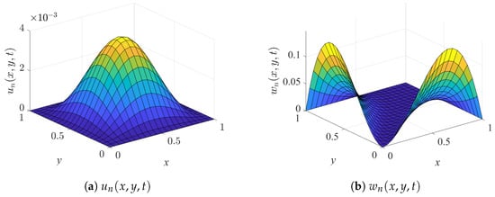
Figure 3. Numerical solutions (First Case).

Figure 4 illustrates the error distributions between the numerical and exact solutions. As shown in Figure 4, within the spatial domain $[0,1]\times [0,1]$, the absolute error $e_1(x,y,t)$ of $u(x,y,t)$ is less than $2\times {10}^{-13}$, while the absolute error $e_2(x,y,t)$ of $w(x,y,t)$ is less than $6\times {10}^{-12}$. Moreover, the corresponding relative errors are bounded by $3\times {10}^{-9}$ and $6\times {10}^{-10}$, respectively. These results indicate that the proposed Legendre polynomial algorithm achieves extremely high accuracy. The consistency between absolute and relative errors further demonstrates not only the precision of the approximation but also the numerical robustness of the method in this test case.

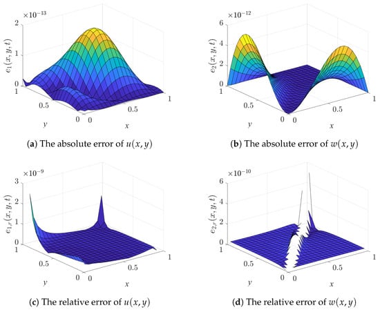
Figure 4. The absolute and relative error distributions (First Case).

6.2. Second Case

The boundary and of this example are shown as follows:

$$\begin{array}{c}\hfill u(x,0,t)=w(x,0,t)=u(x,1,t)=w(x,1,t)=0.\end{array}$$

(81)

The initial conditions are set as follows:

$$\begin{array}{c}\hfill {\displaystyle \frac{\partial u(x,y,0)}{\partial t}}={\displaystyle \frac{\partial w(x,y,0)}{\partial t}}=0.\end{array}$$

(82)

Similarly, based on the boundary and initial conditions, an exact example can be manufactured as follows:

$$\left\{\begin{array}{cc}\hfill u(x,y,t)& =-(x·(x-0.5)·(x-1)·(1-y)+x·(x-0.5)·(1-x)·y)·t^2;\hfill \\ \hfill w(x,y,t)& =t^2·(6·{(x-0.5)}^2-1.5).\hfill \end{array}\right.$$

(83)

After substituting parameters shown in Table 2, as well as Equation (83) into Equations (10) and (11), $F_z$ and $F_r$ can be obtained as follows:

$$\begin{array}{cc}\hfill F_z(x,y,t)=& 10{\displaystyle \frac{t^{1.1}}{1.05}}\left[x(x-1)+x(x-0.5)+x(x-1)(x-0.5)\right]+2.4t^2+t^2\left[(x-1)(x-0.5)+x(x-1)+x(x-0.5)\right]\hfill \\ \hfill & -0.05\left[2x(x-1)(x-0.5)(y-1)+2xy(x-1)(x-0.5)\right]+t^2(x-1)(x-0.5)-{\displaystyle \frac{-0.4t^2(12x-6)}{2x}}\hfill \\ \hfill & +24{\displaystyle \frac{t^{1.1}}{1.05}}+10{\displaystyle \frac{t^{1.1}(x-1)(x-0.5)}{1.05}}+2{\displaystyle \frac{-0.4t^{1.1}(12x-6)}{1.05x}};\hfill \end{array}$$

(84)

$$\begin{array}{cc}\hfill F_r(x,y,t)=& -0.7x^2{t}^2\left[x(x-1)(x-0.5)(y-1)+xy(x-1)(x-0.5)\right]+0.7t^2\left[2(x-1)(y-1)+2(x-0.5)(y-1)+2y(x-0.5)\right]\hfill \\ \hfill & +0.7{\displaystyle \frac{t^2}{x}}\left[xy(x-1)+xy(x-0.5)+x(x-1)(y-1)+x(x-0.5)(y-1)+y(x-1)(x-0.5)+(x-1)(x-0.5)(y-1)\right]\hfill \\ \hfill & -0.05\left[2x(x-1)(x-0.5)(y-1)+2xy(x-1)(x-0.5)\right]+{\displaystyle \frac{7t^{1.1}}{1.05}}\left[2(x-1)(y-1)+2(x-0.5)(y-1)+2y(x-0.5)\right]\hfill \\ \hfill & -{\displaystyle \frac{7t^{1.1}}{1.05x^2}}\left[x(x-1)(x-0.5)(y-1)+xy(x-1)(x-0.5)\right]+{\displaystyle \frac{7t^{1.1}}{1.05x^2}}\left[xy(x-1)+xy(x-0.5)+(x-1)(x-0.5)(y-1)\right].\hfill \end{array}$$

(85)

Then, substituting parameters shown in Table 2, as well as Equations (84) and (85) in to Equations (10) and (11), the governing equations are obtained as follows:

$$\{\begin{array}{}\mathrm{(86)}& \begin{array}{cc}& \frac{7}{10}{\displaystyle \frac{{\partial }^{2}u}{\partial y^2}}+\frac{1}{5}{\displaystyle \frac{{\partial }^{2}u}{\partial x^2}}+\frac{1}{2}{\displaystyle \frac{{\partial }^{2}w}{\partial y\partial x}}+\frac{7}{10y}{\displaystyle \frac{\partial u}{\partial y}}-\frac{7}{10y^2}u+\frac{7}{2}{D}^{0.9}\left({\displaystyle \frac{{\partial }^{2}u}{\partial y^2}}\right)\hfill \\ & +D^{0.9}\left({\displaystyle \frac{{\partial }^{2}u}{\partial x^2}}\right)+\frac{5}{2}{D}^{0.9}\left({\displaystyle \frac{{\partial }^{2}w}{\partial y\partial x}}\right)+\frac{7}{2y}{D}^{0.9}\left({\displaystyle \frac{\partial u}{\partial y}}\right)-\frac{7}{2y^2}{D}^{0.9}\left(u\right)+F_r-\frac{13}{525}{\displaystyle \frac{{\partial }^{2}u}{\partial t^2}}=0\hfill \end{array}\mathrm{(87)}& \begin{array}{cc}& \frac{1}{5}{\displaystyle \frac{{\partial }^{2}w}{\partial y^2}}+\frac{7}{10}{\displaystyle \frac{{\partial }^{2}w}{\partial x^2}}+\frac{1}{2}{\displaystyle \frac{{\partial }^{2}u}{\partial y\partial x}}+\frac{1}{5y}{\displaystyle \frac{\partial w}{\partial y}}+\frac{1}{2y}{\displaystyle \frac{\partial u}{\partial x}}+D^{0.9}\left({\displaystyle \frac{{\partial }^{2}w}{\partial y^2}}\right)\hfill \\ & +\frac{7}{2}{D}^{0.9}\left({\displaystyle \frac{{\partial }^{2}w}{\partial x^2}}\right)+\frac{5}{2}{D}^{0.9}\left({\displaystyle \frac{{\partial }^{2}u}{\partial y\partial x}}\right)+\frac{1}{r}{D}^{0.9}\left({\displaystyle \frac{\partial w}{\partial y}}\right)+\frac{5}{2y}{D}^{0.9}\left({\displaystyle \frac{\partial u}{\partial x}}\right)-\frac{13}{525}{\displaystyle \frac{{\partial }^{2}w}{\partial t^2}}+F_z=0\hfill \end{array}\hfill \end{array}$$

Table 2. Parameters of Second Case.

E	$\mathit{\rho }$	$\mathit{\nu }$	$\mathit{\delta }$	${\mathit{\tau }}_{\mathit{\sigma }}^{\mathit{E}}$	H	R
${\displaystyle \frac{525}{13}}$	1	$0.3$	$0.9$	$5.975$	1	1

When $n_1=n_2=n_3=4$ and $t=1$, the system of equations is solved using the Legendre polynomial algorithm. Figure 5 and Figure 6 present the computed results of $u(x,y,t)$ and $w(x,y,t)$, including both the exact and numerical solutions. Here, $u(x,y,t),w(x,y,t)$ denote the exact solutions, while $u_n(x,y,t),w_n(x,y,t)$ are the numerical solutions. To further evaluate the accuracy, both the absolute errors $e_1(x,y,t),e_2(x,y,t)$ and the relative errors $e_{1,r}(x,y,t),e_{2,r}(x,y,t)$ are considered, with their distributions illustrated in Figure 7. These errors are defined as

$$\begin{array}{cccc}\hfill e_1(x,y,t)& =|u(x,y,t)-u_n(x,y,t)|,\hfill & \hfill e_2(x,y,t)& =|w(x,y,t)-w_n(x,y,t)|,\hfill \\ \hfill e_{1,r}(x,y,t)& ={\displaystyle \frac{|u(x,y,t)-u_n(x,y,t)|}{\left|u\right(x,y,t\left)\right|}},\hfill & \hfill e_{2,r}(x,y,t)& ={\displaystyle \frac{|w(x,y,t)-w_n(x,y,t)|}{\left|w\right(x,y,t\left)\right|}}.\hfill \end{array}$$

(88)

When computing the relative errors, grid points at which the exact solution $u(x,y,t)$ or $w(x,y,t)$ is smaller than a prescribed tolerance $\epsilon ={10}^{-12}$ are excluded to avoid division by zero and artificial amplification of the error.

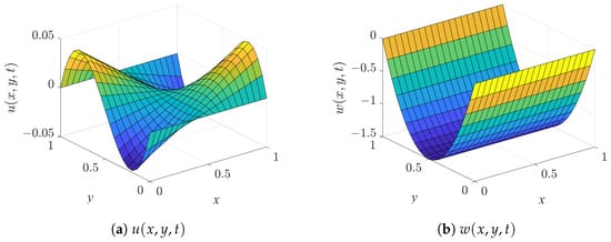
Figure 5. Exact Solutions (Second Case).

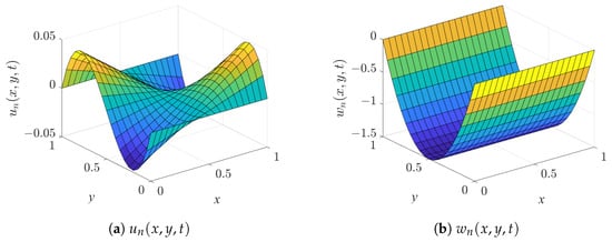
Figure 6. Numerical Solutions (Second Case).

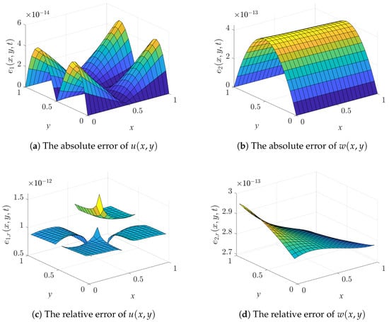
Figure 7. The absolute and relative error distributions (Second Case).

As shown in Figure 7, the absolute and relative errors are both confined to extremely small ranges. Specifically, for $u(x,y,t)$ the absolute error $e_1(x,y,t)$ is less than $6\times {10}^{-14}$ and the relative error $e_{1,r}(x,y,t)$ is less than $2\times {10}^{-12}$, while for $w(x,y,t)$ the absolute error $e_2(x,y,t)$ is less than $5\times {10}^{-13}$ and the relative error $e_{2,r}(x,y,t)$ is less than $3\times {10}^{-13}$. These results demonstrate not only the high accuracy of the proposed algorithm but also its numerical stability and reliability in this test case.

By solving the numerical equations under fixed (homogeneous Dirichlet) boundary conditions and validating them against exact solutions, the proposed method has been shown to achieve very high accuracy and stable convergence. These results confirm both the feasibility and reliability of the approach under fixed constraints. As a next step, practical case studies will be incorporated to further illustrate the effectiveness and engineering relevance of the method. Moreover, the extension of the present framework to other boundary conditions, such as free and simply supported cases, is conceptually straightforward and will be pursued in future work.

7. Dynamic Analysis of Fractional-Order Viscoelastic Spinning Disks

In the previous section, the accuracy and convergence of the proposed algorithm were verified through benchmark tests. And in this section, to verify the effectiveness and applicability of the proposed method in practical applications, numerical simulations were conducted on a specific disk model. The geometric parameters and material properties of the disk model were kept constant, as shown in Table 3. The density of a body force $F_z$ and rotational speed $\omega$ were treated as the primary control variables. By varying these two parameters, their effects on the dynamic response of the disk were analyzed. In this model, the boundary conditions are set as follows:

$$\begin{array}{c}\hfill u(x,0,t)=w(x,0,t)=u(x,0.4,t)=w(x,0.4,t)=0;\end{array}$$

(89)

Table 3. Geometric and material parameters of spinning disk.

Parameter	Notation	Value
Young’s modulus	E (GPa)	110
Density	$\rho$ (${\mathrm{kg}/\mathrm{m}}^3$)	7800
Poisson’s ratio	$\nu$	0.05
Fractional derivative order	$\delta$	0.66
Retardation time	${\tau }_{\sigma }^E$(s)	0.0107
Thickness	H (m)	0.2
Radius	R (m)	0.4

The initial conditions are

$$\begin{array}{c}\hfill {\displaystyle \frac{\partial u(x,y,0)}{\partial t}}={\displaystyle \frac{\partial w(x,y,0)}{\partial t}}=0.\end{array}$$

(90)

In the numerical experiments, most of the results are presented at $t=1$ for clarity. In addition, a representative earlier time $t=0.1$ is also considered. The choice of $t=0.1$ does not have a particular physical meaning, but it avoids the trivial zero solution at the initial instant and provides a meaningful snapshot for numerical verification. Furthermore, to complement the spatial distributions, the displacement evolution at a representative spatial point with respect to time is also investigated, which further demonstrates the temporal accuracy and stability of the proposed algorithm.

7.1. Effect of Different Rotational Speeds on Radial Displacement

The Legendre polynomial algorithm was used to solve the equations. When $n_1=n_2=n_3=4$, $t=1$ s and $P=212.75$ MPa, some results for the radial displacement can be obtained, as shown in Figure 8. When a constant transverse body force density is applied to the disk and the disk begins to rotate, the disk undergoes deformation and experiences both transverse and radial displacements. Figure 8 demonstrates that when $y=0$ m and $y=0.4$ m, the radial displacement u are zero, which satisfies the boundary conditions. When $\omega =5.4$ RPM, the radial deformation is shown in Figure 8a. It also shows that the maximum radial displacement is $0.611$ m, occurring at $x=0\mathrm{m}$, $y=0.08\mathrm{m}$. The radial displacement is symmetric about $x=0.1\mathrm{m}$, $y=0.2\mathrm{m}$. Additionally, under different rotational speeds, the variation of radial displacement of the disk is also investigated. Figure 8 also illustrates the variation in radial displacement distribution with respect to the different rotational speed $\omega$. Under the same body force density and time conditions, the differences in radial displacement of the disk exhibit different trends. Quantitatively, the peak displacement increases monotonically with $\omega$: from $0.375$ m at $\omega =0.3$ RPM, to $0.551$ m at $\omega =3.1$ RPM, and $0.611$ m at $\omega =5.4$ RPM, corresponding to an overall amplification of about $63\%$. As the rotational speed $\omega$ increases, the area with large displacement becomes wider, and the peak displacement region grows more obvious, showing a clear strengthening of the deformation trend. As shown in Figure 8, with an increase in rotational speed, the maximum radial displacement also increases correspondingly, and the distribution range of the radial displacement expands. Specifically, when $\omega$ values $0.3$ RPM, $3.1$ RPM, and $5.4$ RPM, the maximum radial displacements are $0.375$ m, $0.551$ m and $0.61$ m, respectively. From an engineering perspective, these results imply that higher rotational speeds significantly amplify in-plane deformation, which must be considered in stiffness design and tolerance evaluation of spinning disks.

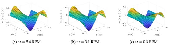
Figure 8. Radial Displacement Distribution ($F_z=212.75$ MPa).

7.2. Effect of Varying Body Force Density on Transverse Displacement

Under different body force density, the transverse displacement variations of the disk are investigated. When $n_1=n_2=n_3=4$, $t=1$ s and $\omega =5.4$ RPM, the transverse displacement distributions are shown in Figure 9. It demonstrates that when $y=0$ m and $y=0.4$ m, the transverse displacements w are zero, which satisfies the boundary conditions. When $F_z=212.75$ MPa, the transverse displacement distributions are shown in Figure 9a. It shows that the maximum transverse displacement is $2.13$ m, occurring at $x=0.16$ m, $y=0.2$ m. The transverse displacement is axisymmetric with respect to $y=0.2$ m. Figure 9 illustrates the variation in transverse displacement distribution with respect to the density of a body force $F_z$. Under the same rotational speed and time conditions, as the body force density increases, the transverse displacement exhibits different trends. Figure 9 shows that as the body force density increases, the maximum transverse displacement also increases correspondingly, and the distribution range of the displacement expands. Quantitatively, the peak values are $1.04$ m, $1.86$ m, and $2.13$ m for $F_z=72.5$ MPa, $147.5$ MPa, and $212.75$ MPa, respectively, corresponding to an overall amplification of about $2.13/1.04\approx 2.05$ (i.e., ∼105% increase). As $F_z$ grows, the area with large $\left|w\right|$ visibly expands and the trough near the center becomes more pronounced, showing a clearer deformation pattern while remaining consistent with the boundary constraints. When $F_z$ values $72.5$ MPa, $147.5$ MPa, and $212.75$ MPa, the maximum transverse displacements are $1.04$ m, $1.86$ m and $2.13$ m, respectively. Specifically, larger body force density cause more significant transverse deformation, which is particularly pronounced in the central region of the disk. From an engineering viewpoint, higher body force density significantly magnifies the out-of-plane deflection under the same rotation, which should be considered in stiffness sizing and allowable-deflection criteria for spinning disks. The distribution characteristics and variation in the maximum values of transverse displacement under different body force density conditions reflect the impact of the body force density on the disk deformation.

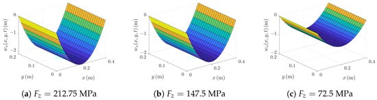
Figure 9. Transverse Displacement Distribution ($\omega =5.4$ RPM).

7.3. Temporal Response at a Representative Point

To assess the numerical stability and accuracy of the proposed algorithm in the time direction, we examine the temporal evolution of $u_n$ and $w_n$ at the representative spatial point $(x,y)=(0.05,0.1)$. The computational settings are a rotational speed $\omega =5.4$ RPM and a body force density parameter $F_z=25$ MPA; the remaining geometric and material parameters are identical to those in Table 3. In Figure 10, the displacement response at the point $(x,y)=(0.05,0.1)$ is plotted over the time interval $t\in [0,0.8]$.

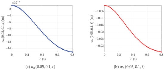
Figure 10. Displacement response at $(x,y)=(0.05,0.1)$ over time.

As shown in Figure 10, both $u_n(0.05,0.1,t)$ and $w_n(0.05,0.1,t)$ vary monotonically with time. The curves are overall concave downward. In the initial stage, the increase (in absolute value) is relatively rapid. Subsequently, the growth rate gradually decreases. This behavior exhibits the typical “creep-like” slow evolution of fractional viscoelastic systems. The two curves are smooth and continuous without numerical oscillations or noise, indicating good numerical stability of the time marching and the treatment of history terms under this operating condition. Meanwhile, the magnitude of $w_n$ is significantly larger than that of $u_n$, implying that, under the present loading and boundary conditions, the disk’s deformation is primarily governed by bending, with in-plane deformation contributing only marginally. In summary, the time histories at this representative point further corroborate the accuracy and stability of the algorithm in the time direction. Consistent with the previously reported spatial-distribution errors (absolute and relative), the displacement variation over time provides additional evidence for the method’s applicability in engineering contexts.

8. Conclusions

This paper investigates the viscoelastic spinning disk based on the fractional-order Kelvin–Voigt model and employs the shifted Legendre polynomial algorithm to solve the nonlinear system of differential equations. Verification results show that the algorithm provides high accuracy and low complexity in solving such systems. And this algorithm has demonstrated great potential for application in solving higher-dimensional and more complex problems. The following conclusions are drawn from the analysis:

• The shifted Legendre polynomial algorithm accurately captures the radial and transverse displacements of the viscoelastic spinning disk in the time domain, with both absolute and relative errors reaching very small magnitudes. This highlights the method’s numerical stability and robustness.
• A comparison and analysis of the radial and transverse displacements of the viscoelastic spinning disk under different rotational speeds and body force density are presented. The results confirm that increasing rotational speed and body force density significantly enlarges the displacement field, which has direct engineering implications for stiffness design and safety margins.
• Based on convergence analysis and numerical examples, it is demonstrated that the proposed method achieves high precision in solving the fractional-order partial differential equations of the viscoelastic spinning disk control equations under different boundary conditions. The methodology is general and can be extended to other fractional viscoelastic structures such as plates and sandwich composites.

References

- Peng, Y.; Zhao, J.; Li, Y. A wellbore creep model based on the fractional viscoelastic constitutive equation. Pet. Explor. Dev. 2017, 44, 1038–1044. [Google Scholar] [CrossRef]
- Sun, H.; Zhang, Y.; Baleanu, D.; Chen, W.; Chen, Y. A new collection of real world applications of fractional calculus in science and engineering. Commun. Nonlinear Sci. Numer. Simul. 2018, 64, 213–231. [Google Scholar] [CrossRef]
- Lewandowski, R.; Chorążyczewski, B. Identification of the parameters of the Kelvin–Voigt and the Maxwell fractional models, used to modeling of viscoelastic dampers. Comput. Struct. 2010, 88, 1–17. [Google Scholar] [CrossRef]
- Kim, S.; Lee, D. Identification of fractional-derivative-model parameters of viscoelastic materials from measured FRFs. J. Sound Vib. 2009, 324, 570–586. [Google Scholar] [CrossRef]
- Zhao, X.; Yang, H.; He, Y. Identification of constitutive parameters for fractional viscoelasticity. Commun. Nonlinear Sci. Numer. Simul. 2014, 19, 311–322. [Google Scholar] [CrossRef]
- Shi, Z.; Zhou, J.; Song, D.; Cui, J.; Yuan, M.; Miao, C. The viscoelastic stress wave propagation model based on fractional derivative constitutive. Int. J. Impact Eng. 2025, 202, 105330. [Google Scholar] [CrossRef]
- Tang, K.; Wen, M.; Ding, P.; Zhang, Y.; Tu, Y.; Xie, J.; Liu, K.; Wu, D. Fractional derivative modelling for consolidation of multilayered saturated soils with interfacial thermal contact resistance subjected to time-dependent heating and loading. Geomech. Energy Environ. 2024, 38, 100553. [Google Scholar] [CrossRef]
- Mohammad, N.; Alsalmi, A.R.; Awad, N.; Ma, Y.; Saranya, S.; Al-Mdallal, Q. Application of fractional derivative in Buongiorno’s model for enhanced fluid flow and heat transfer analysis over a permeable cylinder. Int. J. Thermofluids 2025, 26, 101129. [Google Scholar] [CrossRef]
- Zheng, G.; Zhang, N.; Lv, S. The Application of Fractional Derivative Viscoelastic Models in the Finite Element Method: Taking Several Common Models as Examples. Fractal Fract. 2024, 8, 103. [Google Scholar] [CrossRef]
- Geetanjali, G.; Sharma, P.K. Vibrational analysis of transversely isotropic hollow cylinder based on fractional generalized thermoelastic diffusion models with nonlocal effects. Acta Mech. 2024, 235, 147–166. [Google Scholar] [CrossRef]
- Permoon, M.R.; Haddadpour, H.; Shakouri, M. Nonlinear vibration analysis of fractional viscoelastic cylindrical shells. Acta Mech. 2020, 231, 4683–4700. [Google Scholar] [CrossRef]
- Alitasb, G.K. Assessment of Fractional and Integer Order Models of Induction Motor Using MATLAB/Simulink. Mod. Simul. Eng. 2024, 2024, 2739649. [Google Scholar] [CrossRef]
- Cortés, F.; Brun, M.; Elejabarrieta, M.J. A finite element formulation for the transient response of free layer damping plates including fractional derivatives. Comput. Struct. 2023, 282, 107039. [Google Scholar] [CrossRef]
- Sun, L.; Qu, J.; Cheng, G.; Barrière, T.; Cui, Y.; Yang, A.; Chen, Y. Numerical analysis for variable thickness plate with variable order fractional viscoelastic model. Commun. Nonlinear Sci. Numer. Simul. 2025, 146, 108764. [Google Scholar] [CrossRef]
- Zhang, M.; Hao, Y.; Chen, Y.; Cheng, G.; Barrière, T.; Qu, J. Modeling and dynamic analysis of fractional order nonlinear viscoelastic rod. Int. J. Non-Linear Mech. 2024, 162, 104699. [Google Scholar] [CrossRef]
- Hao, Y.; Zhang, M.; Cui, Y.; Cheng, G.; Xie, J.; Chen, Y. Dynamic analysis of variable fractional order cantilever beam based on shifted Legendre polynomials algorithm. J. Comput. Appl. Math. 2023, 423, 114952. [Google Scholar] [CrossRef]
- Salehi, M.; Aghaei, H. Dynamic relaxation large deflection analysis of non-axisymmetric circular viscoelastic plates. Comput. Struct. 2005, 83, 1878–1890. [Google Scholar] [CrossRef]
- Shariyat, M.; Mohammadjani, R. Three-Dimensional Dynamic Stress and Vibration Analyses of Thick Singular-Kernel Fractional-Order Viscoelastic Annular Rotating Discs Under Nonuniform Loads. Int. J. Struct. Stab. Dyn. 2020, 20, 2050007. [Google Scholar] [CrossRef]
- Heydari, M.; Atangana, A.; Avazzadeh, Z. Numerical solution of nonlinear fractal-fractional optimal control problems by Legendre polynomials. Appl. Math. Lett. 2020, 107, 106443. [Google Scholar] [CrossRef]
- Dahaghin, M.; Hassani, H.S. An optimization method based on the generalized polynomials for nonlinear variable-order time fractional diffusion-wave equation. Nonlinear Dyn. 2017, 88, 1587–1598. [Google Scholar] [CrossRef]
- Cao, J.; Chen, Y.; Wang, Y.; Cheng, G.; Barrière, T. Shifted Legendre polynomials algorithm used for the dynamic analysis of PMMA viscoelastic beam with an improved fractional model. Chaos Solitons Fractals 2020, 141, 110342. [Google Scholar] [CrossRef]
- Wang, L.; Chen, Y.; Cheng, G.; Barrière, T. Numerical analysis of fractional partial differential equations applied to polymeric visco-elastic Euler-Bernoulli beam under quasi-static loads. Chaos Solitons Fractals 2020, 140, 110255. [Google Scholar] [CrossRef]
- Dang, R.; Yang, A.; Chen, Y.; Wei, Y.; Yu, C. Vibration analysis of variable fractional viscoelastic plate based on shifted Chebyshev wavelets algorithm. Comput. Math. Appl. 2022, 119, 149–158. [Google Scholar] [CrossRef]
- Sun, L.; Chen, Y. Numerical analysis of variable fractional viscoelastic column based on two-dimensional Legendre wavelets algorithm. Chaos Solitons Fractals 2021, 12, 111372. [Google Scholar] [CrossRef]
- Chen, Y.; Sun, Y.; Liu, L. Numerical solution of fractional partial differential equations with variable coefficients using generalized fractional-order Legendre functions. Appl. Math. Comput. 2014, 244, 847–858. [Google Scholar] [CrossRef]
- Taghvafard, H.; Erjaee, G. Phase and anti-phase synchronization of fractional order chaotic systems via active control. Commun. Nonlinear Sci. Numer. Simul. 2011, 16, 4079–4088. [Google Scholar] [CrossRef]
- Yi, M.; Wang, L.; Huang, J. Legendre wavelets method for the numerical solution of fractional integro-differential equations with weakly singular kernel. Appl. Math. Model. 2016, 40, 3422–3437. [Google Scholar] [CrossRef]
- Li, C.; Qian, D.; Chen, Y. On Riemann-Liouville and Caputo Derivatives. Discret. Dyn. Nat. Soc. 2011, 2011, 562494. [Google Scholar] [CrossRef]
- Pritz, T. Analysis of four-parameter fractional derivative model of real solid materials. J. Sound Vib. 1996, 195, 103–115. [Google Scholar] [CrossRef]
- Xu, H.; Jiang, X. Creep constitutive models for viscoelastic materials based on fractional derivatives. Comput. Math. Appl. 2017, 73, 1377–1384. [Google Scholar] [CrossRef]
- Shen, M.; Chen, S.; Liu, F. Unsteady MHD flow and heat transfer of fractional Maxwell viscoelastic nanofluid with Cattaneo heat flux and different particle shapes. Chin. J. Phys. 2018, 56, 1199–1211. [Google Scholar] [CrossRef]
- Ren, D.; Shen, X.; Li, C.; Cao, X. The fractional Kelvin–Voigt model for Rayleigh surface waves in viscoelastic FGM infinite half space. Mech. Res. Commun. 2018, 87, 53–58. [Google Scholar] [CrossRef]
- Farno, E.; Baudez, J.; Eshtiaghi, N. Comparison between classical Kelvin–Voigt and fractional derivative Kelvin–Voigt models in prediction of linear viscoelastic behaviour of waste activated sludge. Sci. Total Environ. 2018, 613–614, 1031–1036. [Google Scholar] [CrossRef]
- Pawlus, D. Three-Layered Annular Plate Made of Functionally Graded Material Under a Static Temperature Field. Materials 2024, 17, 5484. [Google Scholar] [CrossRef]
- Ciarlet, P.G. The Finite Element Method for Elliptic Problems; Classics in Applied Mathematics; SIAM: Philadelphia, PA, USA, 2002; Volume 40. [Google Scholar] [CrossRef]
- Canuto, C.; Hussaini, M.Y.; Quarteroni, A.; Zang, T.A. Spectral Methods: Fundamentals in Single Domains; Scientific Computation; Springer: Berlin/Heidelberg, Germany, 2006. [Google Scholar] [CrossRef]
- Zayernouri, M.; Karniadakis, G.E. Fractional spectral collocation methods for linear and nonlinear variable order FPDEs. J. Comput. Phys. 2015, 293, 312–338. [Google Scholar] [CrossRef]
- Saadatmandi, A.; Dehghan, M. A new operational matrix for solving fractional-order differential equations. Comput. Math. Appl. 2010, 59, 1326–1336. [Google Scholar] [CrossRef]
- Wang, Y.; Chen, Y. Shifted Legendre Polynomials algorithm used for the dynamic analysis of viscoelastic pipes conveying fluid with variable fractional order model. Appl. Math. Model. 2020, 81, 159–176. [Google Scholar] [CrossRef]
- Li, C.; Zhang, Y.; Jia, Y.; Chen, J. The polygonal scaled boundary thin plate element based on the discrete Kirchhoff theory. Comput. Math. Appl. 2021, 97, 223–236. [Google Scholar] [CrossRef]
Disclaimer/Publisher’s Note: The statements, opinions and data contained in all publications are solely those of the individual author(s) and contributor(s) and not of MDPI and/or the editor(s). MDPI and/or the editor(s) disclaim responsibility for any injury to people or property resulting from any ideas, methods, instructions or products referred to in the content. |
© 2025 by the authors. Licensee MDPI, Basel, Switzerland. This article is an open access article distributed under the terms and conditions of the Creative Commons Attribution (CC BY) license (https://creativecommons.org/licenses/by/4.0/).