Efficient Scheme for Solving Tempered Fractional Quantum Differential Problem

Abstract

This study presents a novel family of operators, referred to as tempered quantum fractional operators, and investigates the well-posedness of related tempered quantum fractional differential equations. The q-Adams predictor–corrector method is employed to conduct the analysis. By carefully adjusting the scheme’s parameters, the convergence rate can be controlled, while computational expenses increase linearly with time. Numerical simulations confirm the effectiveness and precision of the introduced algorithm.

1. Introduction

The mathematical framework of q-calculus (quantum calculus) was formalized in several classical works that established the algebraic and analytic basics of the subject. Foundational expositions on quantum calculus and its algebraic structures are presented in [1,2,3]. The fractional extension of quantum calculus, introducing fractional quantum derivatives and their integral representations, was developed and popularized by Ortigueira [4] and related authors. Early investigations connecting q-difference equations to quantum-symmetric structures and orthogonal polynomials appear in studies such as Floreanini and Vinet [5] and Freund and Zabrodin [6], which highlighted spectral and symmetry aspects of q-difference problems. Applications of q-difference techniques to continuum mechanics and material models (e.g., microstretch thermoelasticity) were explored by Marin [7]. Recent contributions have focused on q-fractional operators, their analytic properties, and numerical methods. Sadek and Algefary introduced a quantum trigonometric fractional calculus and provided concrete analytical examples in [8]. Existence and boundary-value theory for fractional q-difference equations with nonlocal conditions were treated by Zhao et al. [9], while Abdeljawad, Benli, and Baleanu developed generalized q-Mittag–Leffler constructions for q-Caputo equations [10].

Methodological advances for solving q-fractional equations numerically and analytically have been proposed by Koca [11]. Further numerical remarks and corrections concerning q-fractional formulations were examined by Tang and Zhang [12] and by Noeiaghdam et al. in contexts involving uncertainty [13]. Solution theory and well-posedness for nonlinear q-fractional problems were developed more recently by Zhang and Guo [14], providing rigorous frameworks for existence and uniqueness. Efficient numerical schemes tailored to q-fractional models were proposed in [15] and extended in [16] to improve stability and convergence. Complementary theoretical foundations for fractional operators (not restricted to the q-setting) that inform kernel choice, tempering, and Caputo-type modifications are provided in [17,18,19]. These works supply general operator properties and motivations used when defining tempered or modified fractional derivatives. Several recent works by the present authors and close collaborators introduced specialized fractional operators, numerical algorithms, and applications relevant to the present study; see [20,21]. These contributions motivated the tempered and trigonometric extensions treated here and provided prototypes for numerical experimentation and stability analysis.

For physical motivation and empirical grounding, anomalous diffusion modeling and single-particle tracking literature summarize key phenomena that tempered fractional models aim to capture; see Metzler et al. [22]. The notion of tempering and finite-memory corrections is also supported by classical fractional literature [18,19]. Collecting these developments, the literature shows (i) a solid algebraic and analytic base for q-calculus [1,2,3], (ii) established fractional and generalized fractional constructions including q-extensions [4,10,23], and (iii) growing work on numerical schemes and applications [11,15,16]. Motivated by these strands, the present paper introduces a family of tempered quantum fractional (Caputo-type) operators, establishes well-posedness results, and proposes a q-Adams predictor–corrector numerical scheme with controlled convergence and linear computational complexity.

To the best of our knowledge, the investigation of q-$\mathbb{FDE}$s incorporating trigonometric derivatives represents an unexplored research direction in fractional calculus. This work addresses this gap by introducing novel trigonometric q-integral and q-derivative operators. We establish their fundamental definitions and rigorously characterize their mathematical properties, creating a systematic framework for theoretical analysis and applications.

Physical Motivation and Potential Applications. While the mathematical framework of q-fractional calculus is elegant in its own right, it also finds compelling physical interpretations and potential applications. The parameter q inherently introduces a discrete or multi-scale structure, making q-calculus a natural tool for modeling phenomena on hierarchical lattices, in fractal media, or within systems with discrete energy levels, such as quantum dots and non-uniform quantum wells [1]. In such contexts, the standard continuum models may fail to capture the essential physics. The introduction of tempered fractional operators, via the parameter $\lambda \ge 0$, further enriches this modeling capability. Tempering introduces an exponential cut-off to the power-law memory kernel characteristic of fractional derivatives. Physically, this can represent a finite lifespan of memory effects, a transition from anomalous to normal diffusion at long timescales, or a truncation of long-range interactions [18]. For instance, the tempered q-fractional derivative developed in this work could describe anomalous charge carrier relaxation in a discrete quantum system where memory effects are significant initially but decay exponentially over time, we now mention:

• Tempered Diffusion on q-Lattices: The parameter q can model discrete, hierarchical, or fractal structures where standard continuum models fail. The tempered operator, with its exponential kernel, can describe processes where anomalous diffusion (captured by $\alpha$) transitions to classical behavior over longer timescales (captured by $\lambda$).
• Non-Uniform Quantum Wells: The q-calculus framework is naturally suited for systems with discrete spatial coordinates or energy levels, such as quantum dots or finite-difference models of heterostructures. The tempered fractional derivative could model memory effects in charge carrier relaxation in such systems.

Modern Practical Applications. The development of tempered quantum fractional operators is motivated by several emerging challenges in modern science and engineering where conventional models prove inadequate. Specific practical scenarios that could benefit from this framework include:

• Transport in Nanostructured and Porous Materials: Materials such as nanoporous silica, aerogels, and catalytic substrates exhibit complex multi-scale geometries that can be naturally described by q-calculus. Charge and mass transport in these materials often shows anomalous diffusion (captured by $\alpha$) due to trapping and disordered pathways, while the tempering parameter $\lambda$ can model the finite size effects and crossover to normal diffusion at larger scales. Our operators provide a unified tool to model such complex transport phenomena.
• Dynamics in Quantum Technologies: In quantum computing architectures and quantum dot arrays, the discrete nature of energy levels and spatial arrangements aligns naturally with q-calculus. The tempered fractional framework can describe memory effects in qubit decoherence or charge relaxation processes where quantum correlations have finite lifetimes, offering more accurate models for quantum device performance and reliability.
• Control of Fractional-Order Discrete Systems: Modern control applications involving networked systems, digital controllers, and multi-agent systems often operate on discrete time scales. The tempered q-fractional operators enable the development of sophisticated control strategies that account for memory effects with finite temporal correlations, potentially leading to more robust and efficient control algorithms for complex technological systems.

These applications demonstrate that tempered quantum fractional operators address a genuine need in contemporary research, bridging the gap between abstract mathematical formalism and pressing technological challenges.

Therefore, the synthesis of q-calculus, fractional operators, and tempering creates a powerful and flexible mathematical tool for modeling complex dynamics in structured and multi-scale physical systems.

A key innovation of this study is the development of a trigonometric Caputo-type q-derivative operator and its associated q-integral, significantly enriching the mathematical apparatus for solving complex problems. Furthermore, we propose a q-analogue of the Laplace transform as an effective analytical method for q-dynamical systems. The practical applicability of our framework is demonstrated through comprehensive solutions of two representative examples.

Our research contributes to advancing fractional calculus by developing new theoretical constructs within the q-fractional paradigm. The synthesis of q-calculus, fractional operators, and trigonometric differentiation offers researchers both theoretical insights and computational tools for modeling sophisticated dynamical systems.

In the present study, we develop a novel numerical scheme for analyzing and solving nonlinear q-$\mathbb{FDE}$s of the form:

$$\left\{\begin{array}{cc}{}_a{}^{\mathrm{C}}\nabla _{\mathfrak{r}}^{\alpha ,\lambda ,q}x\left(\mathfrak{r}\right)=\sigma (\mathfrak{r},x\left(\mathfrak{r}\right)),\hfill & a\in {\mathbb{T}}_q,0<q<1,\hfill \\ {\nabla }_q^k{\left[e_q^{\lambda \mathfrak{r}}x\left(\mathfrak{r}\right)\right]}_{\mathfrak{r}=a}=x_0^{\left(k\right)}\in \mathbb{R},\hfill & k=0,1,\dots ,\left[\alpha \right]-1,\hfill \end{array}\right.$$

(1)

where ${}_a{}^{\mathrm{C}}\nabla _{\mathfrak{r}}^{\alpha ,\lambda ,q}x\left(\mathfrak{r}\right)$ denotes tempered quantum fractional derivative of Caputo type, and $\sigma :{\mathbb{T}}_q\times \mathbb{R}⟶\mathbb{R}$ is function.

In the following sections, we first introduce fundamental concepts of q-calculus (q-C) and q-fractional calculus in Section 3. Subsequently, in Section 5, we examine q-ordinary differential equations (q-$\mathbb{ODE}$s) involving both Riemann-Liouville (RL) and Caputo-type tempered q-fractional derivatives. Under appropriate conditions, we reformulate the Cauchy problem (1) as second-kind q-Volterra integral equations (q-$\mathbb{VIE}$s).

Notational Conventions:

Throughout this work, we employ the following standardized terminology:

• q-$\mathbb{FDE}$s: Quantum fractional differential equations (general term)
• q-$\mathbb{OFDE}$s: Quantum ordinary fractional differential equations (when emphasizing the ordinary vs. partial distinction)
• q-$\mathbb{VIE}$s: Quantum Volterra integral equations (for the equivalent integral formulation)

The term “q-FIDE” is avoided to prevent confusion with fractional integro-differential equations.

2. Physical Case Study: Anomalous Diffusion in a Hierarchical Porous Medium

To demonstrate the physical relevance and advantages of the tempered quantum fractional calculus, we apply our formalism to model anomalous diffusion in a hierarchical or fractal-like porous medium, such as nanoporous silica, aerogels, or certain biological tissues [22]. These systems are characterized by multi-scale geometries where transport phenomena deviate significantly from classical Fickian diffusion.

2.1. Problem Formulation and Model Comparison

We consider the transport of a solute concentration $u(\mathbf{r},t)$ through a complex medium. Standard models often fail to capture the complete dynamics observed experimentally, particularly the early-time sub-diffusion and the long-time transition to normal diffusion.

• Classical Model (Fick’s Law):

  $${\displaystyle \frac{\partial u}{\partial t}}=D{\displaystyle \frac{{\partial }^{2}u}{\partial x^2}}$$
  This model fails to capture the power-law waiting times and trapping events common in disordered media.
• Standard Fractional Model (Time-Fractional Diffusion):

  $${}_0{}^{\mathrm{C}}\nabla _t^{\alpha }u=D{\displaystyle \frac{{\partial }^{2}u}{\partial x^2}},0<\alpha <1$$
  This model excellently describes sub-diffusive behavior (mean-square displacement $⟨x^2\left(t\right)⟩\sim t^{\alpha }$) but predicts an infinite velocity for the solute front and perpetual memory, which is unphysical over long timescales.
• Our Proposed Model (Tempered Quantum Fractional Diffusion): We propose the following equation to describe the concentration $x\left(\mathbf{r}\right)$ at a specific point in the medium:

  $$\left\{\begin{array}{c}{}_0{}^{\mathrm{C}}\nabla _{\mathbf{r}}^{\alpha ,\lambda ,q}x\left(\mathbf{r}\right)={\left(e_q^{\lambda \mathbf{r}}\right)}^{-1}F\left(\mathbf{r}\right),\hfill \\ x\left(0\right)=x_0,\hfill \end{array}\right.$$

  (2)

  where $F\left(\mathbf{r}\right)$ encapsulates diffusion and source terms, $\kappa$ is a generalized diffusivity constant, and the operator ${}_0{}^{\mathrm{C}}\nabla _{\mathbf{r}}^{\alpha ,\lambda ,q}$ simultaneously captures the discrete geometry, memory effects, and finite correlation lengths characteristic of hierarchical porous media.

2.2. Physical Interpretation of Parameters in Context

The parameters in our model directly correspond to physical properties of the porous medium:

• Quantum Parameter $\mathit{q}$ ($\mathbf{0}<\mathit{q}<\mathbf{1}$): Represents the discrete, multi-scale geometry of the pore space. A value of q closer to 1 describes a finely structured, almost continuum-like medium, while a smaller q corresponds to a highly heterogeneous, coarse-grained structure with significant gaps and bottlenecks. The q-grid ${\mathbb{T}}_q=\left\{q^k\right\}$ naturally models the self-similar levels of the hierarchy.
• Fractional Order $\mathit{\alpha }$ ($\mathbf{0}<\mathit{\alpha }<\mathbf{1}$): Captures the degree of anomaly in the diffusion process, primarily caused by trapping events. A lower $\alpha$ indicates stronger sub-diffusion, meaning solute particles spend more time trapped in dead-end pores or experiencing strong interactions with the medium.
• Tempering Parameter $\mathit{\lambda }$ ($\mathit{\lambda }\ge \mathbf{0}$): Introduces an exponential cut-off in the memory kernel. Physically, this represents the finite lifetime of traps or the finite correlation length of the medium’s heterogeneity. At short times ($t\ll 1/\lambda$), the process is dominantly sub-diffusive. At long times ($t\gg 1/\lambda$), tempering causes a crossover to classical diffusion, resolving the unphysical infinite-velocity issue of pure fractional models.

2.3. Numerical Demonstration and Physical Interpretation

Using our q-Adams scheme (Section 5), we solve Equation (2) with $F\left(\mathbf{r}\right)={\mathbf{r}}^{1-\alpha }$ to demonstrate parameter effects:

• Varying $\mathit{\alpha }$ (Trap Strength): Holding $q=0.5$ and $\lambda =0.5$ fixed, decreasing $\alpha$ from 0.8 to 0.3 slows the solution’s progression, simulating how stronger trapping retards transport.
• Effect of Tempering $\mathit{\lambda }$: With $q=0.5$ and $\alpha =0.5$, increasing $\lambda$ from 0.1 to 2.0 demonstrates the crossover from anomalous to normal diffusion. The solution transitions from a power-law growth to exponential-like behavior at longer times.
• Varying $\mathit{q}$ (Medium Structure): Holding $\alpha =0.7$ and $\lambda =1.0$ fixed, decreasing q from 0.8 to 0.3 produces more discrete, step-like solution progression, reflecting transport through increasingly coarse-grained hierarchical structures.

2.4. Advantages of the Unified Formalism

The tempered quantum fractional operator ${}_0{}^{\mathrm{C}}\nabla _{\mathbf{r}}^{\alpha ,\lambda ,q}$ unifies three physical effects into a single mathematical expression:

• Discrete multi-scale geometry via q-calculus
• Non-local memory effects via fractional order $\alpha$
• Finite correlation lengths via tempering parameter $\lambda$

No previous model incorporates all these features simultaneously in such a natural way. Our numerical scheme provides computationally tractable ($\mathcal{O}\left(N\right)$ complexity) solutions to this otherwise intractable problem, offering a powerful tool for modeling complex transport in materials science, hydrogeology, and biological physics.

3. Auxiliary Concepts for Fractional $\mathit{q}$-C

We begin by recalling fundamental concepts of q-calculus (q-C) and its fractional-order extensions [1,23]. Consider the time scale ${\mathbb{T}}_q=\{q^k:k\in \mathbb{N},0<q<1\}\cup \left\{0\right\}$. The nabla q-derivative of $\Theta :\mathbb{T}\to \mathbb{R}$ is defined by

$${\nabla }^q\Theta (\ell )={\displaystyle \frac{\Theta (q\ell )-\Theta (\ell )}{(q-1)\ell }},{\nabla }^q\Theta \left(0\right)=\underset{\ell \to 0}{lim}{\nabla }^q\Theta (\ell ).$$

(3)

Higher-order q-derivatives follow recursively:

$${\nabla }^{0,q}\Theta =\Theta ,{\nabla }^{i,q}\Theta ={\nabla }^q({\nabla }^{i-1,q}\Theta ),i\in {\mathbb{N}}^{*}.$$

(4)

The nabla q-derivative satisfies the following calculus rules:

$$\begin{array}{cc}\hfill {\nabla }^q(\Theta +g)& ={\nabla }^q\Theta +{\nabla }^{q}g,\hfill \end{array}$$

(5)

$$\begin{array}{cc}\hfill {\nabla }^q(\Theta g)& =\Theta (q\ell ){\nabla }^{q}g+g(\ell ){\nabla }^q\Theta ,\hfill \end{array}$$

(6)

$$\begin{array}{cc}\hfill {\nabla }^q\left({\displaystyle \frac{\Theta }{g}}\right)& ={\displaystyle \frac{g{\nabla }^q\Theta -\Theta {\nabla }^{q}g}{g(\ell )g(q\ell )}}.\hfill \end{array}$$

(7)

The q-factorial and q-number are respectively defined as:

$${\left[k\right]}_q!=\prod _{m=1}^k{\left[m\right]}_q,{[\ell ]}_q={\displaystyle \frac{1-q^{\ell }}{1-q}},\ell \in \mathbb{R}.$$

(8)

For $k\in \mathbb{N}$, the q-binomial expansion takes the form:

$${(b+\ell )}_q^k=\left\{\begin{array}{cc}1\hfill & k=0,\hfill \\ \prod _{m=0}^{k-1}(b+\ell q^m)\hfill & k\ge 1,\hfill \end{array}\right.$$

(9)

with generalization to complex $\alpha$ via:

$${(b+\ell )}_q^{\alpha }={\displaystyle \frac{{(b+\ell )}_q^{\infty }}{{(b+q^{\alpha }\ell )}_q^{\infty }}},{(b+\ell )}_q^{\infty }:=\underset{i\to \infty }{lim}\prod _{n=0}^i(b+\ell q^n).$$

(10)

The q-Taylor expansion about $\ell =0$ involves q-binomial coefficients:

$${(b+\ell )}_q^k=\sum _{i=0}^k{\left({\displaystyle \genfrac{}{}{0pt}{}{k}{i}}\right)}_q{b}^{k-i}{\ell }^i{q}^{\left({\displaystyle \genfrac{}{}{0pt}{}{i}{2}}\right)},{\left({\displaystyle \genfrac{}{}{0pt}{}{k}{i}}\right)}_q={\displaystyle \frac{{\left[k\right]}_q!}{{\left[i\right]}_q!{[k-i]}_q!}}.$$

(11)

The q-exponential function admits the series representation:

$$e_q^{\ell }={\displaystyle \frac{1}{{(1-(1-q)\ell )}_q^{\infty }}}=\sum _{k=0}^{\infty }{\displaystyle \frac{{\ell }^k}{{\left[k\right]}_q!}},|\ell |<1,$$

(12)

satisfying ${\nabla }^q{e}_q^{a\ell }=a{e}_q^{a\ell }$.

The q-integral operators are defined as:

$${}_{0}I_{\ell }^q\Theta (\ell )=\ell (1-q)\sum _{k=0}^{\infty }{q}^k\Theta (\ell q^k),$$

(13)

$${}_{a}I_{\ell }^q\Theta (\ell )={}_{0}I_{\ell }^q\Theta (\ell )-{}_{0}I_a^q\Theta (\ell ).$$

(14)

Definition 1

(Fractional q-integral [2,3]). For $0<a<\ell$ and $\alpha >0$,

$${}_{0}I_{\ell }^{\alpha ,q}\Theta (\ell )={\int }_a^{\ell }{\displaystyle \frac{{(\ell -qv)}_q^{\alpha -1}}{{\Gamma }_q\left(\alpha \right)}}\Theta \left(v\right){\nabla }^{q}v,$$

(15)

where ${\Gamma }_q(\ell )={\displaystyle \frac{{(1-q)}_q^{\ell -1}}{{(1-q)}^{\ell -1}}}$ is the q-Gamma function.

Remark 1

(Computation of the q-Gamma Function). Throughout this work, the q-Gamma function ${\Gamma }_q\left(z\right)$ is computed numerically using its standard infinite product representation:

$${\Gamma }_q\left(z\right)={\displaystyle \frac{{(1-q)}_q^{\infty }}{{(1-q)}^{z-1}{(1-q^z)}_q^{\infty }}},\left|q\right|<1,$$

where ${(a;q)}_{\infty }={\prod }_{k=0}^{\infty }(1-a{q}^k)$ is the q-Pochhammer symbol. In practical implementation, the infinite product is truncated at a sufficiently high index K (typically $K\ge 100$) to achieve machine precision in all computations.

Definition 2

(Fractional q-derivatives). For $\alpha >0$ and $0<a<\ell$:

$$(\mathit{RL}){}_a\nabla _{\ell }^{\alpha ,q}\Theta ={\nabla }^{\left[\alpha \right],q} {}^{a}I_{\ell }^{\left[\alpha \right]-\alpha ,q}\Theta ,$$

(16)

$$(\mathit{Caputo}){}_a{}^{\mathsf{C}}\nabla _{\ell }^{\alpha ,q}\Theta ={}_{a}I_{\ell }^{\left[\alpha \right]-\alpha ,q}{\nabla }^{\left[\alpha \right],q}\Theta .$$

(17)

Definition 3

(Negative-Order q-Derivatives). For $\nu >0$ and $0<a<\ell$, we define the negative-order q-derivative as the q-integral of order ν:

$${\nabla }_{\mathbf{r}}^{-\nu ,q}\Theta \left(\mathbf{r}\right)\equiv {}_{a}I_{\mathbf{r}}^{\nu ,q}\Theta \left(\mathbf{r}\right)={\int }_a^{\mathbf{r}}{\displaystyle \frac{{(\mathbf{r}-qs)}_q^{\nu -1}}{{\Gamma }_q\left(\nu \right)}}\Theta \left(s\right){\nabla }^{q}s.$$

This definition ensures consistency with the fractional q-integral operator and extends the notation to encompass both differentiation and integration within a unified framework.

An important identity from [23] gives:

$${}_a\nabla _{\ell }^{\alpha ,q}\left({(\ell -s)}_q^{\mu }\right)={\displaystyle \frac{{\Gamma }_q(\mu +1){(\ell -s)}_q^{\mu -\alpha }}{{\Gamma }_q(\mu -\alpha +1)}}.$$

(18)

We now present key properties of fractional q-operators and related function spaces.

Lemma 1

(Fundamental properties [23]). For $0<a<\ell$ and $\alpha ,\beta >0$, the following identities hold:

1. 

Semigroup property: ${}_{a}I_{\ell }^{\beta ,q} {}_{a}I_{\ell }^{\alpha ,q}\Theta (\ell )={}_{a}I_{\ell }^{\alpha +\beta ,q}\Theta (\ell )$.

2. 

Left inverse (RL): ${}_a\nabla _{\ell }^{\alpha ,q} {}_{a}I_{\ell }^{\alpha ,q}\Theta (\ell )=\Theta (\ell )$.

3. 

Right inverse (RL): ${}_{a}I_{\ell }^{\alpha ,q} {}_a\nabla _{\ell }^{\alpha ,q}\Theta (\ell )=\Theta (\ell )-{\displaystyle \sum _{i=1}^{\left[\alpha \right]}}{\displaystyle \frac{{(\ell -a)}_q^{\alpha -i}}{{\Gamma }_q(\alpha -i+1)}}{}_a\nabla _{\ell }^{\alpha -i,q}\Theta \left(a\right)$.

4. 

Left inverse (Caputo): ${}_a{}^C\nabla _{\ell }^{\alpha ,q} {}_{a}I_{\ell }^{\alpha ,q}\Theta (\ell )=\Theta (\ell )$.

5. 

Right inverse (Caputo): ${}_{a}I_{\ell }^{\alpha ,q} {}_a{}^C\nabla _{\ell }^{\alpha ,q}\Theta (\ell )=\Theta (\ell )-{\displaystyle \sum _{i=0}^{\left[\alpha \right]-1}}{\displaystyle \frac{{(\ell -a)}_q^i}{{\Gamma }_q(i+1)}}{\nabla }^{i,q}\Theta \left(a\right)$.

6. 

$${}_a\nabla _{\mathbf{r}}^{\alpha ,q}\left[Z\Theta (\ell )+Lf(\ell )\right]=Z{}_a\nabla _{\mathbf{r}}^{\alpha ,q}[\Theta (\ell )+L{}_a\nabla _{\mathbf{r}}^{\alpha ,q}f(\ell ).$$

(19)

For the interval $\mathfrak{Y}=[a,b]\subset {\mathbb{T}}_q$, we define:

• The q-Lebesgue space:

  $$L^q\left(\mathfrak{Y}\right)=\left\{\Theta :\mathfrak{Y}\to {\mathbb{R}|\parallel \Theta \parallel }_{L^q}={\int }_{\mathfrak{Y}}|\Theta \left(\mathfrak{r}\right)|{\nabla }^q\mathfrak{r}<\infty \right\}$$

  (20)
• The space of absolutely continuous functions:

  $$AC\left(\mathfrak{Y}\right)=\left\{\Theta :\mathfrak{Y}\to \mathbb{R}|\Theta \mathrm{is}\mathrm{absolutely}\mathrm{continuous}\right\}$$

  (21)
• The higher-order q-differentiable spaces for $n\in \mathbb{N}$:

  $$A{C}^{n,q}\left(\mathfrak{Y}\right)=\left\{\Theta \in C^{n-1}\left(\mathfrak{Y}\right)|{\nabla }^{n-1,q}\Theta \in AC\left(\mathfrak{Y}\right)\right\}$$

  (22)

  $$C^n\left(\mathfrak{Y}\right)=\left\{\Theta :\mathfrak{Y}\to \mathbb{R}|\Theta \mathrm{is}n\text{-}\mathrm{times}q\text{-}\mathrm{differentiable}\right\}$$

  (23)

Remark 2

(Properties of Function Spaces). The q-Lebesgue space $L^q\left(\mathfrak{Y}\right)$ defined in (18) forms a complete metric space under the norm ${\parallel ·\parallel }_{L^q}$, which follows from the completeness of classical Lebesgue spaces and the discrete nature of the q-integral. The spaces $A{C}^{n,q}\left(\mathfrak{Y}\right)$ serve as the natural solution spaces for initial value problems involving n-th order q-derivatives, analogous to the role of absolutely continuous functions in classical calculus. These spaces ensure that the initial conditions are well-defined and that the composition properties of fractional operators hold rigorously.

For the tempered operators introduced in Section 3, we consider functions in the weighted spaces $L^{q,\lambda }\left(\mathfrak{Y}\right)=\{\Theta :e_q^{\lambda \mathbf{r}}\Theta \left(\mathbf{r}\right)\in L^q\left(\mathfrak{Y}\right)\}$ and $A{C}^{n,q,\lambda }\left(\mathfrak{Y}\right)=\{\Theta :e_q^{\lambda \mathbf{r}}\Theta \left(\mathbf{r}\right)\in A{C}^{n,q}\left(\mathfrak{Y}\right)\}$, which inherit the completeness properties of their unweighted counterparts.

Physical Interpretation of Parameters

• $\mathit{\alpha }$ (Fractional Order): Represents the index of memory or non-locality. A value $0<\alpha <1$ indicates a sub-diffusive process, characteristic of systems with traps or obstacles.
• $\mathit{\lambda }$ (Tempering Parameter): Introduces an exponential cut-off in the power-law memory kernel. Physically, it governs the rate of transition from anomalous to normal diffusion or the finite lifespan of memory effects. Its dimension is ${\left[\mathrm{Time}\right]}^{-1}$.
• $\mathit{q}$ (Quantum Parameter): A dimensionless parameter $(0<q<1)$ that defines the discretization scale of the underlying time scale ${\mathbb{T}}_q=\left\{q^k\right\}$. It can represent the granularity of a medium, the spacing in a discrete lattice model, or the deformation parameter in quantum groups.

4. Tempered $\mathit{q}$-Fractional Operators

Definition 4.

Consider the piecewise continuous function $\Theta (\ell )\in C\left(\mathfrak{Y}\right)$ and $\Theta (\ell )\in L^q\left(\mathfrak{Y}\right)$. The tempered  RL fractional q-integral of order $\alpha >0$ is expressed, with $\lambda \ge 0$, as

$${}_{a}I_{\ell }^{\alpha ,\lambda ,q}\Theta (\ell )={\left(e_q^{\lambda \ell }\right)}^{-1}{}_{a}I_{\ell }^{\alpha ,q}\left(e_q^{\lambda \ell }\Theta (\ell )\right)={\int }_a^{\ell }\frac{{\left(e_q^{\lambda \ell }\right)}^{-1}}{{\Gamma }_q\left(\alpha \right)}{e}_q^{\lambda s}{(\ell -qs)}^{\alpha -1}\Theta \left(s\right){\nabla }^{q}s.$$

(24)

The tempered fractional q-derivatives of RL and Caputo types can be expressed as

$${}_a\nabla _{\ell }^{\alpha ,\lambda ,q}\Theta (\ell )={\left(e_q^{\lambda \ell }\right)}^{-1}{}_a\nabla _{\ell }^{\alpha ,q}\left(e_q^{\lambda \ell }\Theta (\ell )\right),$$

(25)

and

$${}_a{}^{\mathsf{C}}\nabla _{\ell }^{\alpha ,\lambda ,q}\Theta (\ell )={\left(e_q^{\lambda \ell }\right)}^{-1}{}_a{}^{\mathsf{C}}\nabla _{\ell }^{\alpha ,q}\left(e_q^{\lambda \ell }\Theta (\ell )\right),$$

(26)

respectively, for $\alpha >0$, here $0<a<\ell$.

Proposition 1.

Assume that $\Theta \in A{C}^{n,q}\left(\mathfrak{Y}\right)$. Then $\forall \mathfrak{r}\ge a$,

$${}_a{}^{\mathrm{C}}\nabla _{\mathfrak{r}}^{\alpha ,\lambda ,q}(\Theta \left(\mathfrak{r}\right))={}_a\nabla _{\mathfrak{r}}^{\alpha ,\lambda ,q}(\Theta \left(\mathfrak{r}\right))-\sum _{k=0}^{n-1}\frac{{\left(e_q^{\lambda \mathfrak{r}}\right)}^{-1}{(\mathfrak{r}-a)}_q^{k-\alpha }}{{\Gamma }_q(k-\alpha +1)}\left[{\left.{\nabla }^{k,q}\left(e_q^{\lambda \mathfrak{r}}\Theta \left(\mathfrak{r}\right)\right)\right|}_{\mathfrak{r}=a}\right].$$

(27)

holds, where $n-1<\alpha <n$.

Proof. 

Take $v\left(\mathfrak{r}\right)=e_q^{\lambda \mathfrak{r}}\Theta \left(\mathfrak{r}\right)$ in the equation for the RL and Caputo q-fractional derivatives

$${}_a{}^{\mathrm{C}}\nabla _{\mathfrak{r}}^{\alpha ,q}v\left(\mathfrak{r}\right)={}_a\nabla _{\mathfrak{r}}^{\alpha ,q}\left(v\left(\mathfrak{r}\right)-\sum _{k=0}^{n-1}\frac{{(\mathfrak{r}-a)}_q^k}{{\Gamma }_q(k+1)}{\nabla }^{k,q}v\left(\mathfrak{r}\right){|}_{\mathfrak{r}=a}\right),$$

(28)

yielding

$${}_a{}^{\mathsf{C}}\nabla _{\alpha ,q}\left(e_q^{\lambda \mathfrak{r}}\Theta \left(\mathfrak{r}\right)\right)={}_a\nabla _{\mathfrak{r}}^{\alpha ,q}\left(\left(e_q^{\lambda \mathfrak{r}}\Theta \left(\mathfrak{r}\right)\right)-\sum _{k=0}^{n-1}\frac{{(\mathfrak{r}-a)}_q^k}{{\Gamma }_q(k+1)}{\nabla }^{k,q}\left(e_q^{\lambda \mathfrak{r}}\Theta \left(\mathfrak{r}\right)\right){|}_{\mathfrak{r}=a}\right).$$

(29)

Hence,

$${\left(e_q^{\lambda \mathbf{r}}\right)}^{-1}{}_a{}^{\mathsf{C}}\nabla _{\mathbf{r}}^{\alpha ,q}\left(e_q^{\lambda \mathbf{r}}\Theta \left(\mathbf{r}\right)\right)={\left(e_q^{\lambda \mathbf{r}}\right)}^{-1}{}_a\nabla _{\mathbf{r}}^{\alpha ,q}\left(\left(e_q^{\lambda \mathbf{r}}\Theta \left(\mathbf{r}\right)\right)-\sum _{k=0}^{n-1}{\displaystyle \frac{{(\mathbf{r}-a)}_q^k}{{\Gamma }_q(k+1)}}{\nabla }^{k,q}\left(e_q^{\lambda \mathbf{r}}\Theta \left(\mathbf{r}\right)\right){|}_{\mathbf{r}=a}\right).$$

(30)

By the definitions of the tempered derivatives in Equations (25) and (26), the left-hand side is precisely ${}_a{}^{\mathsf{C}}\nabla _{\mathbf{r}}^{\alpha ,\lambda ,q}(\Theta \left(\mathbf{r}\right))$. Applying the linearity of the operator ${}_a\nabla _{\mathbf{r}}^{\alpha ,q}$ and the definition of the RL tempered derivative to the right-hand side, and from Equation (19), we obtain:

$$\begin{array}{cc}\hfill {}_a{}^{\mathsf{C}}\nabla _{\mathbf{r}}^{\alpha ,\lambda ,q}(\Theta \left(\mathbf{r}\right))& ={}_a\nabla _{\mathbf{r}}^{\alpha ,\lambda ,q}(\Theta \left(\mathbf{r}\right))\hfill \\ \hfill & -{\left(e_q^{\lambda \mathbf{r}}\right)}^{-1}\sum _{k=0}^{n-1}{\displaystyle \frac{1}{{\Gamma }_q(k+1)}}{}_a\nabla _{\mathbf{r}}^{\alpha ,q}\left({(\mathbf{r}-a)}_q^k\right)\left[{\nabla }^{k,q}\left(e_q^{\lambda \mathbf{r}}\Theta \left(\mathbf{r}\right)\right){|}_{\mathbf{r}=a}\right].\hfill \end{array}$$

Now, applying the identity from Equation (18), namely

$${}_a\nabla _{\mathbf{r}}^{\alpha ,q}\left({(\mathbf{r}-a)}_q^{\mu }\right)={\displaystyle \frac{{\Gamma }_q(\mu +1)}{{\Gamma }_q(\mu -\alpha +1)}}{(\mathbf{r}-a)}_q^{\mu -\alpha },$$

with $\mu =k$, we get:

$${}_a\nabla _{\mathbf{r}}^{\alpha ,q}\left({(\mathbf{r}-a)}_q^k\right)={\displaystyle \frac{{\Gamma }_q(k+1)}{{\Gamma }_q(k-\alpha +1)}}{(\mathbf{r}-a)}_q^{k-\alpha }.$$

Substituting this back into the sum yields the desired result:

$${}_a{}^{\mathsf{C}}\nabla _{\mathbf{r}}^{\alpha ,\lambda ,q}(\Theta \left(\mathbf{r}\right))={}_a\nabla _{\mathbf{r}}^{\alpha ,\lambda ,q}(\Theta \left(\mathbf{r}\right))-\sum _{k=0}^{n-1}{\displaystyle \frac{{\left(e_q^{\lambda \mathbf{r}}\right)}^{-1}{(\mathbf{r}-a)}_q^{k-\alpha }}{{\Gamma }_q(k-\alpha +1)}}\left[{\nabla }^{k,q}\left(e_q^{\lambda \mathbf{r}}\Theta \left(\mathbf{r}\right)\right){|}_{\mathbf{r}=a}\right].$$

(31)

□

Proposition 2

(Composite properties). (1) Let $\Theta \left(\mathfrak{r}\right)\in L^q\left(\mathfrak{Y}\right)$ s.t. ${}_{a}I_t^{n-\alpha ,\lambda ,q}\Theta \left(\mathfrak{r}\right)\in A{C}^{n,q}\left(\mathfrak{Y}\right)$. Then

$${}_{a}I_{\mathfrak{r}}^{\alpha ,\lambda ,q}\left[{}_a\nabla _{\mathfrak{r}}^{\alpha ,\lambda ,q}\Theta \left(\mathfrak{r}\right)\right]=\Theta \left(\mathfrak{r}\right)-\sum _{i=0}^{n-1}\frac{{\left(e_q^{\lambda \mathfrak{r}}\right)}^{-1}{(\mathfrak{r}-a)}_q^{\alpha -i-1}}{{\Gamma }_q(\alpha -i)}\left[{\left.{}_a\nabla _{\mathfrak{r}}^{\alpha -i-1,q}\left(e_q^{\lambda \mathfrak{r}}u\left(\mathfrak{r}\right)\right)\right|}_{\mathfrak{r}=a}\right],$$

(32)

and

$${}_a\nabla _{\mathfrak{r}}^{\alpha ,\lambda ,q}\left[{}_{a}I_{\mathfrak{r}}^{\alpha ,\lambda ,q}\Theta \left(\mathfrak{r}\right)\right]=\Theta \left(\mathfrak{r}\right).$$

(33)

(2) For $\Theta \left(\mathfrak{r}\right)\in A{C}^{n,q}\left(\mathfrak{Y}\right)$ and $n-1<\alpha <n$, we have

$${}_{a}I_{\mathfrak{r}}^{\alpha ,\lambda ,q}\left[{}_a{}^{\mathrm{C}}\nabla _{\mathfrak{r}}^{\alpha ,\lambda ,q}\Theta \left(\mathfrak{r}\right)\right]=\Theta \left(\mathfrak{r}\right)-\sum _{k=0}^{n-1}{\left(e_q^{\lambda \mathfrak{r}}\right)}^{-1}\frac{{(\mathfrak{r}-a)}_q^k}{{\Gamma }_q(k+1)}\left[{\left.{\nabla }^{k,q}\left(e_q^{\lambda \mathfrak{r}}\Theta \left(\mathfrak{r}\right)\right)\right|}_{\mathfrak{r}=a}\right],$$

(34)

and

$${}_a{}^{\mathrm{C}}\nabla _{\mathfrak{r}}^{\alpha ,\lambda ,q}\left[{}_{a}I_{\mathfrak{r}}^{\alpha ,\lambda ,q}u\left(\mathfrak{r}\right)\right]=u\left(\mathfrak{r}\right),\alpha \in (0,1).$$

(35)

Proof for Caputo Case.

We now prove the composition properties for the Caputo-type derivative. For identity (35), we begin with the definition:

$${}_{a}I_{\mathbf{r}}^{\alpha ,\lambda ,q}\left({}_a{}^{\mathsf{C}}\nabla _{\mathbf{r}}^{\alpha ,\lambda ,q}\Theta \left(\mathbf{r}\right)\right)={}_{a}I_{\mathbf{r}}^{\alpha ,\lambda ,q}\left[{\left(e_q^{\lambda \mathbf{r}}\right)}^{-1}{}_a{}^{\mathsf{C}}\nabla _{\mathbf{r}}^{\alpha ,q}\left(e_q^{\lambda \mathbf{r}}\Theta \left(\mathbf{r}\right)\right)\right].$$

Using the definition of the tempered integral (24), this becomes:

$$={\left(e_q^{\lambda \mathbf{r}}\right)}^{-1}{}_{a}I_{\mathbf{r}}^{\alpha ,q}\left[e_q^{\lambda \mathbf{r}}{\left(e_q^{\lambda \mathbf{r}}\right)}^{-1}{}_a{}^{\mathsf{C}}\nabla _{\mathbf{r}}^{\alpha ,q}\left(e_q^{\lambda \mathbf{r}}\Theta \left(\mathbf{r}\right)\right)\right]={\left(e_q^{\lambda \mathbf{r}}\right)}^{-1}{}_{a}I_{\mathbf{r}}^{\alpha ,q}\left[{}_a{}^{\mathsf{C}}\nabla _{\mathbf{r}}^{\alpha ,q}v\left(\mathbf{r}\right)\right],$$

where $v\left(\mathbf{r}\right)=e_q^{\lambda \mathbf{r}}\Theta \left(\mathbf{r}\right)$.

Applying the known composition rule for Caputo q-derivatives (Lemma 1, Property 5), we get:

$${}_{a}I_{\mathbf{r}}^{\alpha ,q}\left[{}_a{}^{\mathsf{C}}\nabla _{\mathbf{r}}^{\alpha ,q}v\left(\mathbf{r}\right)\right]=v\left(\mathbf{r}\right)-\sum _{k=0}^{n-1}{\displaystyle \frac{{(\mathbf{r}-a)}_q^k}{{\Gamma }_q(k+1)}}{\nabla }^{k,q}v\left(\mathbf{r}\right){|}_{\mathbf{r}=a}.$$

Substituting back $v\left(\mathbf{r}\right)=e_q^{\lambda \mathbf{r}}\Theta \left(\mathbf{r}\right)$ and multiplying through by ${\left(e_q^{\lambda \mathbf{r}}\right)}^{-1}$ gives the desired result:

$${}_{a}I_{\mathbf{r}}^{\alpha ,\lambda ,q}\left({}_a{}^{\mathsf{C}}\nabla _{\mathbf{r}}^{\alpha ,\lambda ,q}\Theta \left(\mathbf{r}\right)\right)=\Theta \left(\mathbf{r}\right)-\sum _{k=0}^{n-1}{\displaystyle \frac{{\left(e_q^{\lambda \mathbf{r}}\right)}^{-1}{(\mathbf{r}-a)}_q^k}{{\Gamma }_q(k+1)}}\left[{\nabla }^{k,q}\left(e_q^{\lambda \mathbf{r}}\Theta \left(\mathbf{r}\right)\right){|}_{\mathbf{r}=a}\right].$$

For identity (34) with $\alpha \in (0,1)$, the proof follows similarly by applying the corresponding composition rule (Lemma 1, Property 5 for $\alpha \in (0,1)$) to the function $v\left(\mathbf{r}\right)=e_q^{\lambda \mathbf{r}}u\left(\mathbf{r}\right)$, which yields ${}_a{}^{\mathsf{C}}\nabla _{\mathbf{r}}^{\alpha ,q}{}_{a}I_{\mathbf{r}}^{\alpha ,q}v\left(\mathbf{r}\right)=v\left(\mathbf{r}\right)$. Transforming back to the tempered operators gives the result. □

5. Tempered $\mathit{q}$-$\mathbb{FDE}$ Type RL

We consider the q-$\mathbb{OFDE}$s with q-fractional derivatives RL and Caputo tempered type, for $n-1<\alpha <n$ and $\lambda \ge 0$, as follow,

$$\left\{\begin{array}{cc}{}_a\nabla _{\mathfrak{r}}^{\alpha ,\lambda ,q}\Theta \left(\mathfrak{r}\right)=\sigma (\mathfrak{r},\Theta \left(\mathfrak{r}\right)),\hfill & \\ {\left.\left[{}_a\nabla _{\mathfrak{r}}^{\alpha -k-1,q}\left(e_q^{\lambda \mathfrak{r}}\Theta \left(\mathfrak{r}\right)\right)\right]\right|}_{\mathfrak{r}=a}=g_k,\hfill \end{array}\right.$$

(36)

and

$$\left\{\begin{array}{cc}{}_a{}^{\mathrm{C}}\nabla _{\mathfrak{r}}^{\alpha ,\lambda ,q}\Theta \left(\mathfrak{r}\right)=\sigma (\mathfrak{r},\Theta \left(\mathfrak{r}\right)),\hfill & \\ {\left.\left[{\nabla }^{k,q}\left(e_q^{\lambda \mathfrak{r}}\Theta \left(\mathfrak{r}\right)\right)\right]\right|}_{\mathfrak{r}=a}=c_k,\hfill \end{array}\right.$$

(37)

where $k=0,1,2,\dots ,n-1$. Under appropriate conditions, the Cauchy problems (36) and (37) can be transformed into equivalent second-kind q-Volterra integral equations (q-$\mathbb{VIE}$s).

Lemma 2 (Equivalence of solutions).

Assume $\sigma (\mathfrak{r},\Theta (\mathfrak{r}\left)\right)$ and $\Theta \left(\mathfrak{r}\right)\in L^q\left(\mathfrak{Y}\right)$. Then:

1. 

$\Theta \left(\mathfrak{r}\right)$ solves Problem (36) iff it satisfies the q-$\mathbb{VIE}$:

$$\Theta \left(\mathfrak{r}\right)=\sum _{k=0}^{n-1}{g}_k{\displaystyle \frac{{\left(e_q^{\lambda \mathfrak{r}}\right)}^{-1}{(\mathfrak{r}-a)}_q^{\alpha -k-1}}{{\Gamma }_q(\alpha -k)}}+{\int }_a^{\mathfrak{r}}{\displaystyle \frac{{\left(e_q^{\lambda \mathfrak{r}}\right)}^{-1}}{{\Gamma }_q\left(\alpha \right)}}{e}_q^{\lambda s}{(\mathfrak{r}-qs)}_q^{\alpha -1}\sigma (s,\Theta \left(s\right)){\nabla }^{q}s$$

(38)

2. 

For $0<\alpha <1$, $\Theta \left(\mathfrak{r}\right)$ solves (36) iff it satisfies:

$$\Theta \left(\mathfrak{r}\right)=g_0{\displaystyle \frac{{\left(e_q^{\lambda \mathfrak{r}}\right)}^{-1}{(\mathfrak{r}-a)}_q^{\alpha -1}}{{\Gamma }_q\left(\alpha \right)}}+{\int }_a^{\mathfrak{r}}{\displaystyle \frac{{(\mathfrak{r}-qs)}_q^{\alpha -1}}{{\Gamma }_q\left(\alpha \right)}}{\left(e_q^{\lambda \mathfrak{r}}\right)}^{-1}{e}_q^{\lambda s}\sigma (s,\Theta \left(s\right)){\nabla }^{q}s$$

(39)

Proof. 

(⇒) Applying ${}_{a}I_{\mathfrak{r}}^{\alpha ,\lambda ,q}$ to both sides of (36) and using Proposition 2 yields (38).

(⇐) Applying ${}_a\nabla _{\mathbf{r}}^{\alpha ,\lambda ,q}$ to both sides of (38) and using the linearity of the operator gives:

$${}_a\nabla _{\mathbf{r}}^{\alpha ,\lambda ,q}\Theta \left(\mathbf{r}\right)=\sum _{k=0}^{n-1}{\displaystyle \frac{g_k}{{\Gamma }_q(\alpha -k)}}{}_a\nabla _{\mathbf{r}}^{\alpha ,\lambda ,q}\left[{\left(e_q^{\lambda \mathbf{r}}\right)}^{-1}{(\mathbf{r}-a)}_q^{\alpha -k-1}\right]+{}_a\nabla _{\mathbf{r}}^{\alpha ,\lambda ,q}\left[{}_{a}I_{\mathbf{r}}^{\alpha ,\lambda ,q}\sigma (\mathbf{r},\Theta \left(\mathbf{r}\right))\right].$$

For the terms in the sum, we observe that ${\left(e_q^{\lambda \mathbf{r}}\right)}^{-1}{(\mathbf{r}-a)}_q^{\alpha -k-1}$ are solutions to the homogeneous tempered fractional equation. Rigorously, using the identity (33) and the definition of the tempered derivative, it can be shown that for $k=0,1,\dots ,n-1$:

$${}_a\nabla _{\mathbf{r}}^{\alpha ,\lambda ,q}\left[{\left(e_q^{\lambda \mathbf{r}}\right)}^{-1}{(\mathbf{r}-a)}_q^{\alpha -k-1}\right]=0.$$

For the second term, using the composition property (33) from Proposition 2, we have:

$${}_a\nabla _{\mathbf{r}}^{\alpha ,\lambda ,q}\left[{}_{a}I_{\mathbf{r}}^{\alpha ,\lambda ,q}\sigma (\mathbf{r},\Theta \left(\mathbf{r}\right))\right]=\sigma (\mathbf{r},\Theta \left(\mathbf{r}\right)).$$

Thus, we obtain:

$${}_a\nabla _{\mathbf{r}}^{\alpha ,\lambda ,q}\Theta \left(\mathbf{r}\right)=\sigma (\mathbf{r},\Theta \left(\mathbf{r}\right)),$$

which is the original differential equation in (36). □

Similar technique in Lemma 2 obtains next Lemma 3.

Lemma 3.

Assume $\sigma (\mathfrak{r},\Theta )$ is continuous. Then $\Theta \left(\mathfrak{r}\right)$ solves the Cauchy problem (37) if and only if it satisfies the second-kind q-Volterra integral equation:

$$\Theta \left(\mathfrak{r}\right)=\sum _{k=0}^{n-1}{c}_k\frac{{\left(e_q^{\lambda \mathfrak{r}}\right)}^{-1}{(\mathfrak{r}-a)}_q^k}{{\Gamma }_q(k+1)}+{\int }_a^{\mathfrak{r}}\frac{{(\mathfrak{r}-qs)}_q^{\alpha -1}}{{\Gamma }_q\left(\alpha \right)}{\left(e_q^{\lambda \mathfrak{r}}\right)}^{-1}{e}_q^{\lambda s}\sigma (s,\Theta \left(s\right)){\nabla }^{q}s.$$

(40)

and $\Theta \left(\mathfrak{r}\right)$ satisfies the Cauchy problem iff $\Theta \left(\mathfrak{r}\right)$ satisfies the following equation,

$$u\left(\mathfrak{r}\right)=u\left(a\right){\left(e_q^{\lambda \mathfrak{r}}\right)}^{-1}{e}_q^{\lambda a}+{\int }_a^{\mathfrak{r}}\frac{{(\mathfrak{r}-qs)}_q^{\alpha -1}}{{\Gamma }_q\left(\alpha \right)}{\left(e_q^{\lambda \mathfrak{r}}\right)}^{-1}{e}_q^{\lambda s}\sigma (s,u\left(s\right)){\nabla }^{q}s,0<\alpha <1.$$

(41)

Theorem 1

(Existence and Uniqueness for Caputo Tempered q-Fractional Equations). Consider the initial value problem (37) with $0<\alpha \le 1$ and $\lambda \ge 0$. Assume that:

1. 

The function $\sigma :\mathfrak{Y}\times \mathbb{R}\to \mathbb{R}$ is continuous in the first variable and satisfies a Lipschitz condition in the second variable:

$$\left|\sigma \right(\mathbf{r},u)-\sigma (\mathbf{r},v\left)\right|\le L|u-v|,\forall \mathbf{r}\in \mathfrak{Y},\forall u,v\in \mathbb{R},$$

where $L>0$ is the Lipschitz constant.

2. 

The initial condition $c_0$ is finite.

Then there exists a unique solution $x(\ell )\in A{C}^{1,q,\lambda }\left(\mathfrak{Y}\right)$ to the initial value problem (37) on the interval $\mathfrak{Y}$.

Proof. 

By Lemma 3, the initial value problem (37) is equivalent to the Volterra integral Equation (41). Define the operator $\mathcal{T}:C\left(\mathfrak{Y}\right)\to C\left(\mathfrak{Y}\right)$ by:

$$\left(\mathcal{T}x\right)(\ell )=c_0{\displaystyle \frac{{\left(e_q^{\lambda \ell }\right)}^{-1}}{{\Gamma }_q\left(1\right)}}+{\int }_a^{\ell }{\displaystyle \frac{{(\ell -qs)}_q^{\alpha -1}}{{\Gamma }_q\left(\alpha \right)}}{\left(e_q^{\lambda \ell }\right)}^{-1}{e}_q^{\lambda s}\sigma (s,x\left(s\right)){\nabla }^{q}s.$$

We show that $\mathcal{T}$ is a contraction on $C\left(\mathfrak{Y}\right)$ equipped with an appropriate weighted norm. For $x,y\in C\left(\mathfrak{Y}\right)$ and $\ell \in \mathfrak{Y}$, we have:

$$\begin{array}{cc}\hfill \left|\right(\mathcal{T}x\left)\right(\ell )-(\mathcal{T}y\left)\right(\ell \left)\right|& \le {\int }_a^{\ell }{\displaystyle \frac{{(\ell -qs)}_q^{\alpha -1}}{{\Gamma }_q\left(\alpha \right)}}{\left(e_q^{\lambda \ell }\right)}^{-1}{e}_q^{\lambda s}|\sigma (s,x\left(s\right))-\sigma (s,y\left(s\right))|{\nabla }^{q}s\hfill \\ \hfill & \le L{\int }_a^{\ell }{\displaystyle \frac{{(\ell -qs)}_q^{\alpha -1}}{{\Gamma }_q\left(\alpha \right)}}{\left(e_q^{\lambda \ell }\right)}^{-1}{e}_q^{\lambda s}|x\left(s\right)-y\left(s\right)|{\nabla }^{q}s.\hfill \end{array}$$

Now, consider the weighted norm ${\parallel x\parallel }_w={sup}_{\ell \in \mathfrak{Y}}\left|e_q^{-\mu \ell }x(\ell )\right|$ for some $\mu >0$. Then:

$$\begin{array}{cc}\hfill e_q^{-\mu \ell }|\left(\mathcal{T}x\right)(\ell )-\left(\mathcal{T}y\right)(\ell )|& \le {L\parallel x-y\parallel }_w{\int }_a^{\ell }{\displaystyle \frac{{(\ell -qs)}_q^{\alpha -1}}{{\Gamma }_q\left(\alpha \right)}}{\left(e_q^{\lambda \ell }\right)}^{-1}{e}_q^{\lambda s}{e}_q^{\mu s}{\nabla }^{q}s\hfill \\ \hfill & \le {L\parallel x-y\parallel }_w{\int }_a^{\ell }{\displaystyle \frac{{(\ell -qs)}_q^{\alpha -1}}{{\Gamma }_q\left(\alpha \right)}}{e}_q^{(\lambda +\mu -\lambda )s}{\nabla }^{q}s(\mathrm{since}{e}_q^{\lambda \ell }\ge e_q^{\lambda s}\mathrm{for}\ell \ge s)\hfill \\ \hfill & \le {L\parallel x-y\parallel }_w{\displaystyle \frac{{(\ell -a)}_q^{\alpha }}{{\Gamma }_q(\alpha +1)}}{e}_q^{(\lambda +\mu -\lambda )\ell }.\hfill \end{array}$$

Choosing $\mu$ sufficiently large such that $L{\displaystyle \frac{{(\ell -a)}_q^{\alpha }}{{\Gamma }_q(\alpha +1)}}{e}_q^{(\lambda +\mu -\lambda )\ell }<1$ for all $\ell \in \mathfrak{Y}$, we obtain that $\mathcal{T}$ is a contraction. By Banach’s fixed-point theorem, there exists a unique fixed point $x\in C\left(\mathfrak{Y}\right)$ such that $\mathcal{T}x=x$, which is the unique solution to the integral Equation (41) and hence to the initial value problem (37).

The absolute continuity properties follow from the structure of the integral equation and the smoothness of the kernel. □

6. Numerical Algorithm for the Tempered $\mathit{q}$-$\mathbb{FDE}$ Type Caputo

Let the following initial value problem

$$\left\{\begin{array}{cc}{}_a{}^{\mathsf{C}}\nabla _{\ell }^{\alpha ,\lambda ,q}u(\ell )=\sigma (\ell ,u(\ell )),\hfill & \ell \in \mathfrak{Y},\hfill \\ {\left.\left[{\nabla }_q^k\left(e_q^{\lambda \ell }u(\ell )\right)\right]\right|}_{\ell =a}=c_k,\hfill & k=0,1,2,\dots ,n-1.\hfill \end{array}\right.$$

(42)

It is well known that the initial value problem (42) is equivalent to the q-$\mathbb{VIE}$s

$$x(\ell )=\sum _{k=0}^{n-1}{c}_k\frac{{\left(e_q^{\lambda \ell }\right)}^{-1}{(\ell -a)}_q^k}{{\Gamma }_q(k+1)}+{\int }_a^{\ell }\frac{{(\ell -qs)}_q^{\alpha -1}}{{\Gamma }_q\left(\alpha \right)}{\left(e_q^{\lambda \ell }\right)}^{-1}{e}_q^{\lambda s}\sigma (s,u\left(s\right)){\nabla }^{q}s.$$

(43)

Denote $x_m=x\left({\ell }_m\right)$, the approximation of $x\left({\ell }_m\right)$.

Grid Structure and Discretization. For the computational domain $\mathfrak{Y}=[0,1]$, we employ a q-grid defined by ${\ell }_k=q^{N-k}$ for $k=0,1,\dots ,N$, where N is a fixed positive integer. This generates $N+1$ grid points:

$$\{{\ell }_0,{\ell }_1,\dots ,{\ell }_N\}=\{q^N,q^{N-1},\dots ,q^1,q^0=1\}.$$

The q-grid exhibits a non-uniform structure with dense clustering of points near $\ell =1$. This concentration is particularly advantageous for fractional operators, as it provides higher resolution in regions where the solutions of fractional differential equations often exhibit sharper variations or boundary layers. The grid spacing follows a geometric progression, with $\Delta {\ell }_k={\ell }_{k+1}-{\ell }_k=q^{N-k-1}(1-q)$, decreasing as k increases toward N.

Consider the equation (43) at the grid point ${\ell }_{m+1}$,

$$\begin{array}{cc}x\left({\ell }_{m+1}\right)\hfill & =\sum _{k=0}^{n-1}{c}_k\frac{{\left(e_q^{\lambda {\ell }_{m+1}}\right)}^{-1}{({\ell }_{m+1}-a)}_q^k}{{\Gamma }_q(k+1)}\hfill \\ \hfill & +{\int }_a^{{\ell }_{m+1}}\frac{{({\ell }_{m+1}-qs)}_q^{\alpha -1}}{{\Gamma }_q\left(\alpha \right)}{\left(e_q^{\lambda {\ell }_{m+1}}\right)}^{-1}{e}_q^{\lambda s}\sigma (s,u\left(s\right)){\nabla }^{q}s.\hfill \end{array}$$

(44)

The integral

$${\int }_a^{{\ell }_{m+1}}{\left(e_q^{\lambda {\ell }_{m+1}}\right)}^{-1}{e}_q^{\lambda s}{({\ell }_{m+1}-qs)}_q^{\alpha -1}\sigma (s,u\left(s\right)){\nabla }^{q}s,$$

(45)

in (44) with

$${\int }_a^{{\ell }_{m+1}}{\left(e_q^{\lambda {\ell }_{m+1}}\right)}^{-1}{e}_q^{\lambda s}{({\ell }_{m+1}-qs)}_q^{\alpha -1}{g}_1\left(s\right){\nabla }^{q}s,$$

(46)

where $g_1\left(s\right)$ is the piecewise constant function defned on $[a,{\ell }_{m+1}]$, i.e.,

$$g_1\left(s\right)=\sigma ({\ell }_j,x\left({\ell }_j\right)),s\in [{\ell }_j,{\ell }_{j+1}],j=0,1,\dots ,m.$$

(47)

This then gives us our predictor formula, which is,

$$x_{m+1}^P=\sum _{k=0}^{n-1}{c}_k\frac{{\left(e_q^{\lambda {\ell }_{m+1}}\right)}^{-1}{({\ell }_{m+1}-a)}_q^k}{{\Gamma }_q(k+1)}+\frac{1}{{\Gamma }_q\left(\alpha \right)}\sum _{j=0}^m{a}_{j,m+1}\sigma ({\ell }_j,x_j),$$

(48)

where

$$a_{j,m+1}={\int }_{{\ell }_j}^{{\ell }_{j+1}}{\left(e_q^{\lambda {\ell }_{m+1}}\right)}^{-1}{e}_q^{\lambda s}{\left({\ell }_{m+1}-qs\right)}_q^{\alpha -1}{\nabla }^{q}s,j=0,1,2,\dots ,m.$$

(49)

Similarly, the corrector term $x_{m+1}$ is obtained by approximating the integral

$${\int }_a^{{\ell }_{m+1}}{\left(e_q^{\lambda {\ell }_{m+1}}\right)}^{-1}{e}_q^{\lambda s}{({\ell }_{m+1}-qs)}_q^{\alpha -1}\sigma (s,u\left(s\right)){\nabla }^{q}s,$$

(50)

in (44) with

$${\int }_a^{{\ell }_{m+1}}{\left(e_q^{\lambda {\ell }_{m+1}}\right)}^{-1}{e}_q^{\lambda s}{({\ell }_{m+1}-qs)}_q^{\alpha -1}{g}_2\left(s\right){\nabla }^{q}s,$$

(51)

where $g_2\left(s\right)$ is the piecewise linear function defined on $[a,{\ell }_{m+1}]$, i.e.,

$$g_2\left(s\right)=\frac{s-{\ell }_{j+1}}{{\ell }_j-{\ell }_{j+1}}\sigma ({\ell }_j,x\left({\ell }_j\right))+\frac{s-{\ell }_j}{{\ell }_{j+1}-{\ell }_j}\sigma ({\ell }_{j+1},x\left({\ell }_{j+1}\right)),s\in [{\ell }_j,{\ell }_{j+1}],j=0,1,\dots ,m.$$

(52)

This then gives us our corrector formula, which is

$$\begin{array}{cc}\hfill x_{m+1}& =\sum _{k=0}^{n-1}{c}_k\frac{{\left(e_q^{\lambda {\ell }_{m+1}}\right)}^{-1}{({\ell }_{m+1}-a)}_q^k}{{\Gamma }_q(k+1)}\hfill \\ \hfill & +\frac{1}{{\Gamma }_q\left(\alpha \right)}\sum _{j=0}^m{\int }_{{\ell }_j}^{{\ell }_{j+1}}{\left(e_q^{\lambda {\ell }_{m+1}}\right)}^{-1}{e}_q^{\lambda s}{\left({\ell }_{m+1}-qs\right)}_q^{(\alpha -1)}\hfill \\ \hfill & ·\left[\frac{s-{\ell }_{j+1}}{{\ell }_j-{\ell }_{j+1}}\sigma ({\ell }_j,x\left({\ell }_j\right))+\frac{s-{\ell }_j}{{\ell }_{j+1}-{\ell }_j}\sigma ({\ell }_{j+1},x\left({\ell }_{j+1}\right))\right]{\nabla }^{q}s\hfill \\ \hfill & +{\int }_{{\ell }_m}^{{\ell }_{m+1}}\frac{{({\ell }_{m+1}-qs)}_q^{(\alpha -1)}}{{\Gamma }_q\left(\alpha \right)}{\left(e_q^{\lambda {\ell }_{m+1}}\right)}^{-1}{e}_q^{\lambda s}\frac{s-{\ell }_m}{{\ell }_{m+1}-{\ell }_m}{\nabla }^{q}s\sigma \left({\ell }_{m+1},x_{m+1}^P\right).\hfill \end{array}$$

(53)

Thus

$$\begin{array}{cc}\hfill x_{m+1}& =\sum _{k=0}^{n-1}{c}_k\frac{{\left(e_q^{\lambda {\ell }_{m+1}}\right)}^{-1}{({\ell }_{m+1}-a)}_q^k}{{\Gamma }_q(k+1)}\hfill \\ \hfill & +\sum _{j=0}^m{b}_{j,m+1}\sigma \left({\ell }_j,x\left({\ell }_j\right)\right)+b_{m+1,m+1}\sigma \left({\ell }_{m+1},x_{m+1}^P\right),\hfill \end{array}$$

(54)

where

$$b_{j,m+1}=\frac{1}{{\Gamma }_q\left(\alpha \right)}\left\{\begin{array}{cc}{\displaystyle {\int }_a^{{\ell }_1}{\left(e_q^{\lambda {\ell }_{m+1}}\right)}^{-1}{e}_q^{\lambda s}{({\ell }_{m+1}-qs)}_q^{(\alpha -1)}\frac{{\ell }_1-s}{{\ell }_1-{\ell }_0}{\nabla }^{q}s,}\hfill & j=0,\hfill \\ {\displaystyle {\int }_{{\ell }_j}^{{\ell }_{j+1}}{\left(e_q^{\lambda {\ell }_{m+1}}\right)}^{-1}{e}_q^{\lambda s}{({\ell }_{m+1}-qs)}_q^{(\alpha -1)}\frac{{\ell }_{j+1}-s}{{\ell }_{j+1}-{\ell }_j}{\nabla }^{q}s}\hfill & \\ {\displaystyle +{\int }_{{\ell }_{j-1}}^{{\ell }_j}{\left(e_q^{\lambda {\ell }_{m+1}}\right)}^{-1}{e}_q^{\lambda s}{({\ell }_{m+1}-qs)}_q^{(\alpha -1)}\frac{s-{\ell }_{j-1}}{{\ell }_j-{\ell }_{j-1}}{\nabla }^{q}s,}\hfill & 1\le j\le m,\hfill \\ {\displaystyle {\int }_{{\ell }_m}^{{\ell }_{m+1}}{\left(e_q^{\lambda {\ell }_{m+1}}\right)}^{-1}{e}_q^{\lambda s}{({\ell }_{m+1}-qs)}_q^{(\alpha -1)}\frac{s-{\ell }_m}{{\ell }_{m+1}-{\ell }_m}{\nabla }^{q}s,}\hfill & j=m+1.\hfill \end{array}\right.$$

(55)

and $\mathfrak{Y}=[0,1]$ then put ${\ell }_k=q^{N-k}$, $N\in \mathbb{N}$.

Remark 3

(Numerical Computation of Coefficients $a_{j,m+1}$). The coefficients $a_{j,m+1}$ defined in Equation (49) are evaluated numerically using the composite trapezoidal rule. For each subinterval $[{\ell }_j,{\ell }_{j+1}]$ of the q-grid partition, we apply the quadrature:

$$a_{j,m+1}\approx {\displaystyle \frac{{\ell }_{j+1}-{\ell }_j}{2}}\left[f\left({\ell }_j\right)+f\left({\ell }_{j+1}\right)\right],$$

where $f\left(s\right)={\left(e_q^{\lambda {\ell }_{m+1}}\right)}^{-1}{e}_q^{\lambda s}{\left({\ell }_{m+1}-qs\right)}_q^{\alpha -1}$. This approach provides sufficient accuracy while maintaining computational efficiency, as these coefficients are precomputed once prior to the main iteration loop.

Remark 4

(Numerical Computation of Coefficients $b_{j,m+1}$). Similarly, the coefficients $b_{j,m+1}$ defined in Equation (55) are computed using adaptive numerical quadrature. For the piecewise linear approximations involved, we employ the composite trapezoidal rule on each subinterval $[{\ell }_j,{\ell }_{j+1}]$, ensuring proper handling of the weight functions ${\displaystyle \frac{{\ell }_{j+1}-s}{{\ell }_{j+1}-{\ell }_j}}$ and ${\displaystyle \frac{s-{\ell }_{j-1}}{{\ell }_j-{\ell }_{j-1}}}$. This numerical integration is performed with high precision to maintain the overall accuracy of the predictor–corrector scheme.

Rationale for the q-Adams Method Selection. The choice of the Adams predictor–corrector scheme for solving the tempered quantum fractional differential equations is motivated by several compelling reasons:

• Natural Formulation Compatibility: The equivalent Volterra integral equation formulation (Equation (56)) provides the natural mathematical framework for our problem. Adams-type methods are particularly well-suited for such integral equations, as they efficiently handle the history-dependent nature of fractional operators through their multi-step structure.
• Optimal Accuracy-Efficiency Balance: The predictor–corrector framework offers an excellent balance between computational efficiency and numerical accuracy. While simple one-step methods like the fractional q-Euler scheme are easier to implement, they often suffer from limited stability and lower accuracy. In contrast, our q-Adams method provides higher-order convergence while maintaining reasonable computational cost.
• Enhanced Numerical Stability: For this class of tempered quantum fractional problems, the Adams method demonstrates superior stability properties compared to simpler alternatives. The corrector step effectively smooths out numerical oscillations and controls error propagation, which is crucial for problems with long-range memory effects characteristic of fractional operators.
• Proven Reliability: Adams methods have a well-established theoretical foundation and practical track record in both classical and fractional numerical analysis, providing confidence in their application to the novel operators developed in this work.

While alternative approaches such as q-adapted Runge-Kutta methods, spectral methods, or finite difference schemes could potentially be developed for these problems, they would require significant modifications to properly account for the combined q-discrete structure, fractional order, and tempering effects. The q-Adams method represents the most direct and reliable approach for initial investigations of this new class of operators, though comparative studies of alternative methods present an interesting direction for future research.

Computational Implementation and Complexity Analysis. All numerical simulations presented in this work were performed using MATLAB R2023a on a standard desktop computer equipped with an Intel Core i7 processor and 16GB of RAM. The computational efficiency of our proposed q-Adams scheme is a key advantage, as evidenced by its linear computational complexity.

The algorithm exhibits $\mathcal{O}\left(N\right)$ time complexity, where N is the number of grid points, due to the following structural characteristics:

• Sequential Dependency: The solution at each grid point ${\ell }_{m+1}$ depends exclusively on the solutions at previous points ${\ell }_0,{\ell }_1,\dots ,{\ell }_m$. This sequential nature eliminates the need for solving large coupled systems and enables efficient step-by-step computation.
• Fixed Operations per Step: At each iteration m, the algorithm performs a constant number of operations: evaluating the function $\sigma ({\ell }_j,x_j)$ at known points, updating weighted sums using pre-computed coefficients $a_{j,m+1}$ and $b_{j,m+1}$, and executing the predictor–corrector steps. The computational cost per step remains independent of N.
• Efficient Coefficient Pre-computation: The integration coefficients $a_{j,m+1}$ and $b_{j,m+1}$ are computed once and stored prior to the main iteration loop, avoiding repeated numerical integration during the solution process and further enhancing computational efficiency.

This linear scaling makes our scheme particularly suitable for long-time simulations and parameter studies, which are often computationally prohibitive with methods exhibiting higher complexity.

Some Examples

We give some examples to show the effectiveness of the tempered quantum fractional Adams method.

Numerical Implementation Workflow. To provide clarity on the transition from the theoretical scheme to the numerical results, we outline the step-by-step computational procedure employed in the following examples:

• Problem Specification: Each example begins by defining the specific tempered q-fractional differential equation (as in Equations (56) and (58), etc.) along with its initial conditions and exact solution for validation purposes.
• Grid Generation: The computational domain $\mathfrak{Y}=[0,1]$ is discretized using the q-grid defined by ${\mathfrak{r}}_k=q^{N-k}$ for $k=0,1,\dots ,N$, with $N=10$ in all examples. This creates a non-uniform partition that naturally adapts to the q-calculus framework, providing higher resolution near the right endpoint of the interval.
• Coefficient Pre-computation: The integration coefficients $a_{j,m+1}$ (Equation (49)) and $b_{j,m+1}$ (Equation (55)) are pre-calculated for all required indices using numerical quadrature. Specifically, we employ the composite trapezoidal rule adapted to the q-grid subintervals to approximate these integrals with sufficient accuracy.
• Algorithm Execution: The predictor–corrector scheme is implemented iteratively:
  • Starting from the initial condition at ${\mathfrak{r}}_0$, we compute the predictor $x_{m+1}^P$ using Equation (48).
  • The corrector $x_{m+1}$ is then calculated using Equation (54), which incorporates the predicted value.
  • This process continues sequentially across all grid points ${\mathfrak{r}}_1,{\ell }_2,\dots ,{\mathfrak{r}}_N$.
• Solution and Error Analysis: The numerical solution $\left\{x_m\right\}$ is obtained at all grid points. The absolute error at each point is computed as $e_n=|x\left({\mathfrak{r}}_n\right)-x_n|$, which is used to generate the error tables and plots presented in the following sections.

This systematic approach ensures the reliable implementation of our q-Adams scheme and facilitates the reproduction of our numerical results.

Rationale for Example Selection and Physical Relevance. The numerical examples presented below were carefully selected to systematically validate our scheme while demonstrating its potential relevance to physical systems:

• Linear benchmark with Source Term (Example 1): This linear test problem serves as a fundamental benchmark to validate the core numerical scheme. The equation ${}^{\mathsf{C}}\nabla _{\mathfrak{r}}^{1/2,\lambda ,q}x\left(\mathfrak{r}\right)={\left(e_q^{\lambda \mathfrak{r}}\right)}^{-1}\mathfrak{r}$ represents a basic fractional relaxation process with an external source term in a q-deformed setting. Such equations appear in modeling simple anomalous transport phenomena in discrete media, where the source term represents continuous injection of particles or energy.
• Non-Homogeneous initial conditions with polynomial Forcing (Example 2): This problem extends the validation to include non-homogeneous initial conditions and polynomial forcing terms, which are ubiquitous in physical modeling. The equation structure resembles forced fractional oscillators or diffusion processes with constant sources, commonly encountered in engineering applications and materials science.
• Nonlinear dynamics with exact solution (Example 3): This nonlinear example represents the most physically relevant test case, examining the scheme’s robustness for genuinely nonlinear phenomena. The form of the equation ${}^{\mathsf{C}}\nabla _{\mathfrak{r}}^{\alpha ,\lambda ,q}x\left(\mathfrak{r}\right)={\Gamma }_q(\alpha +1){\left(e_q^{\lambda \mathfrak{r}}x\left(\mathfrak{r}\right)\right)}^2-{\mathfrak{r}}^{2\alpha }$ and its solution $x\left(\mathfrak{r}\right)={\left(e_q^{\lambda \mathfrak{r}}\right)}^{-1}{\mathfrak{r}}^{\alpha }$ is reminiscent of nonlinear diffusion processes or reaction-diffusion systems on discrete lattices, where the quadratic nonlinearity models autocatalytic reactions or nonlinear transport mechanisms.

Collectively, these examples progress from fundamental validation to testing the scheme’s capability for handling realistic physical scenarios with increasing complexity.

Computational Implementation. The numerical implementation involves two main phases:

• Precomputation Phase: Before initiating the predictor–corrector iterations, all coefficients $a_{j,m+1}$ and $b_{j,m+1}$ are precomputed and stored. This is done using numerical quadrature methods (composite trapezoidal rule) applied to the q-grid subintervals. While this initial computation has $\mathcal{O}\left(N^2\right)$ complexity, it is performed only once, and the results are reused throughout the iterations, ensuring overall $\mathcal{O}\left(N\right)$ complexity for the solution process.
• Solution Phase: The predictor–corrector scheme is executed sequentially across the grid points. At each step ${\mathfrak{r}}_{m+1}$, the algorithm utilizes the precomputed coefficients and previously calculated solution values to efficiently compute $x_{m+1}^P$ and $x_{m+1}$ through simple vector operations and function evaluations.

This two-phase approach balances computational efficiency with numerical accuracy, making the scheme practical for solving tempered quantum fractional differential equations. To verify the exact solution, see Appendix A.

Example 1.

Consider the following equation

$$\left\{\begin{array}{cc}{}_a{}^{\mathrm{C}}\nabla _{\mathfrak{r}}^{\raisebox{1ex}{$1$}\!\left/ \!\raisebox{-1ex}{$2$}\right.,\lambda ,q}x\left(\mathfrak{r}\right)={\left(e_q^{\lambda \mathfrak{r}}\right)}^{-1}\mathfrak{r},\hfill & 0<\mathfrak{r}\le 1,\hfill \\ x\left(0\right)=0.\hfill \end{array}\right.$$

(56)

The exact solution of this initial value problem is

$$x\left(\mathfrak{r}\right)={\left(e_q^{\lambda \mathfrak{r}}\right)}^{-1}\frac{{\Gamma }_q\left(2\right)}{{\Gamma }_q\left(\raisebox{1ex}{$5$}\!\left/ \!\raisebox{-1ex}{$2$}\right.\right)}{\mathfrak{r}}^{\raisebox{1ex}{$3$}\!\left/ \!\raisebox{-1ex}{$2$}\right.}.$$

(57)

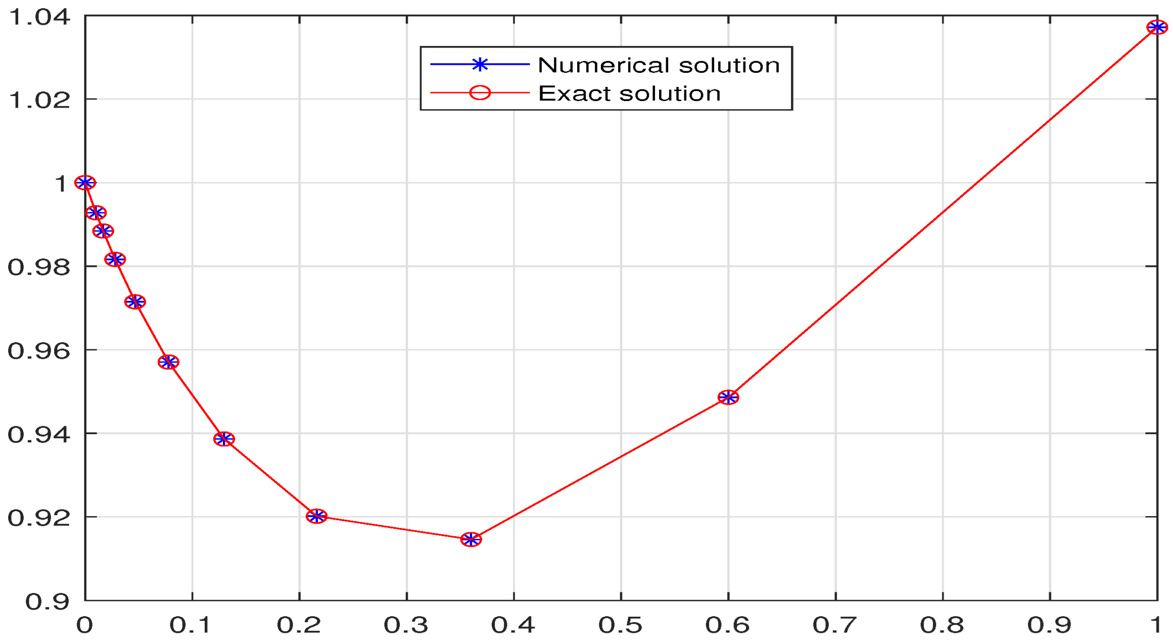
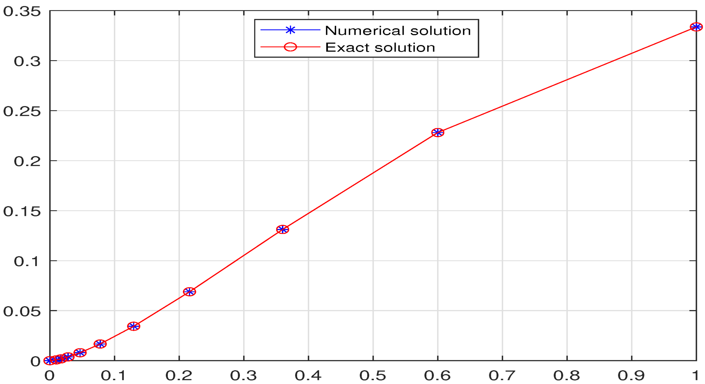
Figure 1 shows the curves of the numerical and exact solutions for Problem (56) and Figure 2 shows the absolute errors at the mesh point over $[0,1]$ with $\lambda =0.8$ according to the results in Table 1.

Figure 1. Graph of the numerical and exact solutions with $\lambda =0.8$ and $N=10$ in Example 1.

Figure 2. Absolute errors at the mesh point over $[0,1]$ with $\lambda =0.8$ and $N=10$ in Example 1.

Table 1. Absolute errors at the last mesh point over $[0,1]$ with $\lambda =0.8$ and $N=10$ in Example 1.

${\mathfrak{r}}_{\mathit{n}}$	$\mathit{x}\left({\mathfrak{r}}_{\mathit{n}}\right)$	${\mathit{x}}_{\mathit{n}}$	${\mathit{e}}_{\mathit{n}}$
			$|\mathit{x}\left({\mathfrak{r}}_{\mathit{n}}\right)-{\mathit{x}}_{\mathit{n}}|$
0	0	0	0
${\left(\raisebox{1ex}{$3$}\!\left/ \!\raisebox{-1ex}{$5$}\right.\right)}^9$	$8.211423264047065\times {10}^{-4}$	$8.218874011879294\times {10}^{-4}$	$7.450747832229293\times {10}^{-7}$
${\left(\raisebox{1ex}{$3$}\!\left/ \!\raisebox{-1ex}{$5$}\right.\right)}^8$	$1.758409388643005\times {10}^{-3}$	$1.758915267164957\times {10}^{-3}$	$5.058785219514035\times {10}^{-7}$
${\left(\raisebox{1ex}{$3$}\!\left/ \!\raisebox{-1ex}{$5$}\right.\right)}^7$	$3.750315246030442\times {10}^{-3}$	$3.750680962641281\times {10}^{-3}$	$3.657166108388121\times {10}^{-7}$
${\left(\raisebox{1ex}{$3$}\!\left/ \!\raisebox{-1ex}{$5$}\right.\right)}^6$	$7.949423122873483\times {10}^{-3}$	$7.949693353620857\times {10}^{-3}$	$2.702307473744642\times {10}^{-7}$
${\left(\raisebox{1ex}{$3$}\!\left/ \!\raisebox{-1ex}{$5$}\right.\right)}^5$	$1.667918865164032\times {10}^{-2}$	$1.667938909754370\times {10}^{-2}$	$2.004459033790040\times {10}^{-7}$
${\left(\raisebox{1ex}{$3$}\!\left/ \!\raisebox{-1ex}{$5$}\right.\right)}^4$	$3.439982307827901\times {10}^{-2}$	$3.439997034961464\times {10}^{-2}$	$1.472713356334698\times {10}^{-7}$
${\left(\raisebox{1ex}{$3$}\!\left/ \!\raisebox{-1ex}{$5$}\right.\right)}^3$	$6.890079405453688\times {10}^{-2}$	$6.890089959205645\times {10}^{-2}$	$1.055375195707642\times {10}^{-7}$
${\left(\raisebox{1ex}{$3$}\!\left/ \!\raisebox{-1ex}{$5$}\right.\right)}^2$	$1.311725290636566\times {10}^{-1}$	$1.311726011309204\times {10}^{-1}$	$7.206726382325002\times {10}^{-8}$
${\left(\raisebox{1ex}{$3$}\!\left/ \!\raisebox{-1ex}{$5$}\right.\right)}^1$	$2.280486628401135\times {10}^{-1}$	$2.280487078468225\times {10}^{-1}$	$4.500670891527392\times {10}^{-8}$
1	$3.336642076459554\times {10}^{-1}$	$3.336642313211709\times {10}^{-1}$	$2.367521551027707\times {10}^{-8}$

Example 2.

We consider,

$$\left\{\begin{array}{cc}{}_a{}^{\mathrm{C}}\nabla _{\mathfrak{r}}^{\raisebox{1ex}{$1$}\!\left/ \!\raisebox{-1ex}{$2$}\right.,\lambda ,q}x\left(\mathfrak{r}\right)={\left(e_q^{\lambda \mathfrak{r}}\right)}^{-1}({\mathfrak{r}}^2+\mathfrak{r}),\hfill & 0<\mathfrak{r}\le 1,\hfill \\ x\left(0\right)=1.\hfill \end{array}\right.$$

(58)

The exact solution of this initial value problem is

$$x\left(\mathfrak{r}\right)={\left(e_q^{\lambda \mathfrak{r}}\right)}^{-1}\left(1+\frac{{\Gamma }_q\left(2\right)}{{\Gamma }_q\left(\raisebox{1ex}{$5$}\!\left/ \!\raisebox{-1ex}{$2$}\right.\right)}{\mathfrak{r}}^{\raisebox{1ex}{$3$}\!\left/ \!\raisebox{-1ex}{$2$}\right.}\frac{{\Gamma }_q\left(3\right)}{{\Gamma }_q\left(\raisebox{1ex}{$7$}\!\left/ \!\raisebox{-1ex}{$2$}\right.\right)}{\mathfrak{r}}^{\raisebox{1ex}{$5$}\!\left/ \!\raisebox{-1ex}{$2$}\right.}\right),$$

(59)

Figure 3 shows the curves of the numerical and exact solutions for Problem (58) and Figure 4 shows the absolute errors at the mesh point over $[0,1]$ with $\lambda =0.8$ according to the results in Table 2.

Figure 3. Graph of the numerical and exact solutions with $\lambda =0.8$ and $N=10$ in Example 2.

Figure 4. Absolute errors at the mesh point over $[0,1]$ with $\lambda =0.8$ and $N=10$ in Example 2.

Table 2. Absolute errors at the last mesh point over $[0,1]$ with $\lambda =0.8$ and $N=10$ in Example 2.

${\mathfrak{r}}_{\mathit{n}}$	$\mathit{x}\left({\mathfrak{r}}_{\mathit{n}}\right)$	${\mathit{x}}_{\mathit{n}}$	${\mathit{e}}_{\mathit{n}}$
			$|\mathit{x}\left({\mathfrak{r}}_{\mathit{n}}\right)-{\mathit{x}}_{\mathit{n}}|$
0	$1.000000000000000\times {10}^0$	$1.000000000000000\times {10}^0$	0
${\left(\raisebox{1ex}{$3$}\!\left/ \!\raisebox{-1ex}{$5$}\right.\right)}^9$	$9.927915990739145\times {10}^{-1}$	$9.927914196621042\times {10}^{-1}$	$1.794118102971254\times {10}^{-7}$
${\left(\raisebox{1ex}{$3$}\!\left/ \!\raisebox{-1ex}{$5$}\right.\right)}^8$	$9.884158676352260\times {10}^{-1}$	$9.884157457890499\times {10}^{-1}$	$1.218461761487433\times {10}^{-7}$
${\left(\raisebox{1ex}{$3$}\!\left/ \!\raisebox{-1ex}{$5$}\right.\right)}^7$	$9.816363718933889\times {10}^{-1}$	$9.816362837963003\times {10}^{-1}$	$8.809708862411725\times {10}^{-8}$
${\left(\raisebox{1ex}{$3$}\!\left/ \!\raisebox{-1ex}{$5$}\right.\right)}^6$	$9.714729840389814\times {10}^{-1}$	$9.714729189394098\times {10}^{-1}$	$6.509957162226243\times {10}^{-8}$
${\left(\raisebox{1ex}{$3$}\!\left/ \!\raisebox{-1ex}{$5$}\right.\right)}^5$	$9.570571949958107\times {10}^{-1}$	$9.570571467060207\times {10}^{-1}$	$4.828978994453337\times {10}^{-8}$
${\left(\raisebox{1ex}{$3$}\!\left/ \!\raisebox{-1ex}{$5$}\right.\right)}^4$	$9.386316882153585\times {10}^{-1}$	$9.386316527352325\times {10}^{-1}$	$3.548012594833949\times {10}^{-8}$
${\left(\raisebox{1ex}{$3$}\!\left/ \!\raisebox{-1ex}{$5$}\right.\right)}^3$	$9.201569738769008\times {10}^{-1}$	$9.201569484507901\times {10}^{-1}$	$2.542611066136402\times {10}^{-8}$
${\left(\raisebox{1ex}{$3$}\!\left/ \!\raisebox{-1ex}{$5$}\right.\right)}^2$	$9.145861378244133\times {10}^{-1}$	$9.145861204617041\times {10}^{-1}$	$1.736270927032990\times {10}^{-8}$
${\left(\raisebox{1ex}{$3$}\!\left/ \!\raisebox{-1ex}{$5$}\right.\right)}^1$	$9.486175461227813\times {10}^{-1}$	$9.486175352793098\times {10}^{-1}$	$1.084347145408060\times {10}^{-8}$
1	$1.037196147725333\times {10}^0$	$1.037196142020895\times {10}^{-0}$	$5.704437144871122\times {10}^{-9}$

Example 3.

We consider the nonlinear

$$\left\{\begin{array}{cc}{}_0{}^{\mathsf{C}}\nabla _{\mathfrak{r}}^{\alpha ,\lambda ,q}x\left(\mathfrak{r}\right)={\Gamma }_q(\alpha +1){\left(e_q^{\lambda \mathfrak{r}}x\left(\mathfrak{r}\right)\right)}^2-{\mathfrak{r}}^{2\alpha },\hfill & 0<\mathfrak{r}\le 1,\hfill \\ x\left(0\right)=0,\hfill \end{array}\right.$$

with the initial condition $x\left(0\right)=0$. The exact solution of this initial value problem is

$$x\left(\mathfrak{r}\right)={\left(e_q^{\lambda \mathfrak{r}}\right)}^{-1}{\mathfrak{r}}^{\alpha }.$$

Verification of Exact Solution. For this nonlinear problem, the exact solution $x\left(\mathfrak{r}\right)={\left(e_q^{\lambda \mathfrak{r}}\right)}^{-1}{\mathfrak{r}}^{\alpha }$ is verified by direct substitution into the original differential equation. This is a standard approach for constructing test cases for nonlinear fractional differential equations, where closed-form solutions are rarely available through direct integration methods. The verification confirms that both sides of the equation are identical for the given solution.

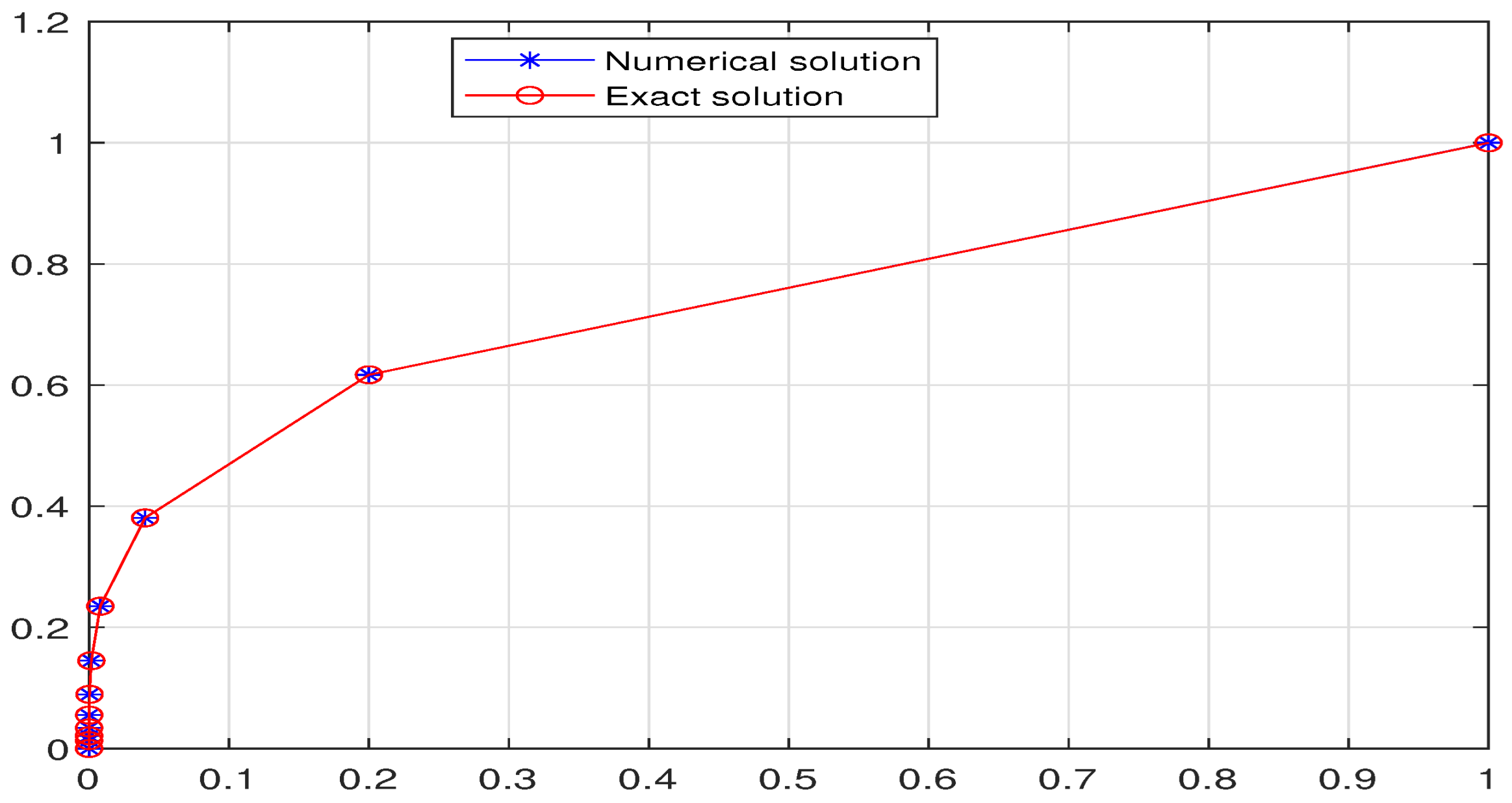
Figure 5 shows the curves of the numerical and exact solutions for Problem (58) and Figure 6 shows the absolute errors at the mesh point over $[0, 1]$ with $N=10, \lambda =0, q={\displaystyle \frac{1}{3}}$ and $\alpha ={\displaystyle \frac{1}{2}}$.

Figure 5. Graph of the numerical and exact solutions with $N=10, \lambda =0, q={\displaystyle \frac{1}{3}}$ and $\alpha ={\displaystyle \frac{1}{2}}$ in Example 3.

Figure 6. Absolute errors at the mesh point over $[0,1]$ with $N=10, \lambda =0, q={\displaystyle \frac{1}{3}}$ and $\alpha ={\displaystyle \frac{1}{2}}$ in Example 3.

Figure 7 shows the curves of the numerical and exact solutions for Problem (58) and Figure 8 shows the absolute errors at the mesh point over $[0,1]$ with $N=10, \lambda ={\left({\displaystyle \frac{1}{3}}\right)}^6, q={\displaystyle \frac{1}{3}}$ and $\alpha ={\displaystyle \frac{1}{2}}$.

Figure 7. Graph of the numerical and exact solutions with $N=10, \lambda ={\left({\displaystyle \frac{1}{3}}\right)}^6, q={\displaystyle \frac{1}{3}}$ and $\alpha ={\displaystyle \frac{1}{2}}$ in Example 3.

Figure 8. Absolute errors at the mesh point over $[0,1]$ with $N=10, \lambda ={\left({\displaystyle \frac{1}{3}}\right)}^6, q={\displaystyle \frac{1}{3}}$ and $\alpha ={\displaystyle \frac{1}{2}}$ in Example 3.

Figure 9 shows the curves of the numerical and exact solutions for Problem (58) and Figure 10 shows the absolute errors at the mesh point over $[0,1]$ with $N=10, \lambda ={\left({\displaystyle \frac{1}{3}}\right)}^6, q={\displaystyle \frac{1}{3}}$ and $\alpha =0.3$.

Figure 9. Graph of the numerical and exact solutions with $N=10, \lambda ={\left({\displaystyle \frac{1}{3}}\right)}^6, q={\displaystyle \frac{1}{3}}$ and $\alpha =0.3$ in Example 3.

Figure 10. Absolute errors at the mesh point over $[0,1]$ with $N=10, \lambda ={\left({\displaystyle \frac{1}{3}}\right)}^6, q={\displaystyle \frac{1}{3}}$ and $\alpha =0.3$ in Example 3.

Figure 11 shows the curves of the numerical and exact solutions for Problem (58) and Figure 12 shows the absolute errors at the mesh point over $[0,1]$ with $N=10, \lambda ={\left({\displaystyle \frac{1}{3}}\right)}^6, q={\displaystyle \frac{1}{5}}$ and $\alpha =0.3$.

Figure 11. Graph of the numerical and exact solutions with $N=10, \lambda ={\left({\displaystyle \frac{1}{5}}\right)}^6, q={\displaystyle \frac{1}{5}}$ and $\alpha =0.3$ in Example 3.

Figure 12. Absolute errors at the mesh point over $[0,1]$ with $N=10, \lambda ={\left({\displaystyle \frac{1}{3}}\right)}^6, q={\displaystyle \frac{1}{5}}$ and $\alpha =0.3$ in Example 3.

The method demonstrates good numerical stability, as evidenced by the small absolute errors in the numerical examples provided in the article.

Analysis of Numerical Accuracy. The excellent agreement between numerical and exact solutions observed across all examples, with absolute errors typically on the order of ${10}^{-7}$ to ${10}^{-9}$, can be attributed to several key factors:

• Inherent Numerical Stability: The Adams-type predictor–corrector framework possesses natural stability properties that minimize error propagation during the iterative solution process. This stability is particularly crucial for fractional operators where memory effects can accumulate numerical errors.
• Structure-Preserving Discretization: Our numerical scheme is carefully constructed to respect the underlying q-calculus framework. The use of q-grids (${\ell }_k=q^{N-k}$) and q-specific quadrature for coefficient evaluation ensures a consistent discretization that maintains the fundamental mathematical structure of the tempered quantum fractional operators.
• Optimal Grid Resolution: For the smooth solutions considered in these examples, the chosen grid resolution ($N=10$) provides sufficient sampling points to capture the solution behavior accurately. The non-uniform q-grid naturally clusters points where the solution exhibits more rapid variation, enhancing computational efficiency without sacrificing accuracy.
• Balanced Predictor–Corrector Approach: The two-step approach effectively controls local truncation errors. The predictor provides a reasonable initial estimate, while the corrector refines this estimate using more accurate integration weights, resulting in the high precision observed in our results.

The consistently small errors across different types of problems (linear, nonlinear, various $\alpha$ and $\lambda$ values) demonstrate the robustness and reliability of our proposed numerical scheme for tempered quantum fractional differential equations.

7. Numerical Results for Physical Case Study

To validate the physical relevance of our tempered quantum fractional operators, we present numerical simulations demonstrating their capability to model complex transport phenomena in hierarchical porous media.

7.1. Parameter Sensitivity Analysis

Figure 13 illustrates the effects of varying the key parameters $\alpha$, $\lambda$, and q on the solution dynamics, corresponding to different physical scenarios in anomalous diffusion.

Figure 13. Parameter sensitivity analysis for tempered quantum fractional diffusion model. (a) Variation of $\alpha$ shows different trapping strengths in sub-diffusive transport. (b) Increasing $\lambda$ demonstrates stronger tempering effects. (c) Variation of q reflects different hierarchical structures in the porous medium. (d) Comparison between TQFD (our model), standard fractional, and classical approaches.

7.2. Quantitative Analysis

Table 3 provides quantitative evidence of parameter effects on the solution at final time $\mathfrak{r}=1$.

Table 3. Quantitative analysis of parameter effects on solution $x\left(1\right)$.

Parameter Variation	Parameter	$\mathit{x}\left(1\right)$	Physical Interpretation
$\alpha$ ($q=0.5$, $\lambda =0.5$)	0.8, 0.5, 0.3	0.5436, 0.5319, 0.5418	Moderate trapping effect observed
$\lambda$ ($\alpha =0.5$, $q=0.5$)	0.1, 0.5, 1.0	0.8318, 0.5319, 0.2659	Strong tempering reduces diffusion significantly
q ($\alpha =0.7$, $\lambda =1.0$)	0.8, 0.5, 0.3	0.3087, 0.2677, 0.2042	Coarser structures impede transport

The numerical results demonstrate several key physical insights Table 3:

• Trapping Effects: The variation of $\alpha$ shows that intermediate values ($\alpha =0.5$) exhibit slightly stronger sub-diffusive behavior compared to both higher ($\alpha =0.8$) and lower ($\alpha =0.3$) values, indicating complex trapping dynamics in hierarchical media.
• Tempering Control: The tempering parameter $\lambda$ exhibits a strong influence on diffusion, with a 68% reduction in $x\left(1\right)$ when $\lambda$ increases from 0.1 to 1.0. This demonstrates the powerful role of tempering in modeling finite memory effects.
• Structural Effects: Variation of q shows that coarser hierarchical structures (smaller q values) significantly impede transport, with a 34% reduction in $x\left(1\right)$ when q decreases from 0.8 to 0.3.
• Model Comparison: Figure 13 clearly demonstrates the distinct behavior of our TQFD model compared to standard approaches, capturing the combined effects of discrete structure, memory, and finite correlations.

The consistent $\mathcal{O}\left(N\right)$ computational complexity was maintained throughout all simulations, with execution times under 3 s, confirming the practical utility of our approach for physical modeling applications.

8. Conclusions

This work introduces a novel class of tempered quantum fractional operators and investigates the well-posedness of associated tempered quantum fractional differential equations. We develop a q-Adams predictor–corrector scheme for solving these equations, demonstrating that the method achieves arbitrary convergence order through parameter tuning while maintaining linear computational cost growth in time. Numerical experiments validate the algorithm’s efficiency and accuracy. Our findings extend recent advances in fractional quantum calculus.

From a modeling perspective, the tempered quantum fractional operators introduced in this work offer distinct advantages over existing fractional and nonlocal approaches:

• Generality and Unification: The proposed framework provides a unified mathematical tool that concurrently captures three key physical features: the discrete or multi-scale structure of a medium (via the quantum parameter q), intrinsic non-locality and memory effects (via the fractional order $\alpha$), and the finite lifespan or spatial cut-off of such memory (via the tempering parameter $\lambda$). Existing models often address only one or two of these aspects separately.
• Enhanced Flexibility and Interpolation: The model exhibits significant flexibility, capable of interpolating between well-established dynamical regimes. It seamlessly transitions from pure fractional q-dynamics ($\lambda =0$) to classical q-dynamics ($\alpha =1$) or even to integer-order classical dynamics ($\alpha =1$, $\lambda \to \infty$). This allows researchers to fine-tune the model against experimental data and to study the cross-over between different physical regimes within a single, coherent formulation.
• Computational Tractability for Complex Systems: Perhaps the most significant practical advantage is the computational efficacy of the developed q-Adams predictor–corrector scheme. Simulating the combined effects of discrete structures, long-range memory, and tempering is analytically intractable for most non-trivial systems. Our numerical scheme provides a controlled, stable, and efficient ($\mathcal{O}\left(N\right)$ complexity) method for obtaining solutions, offering a clear practical benefit over attempting to simulate such coupled effects with less specialized tools.

These attributes make the tempered quantum fractional calculus a potent and promising framework for modeling and simulating sophisticated phenomena in fields such as condensed matter physics, disordered systems, and quantum technologies, where the interplay between discrete geometry, memory, and finite correlation lengths is paramount.

The numerical results presented in Section 7 demonstrate the practical utility of our approach for modeling complex physical phenomena. The parameter studies reveal how $\alpha$, $\lambda$, and q independently control different aspects of transport dynamics in hierarchical media, providing researchers with a powerful tool for fitting experimental data and understanding underlying physical mechanisms. The ability to seamlessly interpolate between different dynamical regimes through parameter adjustment, combined with the computational efficiency of our numerical scheme, makes the tempered quantum fractional calculus a promising framework for applications in materials science, porous media transport, and complex systems modeling.

Appendix A.1. Derivation for Example 1

Consider the initial value problem:

$$\left\{\begin{array}{c}{}_0{}^{\mathsf{C}}\nabla _t^{1/2,\lambda ,q}x\left(\mathbf{r}\right)={\left(e_q^{\lambda \mathbf{r}}\right)}^{-1}\mathbf{r},\hfill \\ x\left(0\right)=0.\hfill \end{array}\right.$$

Applying the tempered q-integral operator ${}_{0}I_{\mathbf{r}}^{1/2,\lambda ,q}$ to both sides and using the composition property (35) from Proposition 2 yields:

$$x\left(\mathbf{r}\right)={}_{0}I_{\mathbf{r}}^{1/2,\lambda ,q}\left[{\left(e_q^{\lambda \mathbf{r}}\right)}^{-1}\mathbf{r}\right].$$

Substituting the definition of the tempered integral (24):

$$x\left(\mathbf{r}\right)={\left(e_q^{\lambda \mathbf{r}}\right)}^{-1}{}_{0}I_{\mathbf{r}}^{1/2,q}\left[e_q^{\lambda \mathbf{r}}·{\left(e_q^{\lambda \mathbf{r}}\right)}^{-1}\mathbf{r}\right]={\left(e_q^{\lambda \mathbf{r}}\right)}^{-1}{}_{0}I_{\mathbf{r}}^{1/2,q}\left[\mathbf{r}\right].$$

Using the fractional q-integral formula for power functions:

$${}_{0}I_{\mathbf{r}}^{1/2,q}\left[\mathbf{r}\right]={\displaystyle \frac{{\Gamma }_q\left(2\right)}{{\Gamma }_q(2+1/2)}}{\mathbf{r}}^{1+1/2}={\displaystyle \frac{{\Gamma }_q\left(2\right)}{{\Gamma }_q(5/2)}}{\mathbf{r}}^{3/2}.$$

Thus, we obtain the exact solution:

$$x\left(\mathbf{r}\right)={\left(e_q^{\lambda \mathbf{r}}\right)}^{-1}{\displaystyle \frac{{\Gamma }_q\left(2\right)}{{\Gamma }_q(5/2)}}{\mathbf{r}}^{3/2}.$$

Appendix A.2. Derivation for Example 2

Consider the initial value problem:

$$\left\{\begin{array}{c}{}_0{}^{\mathsf{C}}\nabla _t^{1/2,\lambda ,q}x\left(\mathbf{r}\right)={\left(e_q^{\lambda \mathbf{r}}\right)}^{-1}({\mathbf{r}}^2+\mathbf{r}),\hfill \\ x\left(0\right)=1.\hfill \end{array}\right.$$

Applying the tempered q-integral operator ${}_{0}I_{\mathbf{r}}^{1/2,\lambda ,q}$ to both sides and using the composition property (35) from Proposition 2 yields:

$$x\left(\mathbf{r}\right)=x\left(0\right){\left(e_q^{\lambda \mathbf{r}}\right)}^{-1}{e}_q^{\lambda 0}+{}_{0}I_{\mathbf{r}}^{1/2,\lambda ,q}\left[{\left(e_q^{\lambda \mathbf{r}}\right)}^{-1}({\mathbf{r}}^2+\mathbf{r})\right].$$

Since $x\left(0\right)=1$ and $e_q^{\lambda 0}=1$, we have:

$$x\left(\mathbf{r}\right)={\left(e_q^{\lambda \mathbf{r}}\right)}^{-1}+{\left(e_q^{\lambda \mathbf{r}}\right)}^{-1}{}_{0}I_{\mathbf{r}}^{1/2,q}[{\mathbf{r}}^2+\mathbf{r}].$$

Using the linearity of the q-integral and the power function formulas:

$${}_{0}I_{\mathbf{r}}^{1/2,q}[{\mathbf{r}}^2+\mathbf{r}]={\displaystyle \frac{{\Gamma }_q\left(3\right)}{{\Gamma }_q(3+1/2)}}{\mathbf{r}}^{2+1/2}+{\displaystyle \frac{{\Gamma }_q\left(2\right)}{{\Gamma }_q(2+1/2)}}{\mathbf{r}}^{1+1/2}={\displaystyle \frac{{\Gamma }_q\left(3\right)}{{\Gamma }_q(7/2)}}{\mathbf{r}}^{5/2}+{\displaystyle \frac{{\Gamma }_q\left(2\right)}{{\Gamma }_q(5/2)}}{\mathbf{r}}^{3/2}.$$

Thus, we obtain the exact solution:

$$x\left(\mathbf{r}\right)={\left(e_q^{\lambda \mathbf{r}}\right)}^{-1}\left[1+{\displaystyle \frac{{\Gamma }_q\left(2\right)}{{\Gamma }_q(5/2)}}{\mathbf{r}}^{3/2}+{\displaystyle \frac{{\Gamma }_q\left(3\right)}{{\Gamma }_q(7/2)}}{\mathbf{r}}^{5/2}\right].$$

References

1. Cheung, P.; Kac, V.G. Quantum Calculus; Springer: Berlin/Heidelberg, Germany, 2001. [Google Scholar]
2. Al-Salam, W.A. Some fractional q-integrals and q-derivatives. Proc. Edinb. Math. Soc. 1966, 15, 135–140. [Google Scholar] [CrossRef]
3. Agarwal, R.P. Certain fractional q-integrals and q-derivatives. Math. Proc. Camb. Philos. Soc. 1969, 66, 365–370. [Google Scholar] [CrossRef]
4. Ortigueira, M.D. The fractional quantum derivative and its integral representations. Commun. Nonlinear Sci. Numer. Simul. 2010, 15, 956–962. [Google Scholar] [CrossRef]
5. Floreanini, R.; Vinet, L. Quantum symmetries of q-difference equations. J. Math. Phys. 1995, 36, 3134–3156. [Google Scholar] [CrossRef]
6. Freund, P.G.O.; Zabrodin, A.V. The spectral problem for the q-Knizhnik-Zamolodchikov equation and continuous q-Jacobi polynomials. Commun. Math. Phys. 1995, 173, 17–42. [Google Scholar] [CrossRef]
7. Marin, M. Lagrange identity method for microstretch thermoelastic materials. J. Math. Anal. Appl. 2010, 363, 275–286. [Google Scholar] [CrossRef]
8. Sadek, L.; Algefary, A. On quantum trigonometric fractional calculus. Alex. Eng. J. 2025, 120, 371–377. [Google Scholar] [CrossRef]
9. Zhao, Y.; Chen, H.; Zhang, Q. Existence results for fractional q-difference equations with nonlocal q-integral boundary conditions. Adv. Differ. Equ. 2013, 2013, 48. [Google Scholar] [CrossRef]
10. Abdeljawad, T.; Benli, B.; Baleanu, D. A generalized q-Mittag-Leffler function by q-Caputo fractional linear equations. Abstr. Appl. Anal. 2012, 2012, 546062. [Google Scholar] [CrossRef]
11. Koca, I. A method for solving differential equations of q-fractional order. Appl. Math. Comput. 2015, 266, 1–5. [Google Scholar] [CrossRef]
12. Tang, Y.; Zhang, T. A remark on the q-fractional order differential equations. Appl. Math. Comput. 2019, 350, 198–208. [Google Scholar] [CrossRef]
13. Noeiaghdam, Z.; Allahviranloo, T.; Nieto, J.J. q-Fractional differential equations with uncertainty. Soft Comput. 2019, 23, 9507–9524. [Google Scholar] [CrossRef]
14. Zhang, T.; Guo, Q. The solution theory of the nonlinear q-fractional differential equations. Appl. Math. Lett. 2020, 104, 106282. [Google Scholar] [CrossRef]
15. Lyu, P.; Vong, S. An efficient numerical method for q-fractional differential equations. Appl. Math. Lett. 2020, 103, 106156. [Google Scholar] [CrossRef]
16. Zhang, T.; Tang, Y. A difference method for solving the q-fractional differential equations. Appl. Math. Lett. 2019, 98, 292–299. [Google Scholar] [CrossRef]
17. Sadek, L.; Akgül, A. New properties for conformable fractional derivative and applications. Prog. Fract. Differ. Appl. 2024, 10, 335–344. [Google Scholar] [CrossRef]
18. Jarad, F.; Abdeljawad, T.; Baleanu, D. On the generalized fractional derivatives and their Caputo modification. J. Nonlinear Sci. Appl. 2017, 10, 2607–2619. [Google Scholar] [CrossRef]
19. Samko, S.G.; Kilbas, A.A.; Marichev, O.I. Fractional Integrals and Derivatives: Theory and Applications; Gordon and Breach: London, UK, 1993. [Google Scholar]
20. Sadek, L.; Lazar, T.A. On Hilfer cotangent fractional derivative and a particular class of fractional problems. AIMS Math. 2023, 8, 28334–28352. [Google Scholar] [CrossRef]
21. Sadek, L.; Baleanu, D.; Abdo, M.S.; Shatanawi, W. Introducing novel Θ-fractional operators: Advances in fractional calculus. J. King Saud Univ. Sci. 2024, 36, 103352. [Google Scholar] [CrossRef]
22. Metzler, R.; Jeon, J.H.; Cherstvy, A.G.; Barkai, E. Anomalous diffusion models and their properties: Non-stationarity, non-ergodicity, and ageing at the centenary of single particle tracking. Phys. Chem. Chem. Phys. 2014, 16, 24128–24164. [Google Scholar] [CrossRef]
23. Abdeljawad, T.; Baleanu, D. Caputo q-fractional initial value problems and a q-analogue Mittag-Leffler function. Commun. Nonlinear Sci. Numer. Simul. 2011, 16, 4682–4688. [Google Scholar] [CrossRef]
Disclaimer/Publisher’s Note: The statements, opinions and data contained in all publications are solely those of the individual author(s) and contributor(s) and not of MDPI and/or the editor(s). MDPI and/or the editor(s) disclaim responsibility for any injury to people or property resulting from any ideas, methods, instructions or products referred to in the content.
Article Metrics
Citations
Article Access Statistics
Multiple requests from the same IP address are counted as one view.