Abstract
We are concerned in this paper with the stability and bifurcation problems for three-neuron-based bi-directional associative memory neural networks that are involved with time delays in transmission terms and possess Caputo fractional derivatives of non-commensurate orders. For the fractional bi-directional associative memory neural networks that are dealt with in this paper, we view the time delays as the bifurcation parameters. Via a standard contraction mapping argument, we establish the existence and uniqueness of the state trajectories of the investigated fractional bi-directional associative memory neural networks. By utilizing the idea and technique of linearization, we analyze the influence of time delays on the dynamical behavior of the investigated neural networks, as well as establish and prove several stability/bifurcation criteria for the neural networks dealt with in this paper. According to each of our established criteria, the equilibrium states of the investigated fractional bi-directional associative memory neural networks are asymptotically stable when some of the time delays are less than strictly specific positive constants, i.e., when the thresholds or the bifurcation points undergo Hopf bifurcation in the concerned networks at the aforementioned threshold constants. In the meantime, we provide several illustrative examples to numerically and visually validate our stability and bifurcation results. Our stability and bifurcation theoretical results in this paper yield some insights into the cause mechanism of the bifurcation phenomena for some other complex phenomena, and this is extremely helpful for the design of feedback control to attenuate or even to remove such complex phenomena in the dynamics of fractional bi-directional associative memory neural networks with time delays.
1. Introduction
In the last several decades, neural networks (NNs) have been found to be of wide applicability in areas such as in the recognition and/or classification of patterns, signal processing, engineering optimization and associative memory (see [1,2,3,4,5] and the references cited therein). To improve some of their specific application capabilities, experts have created various types of NNs with special structural features in recent years (see references [1,3,5,6]). For example, Kosko (1980s) [2,3] constructed a class of NNs that are contemporarily known as bidirectional associative memory neural networks (BAMNNs). Kosko created this class with the desire to extend a single-layer auto-associative Hebbian correlator to two-layer pattern-matched hetero-associative circuits (see references [6,7]). In the last three decades or so, for the purpose of understanding how the application performance could be improved, BAMNNs have been both extensively and intensively studied in the literature.
Among the vast number of studies that have reported research results concerning BAMNNs, there are two categories of results that have their own tremendous attractiveness: those regarding stability and synchronizability. As the new researching methods and techniques become more and more advanced, a large number of experts have reported interesting results concerning the stability of BAMNNs (see references [3,6,7,8,9,10]). For example, Kosko [3] made several remarks on the stability and related properties of BAMNNs. Inspired by the results in reference [3] and in some other related results, Park et al. [7] established a new stability criterion for neutral-type BAMNNs. Based on the previous results obtained in studies such as [3,6,7], Zhu Li et al. [8] reported an interesting exponential stability result for stochastic reaction–diffusion BAMNNs with time-varying and distributed delays. As is the case with research on the stability problem, a huge number of results concerning the synchronization problem for BAMNNs have also been reported publicly in recent years (see [11,12,13]). Stability and synchronizability are closely related notions, and they both guarantee that NNs display outstanding application performance (see, for instance, references [3,10,14,15,16]).
In quite a few situations, the aftereffect (or memory) of BAMNNs (or NNs, more generally) cannot be neglected. One feasible way through which to portray the aftereffect is to incorporate a time delay in the BAMNNs. Another sensible way through which to describe the aftereffect is to replace the derivatives of the integer orders with those of non-integer (or fractional, more generally) orders in BAMNNs (see, for example, references [17,18]). In this paper, we are mainly concerned with those BAMNNs whose aftereffect can be described by time delays and/or fractional-order derivatives in the Caputo sense, which we shall explain in greater detail in Section 2 (especially its Definition 1). As usual, we shall call BAMNNs (i.e., NNs) with a time delay DBAMNNs (i.e., DNNs), and—similarly—we shall call BAMNNs (i.e., NNs) with derivatives of fractional orders FBAMNNs (i.e., FNNs). In some special cases, the time delays and/or derivatives of non-integer orders do contribute to the stability and/or synchronizability of BAMNNs (or to NNs, more generally). But, generally speaking, time delays and/or derivatives of non-integer orders can cause tremendous troubles for us in trying to prove the stability and/or synchronizability of BAMNNs (or NNs, more generally). In order to attenuate or even remove such troubles, experts have developed several methods and have reported a great deal of interesting and inspirational results based on these methods. The interested readers can consult the studies of [6,8,10,11,13,14,16,19,20,21] for more detailed explanations of the more meaningful results in this respect. Let us point out that, in these references, the method of Lyapunov–Krasovskii functionals has been widely utilized and quite impressive advances have been established via this approach. But it seems that the structural property, the time delay, and/or the derivatives of non-integer orders, say, of BAMNNs (or NNs, more generally) have not been explored thoroughly. In recent years, an increasing amount of attention has been paid to the study of the structural property of BAMNNs (or NNs, more generally) as there is a strong desire to better understand the stability and synchronizability of BAMNNs (or NNs, more generally). In this respect, interested readers can consult the studies of [22,23,24,25,26,27,28,29] for more detailed explanations on the recent advances.
To make more clear our motivation for the research in this paper, we would like to introduce and remark briefly on the results in the studies of [22,23,24,25,26,27,28,29]. Deng Li et al. [22] provided a spectral criterion (see Lemma 3 in Section 2) that can guarantee the stability of the linear systems of Caputo fractional-differential equations with discrete time delays. The spectral result in reference [22] has been of great importance for later studies on the dynamics of systems of fractional differential equations with (discrete) time delays. Li Yan et al. [23] analyzed the dynamic bifurcation phenomenon, say, of fractional-order tri-neuron neural networks incorporating time delays. Xu Mu et al. [24] conducted a careful bifurcation analysis on a class of fractional-order neural networks incorporating two different time delays. Xu Liu et al. [25] investigated the mechanism of the bifurcation phenomenon in a class of fractional-order three-triangle multi-delayed neural networks. Xu Zhang et al. [26] studied the bifurcation phenomenon of fractional-order three-layer neural networks with four time delays. Xu Liao et al. [27] analyzed the influence of the leakage delay in the bifurcation of fractional-order complex-valued neural networks. Xu Aouiti et al. [28] conducted a comparative analysis on a Hopf bifurcation of integer-order and fractional-order two-neuron NNs with delays. Inspired by the results obtained in reference [28], Xu Mu et al. [29] investigated the bifurcation behavior of integer-order and fractional-order DBAMNNs. The results in some of the references (i.e., [22,23,24,25,26,27,28,29]) have prompted many more related works in recent years. Among these results, one category has been mainly oriented toward analyses of the influence of (discrete) time delays on the dynamics of BAMNNs of differential equations with integer-order or fractional-order derivatives, as well as toward designing controls to reduce or even to remove complex dynamics such as bifurcation. Among the vast amount of existing studies, the references of [30,31,32,33,34,35,36,37,38,39,40,41,42,43,44,45,46,47] are most closely related to the topic discussed in this paper.
The DBAMNNs studied in [30,31,32,33,34,35,36,37,38,39,40,41,42,43,44,45,46,47] and the references therein can be written as
Here, and hereafter, denotes the interval ; M and N are the two given positive integers, respectively; denotes the (first-order) time derivative of ; is the coefficient of a leakage term (or a forgetting term); is the coefficient of a transmission term; is an activation function; and , which is required to be non-negative, is the time delay, where the index parameters k and ℓ (which, in actuality, depend on k)are given such that
In view of the fruitful interesting research results concerning DBAMNN (1), attention has also been directed, in recent years, to the study of the fractional counterparts of DBAMNN (1). More precisely, the attention has been directed to FBAMNNs of the following form:
in which , which is the order of the derivative, is a non-negative real number; is a Caputo fractional-order differential operator (see Definition 1 in Section 2 for a more detailed definition); the constants , , and , as well as the function , have a similar meaning as those in DBAMNN (1); and the index parameters k and ℓ, as with those in DBAMNN (1), are given such that ℓ depends, in actuality, on k in such a way that Relation (2) is fulfilled.
Ou Xu et al. [30] studied the bifurcation control problem for BAMNN (1), including with a single time delay and with and . They analyzed the cause mechanism of the bifurcation, whose existence can be proved rigorously, as well as designed a class of feedback control to improve the dynamical behavior. As can be seen just now, in the context of DBAMNN (1) and FBAMNN (3), the DBAMNNs dealt with in Reference [30] had three neurons and therefore had a relatively simple structure. DBAMNNs that comprise more than three neurons have more complicated structural properties, and they seem to be more difficult to study in terms of their dynamics. Therefore, they have attracted more extensive attention from researchers.
DBAMNNs with four neurons have been studied by several researchers (see, for instance, References [31,32,33],). Xu Zhang et al. [31] analyzed the dynamical properties of FBAMNN (3) with and , as well as with a commensurate-order Caputo fractional derivative. Yu and Cao [32] investigated DBAMNN (1) with , as well as with two distinct time delays for its stability and the Hopf bifurcation phenomenon. Inspired by previous interesting results, Xu Zhang et al. [33] studied a fractional counterpart of the DBAMNN dealt with in Reference [32] (that is, FBAMNN (3) with and with a commensurate-order Caputo fractional derivative) regarding further stability and Hopf bifurcation results. Furthermore, Xu Zhang et al. [33] proposed a feedback control law with the aid of these obtained bifurcation analysis results to improve the dynamical behavior of the FBAMNN they were concerned with.
DBAMNNs with five neurons have also been studied by quite a few experts (see, for example, References [34,35,36]). Yang and Ye [34] performed stability and bifurcation analysis on a simplified five-neuron BAMNN with delays. The model dealt with in Reference [34] can be rewritten as DBAMNN (1) with and , which has a relatively simple structure (in the context of DBAMNNs with five neurons) and was illuminating for later related studies. The results obtained by Yang and Ye [34] helped us to better understand the influence of time delays on the complicated dynamical behaviors (e.g., the bifurcation phenomenon) of DBAMNNs. Illuminated by the results in Reference [34], Li Lu, et al. [35] studied a fractional counterpart of the DBAMNN in Reference [34], which is an FBAMNN that can be written the same as DBAMNN (3) with , and with a commensurate-order Caputo fractional derivative. In addition, they also designed a delayed feedback control to control the bifurcation based on the results obtained from the dynamics of the FBAMNN studied in Reference [35]. Xu Aouiti et al. [36] studied the bifurcation problem for FBAMNN (3) with a commensurate-order Caputo fractional derivative.
Compared with that of DBAMNNs that comprise three/four/five neurons, the analysis of dynamics of DBAMNNs with six neurons have been studied by quite a large number of researchers (see, for instance, References [37,38,39,40,41,42,43,44,45]). Liu Li et al. [37] conducted high codimensional bifurcation analyses of DBAMNN (1) with and . Li Liao et al. [38] performed elaborate analyses on the dynamical behavior of FBAMNN (3) with a commensurate-order Caputo fractional derivative. Huang Li et al. [39] conducted a dynamical analysis on DBAMNN (1) with and . Xu Liu et al. [40] explored the bifurcation phenomenon of FBAMNN (3) with and , as well as with a commensurate-order Caputo fractional derivative. In order to extend the results in References [39,40], Li Liao et al. [41] analyzed the dynamics of FBAMNN (3) with and , as well as with Caputo fractional derivatives of non-commensurate orders. Wang, Xu et al. [42] conducted some further explorations on the bifurcation provoked by a single time delay for FBAMNN (3) with . Li Lu et al. [43] investigated a class of time-delayed FBAMNNs with six neurons, in which they displayed a symmetric structure, as well as designed a bifurcation control law to improve the dynamical behavior. Xu Mu et al. [44] probed into the influence of several distinct discrete time delays on the bifurcation property of FBAMNN (3) with , as well as with a commensurate-order Caputo fractional derivative. Li Liao et al. [45] studied the bifurcation problem for FBAMNN (3) with , as well as with Caputo fractional derivatives of non-commensurate orders.
Some researchers have been attracted to studying DBAMNNs with more than six neurons (see, for example, References [46,47]). Xu Liu et al. [46] considered FBAMNN (3) with and with two distinct time delays, and they obtained some interesting results concerning the stability and bifurcation phenomenon of their studied FBAMNN. In comparison with BAMNNs, which have been frequently investigated (such as in References [30,31,32,33,34,35,36,37,38,39,40,41,42,43,44,45]), the FBAMNN dealt with in Reference [46] seemingly demonstrated a more complicated structure. Therefore, the results in Reference [46] were found to be relatively thought-provoking for later related studies of BAMNNs. Wang Cao et al. [47] studied the bifurcation problem and some other related problems for a class of FBAMNNs with neurons and mixed time delays, that is, for the following FBAMNN:
in which, n is a generic positive integer and is a non-negative constant, which represents the time delay in the leakage (forgetting) terms that were proved under certain conditions in terms of the time delay , the time delays , (), as well as and () in transmission terms. These were related to the studied FBAMNN that could display Hopf bifurcation. The FBAMNNs dealt with in Reference [47] were of a quite general form. Therefore, the profound results in Reference [47] were found to be illuminating for later related studies. As opposed to References [30,31,32,33,34,35,36,37,38,39,40,41,42,43,44,45,46], and, as with Reference [27], Wang Cao et al. [47] took into account a (single) time delay in leakage (or forgetting) terms, and this was studied apart from time delays in transmission terms.
By reviewing the studies of [30,31,32,33,34,35,36,37,38,39,40,41,42,43,44,45,46,47] and the other vast number of cited references therein, we can conclude that it would essentially become more difficult to treat the stability and the bifurcation problems for DBAMNNs as the number of neurons that comprise them become greater. This could result in more new ideas and methods being created in the procedure of treating problems associated with DBAMNNs with a relatively large number of neurons. These new ideas and methods are certainly helpful for the treatment of DBAMNNs that have a complicated structure.
Inspired by the profound interesting results presented in the aforementioned references (see References [22,23,24,25,26,27,28,29], as well as References [30,31,32,33,34,35,36,37,38,39,40,41,42,43,44,45,46,47], for more detailed explanations), we are particularly motivated by the results obtained in References [30,41,45] in terms of studying the stability and the bifurcation problems for FBAMNN (3) with Caputo fractional derivatives of non-commensurate orders with and —that is, for a class of FBAMNNs that can be written in the following form:
where the orders , and of the Caputo fractional derivatives are not necessarily identical; the coefficients , and in the leakage (forgetting) terms are all strictly positive; the connection weights (that is, the coefficients in transmission terms) , , and are all real constants; the activation functions , , and defined in are all real valued functions having some regularity (which will specified explicitly later); and the discrete time delays , , and are all non-negative constants. Some additional restrictions, in terms of , , , , , , , , , , , , , , , , and will be formulated explicitly at the right position in due time.
Assumption 1.
and , . The transmission coefficients , , and are all real constants. The time delays , , and are all non-negative.
Assumption 2.
The activation functions and belong to the . They also belong to the totality of continuous functions, whereby is mapped into itself, and have the continuous first-order derivatives of , as well as the first-order derivatives of and at 0, which are both non-zero and have .
The remainder of this paper is organized as follows. In Section 2, we recall some preliminaries that are necessary for our later presentation. In Section 3, we state our principal results and present their proofs in detail. In Section 4, we validate, in both numeric and visual ways, our theoretical results via bringing forward three time-delayed FBAMNNs. In Section 5, we conclude our discussion in this paper by providing some remarks.
2. Preliminaries
In this section, our main aim is to collect some preliminaries, which play essential roles in the presentation of the remainder of this paper. We shall recall, in a relatively systematic way, the notions (Definitions 1 and 2) and the basic properties (Lemmas 1–5) concerning fractional-order derivatives in a Caputo sense. Meanwhile, we shall complement Assumptions 1 and 2 with a new assumption, that is, Assumption 3.
Definition 1.
([48,49]). Let , and be given such that . The α-order fractional derivative , with respect to time t, of the function , which starts from the time instant in a Caputo sense is given formally by
where is the celebrated Euler’s Gamma function.
To facilitate our later presentation of the main concerns of this paper, we would like to recall here some useful results on the system of differential equations with derivatives of fractional orders in a Caputo sense (SCFDE) and on the time-delayed SCFDE (SDCFDE).
Definition 2.
([48,49]). Let , where N is a positive integer, T is a positive time instant, . In addition, the totality of the square matrices of order N, whose entries are all real, are and . If , written in component form as , satisfies
then is said to be a solution, specifically in the interval , to the following Cauchy problem for a system of commensurate Caputo fractional differential equations:
Via Definition 2, we can formulate the solutions to SCFDE via expressions with integrals. But it is obvious to find that such a formulation of solutions (see Definition 2 for the details) cannot sufficiently provide much help for studying in-depth SCFDE. As a consequence, we are led to recalling the counterpart of Duhamel’s principle for SCFDE. To this end, we recall now the notion of Mittag–Leffler functions. Let . Thus, we write
and call a Mittag–Leffler function. It is not difficult to prove that is an entire function on the complex plain . As with the common conventions, we shall write
Now, we are in a position to recall Duhamel’s principle for SCFDE.
Lemma 1.
([49]). Let , where N is a positive integer, T is a positive time instant and . If , is a solution, specifically in , to the following Cauchy problem (for a fractional differential equation in a Caputo sense),
then it holds that
where and are given in a way that is analogous to that of (6), which more precisely, is
where is an initial datum and is given in the Banach space . Furthermore, the totality of the continuous mapping of is placed into .
By applying Duhamel’s principle for SCFDE (i.e., Lemma 1), one can prove a Gronwall-type inequality for differential inequality with a derivative of a non-integer order.
Lemma 2.
([20]). Let , , , be given. If the function is regular enough and satisfies the following Caputo fractional differential inequality,
then it holds that
We would like to recall some techniques for a spectral analysis of SDCFDE. In the literature, spectral techniques have been used to examine carefully analyze the influence of time delays and/or derivatives of fractional orders on the dynamics of SDCFDE. Let us consider the SDCFDE
where N is a given positive integer and is the unknown. The restrictions on the constants , , , as well as , will be given explicitly in due time (see, for instance, Lemma 3). We thus associate SDCFDE (10) with the characteristic function
Lemma 3.
Lemma 4.
Let , , and be given such that . Then, for every with —as well as for every Lebesgue integrable function such that if and that is continuous in the subinterval —the expression
is well defined as a continuous function. Moreover, it also holds that
Proof.
The proof of Lemma 4 could be completed via some routine calculations. For the sake of conciseness, the details are omitted here. □
Thanks to Assumptions 1 and 2, FBAMNN (4) can be linearized into
Lemma 5.
Proof.
Aside from Assumptions 1 and 2 in Section 1, in some of our main results, we shall need the following restriction on the characteristic function (see (13) in Lemma 5).
Assumption 3.
It always holds that whenever is a solution to the algebraic equation with the two-parameter function being given as in (13).
3. The Main Results and Their Proofs
In this section, we shall present our main results and their proofs.
Our first aim in this section is to investigate the existence of the state trajectories of FBAMNN (4). To this end, we supplemented FBAMNN (4) with the following initial condition:
where , , and are given as continuous functions.
Theorem 1.
Suppose that Assumptions 1 and 2 hold true. For any given continuous function , , and , FBAMNN (4) is supplemented with the initial condition (14), which admits a unique state trajectory . More precisely, there exists a unique triple , which is required to satisfy the initial condition (14) and additionally satisfy , such that
Proof.
Without a loss of generality, we assume that , , , and are such throughout this proof. The proof of the case can be carried out similarly.
Let be given. The value of T can be altered as necessary. It is well known that , , and , which are equipped with the metrics induced by their supremum norms, are respectively complete metric spaces. We thus denote
Equipped with the product metric ,
is a complete metric space.
Let the initial data , , and be given. For every triple satisfying the initial condition (14), we associate the triple , which satisfies
as well as satisfies
Let us define a mapping on the complete metric space by
Hereafter, we shall write this as for the sake of convenience.
Let the initial data , , and be fixed as above. For any triple satisfying the initial Condition (14), as well as any triple satisfying
we have
which follows from (14) and (21). Thus, have
With Lemma 4 and the Definition (17) of the metric , this—together with (22)—implies
where , which is a class kappa function and is defined explicitly by
Let us fix the value of T with
With this choice of the value of T, we have . This, together with (23), implies that , which is defined by (20) together with (18) and (19), is a (strict) contraction mapping of the complete metric space (and this is defined as in (16)) into itself. With Banach’s fixed-point theorem, admits a unique fixed point, which will be designated by from now on, in . Again, with (20) alongside with (18) and (19), the fixed point of satisfies (14) and (15), or—equivalently—the fixed point will indeed be the unique state trajectory of the FBAMNN (4) satisfying the initial Condition (14) in the interval , with T being given by (25).
Based on the local existence and uniqueness results established above, we can complete, via a standard continuation argument, the proof of Theorem 1, where we claimed the global existence and uniqueness results for FBAMNN (4). The rest of the proof is straightforward, and therefore its details are chosen to be omitted here. □
Remark 1.
The Choice (25) of the value of T is not unique. In actuality, we could obtain a (strict) contraction mapping on the complete metric space when we fix Tsuch that
One of the merits of the proof of Theorem 1 is that we chose the value of T via an explicit expression.
Remark 2.
Through borrowing ideas from References [23,31,44], we can prove that the state trajectories of FBAMNN (4) are ultimately bounded when , , , and are such by virtue of Lemma 2. Let us point out that when , one can also prove that, under some additional appropriate conditions, the state trajectories of FBAMNN (4) are ultimately bounded. In actuality, we can provide a unified way through which to treat the two situations via utilizing the following Volterra equations:
and
which follow immediately from Lemma 1 (and can be viewed as a fractional version of Duhamel’s principle). In addition, the following integral identity plays a key role in the unified treatment:
where α and β are two given positive parameters.
To facilitate the formulation of one of our main results, we introduce with
as well as introduce with
Theorem 2.
Suppose that Assumptions 1–3 hold true. Assume, in addition, and , where the positive constants and are given by
and
respectively, and that and are defined as in (26) and (27), respectively. If , then the equilibrium state of FBAMNN (4) with is asymptotically stable. In addition, FBAMNN (4) with undergoes a Hopf bifurcation at , thus resulting in periodic orbits around the zero-equilibrium state in the phase space.
Proof.
In following the idea in [23,31,44], to prove Theorem 2, it is key to analyze the linearized FBAMNN (12) with . With Lemma 5, the characteristic equation of FBAMNN (12) with , which is the linearized system of FBAMNN (4) with , can be written into the following form:
(see (13) for a definition of . By Lemma 5 (particularly (13)), we have
We shall now investigate the positive solutions to the characteristic equation on the imaginary axis. Let us write
With this at our disposal, we have
Analogously, we have the following identities
and
Now, plug (32)–(37) into (30) to obtain
With the help of Equation (38), via some routine but tedious calculations, we can conclude that the identity is equivalent to
in which , , , and are given by
and
respectively. Thanks to and , Equation (39) is equivalent to
Equation (44)1 is equivalent to with , and is given by
Now, plug + (40)–(43) into (45) to arrive at
where the constant is given by (26), and , are given by
respectively. By the Definitions (47)–(51), it follows that
This, together with (46), implies immediately that (see Equation (26) for the definition of the constant ). In addition, it is not difficult to conclude that
By recalling the limit theory of functions, there exists a constant such that . Therefore, via the intermediate value theorem for continuous functions, we can conclude that there exists a constant such that . Let us begin to solve the following algebraic equation with as the unknown:
With Euler’s identity and some computations, we can find that Equation (54) is equivalent to
which directly implies
where is any given integer that renders the right hand side of Equation (56) as positive, and and are given by
and
respectively, in which , , and are defined by
and
respectively. Combine (56)–(61) to conclude that the positive constant (i.e., ) is given by Equation (28) (i.e., Equation (29)) and is well defined.
Differentiate the function of , whose implicit correspondence relation is given by (see Equation (30) for the definition of ), to arrive at
which, alongside some complicated calculations, implies
where and are given by
and
respectively. To proceed further, we conducted the computations using Equation (31):
By recalling the well-known Euler’s identity, we plugged (65) into (63) to obtain
in which and are given by
and
respectively.
As with (26) and (27), for the sake of convenience, we will introduce with
as well as introduce with
Theorem 3.
Suppose that Assumptions 1–3 hold true. Assume, in addition, and , where the positive constants and are given by
and
respectively. and are defined as in (74) and (75), respectively. If , then the equilibrium state of FBAMNN (4) with is asymptotically stable. In addition, FBAMNN (4) with undergoes a Hopf bifurcation at , thus resulting in periodic orbits around the zero equilibrium state in the phase space.
Proof.
In view of the special structure of FBAMNN (4), we can see that the proof of Theorem 3 is parallel to that of Theorem 2; hence, we choose to omit its details here. □
Theorem 4.
Suppose that Assumptions 1–3 hold true. Assume, in addition, and , where the positive constants and are given by
and
respectively, and where and are defined as in (78) and (79), respectively. If , then the equilibrium state of FBAMNN (4) with is asymptotically stable. In addition, FBAMNN (4), with , undergoes a Hopf bifurcation at , thus resulting in periodic orbits around the zero equilibrium state in the phase space.
Proof.
As with the proofs of Theorems 2 and 3, we shall prove Theorem 4 via following the idea in References [23,31,44]. More precisely, we shall analyze the characteristic equation (see Lemma 5 for the details) of the linearized FBAMNN (12) with , which is (locally) topologically equivalent to FBAMNN (4) with . In view of Equation (13) in Lemma 5, we can write, in an explicit way, the characteristic equation of FBAMNN (12) as
As in the proofs of Theorems 2 and 3, we are interested in the solutions to the characteristic equation on the imaginary axis. Therefore, we assume that is given as in Equation (31). Recalling (32)–(37), we have, via some laborious calculations, the following:
With this at our hand, we can find that the equation is equivalent to
in which, , , , and are given by
and
respectively. By taking steps that are similar to those utilized to obtain the equivalence between (44) and (39), we can easily find that Equation (84) is, in actuality, equivalent to
Evidently, Equation (89)1 is equivalent to with being given by
By taking steps that are analogous to those used to derive (46) from (40)–(43) and (45), with the aid of (85)–(88), we can deduce from (90) that
applies, where is given by (78), and , are given by
respectively.
and
where is exactly the one given by (51). By the Definitions (92)–(96), it follows that , . This, alongside (91), implies directly that (see Equation (78) for the definition of the constant ). In addition, it is not difficult to conclude that . By recalling the limit theory of functions, there exists a constant such that . Therefore, by the intermediate value theorem for continuous functions, we conclude that there exists a constant such that . Via Euler’s identity and some computations, we can find that Equation (89) is equivalent to
This immediately implies that
where is any given integer that renders the right hand side of Equation (98) as positive, and where and are given by
and
respectively. In the former , , and are given by
and
respectively. Combine (98)–(103) to conclude that the positive constant (i.e., ) given by Equation (80) (i.e., Equation (81)) is well defined.
Differentiate the function of , whose implicit correspondence relation is given by (see Equation (82) for the definition of ), to give
By steps that are analogous to those used to derive (62), we can deduce from (104) that
where and are given by
and
respectively. As in the proof of Theorem 2, we are mainly interested in the behaviors of on the imaginary axis. Therefore, we assume that is given by (31). In mimicking the steps to derive (65), we can easily prove
and
With (33), (108), and (109) as the main tools, we could deduce from (106) that
where and are given by
and
respectively. With the help of (33)–(37), (108), and (109), we can deduce from (107) that
where and are given by
and
respectively. In mimicking the steps employed to prove (72), we plugged (110) and (113) into (105) to arrive at
In recalling the definition (79) of , we mimicked the steps taken to deduce (73) and combined (110)–(114), as well as (115), to obtain
This, together with (116), implies
By recalling the assumption that , as well as by utilizing the steps analogous to those taken to prove Theorem 2, we can deduce from (117) that
This, together with the Definition (80) of , implies that the proof is complete. □
Remark 3.
As alluded to above, the idea utilized to prove Theorems 2–4, were widely used in a large number of references such as [23,31,44]. As can be seen from the proof of Theorems 2 and 4, our idea was employed to prove the claimed asymptotical stability (at least locally), which is to apply Lemma 3 and to verify that all of the roots of the characteristic equations of the linearized FBAMNNs of the concerned FBAMNNs (see FBAMNN (4) and FBAMNN (12) for the details) have negative real parts; our idea was utilized to prove the Hopf bifurcation result claimed in Theorem 2 to be also analogous to those used in [23,31,44]. In the latter idea, it is extremely vital to verify that there exists a positive constant such that the equation (where ϱ is the unknown and is given as in Equation (13) in Lemma 5) admits a positive solution, which is denoted by , thus fulfilling the property that , where μ is the implicit function of ζ that is determined by near the point . It is straightforward to find that the latter idea was also employed to prove the Hopf bifurcation results claimed in Theorems 3 and 4.
4. Illustrative Examples
Example 1.
Let , as well as the constants and be given in the half interval . We thus perform here some bifurcation analyses of the following FBAMNN equation:
It is evident that is an equilibrium state of FBAMNN (118). We thus linearize FBAMNN (118) at the equilibrium state to obtain
in which the time delay and satisfy .
We analyzed FBAMNN (118) with , as well as with the linearized FBAMNN (119) and , to conclude that there exists a positive constant (which is approximately equal to and is calculated out numerically via MATLAB) such that the following applies: If , then the equilibrium state of FBAMNN (118) with is (at least locally) asymptotically stable; furthermore, FBAMNN (118) with involved with the parameters and undergoes Hopf bifurcation at the point .
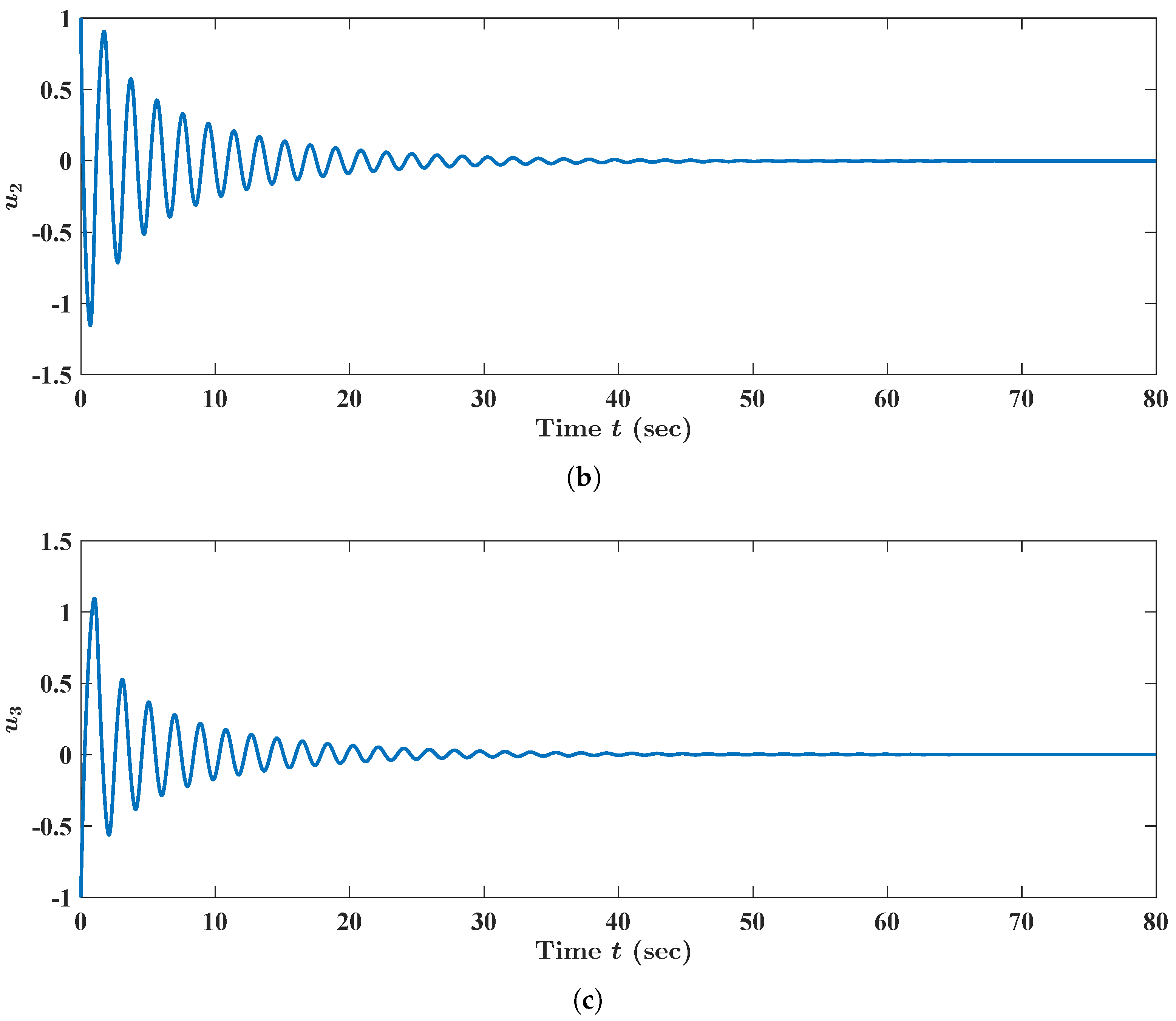
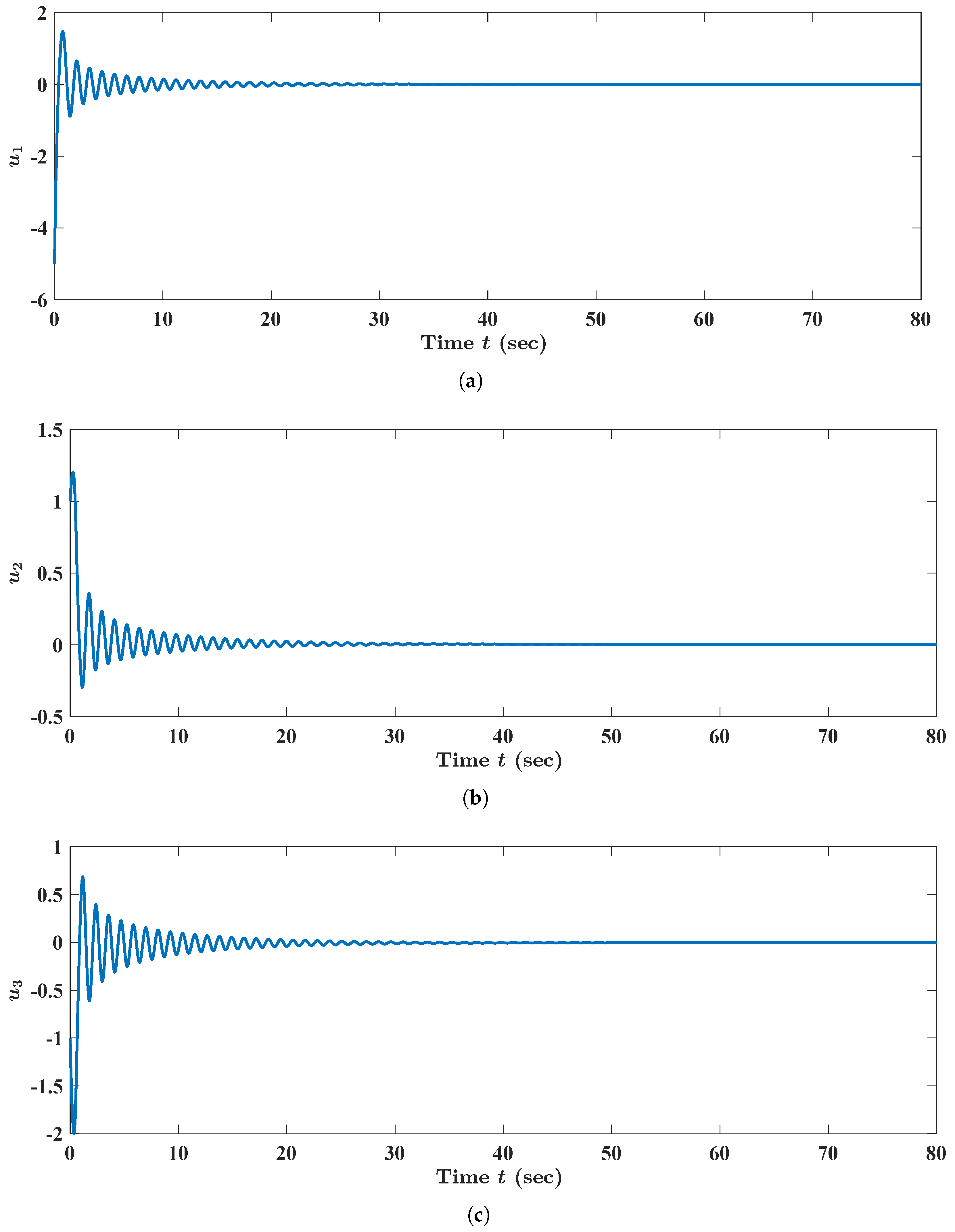
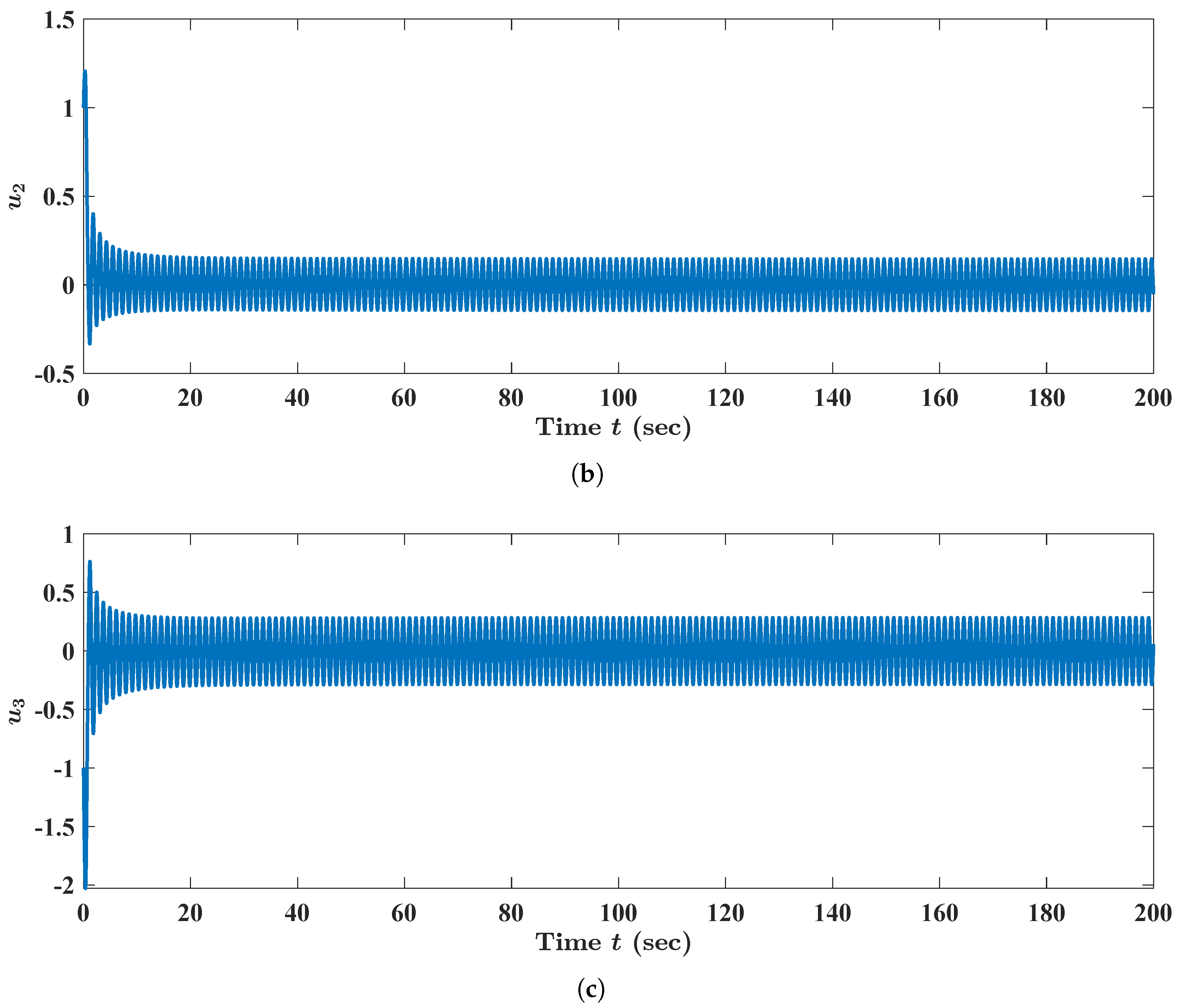
We visualize here the aforementioned Hopf bifurcation phenomenon in FBAMNN (118) with . For this purpose, based on MATLAB, we fixed , as well as , to numerically compute the state trajectory of FBAMNN (118), which is supplemented by the initial condition
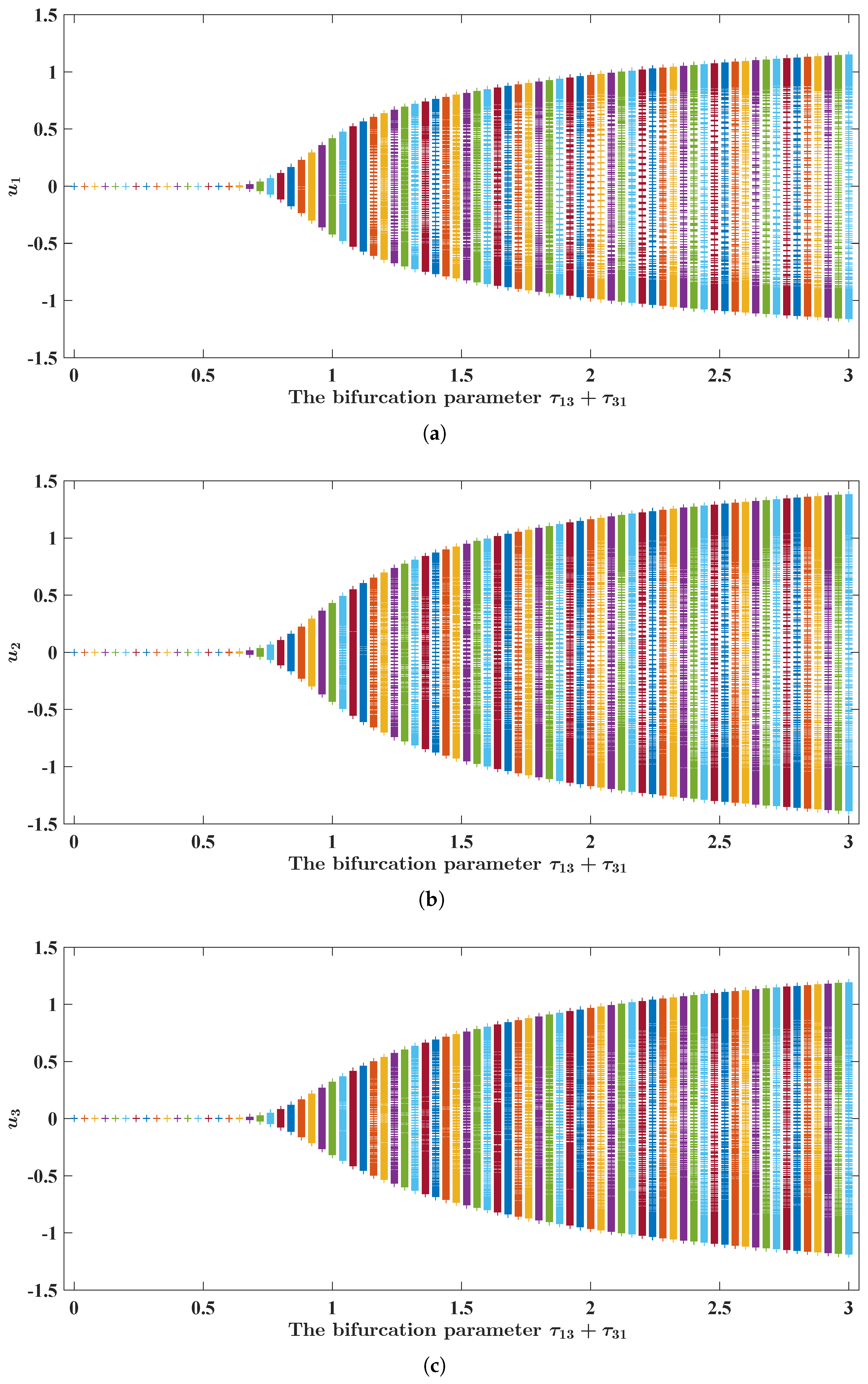
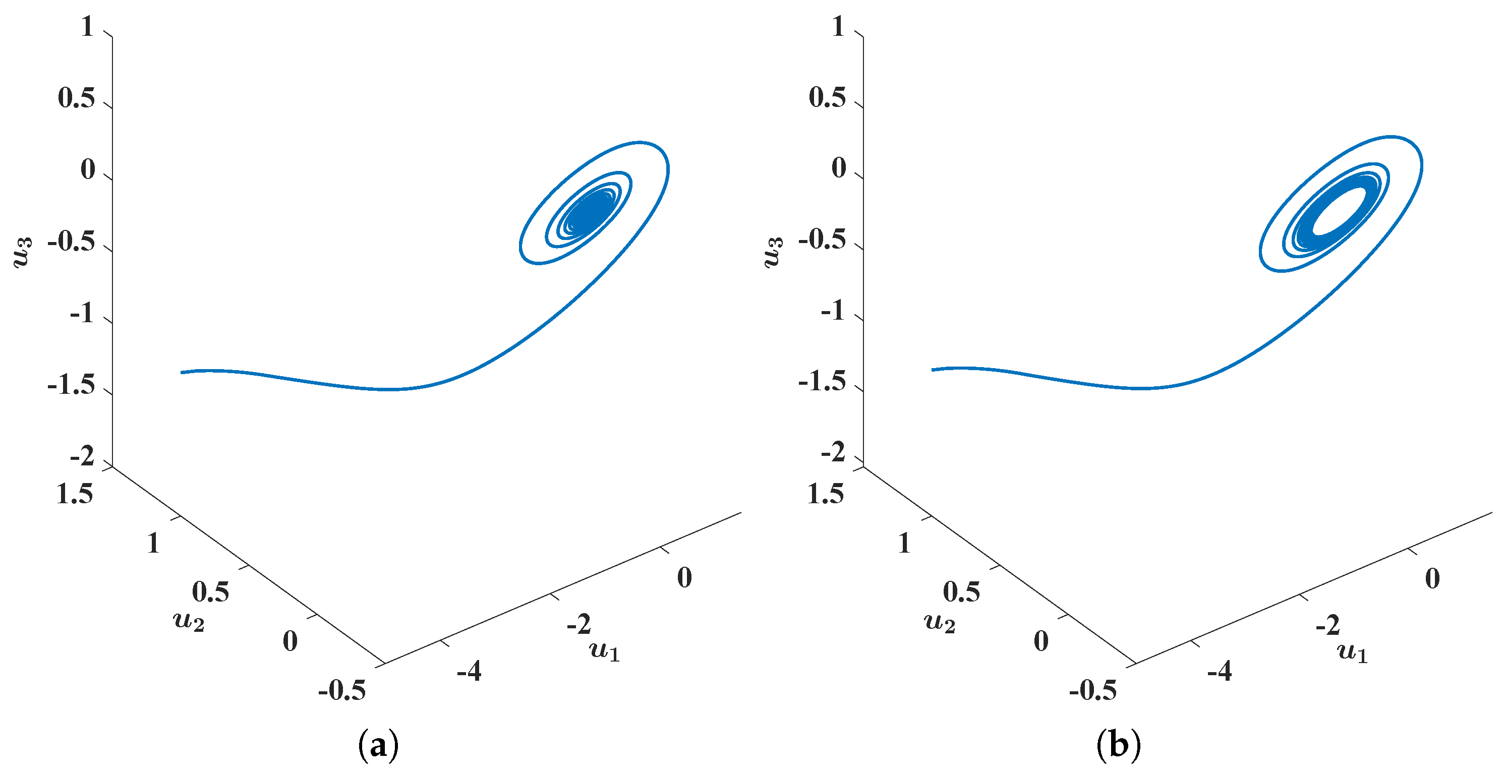
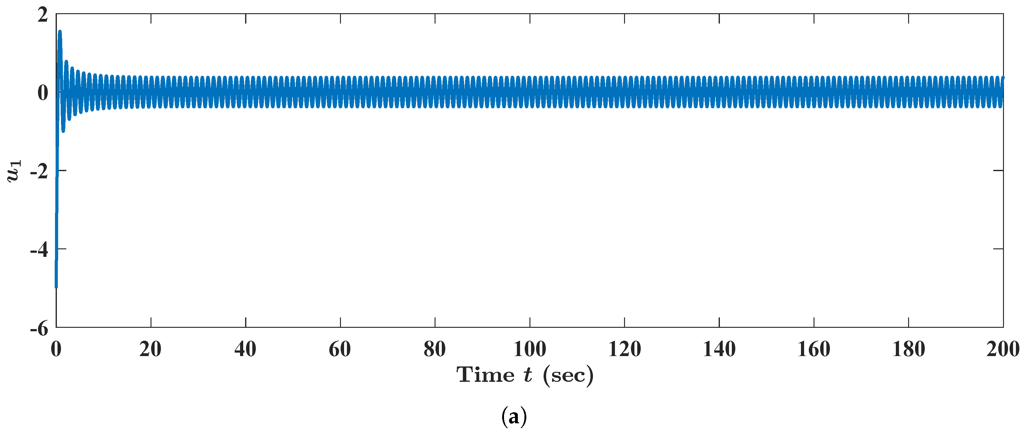
By scrutinizing Figure 1, we can conclude that the state trajectory of FBAMNN (118), with and , tends to the null state trajectory as time t escapes to infinity. We plotted, via MATLAB, the state trajectory of FBAMNN (118), with and in the phase space to obtain Figure 2a; we also found that the state trajectory approached the equilibrium state in the phase space as time t tended to infinity. On the other hand, we fixed , as well as , which we numerically computed, based on MATLAB, the state trajectory of FBAMNN (118), which was supplemented by the initial Condition (120). Through viewing Figure 3, we concluded that the state trajectory of FBAMNN (118), with and , tended to a periodic state trajectory as time t approached infinity. We plotted, via MATLAB, the state trajectory of FBAMNN (118), with and in the phase space to obtain Figure 2b; in addition, we found that the state trajectory approached a non-trivial closed curve in the phase space as time t went to infinity. To display more clearly the existence of the periodic state trajectory in FBAMNN (118), with , we plotted—based on MATLAB—the state trajectory of FBAMNN (118), with and , in the phase space to obtain Figure 4; in this figure, we can see more clearly the existence of the periodic state trajectory in FBAMNN (118) with ). In Figure 5, Figure 6 and Figure 7, we found that a Hopf bifurcation occurred at the point in the FBAMNN detailed in Example 1 (that is, FBAMNN (118) with ).
Example 2.
Let , as well as the constants and that were given in the closed half interval . We perform here some bifurcation analyses of the following FBAMNN
It is evident that is an equilibrium state of FBAMNN (121). As with FBAMNN (118), we linearized FBAMNN (121) at the equilibrium state to obtain
where the time delay and satisfy .
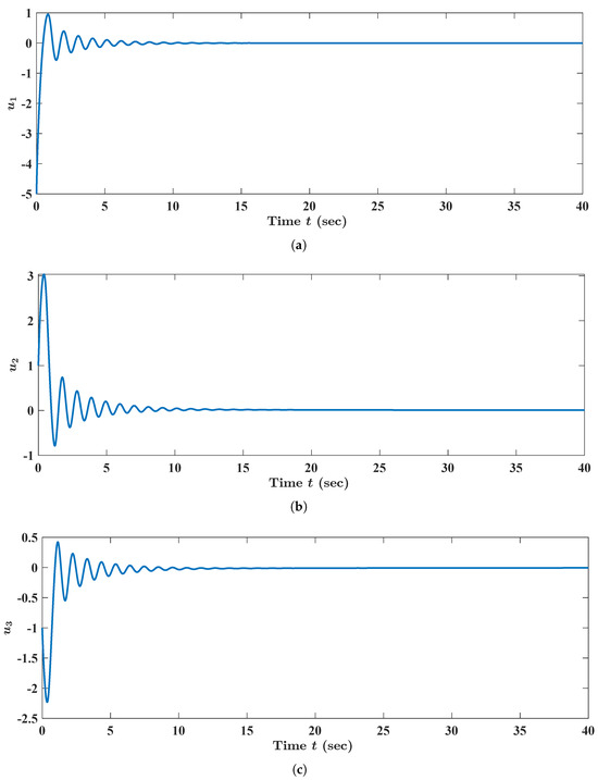
Figure 1.
Numerical and graphical illustrations of the stability of equilibrium states of FBAMNN (4) with and with , which are viewed as the bifurcation parameter and are strictly less than a threshold constant. In addition, is the (unique) state trajectory triplet of FBAMNN (118), with (in actuality, ), which is strictly less than the threshold constant (namely the bifurcation point) . This is approximately equal to , with , such that the initial Condition (120) is satisfied. Equivalently, it could such that it holds that is for all ,, as well as for all and . The graph (curve) of the function , which is the first component of the aforementioned state trajectory triplet , , is plotted in (a). The graph (curve) of the function , which is the second component of the aforementioned state trajectory triplet , , is plotted in (b). The graph (curve) of the function , which is the third component of the aforementioned state trajectory triplet , , is plotted in (c).
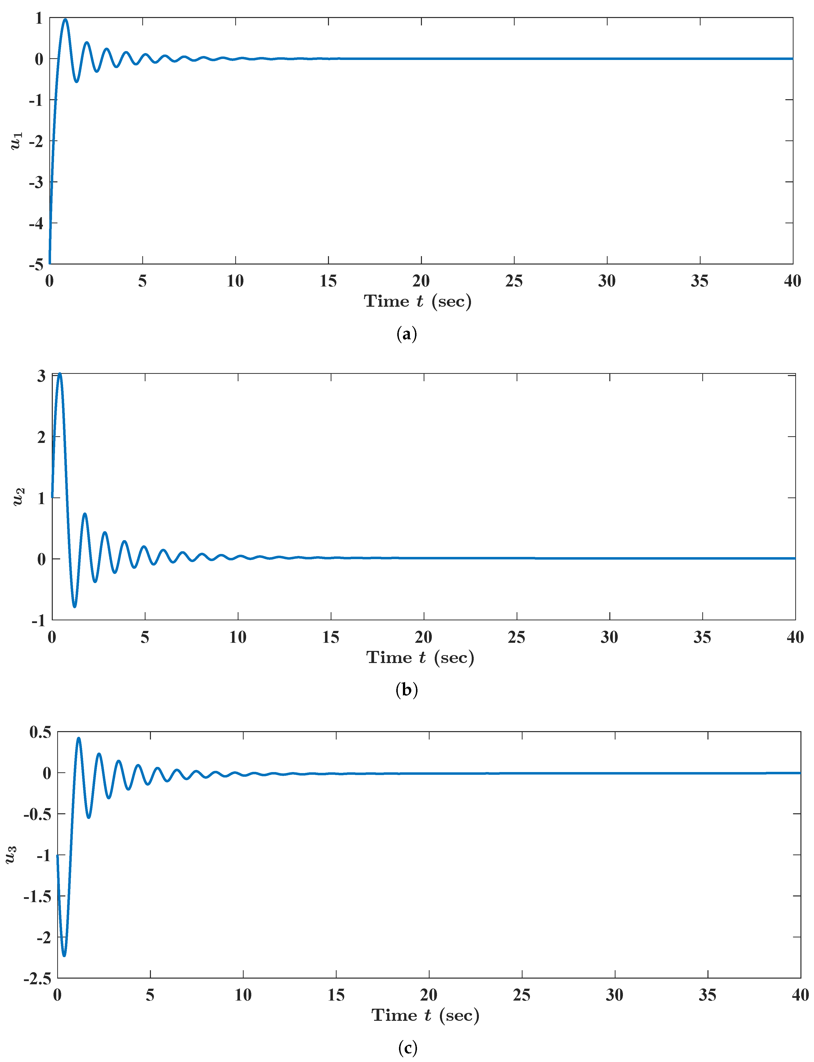
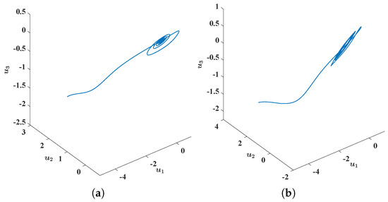
Figure 2.
Numerical and graphical illustrations of FBAMNN (4) with , which undergoes Hopf bifurcation at . In (a), it is plotted that the graph (a parameterized space curve) of the (unique) state trajectory triplet of FBAMNN (118), with (in actuality, ), is strictly less than the threshold constant (namely the bifurcation point) , which is approximately equal to and , such that the initial Condition (120) is satisfied. Equivalently, it could be such that it holds that is for all , and that is for all and . In (b), it is plotted that the graph (a parameterized space curve) of the (unique) state trajectory triplet of FBAMNN (118), with (in actuality, ), is strictly greater than the threshold constant (namely the bifurcation point) , which is approximately equal to and , such that the initial condition (120) is satisfied. Equivalently, it could such that it holds that is for all , and that is for all and .
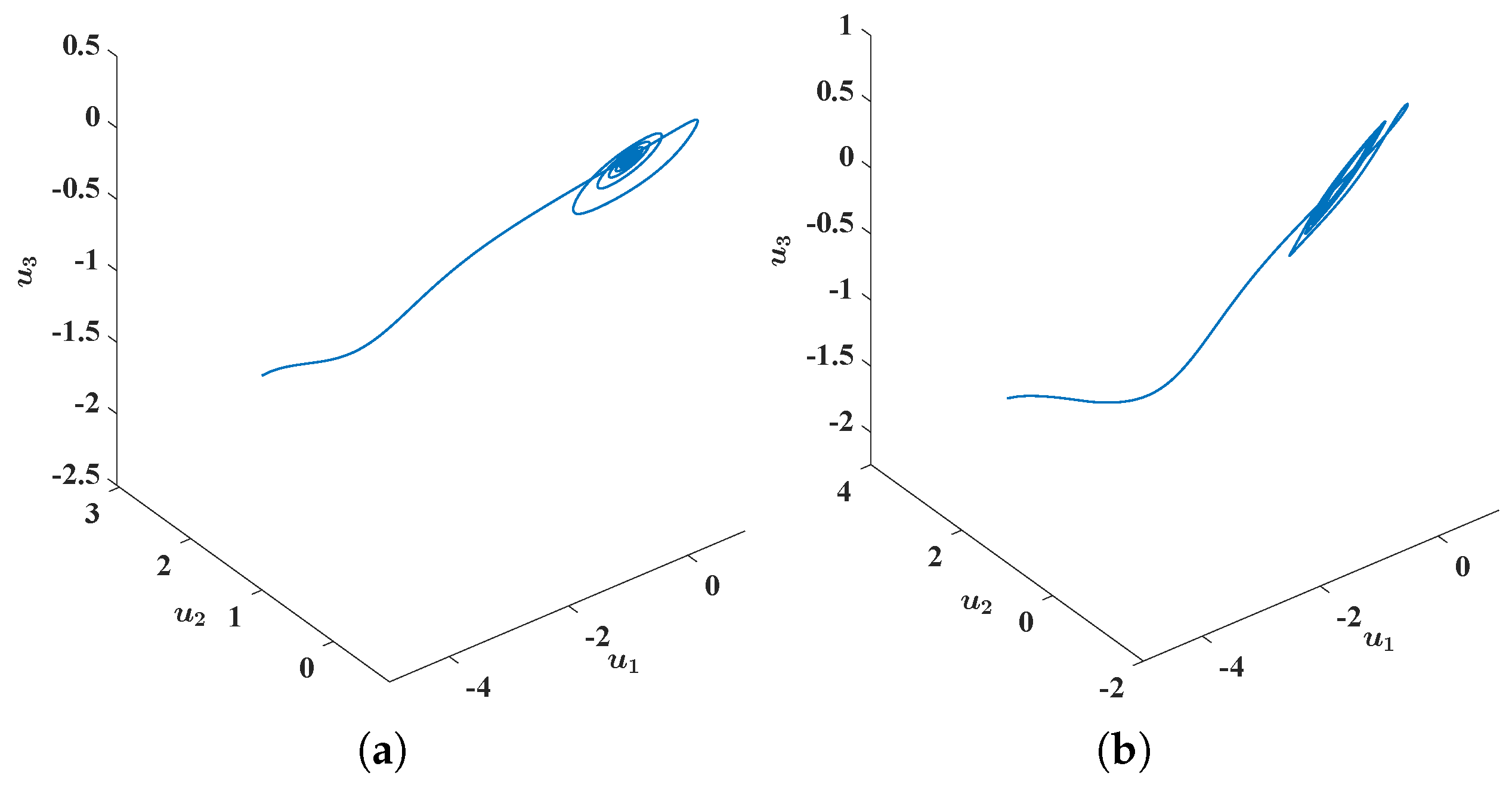
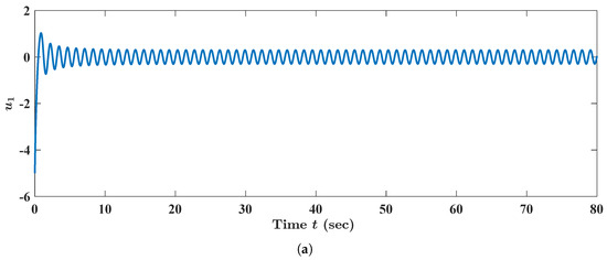
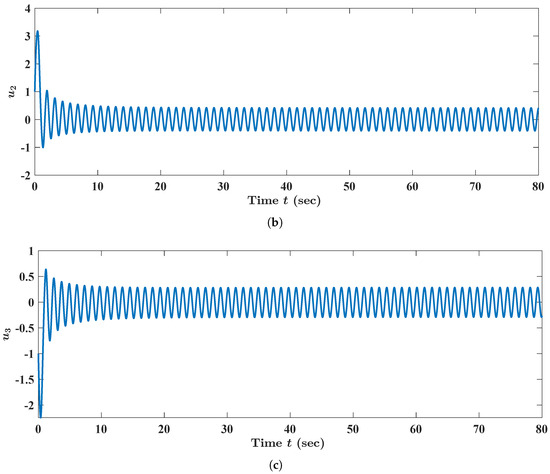
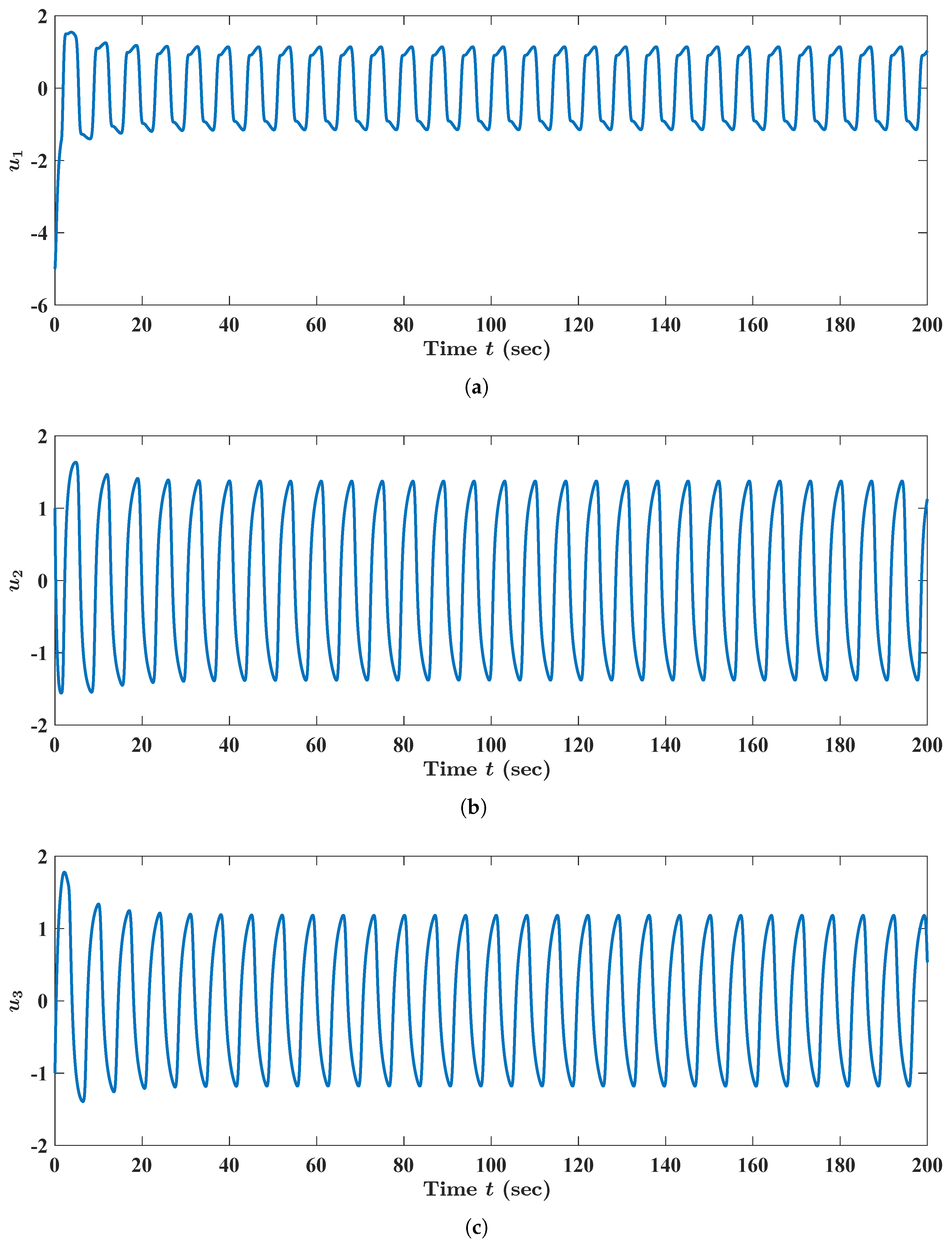
Figure 3.
Numerical and graphical illustrations of the existence and the (asymptotical) stability of the periodic state trajectories of FBAMNN (4) with and with , where the bifurcation parameter is strictly greater than a threshold constant and is opposed to Figure 1. As with Figure 1, is the (unique) state trajectory triplet of FBAMNN (118), with (in actuality, ), which is strictly greater than the threshold constant (namely the bifurcation point) . This is approximately equal to and , such that the initial Condition (120) is satisfied. Equivalently, it could be such that it holds that for all , and that is for all and . The graph (curve) of the function , which is the first component of the aforementioned state trajectory triplet , , is plotted in (a). The graph (curve) of the function , which is the second component of the aforementioned state trajectory triplet , , is plotted in (b). The graph (curve) of the function , which is the third component of the aforementioned state trajectory triplet , , is plotted in (c).
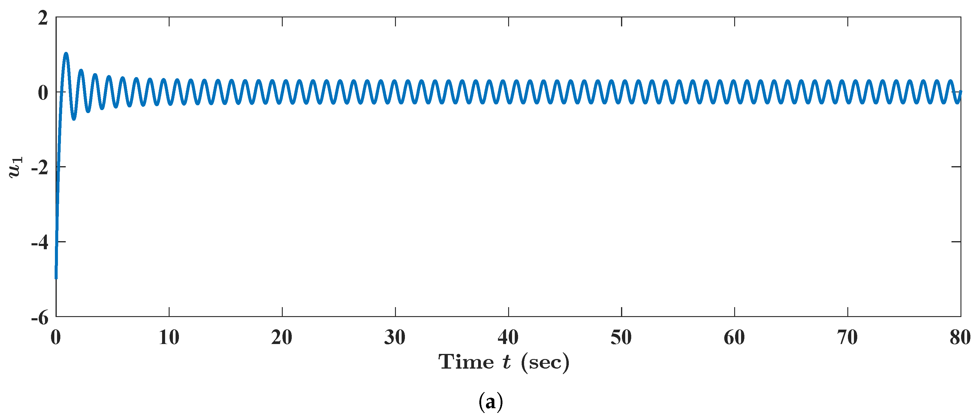
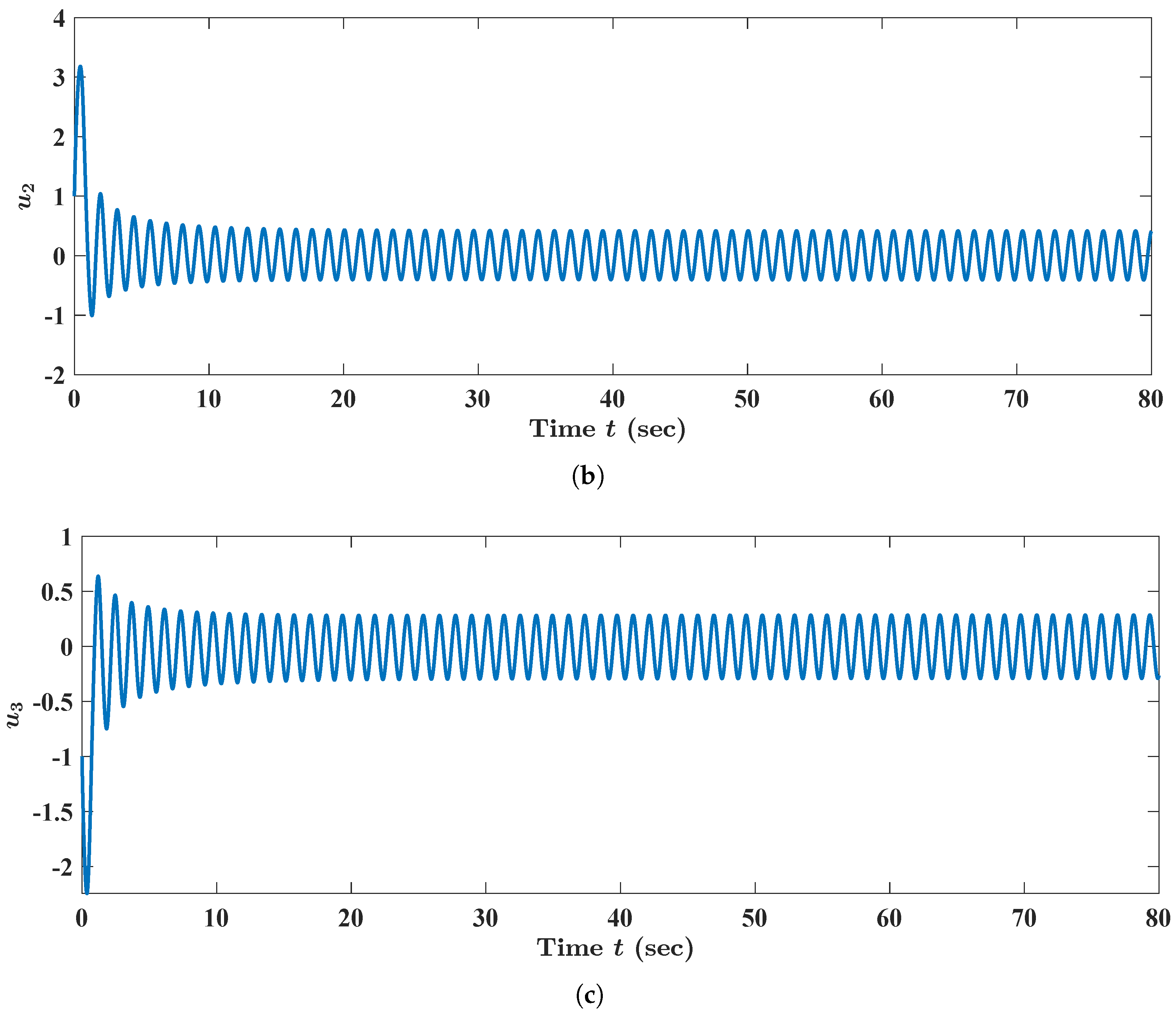
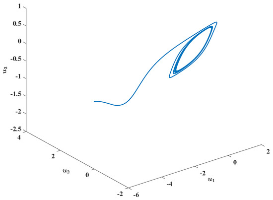
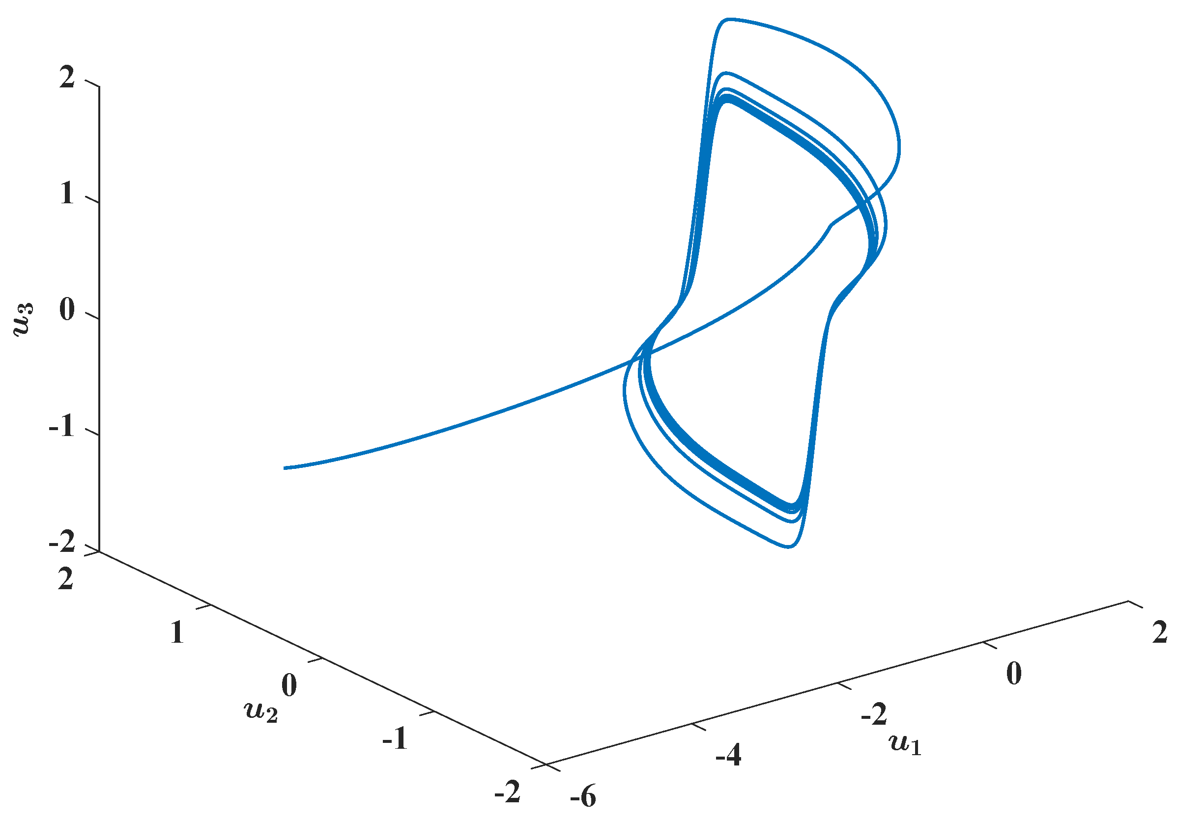
Figure 4.
Numerical and graphical illustration of the existence and the (asymptotical) stability of periodic state trajectories of FBAMNN (4), with and , where the bifurcation parameter is strictly greater than a threshold constant. In Figure 4, it is plotted in the phase space that the graph (which shows a parameterized space curve) of the (unique) state trajectory triplet of FBAMNN (118), with (in actuality, ), is strictly greater than the threshold constant (namely the bifurcation point) , which is approximately equal to and , such that the initial condition (120) is satisfied. Equivalently, it could be such that it holds that is for all , and that is for all and .

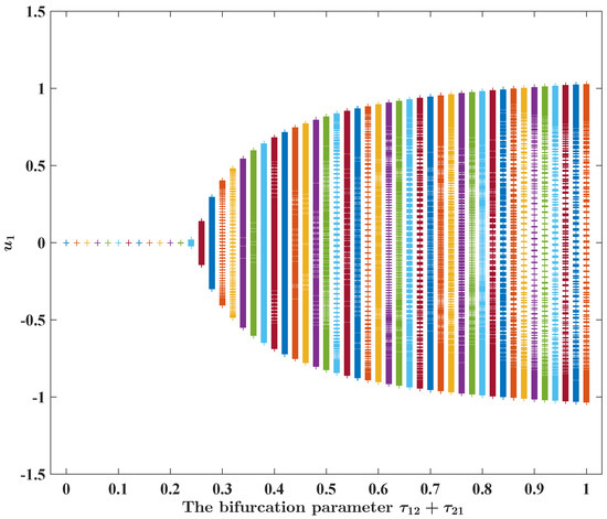
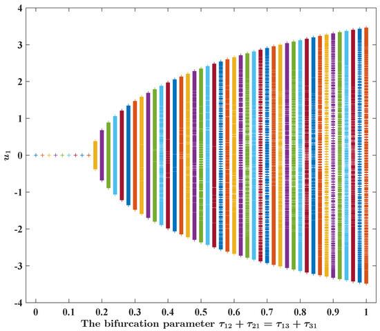
Figure 5.
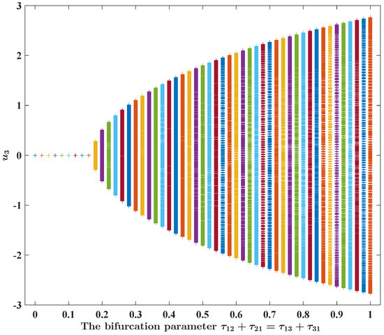
Numerical and graphical illustration of FBAMNN (4), with , which undergoes Hopf bifurcation at . In Figure 5, it is plotted that the bifurcation diagram of FBAMNN (118), with and , is the bifurcation parameter in terms of the component.
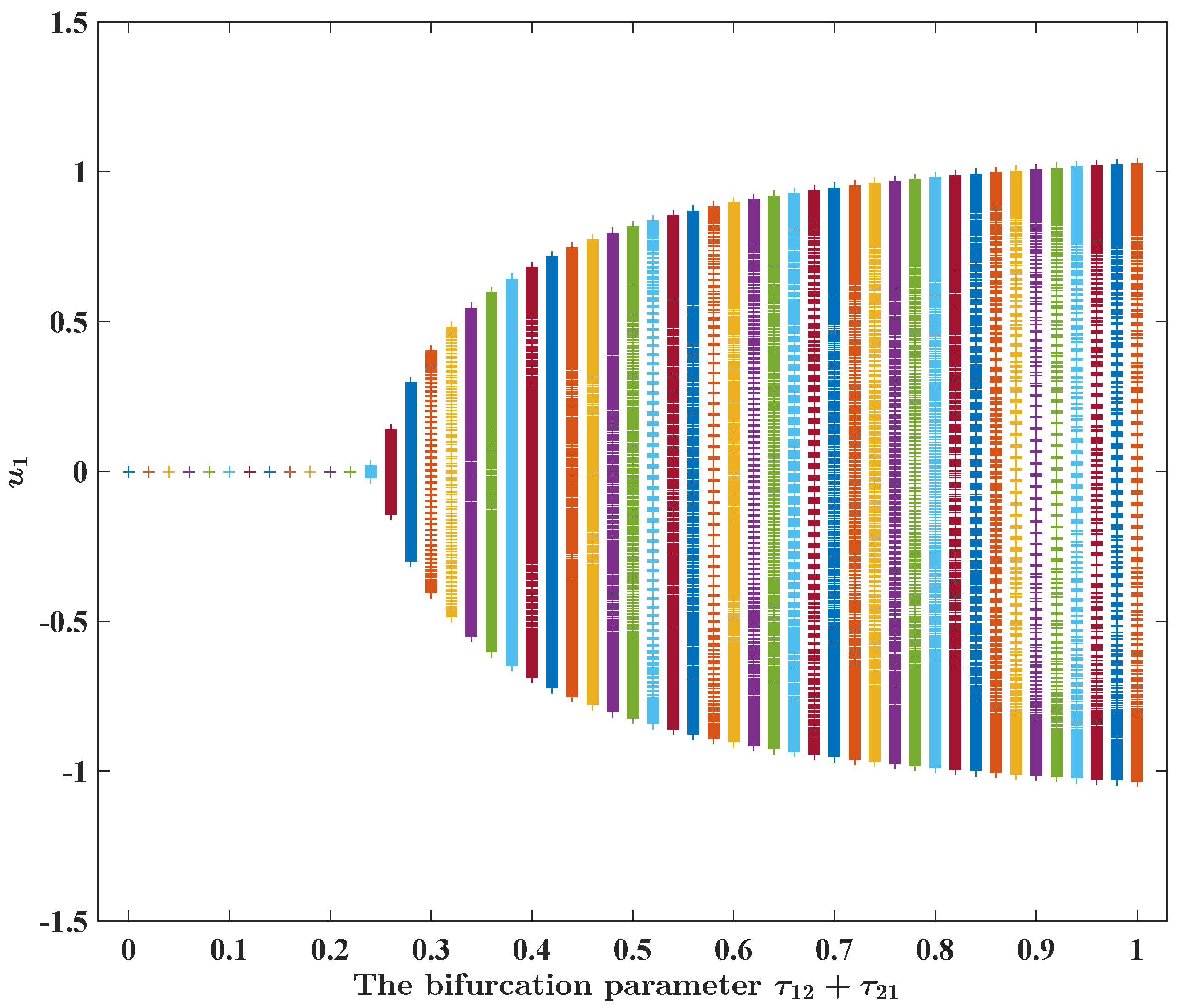
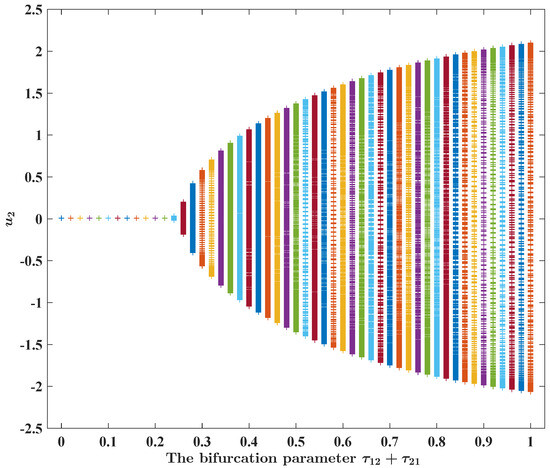
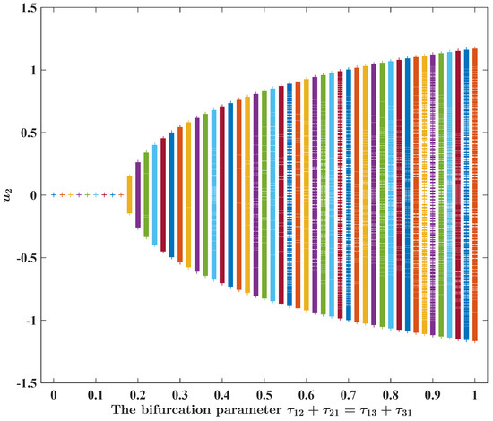
Figure 6.
Numerical and graphical illustration of FBAMNN (4), with , which undergoes Hopf bifurcation at . In Figure 6, it is plotted that the bifurcation diagram of FBAMNN (118), with and , is the bifurcation parameter in terms of the component.
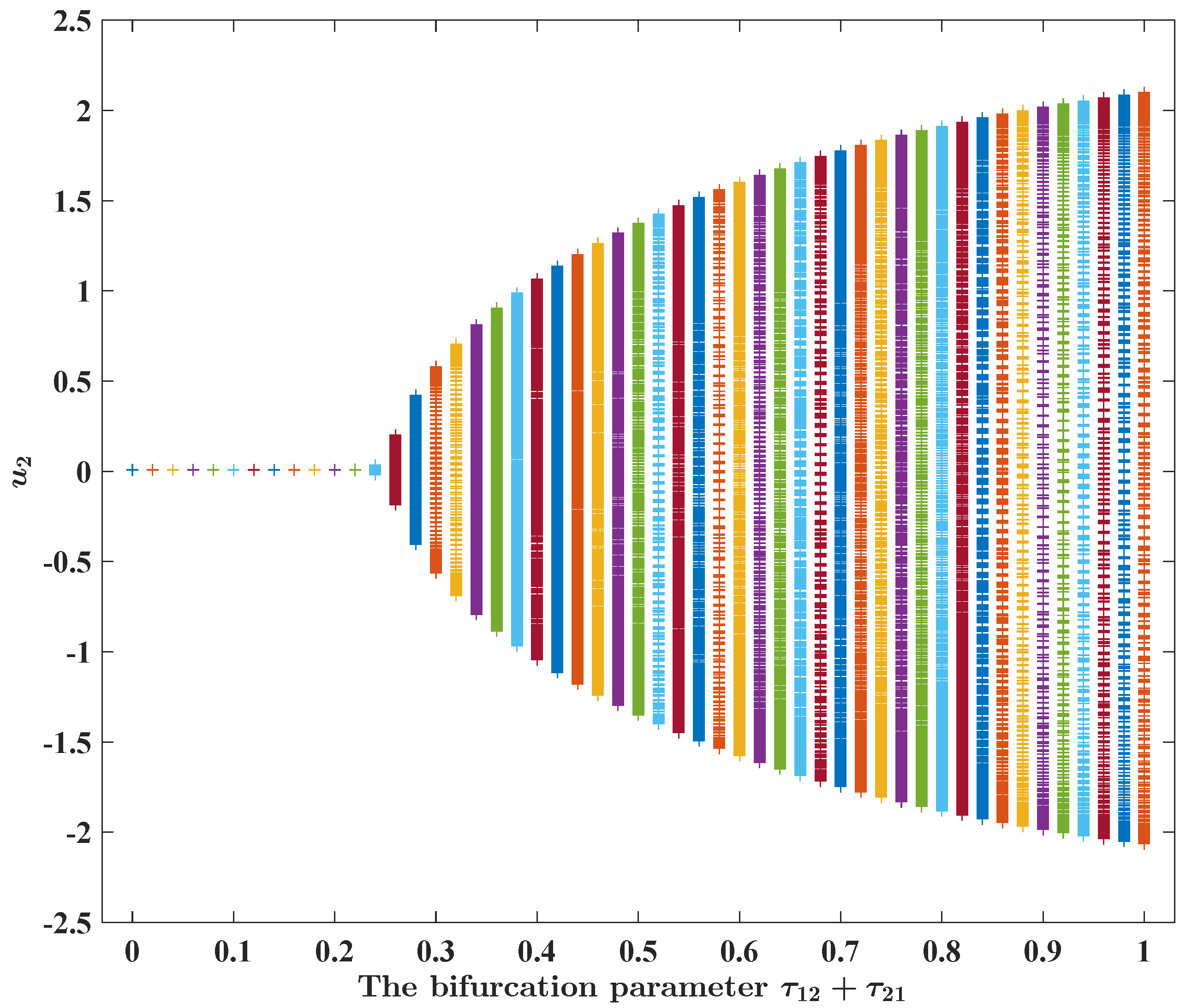
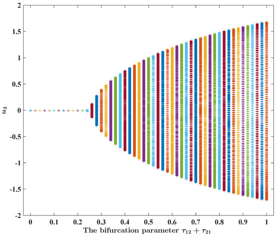
Figure 7.
Numerical and graphical illustration of FBAMNN (4), with , which undergoes Hopf bifurcation at . In Figure 7, it is plotted that the bifurcation diagram of FBAMNN (118), with and , is the bifurcation parameter in terms of the component.

We analyzed FBAMNN (121) (with ), as well as the linearized FBAMNN (122) (with ), to conclude that there exists a positive constant (which is approximately equal to and was numerically calculated via MATLAB) such that the following applies: If and , then the equilibrium state of FBAMNN (121) is (at least locally) asymptotically stable; if , FBAMNN (121), is involved with the parameters and , it undergoes Hopf bifurcation at point .
We visualize here the aforementioned Hopf bifurcation phenomenon in FBAMNN (121) (with ). For this purpose, we fixed , as well as , and we numerically computed, based on MATLAB, the state trajectory of FBAMNN (121), which was supplemented by the initial condition
By carefully examining Figure 8, we concluded that the state trajectory of FBAMNN (121) (with and ) tended to the null state trajectory as time t escaped to infinity. We plotted, via MATLAB, the state trajectory of FBAMNN (121) (with and ) in the phase space to obtain Figure 9; we found that the state trajectory approached the equilibrium state in the phase space as time t tended to infinity. On the other hand, we fixed , as well as , and numerically computed, based on MATLAB, the state trajectory of FBAMNN (121), which was supplemented by the initial Condition (123). By viewing Figure 10, we concluded that the state trajectory (with and ) tended to a periodic state trajectory as time t approached infinity. We plotted, via MATLAB, the state trajectory of FBAMNN (121) (with and ) in the phase space to obtain Figure 11; we found that the state trajectory approached a non-trivial closed curve in the phase space as time t went to infinity. In Figure 12, we found that a Hopf bifurcation occurred at point in the FBAMNN in Example 2 (that is, FBAMNN (121) with ).
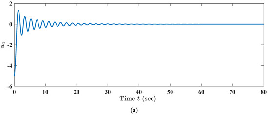
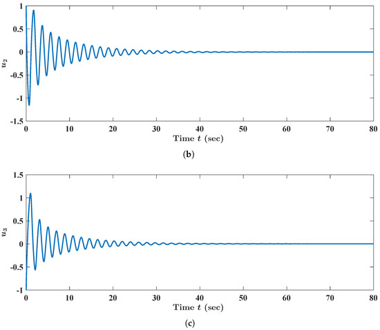
Figure 8.
Numerical and graphical illustrations of the stability of the equilibrium states of FBAMNN (4), with and , which is viewed as the bifurcation parameter and is strictly less than a threshold constant. In addition, is the (unique) state trajectory triplet of FBAMNN (121), with (in actuality, ), which is strictly less than the threshold constant (namely the bifurcation point) . This is approximately equal to and , such that the initial Condition (123) is satisfied. Equivalently, it could be such that it holds that is for all , and that and are for all . The graph (curve) of the function is the first component of the aforementioned state trajectory triplet , , which is plotted in (a). The graph (curve) of the function , which is the second component of the aforementioned state trajectory triplet , , is plotted in (b). The graph (curve) of the function , which is the third component of the aforementioned state trajectory triplet , that is is plotted in (c).
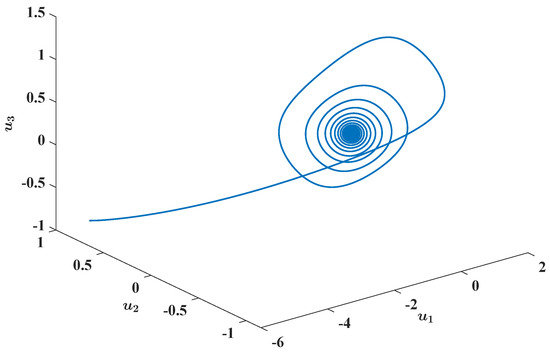
Figure 9.
Numerical and graphical illustration of the stability of equilibrium states of FBAMNN (4) with and , which is viewed as the bifurcation parameter and is strictly less than a threshold constant. In Figure 9, it is plotted in the phase space that the graph (a parameterized space curve) of the (unique) state trajectory triplet of FBAMNN (121), with (in actuality, ), is strictly less than the threshold constant (namely the bifurcation point) . This is approximately equal to and , such that the initial Condition (123) is satisfied. Equivalently, it could be such that it holds that is for all , and that and are for all .
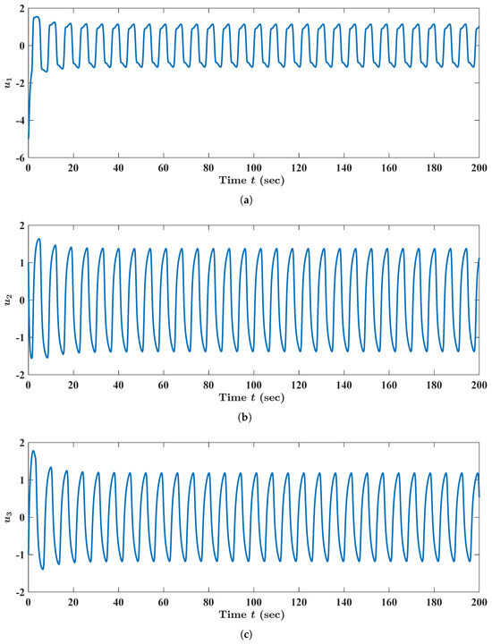
Figure 10.
Numerical and graphical illustration of the existence and the (asymptotical) stability of the periodic state trajectories of FBAMNN (4), with and , which is the bifurcation parameter and is strictly greater than a threshold constant, as opposed to Figure 8. As with Figure 8, is the (unique) state trajectory triplet of FBAMNN (121), with (in actuality, ), which is strictly greater than the threshold constant (namely the bifurcation point) . This is approximately equal to and , such that the initial Condition (123) is satisfied. Equivalently, it could be such that it holds that is for all , and that and are for all . The graph (curve) of the function , which is the first component of the aforementioned state trajectory triplet , is plotted in (a). The graph (curve) of the function , which is the second component of the aforementioned state trajectory triplet , is plotted in (b). The graph (curve) of the function , which is the third component of the aforementioned state trajectory triplet , is plotted in (c).
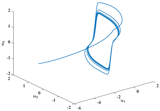
Figure 11.
Numerical and graphical illustration of the existence and the (asymptotical) stability of the periodic state trajectories of FBAMNN (4), with and with , which is the bifurcation parameter and is strictly greater than a threshold constant. In Figure 11, it is plotted in the phase space that the graph (a parameterized space curve) of the (unique) state trajectory triplet of FBAMNN (121), with (in actuality, ), is strictly greater than the threshold constant (namely the bifurcation point) . This is approximately equal to and , such that the initial Condition (123) is satisfied. Equivalently, it could be such that it holds that is for all , and that and are for all .
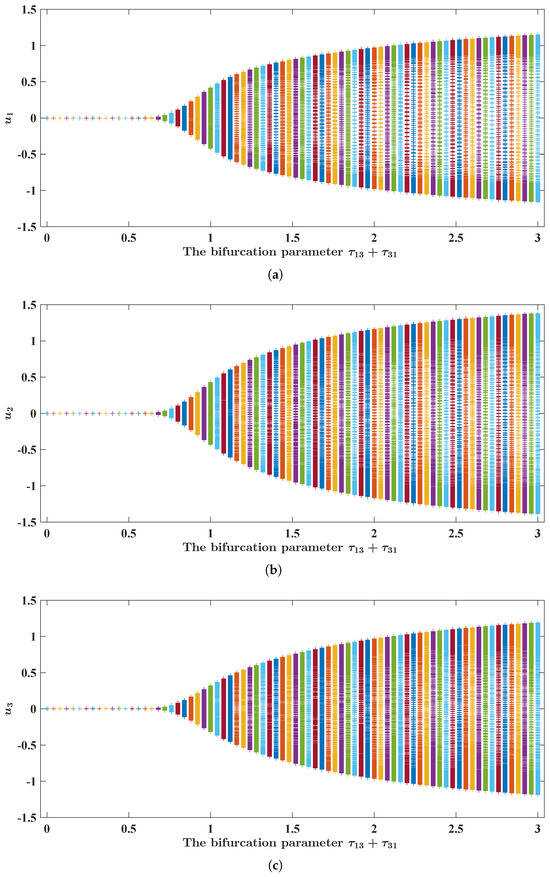
Figure 12.
Numerical and graphical illustrations of FBAMNN (4), with , which underwent Hopf bifurcation at . In (a), it was plotted that the bifurcation diagram of FBAMNN (121), with and , was the bifurcation parameter in terms of the component. In (b), it was plotted that the bifurcation diagram of FBAMNN (121), with and , was the bifurcation parameter in terms of the component. In (c), it was plotted that the bifurcation diagram of FBAMNN (121), with and , was the bifurcation parameter in terms of the component.
Example 3.
Let the constants , , , and be given in the closed half interval , such that . We perform here some bifurcation analyses of the following FBAMNN equation:
It is evident that is an equilibrium state of FBAMNN (124). As with FBAMNNs (118) and (121), we linearized FBAMNN (124) at the equilibrium state to obtain
in which the time delay , , , and satisfy .
We analyzed FBAMNN (124), as well as the linearized FBAMNN (125), to conclude that there exists a positive constant (which is approximately equal to and was numerically calculated via MATLAB), such that the following applies: If , then the equilibrium state of FBAMNN (124) is (at least locally) asymptotically stable; moreover, FBAMNN (124) undergoes Hopf bifurcation at point .
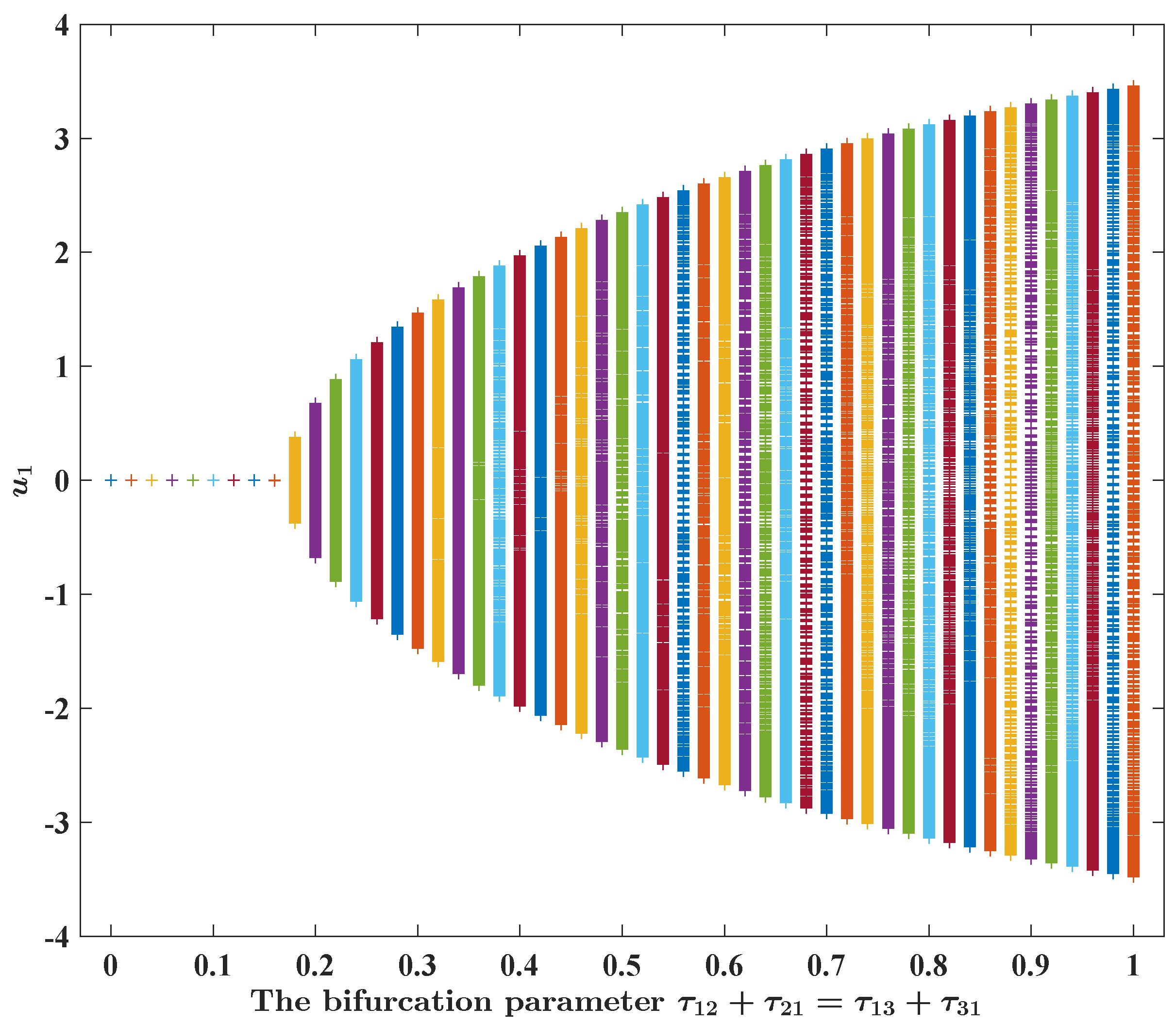
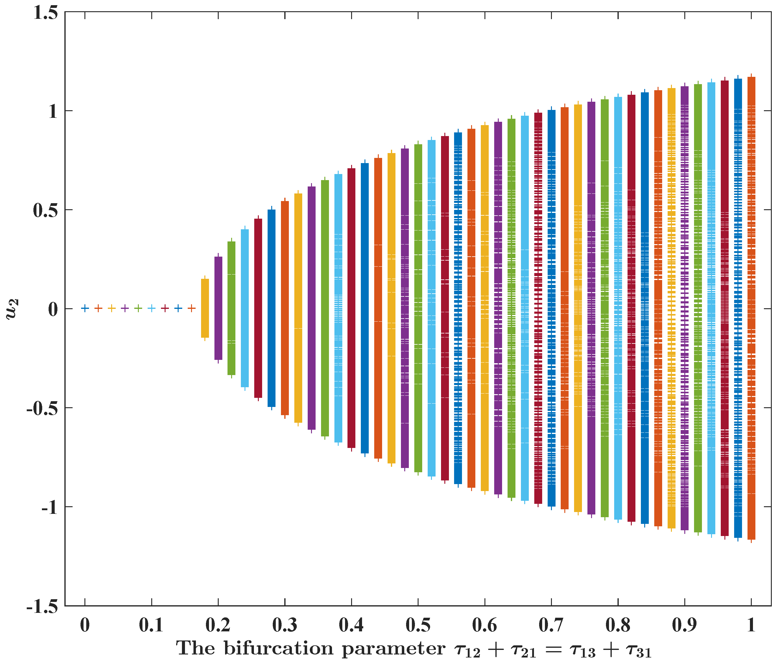
We visualize here the aforementioned Hopf bifurcation phenomenon in FBAMNN (124) (with ). For this purpose, we fixed , as well as numerically computed, based on MATLAB, the state trajectory of FBAMNN (124), which was supplemented by the initial condition
By viewing Figure 13, we concluded that the state trajectory of FBAMNN (124) () tended to the null state trajectory as time t escaped to infinity. We plotted, via MATLAB, the state trajectory of FBAMNN (124) (with ) in the phase space to obtain Figure 14a; we found that the state trajectory approached the equilibrium state in the phase space as time t tended to infinity. On the other hand, we fixed and numerically computed, based on MATLAB, the state trajectory of FBAMNN (124), which was supplemented by the initial condition (126). By viewing Figure 15, we concluded that the state trajectory of FBAMNN (124) (with ) tended to a periodic state trajectory as time t approached infinity. We plotted, via MATLAB, the state trajectory of FBAMNN (118) (with ) in the phase space to obtain Figure 14b; we found that the state trajectory approached a non-trivial closed curve in the phase space as time t went to infinity. In Figure 16, Figure 17 and Figure 18, we found that a Hopf bifurcation occurred at the point in the FBAMNN equation in Example 3 (that is, FBAMNN (124) with ).
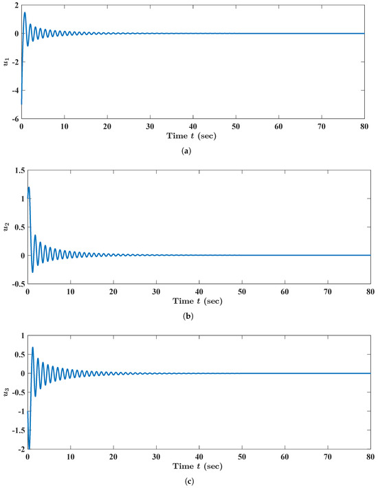
Figure 13.
Numerical and graphical illustrations of the stability of the equilibrium states of FBAMNN (4), with , which is viewed as the bifurcation parameter and is strictly less than a threshold constant. In addition, is the (unique) state trajectory triplet of FBAMNN (124), with (in actuality, ), which is strictly less than the threshold constant (the bifurcation point) . This is approximately equal to , such that the initial Condition (126) is satisfied. Equivalently, it could be such that it holds that is for all , is for all , and that is for all . The graph (curve) of the function is the first component of the aforementioned state trajectory triplet , , which is plotted in (a). The graph (curve) of the function , which is the second component of the aforementioned state trajectory triplet , , is plotted in (b). The graph (curve) of the function , which is the third component of the aforementioned state trajectory triplet , is plotted in (c).

Figure 14.
Numerical and graphical illustration of FBAMNN (4), which underwent Hopf bifurcation at . In (a), it is plotted that the graph (which is a parameterized space curve) of the (unique) state trajectory triplet of FBAMNN (118), with (in actuality, ), is strictly less than the threshold constant (namely the bifurcation point) . This is approximately equal to , such that the initial Condition (126) is satisfied. Equivalently, it could be such that it holds that is for all , is for all , and that is for all . In (b), it is plotted that the graph (which is a parameterized space curve) of the (unique) state trajectory triplet of FBAMNN (118), with (in actuality, ) is strictly greater than the threshold constant (namely the bifurcation point) . This is approximately equal to , such that the initial Condition (126) is satisfied. Equivalently, it could be such that it holds that is for all , is for all , and that is for all .

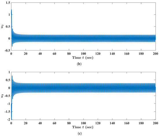
Figure 15.
Numerical and graphical illustrations of the existence and (asymptotic) stability of the periodic state trajectories of FBAMNN (4), with , which is the bifurcation parameter and is strictly greater than a threshold constant, as opposed to Figure 13. As with Figure 13, is the (unique) state trajectory triplet of FBAMNN (124), with (in actuality, ), and it is strictly greater than the threshold constant (namely the bifurcation point) . This is approximately equal to , such that the initial Condition (126) is satisfied. Equivalently, it could be such that it holds that is for all , is for all , and is for all . The graph (curve) of the function , which is the first component of the aforementioned state trajectory triplet , is plotted in (a). The graph (curve) of the function , which is the second component of the aforementioned state trajectory triplet , is plotted in (b). The graph (curve) of the function , which is the third component of the aforementioned state trajectory triplet , is plotted in (c).
5. Concluding Remarks
In this paper, we conducted a relatively systematic and intensive analysis on the influence of delays on the dynamics of a class of time-delayed non-commensurate Caputo FBAMNNs composed of three neurons. Via a standard (Banach’s) fixed-point argument, we obtained the existence and uniqueness of the state trajectories of the FBAMNNs dealt with in this paper, i.e., FBAMNN (4) (see Theorem 1 in Section 3 for the details). By borrowing ideas from [23,31,44], we found that one can prove the ultimate boundedness of state the trajectories of FBAMNN (4); in addition, we also pointed out that one can provide a unified treatment of the state trajectories of FBAMNN (4) when proving that, when under two situations, either all of its (discrete) delays are positive or that some of the delays vanish. This was achieved with an appeal to Duhamel’s principle for Caputo fractional-differential-type equations (see Remark 2 in Section 3 for the details). By applying ideas and techniques that are analogous to those that were frequently utilized in References [23,31,44], and which were based on the idea of linearization, we analyzed the stability and bifurcation phenomenon (the Hopf bifurcation, more precisely) of FBAMNN (4) (see Theorems 2–4 in Section 3 for the details). Our obtained results revealed that the large time delays in FBAMNNs can lead to complex dynamics such as the bifurcation phenomenon. In addition, these theoretical results allowed us to design a (feedback) control to attenuate or to even remove the bifurcation phenomenon of FBAMNNs.
Author Contributions
Conceptualization, C.W., X.Z. and Z.L.; methodology, C.W., X.Z. and Z.L.; software, C.W. and Q.M.; validation, C.W., X.Z. and Z.L.; formal analysis, C.W. and Q.M.; investigation, C.W. and X.Z.; resources, C.W. and Q.M.; writing—original draft preparation, C.W.; writing—review and editing, C.W., X.Z. and Z.L.; visualization, C.W., X.Z., Q.M. and Z.L.; supervision, X.Z. and Z.L.; project administration, C.W.; funding acquisition, C.W. All authors have read and agreed to the published version of the manuscript.
Funding
Chengqiang Wang was partially supported by the Startup Foundation for Newly Recruited Employees from the Xichu Talents Foundation of Suqian University (#2022XRC033); the Guiding Science and Technology Planning Program of Suqian (#Z2023131); the Excellent Graduation Design (Thesis) Fostering Program of Suqian University (2023YXBYSJ05); the Professional Certification Oriented Teaching Reform Research Special Program of Suqian University; the Innovation and Entrepreneurship Education Reform Research Program of Suqian University (#2023cxcy08); the NSFC (#11701050); the Qing Lan Project of Jiangsu; the ‘High Quality Public Course Teaching Reform’ Special Program for colleges and universities of Jiangsu (#2022JDKT106); the Higher Education Reform Research Project of Jiangsu (#2023JSJG718); and the Higher Education Scientific Research Planning Project of the Higher Education Association of China (#23SX0203).
Data Availability Statement
No new data were created or analyzed in this study.
Conflicts of Interest
The authors declare that they have no conflicts of interest.
References
- Cohen, M.A.; Grossberg, S. Adaptive bidirectional associative memories. IEEE Trans. Syst. Man, Cybern. 1983, 26, 815–826. [Google Scholar] [CrossRef]
- Kosko, B. Adaptive bidirectional associative memories. Appl. Opt. 1987, 26, 4947–4960. [Google Scholar] [CrossRef] [PubMed]
- Kosko, B. Bidirectional associative memories. IEEE Trans. Syst. Man Cybern. 1988, 18, 49–60. [Google Scholar] [CrossRef]
- Liu, Y.; Wang, Z.; Liu, X. Global exponential stability of generalized recurrent neural networks with discrete and distributed delays. Neural Netw. 2006, 19, 667–675. [Google Scholar] [CrossRef] [PubMed]
- Liu, Y.; Wang, Z.; Liu, X. A comprehensive review of stability analysis of continuous-time recurrent neural networks. IEEE Trans. Neural Netw. Learn. Syst. 2014, 25, 1229–1262. [Google Scholar] [CrossRef]
- Gopalsamy, K.; He, X. Delay-independent stability in bidirectional associative memory networks. IEEE Trans. Neural Netw. 1994, 5, 998–1002. [Google Scholar] [CrossRef]
- Park, J.H.; Park, C.H.; Kwon, O.M.; Lee, S.M. A new stability criterion for bidirectional associative memory neural networks of neutral-type. Appl. Math. Comput. 2008, 199, 716–722. [Google Scholar] [CrossRef]
- Zhu, Q.; Li, X.; Yang, X. Exponential stability for stochastic reaction–diffusion BAM neural networks with time-varying and distributed delays. Appl. Math. Comput. 2011, 217, 6078–6091. [Google Scholar] [CrossRef]
- Zhu, Q.; Huang, C.; Yang, X. Exponential stability for stochastic jumping BAM neural networks with time-varying and distributed delays. Nonlinear Anal. Hybrid Syst. 2011, 5, 52–77. [Google Scholar] [CrossRef]
- Wang, F.; Wang, C. Mean-square exponential stability of fuzzy stochastic BAM networks with hybrid delays. Adv. Differ. Equ. 2018, 2018, 235. [Google Scholar] [CrossRef]
- Tang, R.; Yang, X.; Wan, X.; Zou, Y.; Cheng, Z.; Fardoun, H.M. Finite-time synchronization of nonidentical BAM discontinuous fuzzy neural networks with delays and impulsive effects via non-chattering quantized control. Commun. Nonlinear Sci. Numer. Simul. 2019, 78, 104893. [Google Scholar] [CrossRef]
- Wang, C.; Zhao, X.; Wang, Y. Finite-time stochastic synchronization of fuzzy bi-directional associative memory neural networks with Markovian switching and mixed time delays via intermittent quantized control. AIMS Math. 2023, 8, 4098–4125. [Google Scholar] [CrossRef]
- Wang, C.; Zhao, X.; Wang, C.; Lv, Z. Synchronization of Takagi–Sugeno fuzzy time-delayed stochastic bidirectional associative memory neural networks driven by Brownian motion in pre-assigned settling time. Mathematics 2023, 11, 3697. [Google Scholar] [CrossRef]
- Wang, C.; Zhao, X.; Zhang, Y.; Lv, Z. Global existence and fixed-time synchronization of a hyperchaotic financial system governed by semi-linear parabolic partial differential equations equipped with the homogeneous Neumann boundary condition. Entropy 2023, 25, 359. [Google Scholar] [CrossRef] [PubMed]
- Gularte, K.H.M.; Gomez, J.C.G.; Rabelo, H.S.; Vargas, J.A.R. Minimal underactuated synchronization with applications to secure communication. Commun. Nonlinear Sci. Numer. Simul. 2023, 125, 107376. [Google Scholar] [CrossRef]
- Wang, C.; Jia, Z.; Zhang, C.; Zhao, X. Almost surely exponential convergence analysis of time delayed uncertain cellular neural networks driven by Liu process via Lyapunov–Krasovskii functional approach. Entropy 2023, 25, 1482. [Google Scholar] [CrossRef] [PubMed]
- Zhou, Y.; Zhang, Y. Noether symmetries for fractional generalized Birkhoffian systems in terms of classical and combined Caputo derivatives. Acta Mech. 2020, 231, 3017–3029. [Google Scholar] [CrossRef]
- Sumelka, W.; Łuczak, B.; Gajewski, T.; Voyiadjis, G.Z. Modelling of AAA in the framework of time-fractional damage hyperelasticity. Int. J. Solids Struct. 2020, 206, 30–42. [Google Scholar] [CrossRef]
- Chen, J.; Xiao, M.; Wu, X.; Wang, Z.; Cao, J. Spatiotemporal dynamics on a class of (n+1)-dimensional reaction–diffusion neural networks with discrete delays and a conical structure. Chaos Solitons Fractals 2022, 164, 112675. [Google Scholar] [CrossRef]
- Li, H.; Zhang, L.; Hu, C.; Jiang, Y.; Teng, Z. Dynamical analysis of a fractional-order predator-prey model incorporating a prey refuge. J. Appl. Math. Comput. 2017, 54, 435–449. [Google Scholar] [CrossRef]
- Xu, C.; Liao, M.; Li, P.; Yuan, S. New insights on bifurcation in a fractional-order delayed competition and cooperation model of two enterprises. J. Appl. Anal. Comput. 2021, 11, 1240–1258. [Google Scholar] [CrossRef]
- Deng, W.; Li, C.; Lü, J. Stability analysis of linear fractional differential system with multiple time delays. Nonlinear Dyn. 2007, 48, 409–416. [Google Scholar] [CrossRef]
- Li, P.; Yan, J.; Xu, C.; Shang, Y. Dynamic analysis and bifurcation study on fractional-order tri-neuron neural networks incorporating delays. Fractal Fract. 2022, 6, 161. [Google Scholar] [CrossRef]
- Xu, C.; Mu, D.; Liu, Z.; Pang, Y.; Liao, M.; Aouiti, C. New insight into bifurcation of fractional-order 4D neural networks incorporating two different time delays. Commun. Nonlinear Sci. Numer. Simul. 2023, 118, 107043. [Google Scholar] [CrossRef]
- Xu, C.; Liu, Z.; Li, P.; Yan, J.; Yao, L. Bifurcation mechanism for fractional-order three-triangle multi-delayed neural networks. Neural Process. Lett. 2022, 55, 6125–6151. [Google Scholar] [CrossRef]
- Xu, C.; Zhang, W.; Liu, Z.; Li, P.; Yao, L. Bifurcation study for fractional-order three-layer neural networks involving four time delays. Cogn. Comput. 2022, 14, 714–732. [Google Scholar] [CrossRef]
- Xu, C.; Liao, M.; Li, P.; Yuan, S. Impact of leakage delay on bifurcation in fractional-order complex-valued neural networks. Chaos Solitons Fractals 2021, 142, 110535. [Google Scholar] [CrossRef]
- Xu, C.; Aouiti, C. Comparative analysis on Hopf bifurcation of integer-order and fractional-order two-neuron neural networks with delay. Int. J. Circuit Theory Appl. 2020, 48, 1459–1475. [Google Scholar] [CrossRef]
- Xu, C.; Mu, D.; Liu, Z.; Pang, Y.; Liao, M.; Li, P.; Yao, L.; Qin, Q. Comparative exploration on bifurcation behavior for integer-order and fractional-order delayed BAM neural networks. Nonlinear Anal. Model. Control. 2022, 27, 1–24. [Google Scholar] [CrossRef]
- Ou, W.; Xu, C.; Cui, Q.; Liu, Z.; Pang, Y.; Farman, M.; Ahmad, S.; Zeb, A. Mathematical study on bifurcation dynamics and control mechanism of tri-neuron bidirectional associative memory neural networks including delay. Math. Methods Appl. Sci. 2023, 54, 435–449. [Google Scholar] [CrossRef]
- Xu, C.; Zhang, W.; Aouiti, C.; Liu, Z.; Yao, L. Further analysis on dynamical properties of fractional-order bi-directional associative memory neural networks involving double delays. Math. Methods Appl. Sci. 2022, 45, 11736–11754. [Google Scholar] [CrossRef]
- Yu, W.; Cao, J. Stability and Hopf bifurcation analysis on a four-neuron BAM neural network with time delays. Phys. Lett. A 2006, 351, 64–78. [Google Scholar] [CrossRef]
- Xu, C.; Zhang, W.; Aouiti, C.; Liu, Z.; Liao, M.; Li, P. Further investigation on bifurcation and their control of fractional-order bidirectional associative memory neural networks involving four neurons and multiple delays. Math. Methods Appl. Sci. 2023, 46, 3091–3114. [Google Scholar] [CrossRef]
- Yang, Y.; Ye, J. Stability and bifurcation in a simplified five-neuron BAM neural network with delays. Chaos Solitons Fractals 2009, 42, 2357–2363. [Google Scholar] [CrossRef]
- Li, P.; Lu, Y.; Xu, C.; Ren, J. Bifurcation phenomenon and control technique in fractional BAM neural network models concerning delays. Fractal Fract. 2022, 7, 7. [Google Scholar] [CrossRef]
- Xu, C.; Aouiti, C.; Liu, Z. A further study on bifurcation for fractional order BAM neural networks with multiple delays. Neurocomputing 2020, 417, 501–515. [Google Scholar] [CrossRef]
- Liu, Y.; Li, S.; Liu, Z.; Wang, R. High codimensional bifurcation analysis to a six-neuron BAM neural network. Cogn. Neurodyn. 2016, 10, 149–164. [Google Scholar] [CrossRef] [PubMed]
- Li, W.; Liao, M.; Li, D.; Xu, C.; Li, B. Dynamic behavior of a class of six-neuron fractional BAM neural networks. Fractal Fract. 2023, 7, 520. [Google Scholar] [CrossRef]
- Huang, C.; Li, N.; Cao, J.; Hayat, T. Dynamical analysis of a delayed six-neuron BAM network. Complexity 2016, 2016, 9–28. [Google Scholar] [CrossRef]
- Xu, C.; Liu, Z.; Yao, L.; Aouiti, C. Further exploration on bifurcation of fractional-order six-neuron bi-directional associative memory neural networks with multi-delays. Appl. Math. Comput. 2021, 410, 126458. [Google Scholar] [CrossRef]
- Li, B.; Liao, M.; Xu, C.; Chen, H.; Li, W. Stability and Hopf bifurcation of a class of six-neuron fractional BAM neural networks with multiple delays. Fractal Fract. 2023, 7, 142. [Google Scholar] [CrossRef]
- Wang, N.; Xu, C.; Liu, Z. Further exploration on bifurcation for fractional-order bidirectional associative memory (BAM) neural networks concerning time delay. Complexity 2021, 2021, 9096727. [Google Scholar] [CrossRef]
- Li, P.; Lu, Y.; Xu, C.; Ren, J. Insight into Hopf bifurcation and control methods in fractional order bam neural networks incorporating symmetric structure and delay. Cogn. Comput. 2023, 54, 435–449. [Google Scholar] [CrossRef]
- Xu, C.; Mu, D.; Pan, Y.; Aouiti, C.; Pang, Y.; Yao, L. Probing into bifurcation for fractional-order BAM neural networks concerning multiple time delays. J. Comput. Sci. 2022, 62, 101701. [Google Scholar] [CrossRef]
- Li, B.; Liao, M.; Xu, C.; Li, W. Hopf bifurcation analysis of a delayed fractional BAM neural network model with incommensurate orders. Neural Process. Lett. 2022, 54, 435–449. [Google Scholar] [CrossRef]
- Xu, C.; Liu, Z.; Liao, M.; Li, P.; Xiao, Q.; Yuan, S. Fractional-order bidirectional associate memory (BAM) neural networks with multiple delays: The case of Hopf bifurcation. Math. Comput. Simul. 2021, 182, 471–494. [Google Scholar] [CrossRef]
- Wang, Y.; Cao, J.; Huang, C. Exploration of bifurcation for a fractional-order BAM neural network with n+2 neurons and mixed time delays. Chaos Solitons Fractals 2022, 159, 112117. [Google Scholar] [CrossRef]
- Kilbas, A.A.; Srivastava, H.M.; Trujillo, J.J. Theory and Applications of Fractional Differential Equations; North-Holland Mathematical Studies: New York, NY, USA; Elsevier (North-Holland) Science Publishers: Amsterdam, The Netherlands; London, UK, 2006; Volume 204. [Google Scholar]
- Diethelm, K.; Liu, B. The Analysis of Fractional Differential Equations; Springer: Berlin/Heidelberg, Germany, 2010. [Google Scholar] [CrossRef]


Disclaimer/Publisher’s Note: The statements, opinions and data contained in all publications are solely those of the individual author(s) and contributor(s) and not of MDPI and/or the editor(s). MDPI and/or the editor(s) disclaim responsibility for any injury to people or property resulting from any ideas, methods, instructions or products referred to in the content. |
© 2024 by the authors. Licensee MDPI, Basel, Switzerland. This article is an open access article distributed under the terms and conditions of the Creative Commons Attribution (CC BY) license (https://creativecommons.org/licenses/by/4.0/).