1. Introduction
In the last several decades, neural networks (NNs) have been found to be of wide applicability in areas such as in the recognition and/or classification of patterns, signal processing, engineering optimization and associative memory (see [
1,
2,
3,
4,
5] and the references cited therein). To improve some of their specific application capabilities, experts have created various types of NNs with special structural features in recent years (see references [
1,
3,
5,
6]). For example, Kosko (1980s) [
2,
3] constructed a class of NNs that are contemporarily known as bidirectional associative memory neural networks (BAMNNs). Kosko created this class with the desire to extend a single-layer auto-associative Hebbian correlator to two-layer pattern-matched hetero-associative circuits (see references [
6,
7]). In the last three decades or so, for the purpose of understanding how the application performance could be improved, BAMNNs have been both extensively and intensively studied in the literature.
Among the vast number of studies that have reported research results concerning BAMNNs, there are two categories of results that have their own tremendous attractiveness: those regarding stability and synchronizability. As the new researching methods and techniques become more and more advanced, a large number of experts have reported interesting results concerning the stability of BAMNNs (see references [
3,
6,
7,
8,
9,
10]). For example, Kosko [
3] made several remarks on the stability and related properties of BAMNNs. Inspired by the results in reference [
3] and in some other related results, Park et al. [
7] established a new stability criterion for neutral-type BAMNNs. Based on the previous results obtained in studies such as [
3,
6,
7], Zhu Li et al. [
8] reported an interesting exponential stability result for stochastic reaction–diffusion BAMNNs with time-varying and distributed delays. As is the case with research on the stability problem, a huge number of results concerning the synchronization problem for BAMNNs have also been reported publicly in recent years (see [
11,
12,
13]). Stability and synchronizability are closely related notions, and they both guarantee that NNs display outstanding application performance (see, for instance, references [
3,
10,
14,
15,
16]).
In quite a few situations, the aftereffect (or memory) of BAMNNs (or NNs, more generally) cannot be neglected. One feasible way through which to portray the aftereffect is to incorporate a time delay in the BAMNNs. Another sensible way through which to describe the aftereffect is to replace the derivatives of the integer orders with those of non-integer (or fractional, more generally) orders in BAMNNs (see, for example, references [
17,
18]). In this paper, we are mainly concerned with those BAMNNs whose aftereffect can be described by time delays and/or fractional-order derivatives in the Caputo sense, which we shall explain in greater detail in
Section 2 (especially its Definition 1). As usual, we shall call BAMNNs (i.e., NNs) with a time delay DBAMNNs (i.e., DNNs), and—similarly—we shall call BAMNNs (i.e., NNs) with derivatives of fractional orders FBAMNNs (i.e., FNNs). In some special cases, the time delays and/or derivatives of non-integer orders do contribute to the stability and/or synchronizability of BAMNNs (or to NNs, more generally). But, generally speaking, time delays and/or derivatives of non-integer orders can cause tremendous troubles for us in trying to prove the stability and/or synchronizability of BAMNNs (or NNs, more generally). In order to attenuate or even remove such troubles, experts have developed several methods and have reported a great deal of interesting and inspirational results based on these methods. The interested readers can consult the studies of [
6,
8,
10,
11,
13,
14,
16,
19,
20,
21] for more detailed explanations of the more meaningful results in this respect. Let us point out that, in these references, the method of Lyapunov–Krasovskii functionals has been widely utilized and quite impressive advances have been established via this approach. But it seems that the structural property, the time delay, and/or the derivatives of non-integer orders, say, of BAMNNs (or NNs, more generally) have not been explored thoroughly. In recent years, an increasing amount of attention has been paid to the study of the structural property of BAMNNs (or NNs, more generally) as there is a strong desire to better understand the stability and synchronizability of BAMNNs (or NNs, more generally). In this respect, interested readers can consult the studies of [
22,
23,
24,
25,
26,
27,
28,
29] for more detailed explanations on the recent advances.
To make more clear our motivation for the research in this paper, we would like to introduce and remark briefly on the results in the studies of [
22,
23,
24,
25,
26,
27,
28,
29]. Deng Li et al. [
22] provided a spectral criterion (see Lemma 3 in
Section 2) that can guarantee the stability of the linear systems of Caputo fractional-differential equations with discrete time delays. The spectral result in reference [
22] has been of great importance for later studies on the dynamics of systems of fractional differential equations with (discrete) time delays. Li Yan et al. [
23] analyzed the dynamic bifurcation phenomenon, say, of fractional-order tri-neuron neural networks incorporating time delays. Xu Mu et al. [
24] conducted a careful bifurcation analysis on a class of fractional-order
neural networks incorporating two different time delays. Xu Liu et al. [
25] investigated the mechanism of the bifurcation phenomenon in a class of fractional-order three-triangle multi-delayed neural networks. Xu Zhang et al. [
26] studied the bifurcation phenomenon of fractional-order three-layer neural networks with four time delays. Xu Liao et al. [
27] analyzed the influence of the leakage delay in the bifurcation of fractional-order complex-valued neural networks. Xu Aouiti et al. [
28] conducted a comparative analysis on a Hopf bifurcation of integer-order and fractional-order two-neuron NNs with delays. Inspired by the results obtained in reference [
28], Xu Mu et al. [
29] investigated the bifurcation behavior of integer-order and fractional-order DBAMNNs. The results in some of the references (i.e., [
22,
23,
24,
25,
26,
27,
28,
29]) have prompted many more related works in recent years. Among these results, one category has been mainly oriented toward analyses of the influence of (discrete) time delays on the dynamics of BAMNNs of differential equations with integer-order or fractional-order derivatives, as well as toward designing controls to reduce or even to remove complex dynamics such as bifurcation. Among the vast amount of existing studies, the references of [
30,
31,
32,
33,
34,
35,
36,
37,
38,
39,
40,
41,
42,
43,
44,
45,
46,
47] are most closely related to the topic discussed in this paper.
The DBAMNNs studied in [
30,
31,
32,
33,
34,
35,
36,
37,
38,
39,
40,
41,
42,
43,
44,
45,
46,
47] and the references therein can be written as
Here, and hereafter,
denotes the interval
;
M and
N are the two given positive integers, respectively;
denotes the (first-order) time derivative of
;
is the coefficient of a leakage term (or a forgetting term);
is the coefficient of a transmission term;
is an activation function; and
, which is required to be non-negative, is the time delay, where the index parameters
k and
ℓ (which, in actuality, depend on
k)are given such that
In view of the fruitful interesting research results concerning DBAMNN (
1), attention has also been directed, in recent years, to the study of the fractional counterparts of DBAMNN (
1). More precisely, the attention has been directed to FBAMNNs of the following form:
in which
, which is the order of the derivative, is a non-negative real number;
is a Caputo fractional-order differential operator (see Definition 1 in
Section 2 for a more detailed definition); the constants
,
, and
, as well as the function
, have a similar meaning as those in DBAMNN (
1); and the index parameters
k and
ℓ, as with those in DBAMNN (
1), are given such that
ℓ depends, in actuality, on
k in such a way that Relation (
2) is fulfilled.
Ou Xu et al. [
30] studied the bifurcation control problem for BAMNN (
1), including with a single time delay and with
and
. They analyzed the cause mechanism of the bifurcation, whose existence can be proved rigorously, as well as designed a class of feedback control to improve the dynamical behavior. As can be seen just now, in the context of DBAMNN (
1) and FBAMNN (
3), the DBAMNNs dealt with in Reference [
30] had three neurons and therefore had a relatively simple structure. DBAMNNs that comprise more than three neurons have more complicated structural properties, and they seem to be more difficult to study in terms of their dynamics. Therefore, they have attracted more extensive attention from researchers.
DBAMNNs with four neurons have been studied by several researchers (see, for instance, References [
31,
32,
33],). Xu Zhang et al. [
31] analyzed the dynamical properties of FBAMNN (
3) with
and
, as well as with a commensurate-order Caputo fractional derivative. Yu and Cao [
32] investigated DBAMNN (
1) with
, as well as with two distinct time delays for its stability and the Hopf bifurcation phenomenon. Inspired by previous interesting results, Xu Zhang et al. [
33] studied a fractional counterpart of the DBAMNN dealt with in Reference [
32] (that is, FBAMNN (
3) with
and with a commensurate-order Caputo fractional derivative) regarding further stability and Hopf bifurcation results. Furthermore, Xu Zhang et al. [
33] proposed a feedback control law with the aid of these obtained bifurcation analysis results to improve the dynamical behavior of the FBAMNN they were concerned with.
DBAMNNs with five neurons have also been studied by quite a few experts (see, for example, References [
34,
35,
36]). Yang and Ye [
34] performed stability and bifurcation analysis on a simplified five-neuron BAMNN with delays. The model dealt with in Reference [
34] can be rewritten as DBAMNN (
1) with
and
, which has a relatively simple structure (in the context of DBAMNNs with five neurons) and was illuminating for later related studies. The results obtained by Yang and Ye [
34] helped us to better understand the influence of time delays on the complicated dynamical behaviors (e.g., the bifurcation phenomenon) of DBAMNNs. Illuminated by the results in Reference [
34], Li Lu, et al. [
35] studied a fractional counterpart of the DBAMNN in Reference [
34], which is an FBAMNN that can be written the same as DBAMNN (
3) with
,
and with a commensurate-order Caputo fractional derivative. In addition, they also designed a delayed feedback control to control the bifurcation based on the results obtained from the dynamics of the FBAMNN studied in Reference [
35]. Xu Aouiti et al. [
36] studied the bifurcation problem for FBAMNN (
3) with a commensurate-order Caputo fractional derivative.
Compared with that of DBAMNNs that comprise three/four/five neurons, the analysis of dynamics of DBAMNNs with six neurons have been studied by quite a large number of researchers (see, for instance, References [
37,
38,
39,
40,
41,
42,
43,
44,
45]). Liu Li et al. [
37] conducted high codimensional bifurcation analyses of DBAMNN (
1) with
and
. Li Liao et al. [
38] performed elaborate analyses on the dynamical behavior of FBAMNN (
3) with a commensurate-order Caputo fractional derivative. Huang Li et al. [
39] conducted a dynamical analysis on DBAMNN (
1) with
and
. Xu Liu et al. [
40] explored the bifurcation phenomenon of FBAMNN (
3) with
and
, as well as with a commensurate-order Caputo fractional derivative. In order to extend the results in References [
39,
40], Li Liao et al. [
41] analyzed the dynamics of FBAMNN (
3) with
and
, as well as with Caputo fractional derivatives of non-commensurate orders. Wang, Xu et al. [
42] conducted some further explorations on the bifurcation provoked by a single time delay for FBAMNN (
3) with
. Li Lu et al. [
43] investigated a class of time-delayed FBAMNNs with six neurons, in which they displayed a symmetric structure, as well as designed a bifurcation control law to improve the dynamical behavior. Xu Mu et al. [
44] probed into the influence of several distinct discrete time delays on the bifurcation property of FBAMNN (
3) with
, as well as with a commensurate-order Caputo fractional derivative. Li Liao et al. [
45] studied the bifurcation problem for FBAMNN (
3) with
, as well as with Caputo fractional derivatives of non-commensurate orders.
Some researchers have been attracted to studying DBAMNNs with more than six neurons (see, for example, References [
46,
47]). Xu Liu et al. [
46] considered FBAMNN (
3) with
and with two distinct time delays, and they obtained some interesting results concerning the stability and bifurcation phenomenon of their studied FBAMNN. In comparison with BAMNNs, which have been frequently investigated (such as in References [
30,
31,
32,
33,
34,
35,
36,
37,
38,
39,
40,
41,
42,
43,
44,
45]), the FBAMNN dealt with in Reference [
46] seemingly demonstrated a more complicated structure. Therefore, the results in Reference [
46] were found to be relatively thought-provoking for later related studies of BAMNNs. Wang Cao et al. [
47] studied the bifurcation problem and some other related problems for a class of FBAMNNs with
neurons and mixed time delays, that is, for the following FBAMNN:
in which,
n is a generic positive integer and
is a non-negative constant, which represents the time delay in the leakage (forgetting) terms that were proved under certain conditions in terms of the time delay
, the time delays
,
(
), as well as
and
(
) in transmission terms. These were related to the studied FBAMNN that could display Hopf bifurcation. The FBAMNNs dealt with in Reference [
47] were of a quite general form. Therefore, the profound results in Reference [
47] were found to be illuminating for later related studies. As opposed to References [
30,
31,
32,
33,
34,
35,
36,
37,
38,
39,
40,
41,
42,
43,
44,
45,
46], and, as with Reference [
27], Wang Cao et al. [
47] took into account a (single) time delay in leakage (or forgetting) terms, and this was studied apart from time delays in transmission terms.
By reviewing the studies of [
30,
31,
32,
33,
34,
35,
36,
37,
38,
39,
40,
41,
42,
43,
44,
45,
46,
47] and the other vast number of cited references therein, we can conclude that it would essentially become more difficult to treat the stability and the bifurcation problems for DBAMNNs as the number of neurons that comprise them become greater. This could result in more new ideas and methods being created in the procedure of treating problems associated with DBAMNNs with a relatively large number of neurons. These new ideas and methods are certainly helpful for the treatment of DBAMNNs that have a complicated structure.
Inspired by the profound interesting results presented in the aforementioned references (see References [
22,
23,
24,
25,
26,
27,
28,
29], as well as References [
30,
31,
32,
33,
34,
35,
36,
37,
38,
39,
40,
41,
42,
43,
44,
45,
46,
47], for more detailed explanations), we are particularly motivated by the results obtained in References [
30,
41,
45] in terms of studying the stability and the bifurcation problems for FBAMNN (
3) with Caputo fractional derivatives of non-commensurate orders with
and
—that is, for a class of FBAMNNs that can be written in the following form:
where the orders
,
and
of the Caputo fractional derivatives are not necessarily identical; the coefficients
,
and
in the leakage (forgetting) terms are all strictly positive; the connection weights (that is, the coefficients in transmission terms)
,
,
and
are all real constants; the activation functions
,
,
and
defined in
are all real valued functions having some regularity (which will specified explicitly later); and the discrete time delays
,
,
and
are all non-negative constants. Some additional restrictions, in terms of
,
,
,
,
,
,
,
,
,
,
,
,
,
,
,
,
and
will be formulated explicitly at the right position in due time.
Assumption 1. and , . The transmission coefficients , , and are all real constants. The time delays , , and are all non-negative.
Assumption 2. The activation functions and belong to the . They also belong to the totality of continuous functions, whereby is mapped into itself, and have the continuous first-order derivatives of , as well as the first-order derivatives of and at 0, which are both non-zero and have .
The remainder of this paper is organized as follows. In
Section 2, we recall some preliminaries that are necessary for our later presentation. In
Section 3, we state our principal results and present their proofs in detail. In
Section 4, we validate, in both numeric and visual ways, our theoretical results via bringing forward three time-delayed FBAMNNs. In
Section 5, we conclude our discussion in this paper by providing some remarks.
2. Preliminaries
In this section, our main aim is to collect some preliminaries, which play essential roles in the presentation of the remainder of this paper. We shall recall, in a relatively systematic way, the notions (Definitions 1 and 2) and the basic properties (Lemmas 1–5) concerning fractional-order derivatives in a Caputo sense. Meanwhile, we shall complement Assumptions 1 and 2 with a new assumption, that is, Assumption 3.
Definition 1. ([
48,
49]).
Let , and be given such that . The α-order fractional derivative , with respect to time t, of the function , which starts from the time instant in a Caputo sense is given formally bywhere is the celebrated Euler’s Gamma function. To facilitate our later presentation of the main concerns of this paper, we would like to recall here some useful results on the system of differential equations with derivatives of fractional orders in a Caputo sense (SCFDE) and on the time-delayed SCFDE (SDCFDE).
Definition 2. ([
48,
49]).
Let , where N is a positive integer, T is a positive time instant, . In addition, the totality of the square matrices of order N, whose entries are all real, are and . If , written in component form as , satisfiesthen is said to be a solution, specifically in the interval , to the following Cauchy problem for a system of commensurate Caputo fractional differential equations: Via Definition 2, we can formulate the solutions to SCFDE via expressions with integrals. But it is obvious to find that such a formulation of solutions (see Definition 2 for the details) cannot sufficiently provide much help for studying in-depth SCFDE. As a consequence, we are led to recalling the counterpart of Duhamel’s principle for SCFDE. To this end, we recall now the notion of Mittag–Leffler functions. Let
. Thus, we write
and call
a Mittag–Leffler function. It is not difficult to prove that
is an entire function on the complex plain
. As with the common conventions, we shall write
Now, we are in a position to recall Duhamel’s principle for SCFDE.
Lemma 1. ([
49]).
Let , where N is a positive integer, T is a positive time instant and . If , is a solution, specifically in , to the following Cauchy problem (for a fractional differential equation in a Caputo sense),then it holds thatwhere and are given in a way that is analogous to that of (
6),
which more precisely, iswhere is an initial datum and is given in the Banach space . Furthermore, the totality of the continuous mapping of is placed into . By applying Duhamel’s principle for SCFDE (i.e., Lemma 1), one can prove a Gronwall-type inequality for differential inequality with a derivative of a non-integer order.
Lemma 2. ([
20]).
Let , , , be given. If the function is regular enough and satisfies the following Caputo fractional differential inequality,then it holds that We would like to recall some techniques for a spectral analysis of SDCFDE. In the literature, spectral techniques have been used to examine carefully analyze the influence of time delays and/or derivatives of fractional orders on the dynamics of SDCFDE. Let us consider the SDCFDE
where
N is a given positive integer and
is the unknown. The restrictions on the constants
,
,
, as well as
, will be given explicitly in due time
(see, for instance, Lemma 3). We thus associate SDCFDE (
10) with the characteristic function
Lemma 3. ([
22]).
Let , , and be given, then . If every solution μ to the algebraic equation with is given by (
11)
has a negative real part, then the equilibrium state of SDCFDE (
10)
is asymptotically stable. Lemma 4. Let , , and be given such that . Then, for every with —as well as for every Lebesgue integrable function such that if and that is continuous in the subinterval —the expressionis well defined as a continuous function. Moreover, it also holds that Proof. The proof of Lemma 4 could be completed via some routine calculations. For the sake of conciseness, the details are omitted here. □
Thanks to Assumptions 1 and 2, FBAMNN (
4) can be linearized into
Lemma 5. The characteristic equation of the linearized FBAMNN (
12)
of FBAMNN (
4)
can be written as with given explicitly by Proof. In view of (
11), via some direct computations, we obtain
This, together with (
13), implies that the proof is complete. □
Aside from Assumptions 1 and 2 in
Section 1, in some of our main results, we shall need the following restriction on the characteristic function
(see (
13) in Lemma 5).
Assumption 3. It always holds that whenever is a solution to the algebraic equation with the two-parameter function being given as in (
13).
4. Illustrative Examples
Example 1. Let , as well as the constants and be given in the half interval . We thus perform here some bifurcation analyses of the following FBAMNN equation: It is evident that
is an equilibrium state of FBAMNN (
118). We thus linearize FBAMNN (
118) at the equilibrium state
to obtain
in which the time delay
and
satisfy
.
We analyzed FBAMNN (
118) with
, as well as with the linearized FBAMNN (
119) and
, to conclude that there exists a positive constant
(which is approximately equal to
and is calculated out numerically via MATLAB) such that the following applies: If
, then the equilibrium state
of FBAMNN (
118) with
is (at least locally) asymptotically stable; furthermore, FBAMNN (
118) with
involved with the parameters
and
undergoes Hopf bifurcation at the point
.
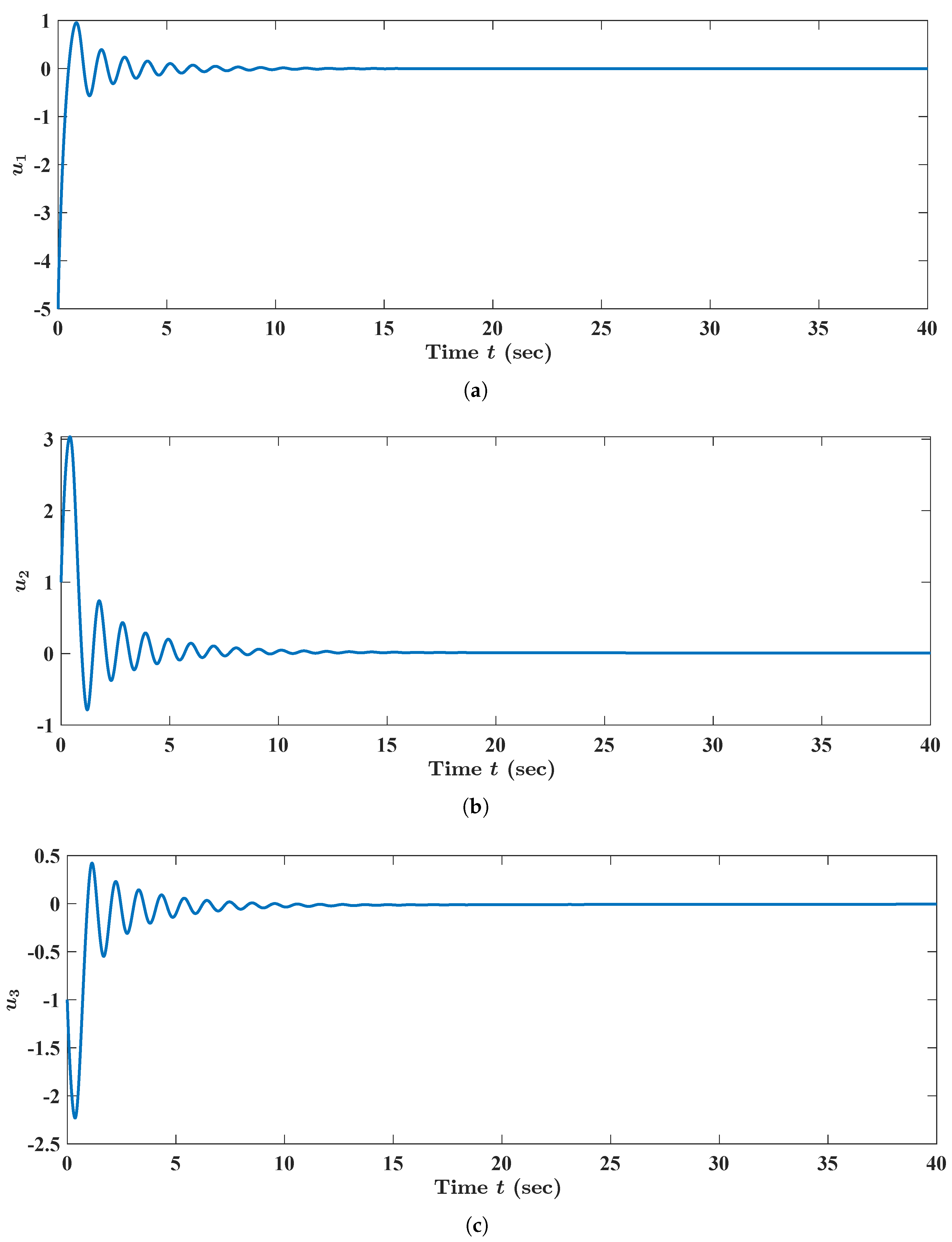
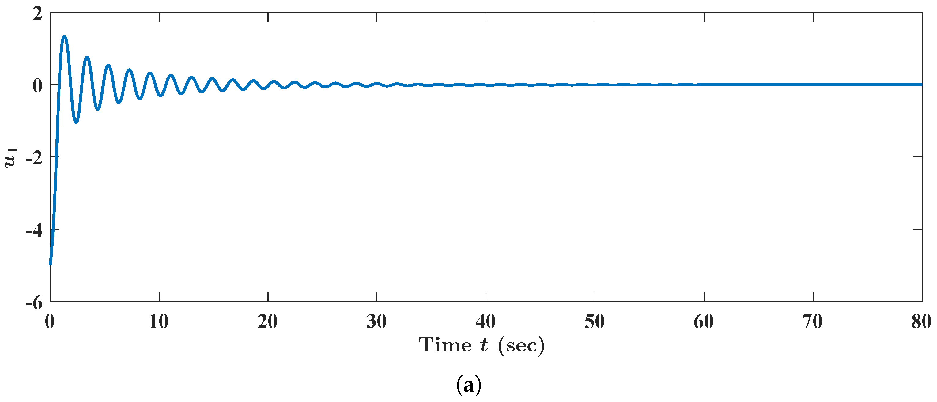
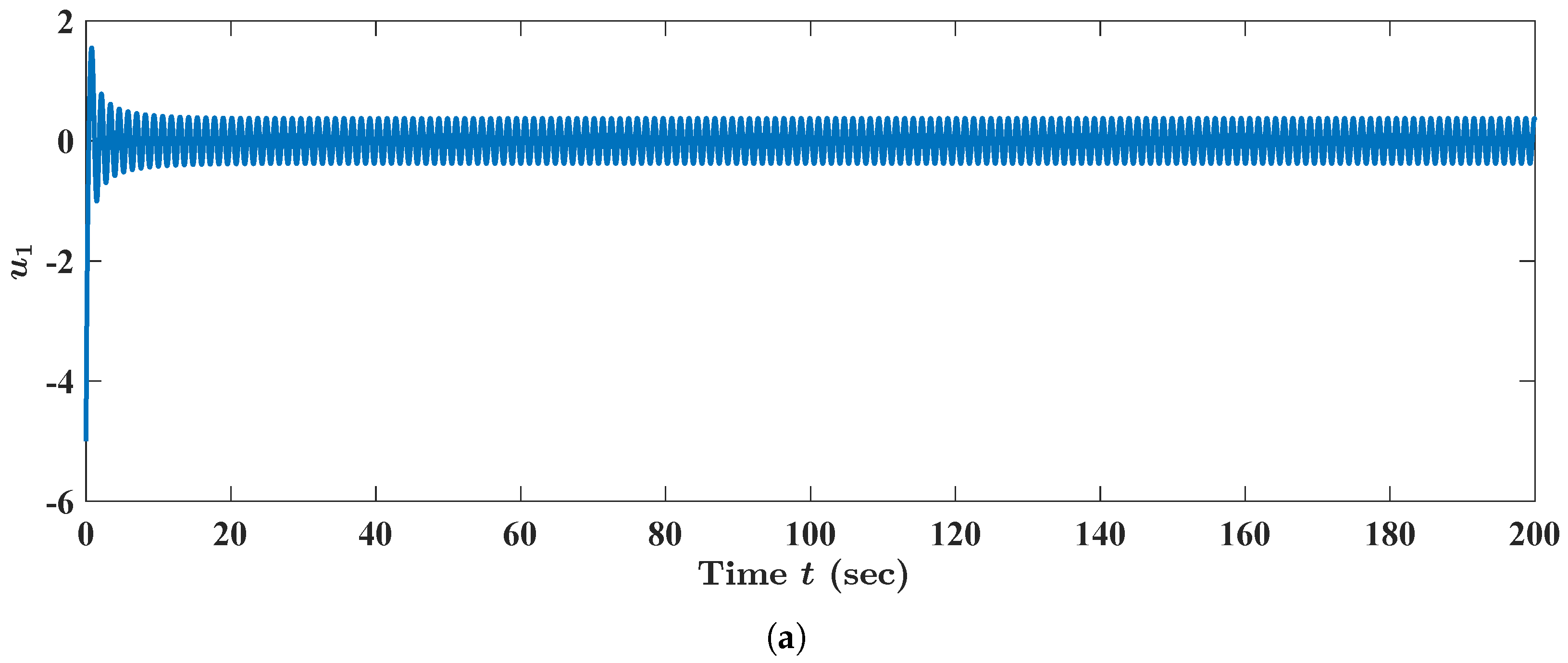
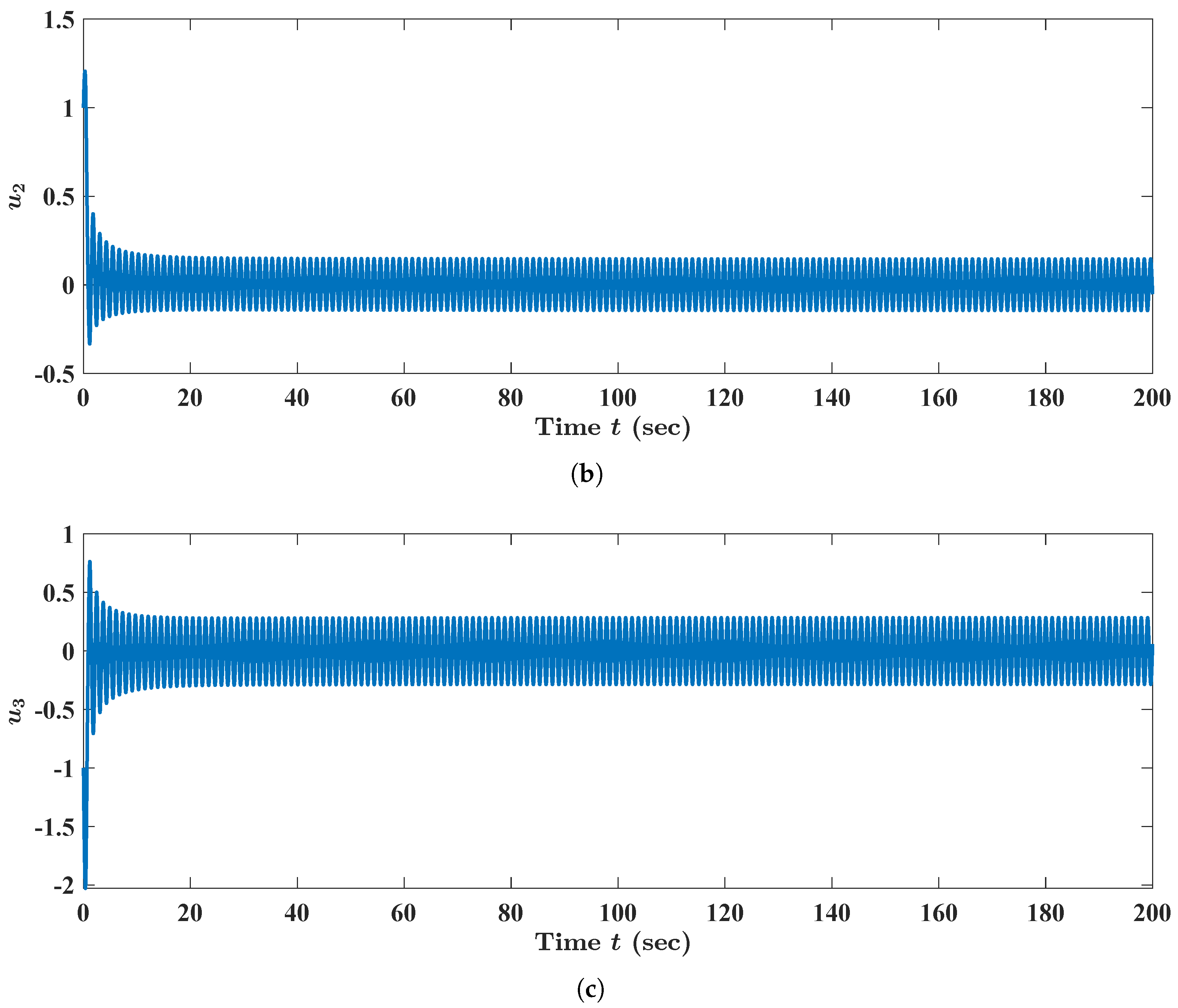
We visualize here the aforementioned Hopf bifurcation phenomenon in FBAMNN (
118) with
. For this purpose, based on MATLAB, we fixed
, as well as
, to numerically compute the state trajectory
of FBAMNN (
118), which is supplemented by the initial condition
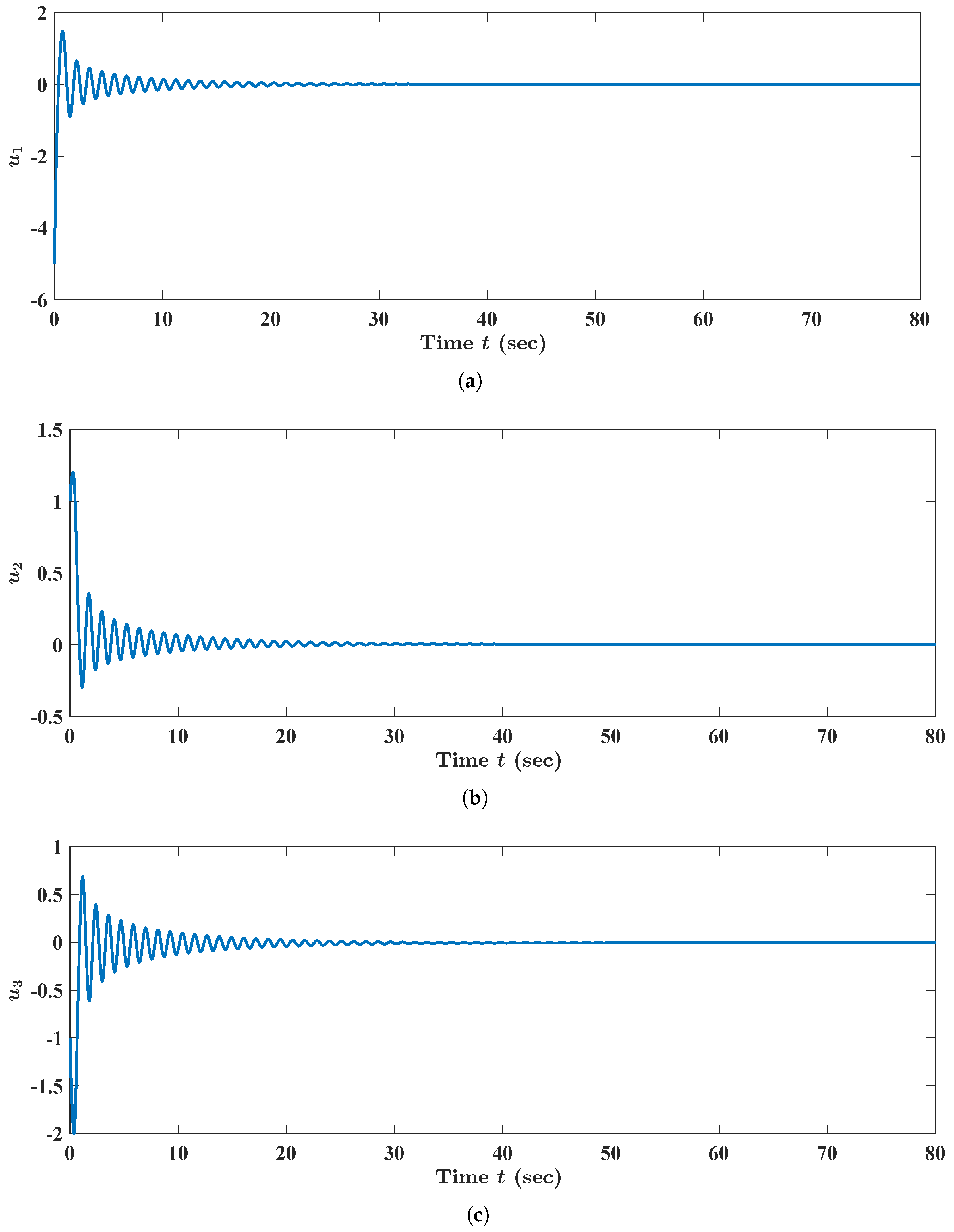
By scrutinizing
Figure 1, we can conclude that the state trajectory
of FBAMNN (
118), with
and
, tends to the null state trajectory
as time
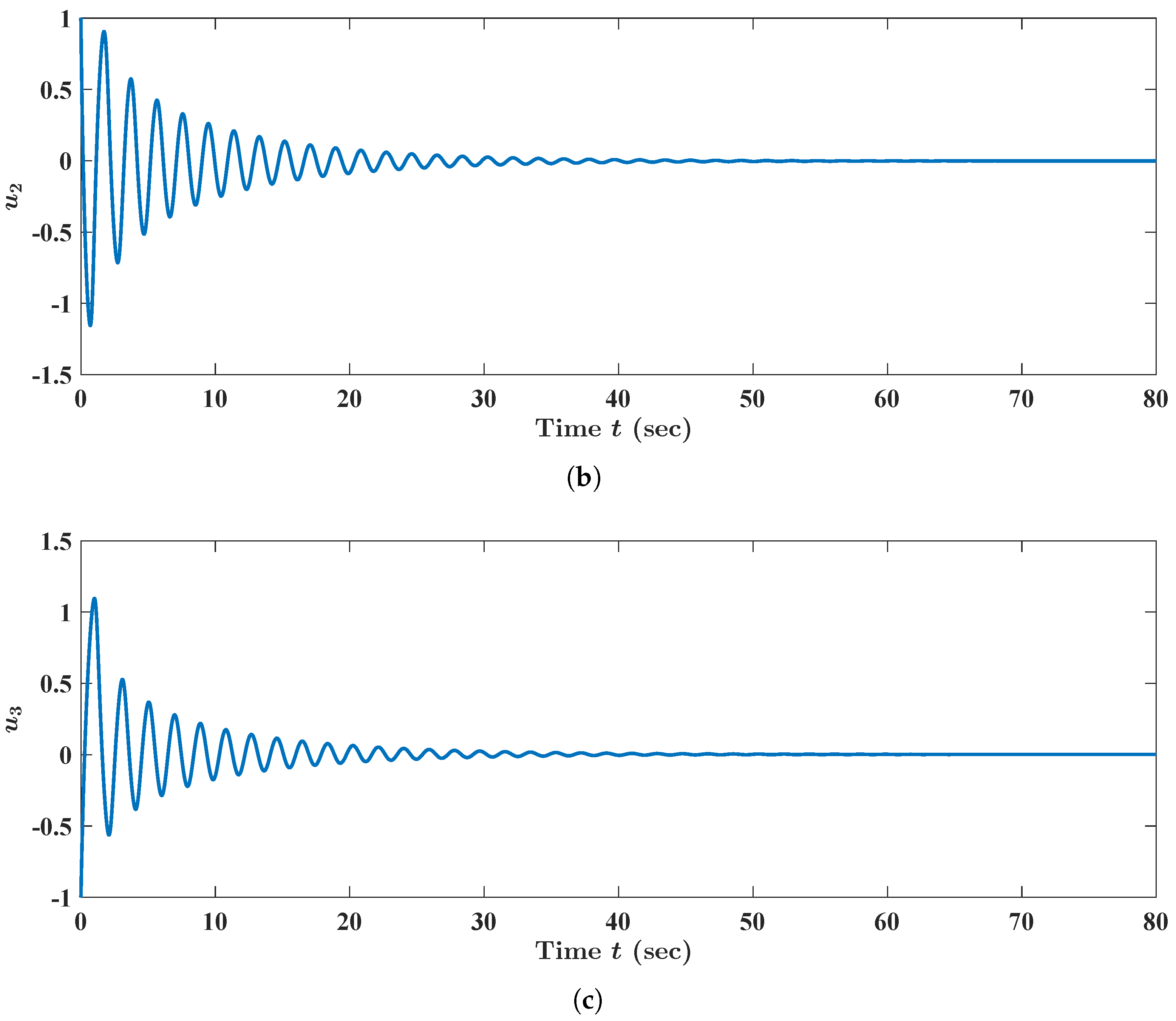
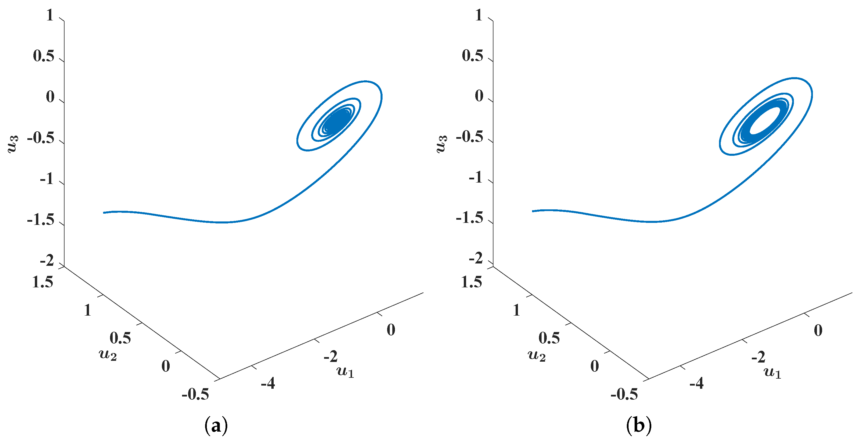
t escapes to infinity. We plotted, via MATLAB, the state trajectory
of FBAMNN (
118), with
and
in the phase space to obtain
Figure 2a; we also found that the state trajectory
approached the equilibrium state
in the phase space as time
t tended to infinity. On the other hand, we fixed
, as well as
, which we numerically computed, based on MATLAB, the state trajectory
of FBAMNN (
118), which was supplemented by the initial Condition (
120). Through viewing
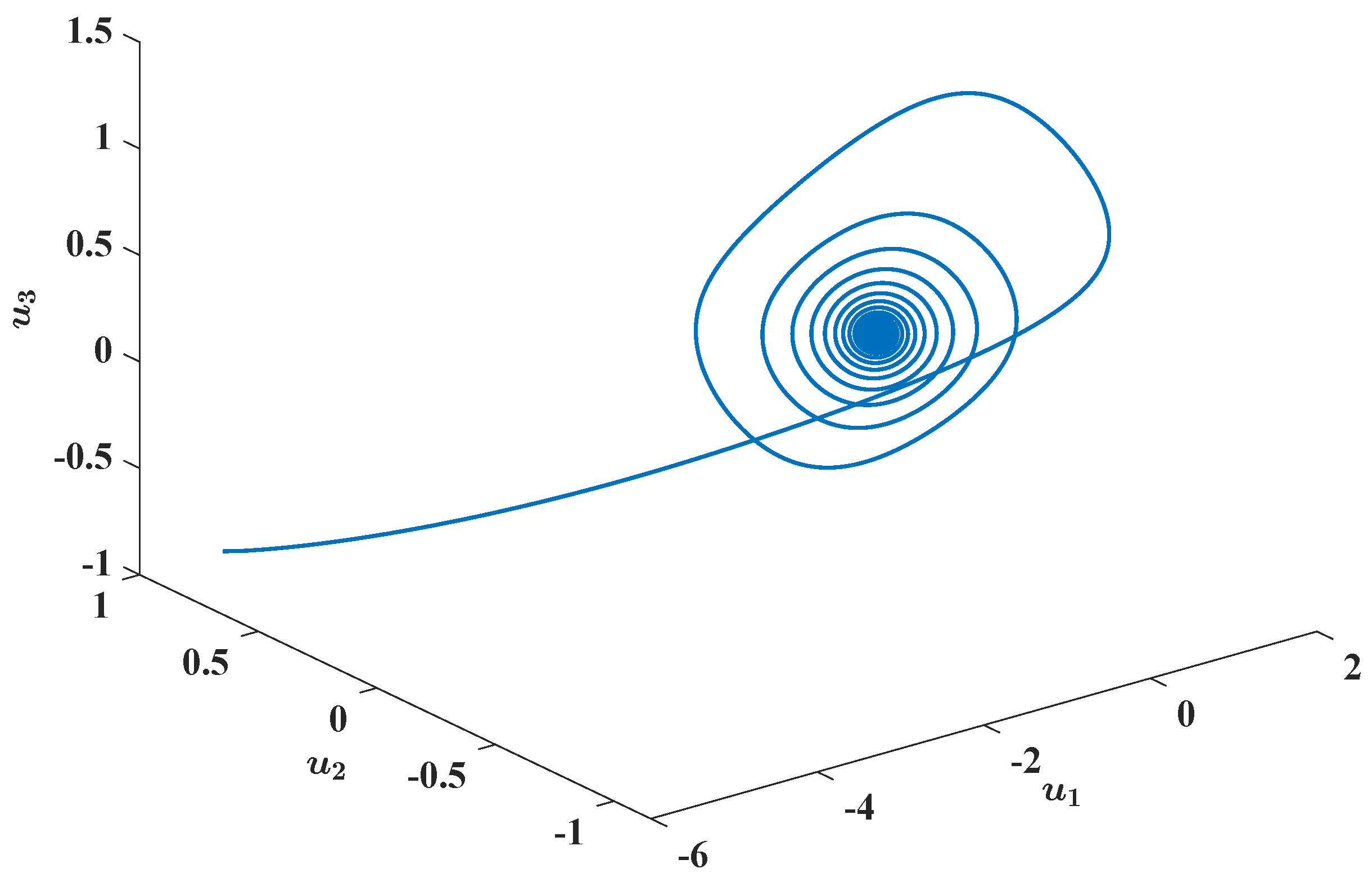
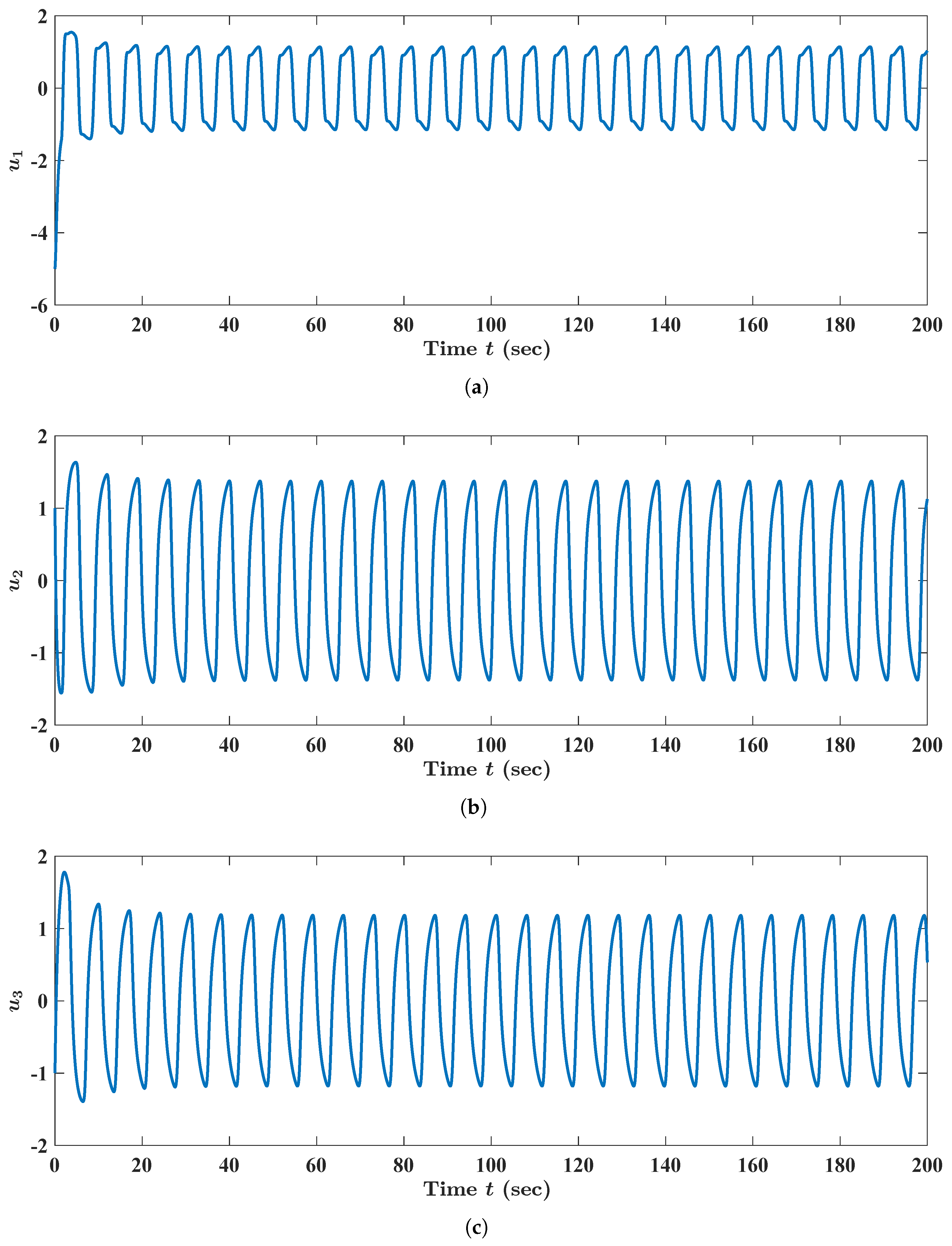
Figure 3, we concluded that the state trajectory
of FBAMNN (
118), with
and
, tended to a periodic state trajectory as time
t approached infinity. We plotted, via MATLAB, the state trajectory
of FBAMNN (
118), with
and
in the phase space to obtain
Figure 2b; in addition, we found that the state trajectory
approached a non-trivial closed curve in the phase space as time
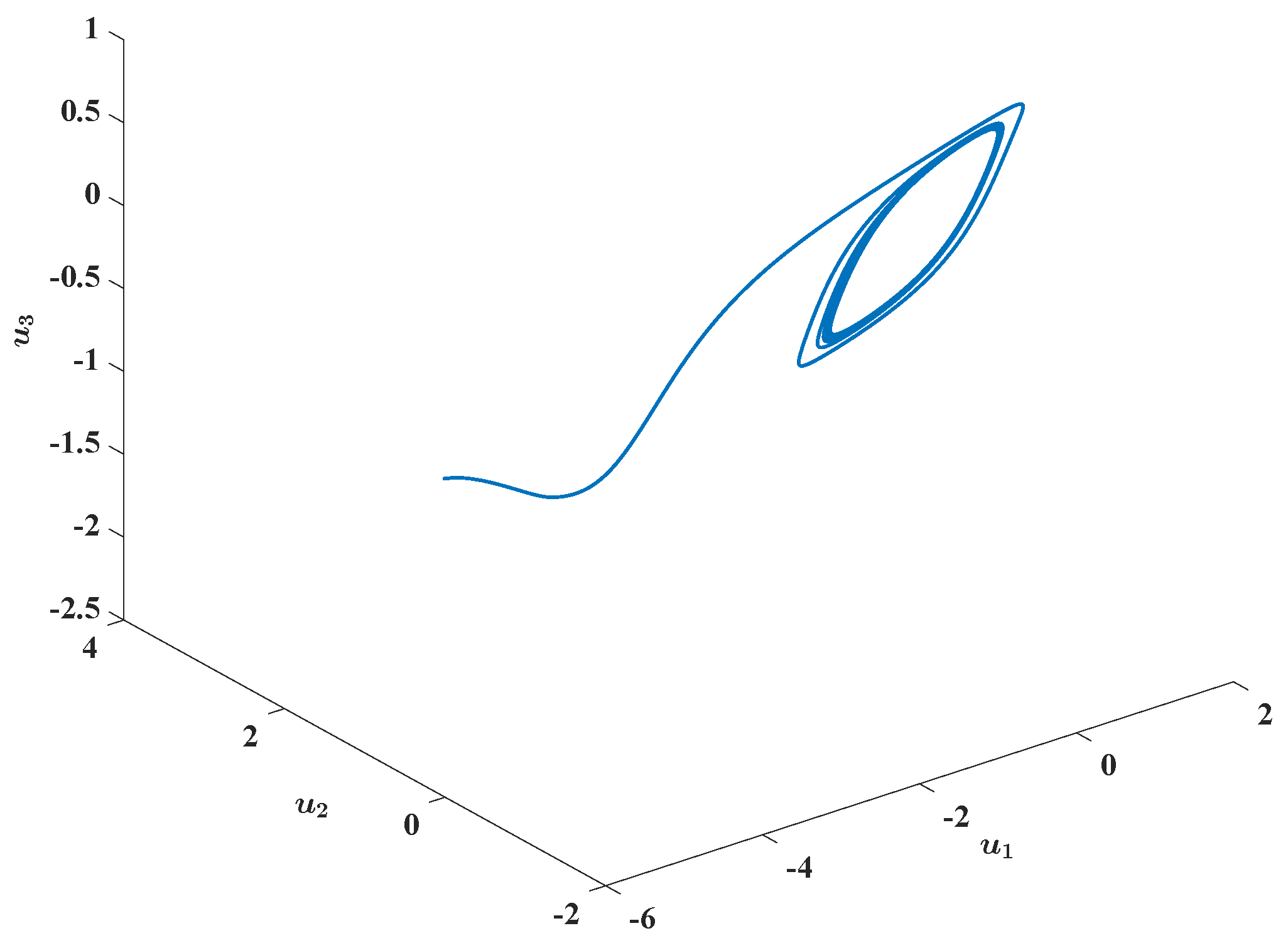
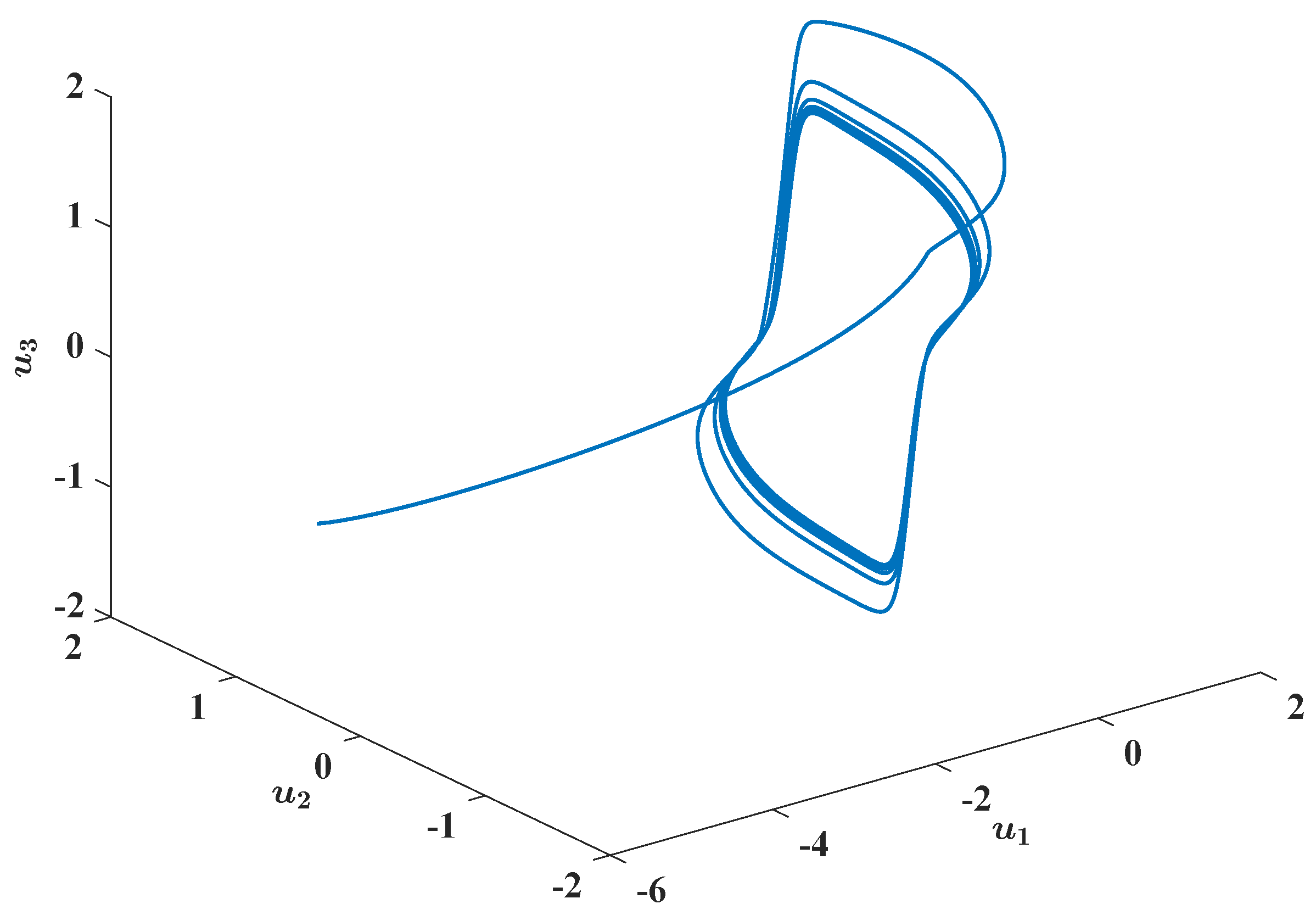
t went to infinity. To display more clearly the existence of the periodic state trajectory in FBAMNN (
118), with
, we plotted—based on MATLAB—the state trajectory
of FBAMNN (
118), with
and
, in the phase space to obtain
Figure 4; in this figure, we can see more clearly the existence of the periodic state trajectory in FBAMNN (
118) with
). In
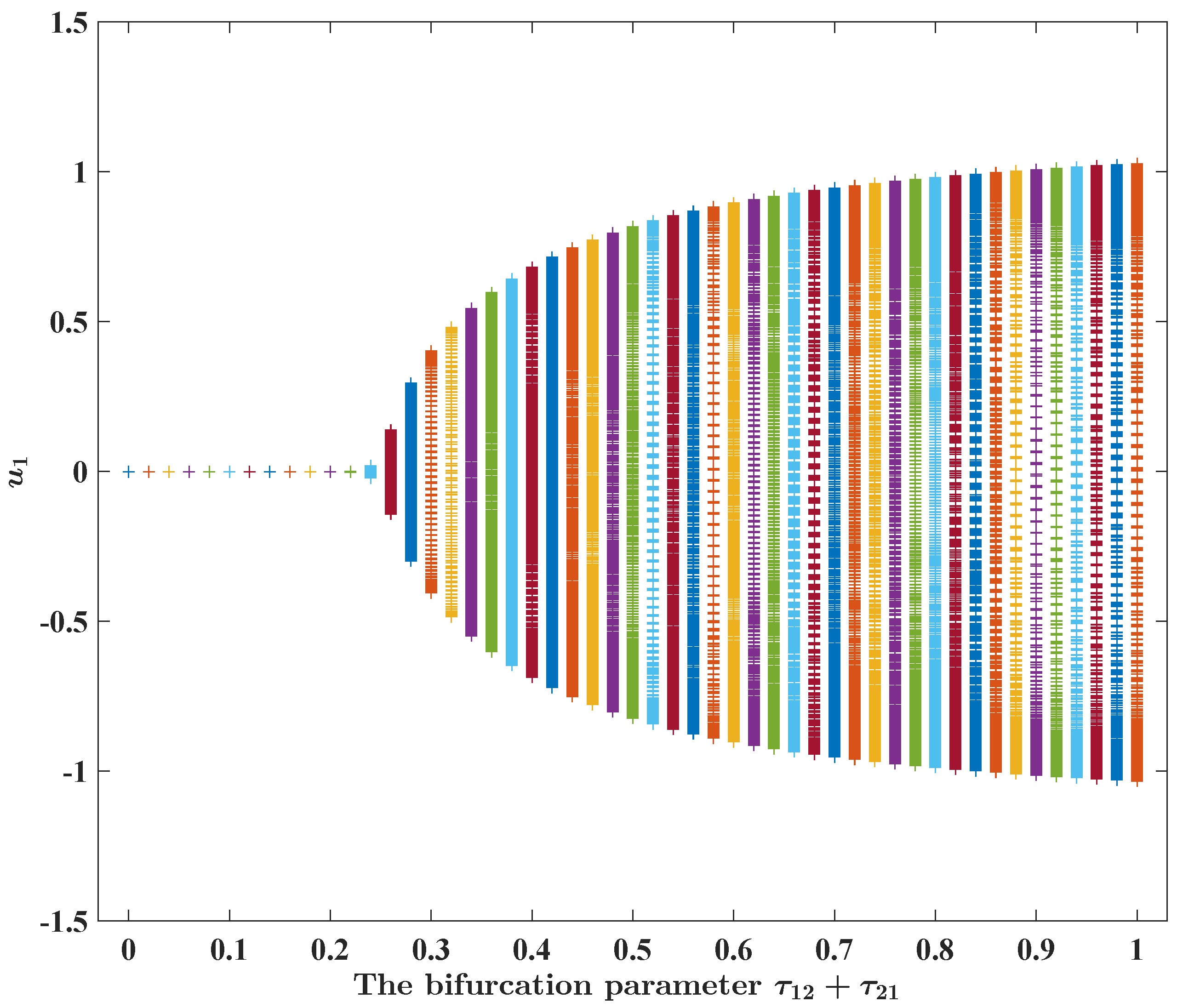
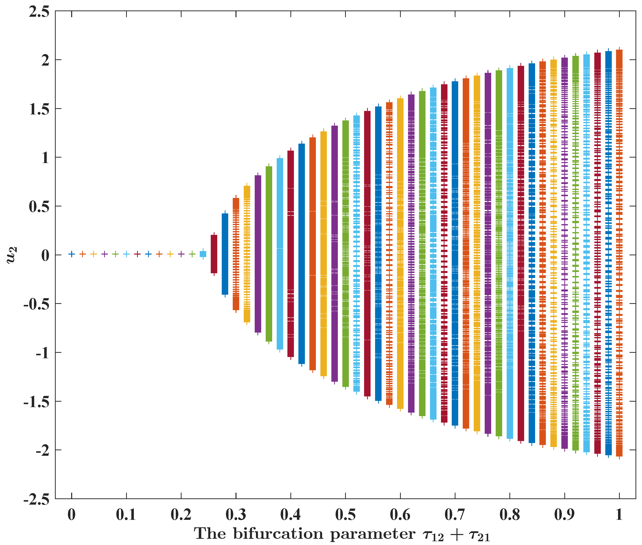
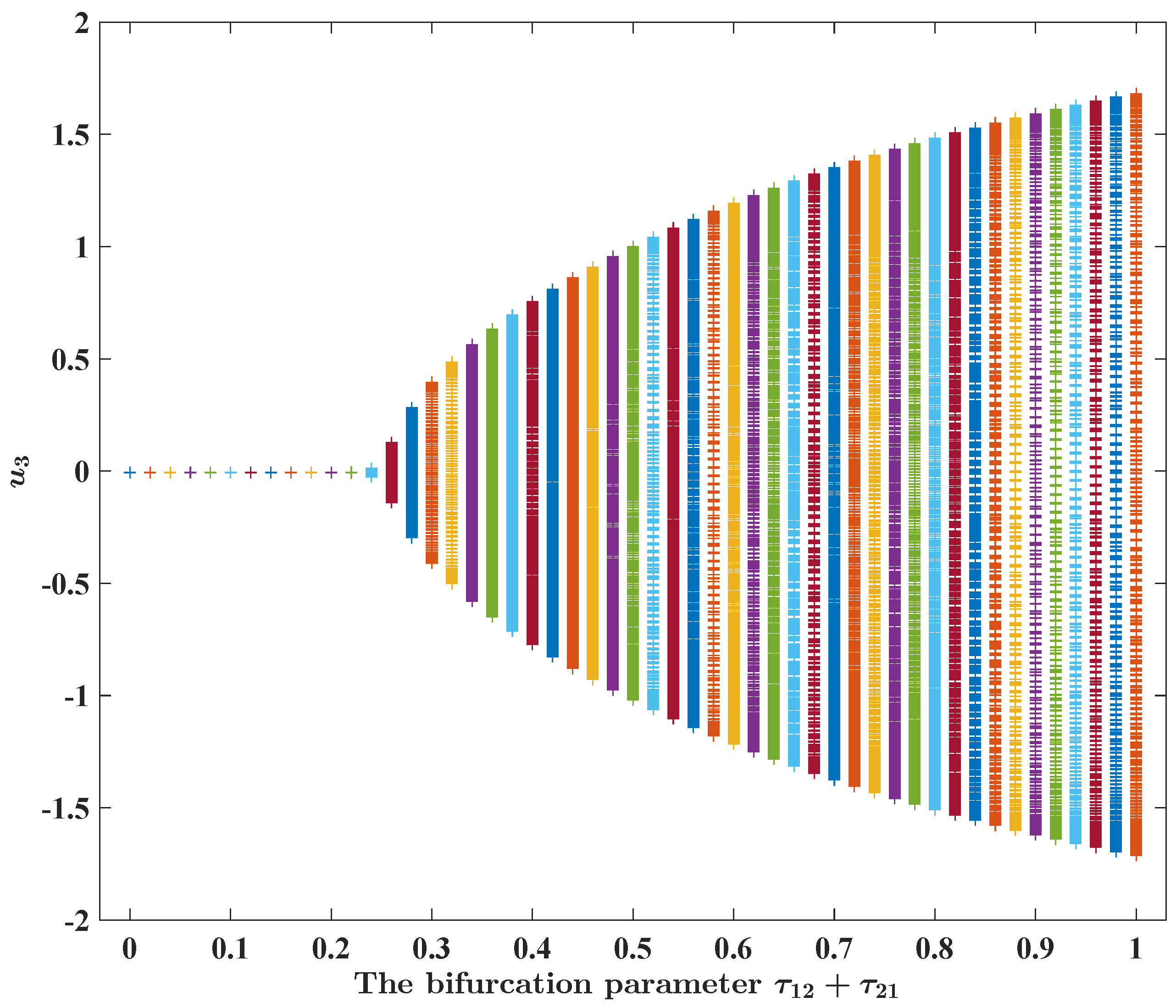
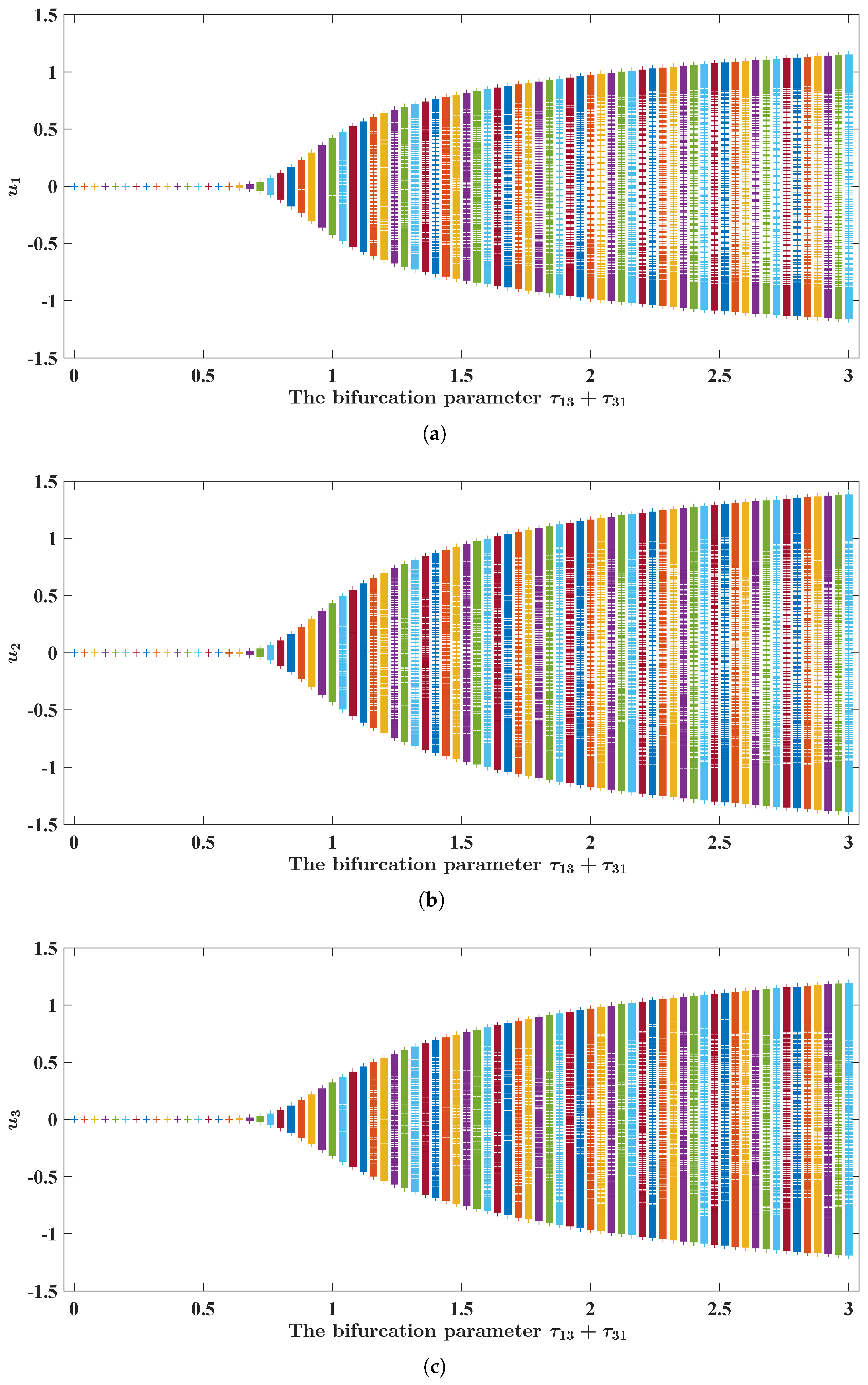
Figure 5,
Figure 6 and
Figure 7, we found that a Hopf bifurcation occurred at the point
in the FBAMNN detailed in Example 1 (that is, FBAMNN (
118) with
).
Example 2. Let , as well as the constants and that were given in the closed half interval . We perform here some bifurcation analyses of the following FBAMNN It is evident that
is an equilibrium state of FBAMNN (
121). As with FBAMNN (
118), we linearized FBAMNN (
121) at the equilibrium state
to obtain
where the time delay
and
satisfy
.
Figure 1.
Numerical and graphical illustrations of the stability of equilibrium states of FBAMNN (
4) with
and with
, which are viewed as the bifurcation parameter and are strictly less than a threshold constant. In addition,
is the (unique) state trajectory triplet of FBAMNN (
118), with
(in actuality,
), which is strictly less than the threshold constant (namely the bifurcation point)
. This is approximately equal to
, with
, such that the initial Condition (
120) is satisfied. Equivalently, it could such that it holds that
is for all
,
, as well as for all
and
. The graph (curve) of the function
, which is the first component of the aforementioned state trajectory triplet
,
, is plotted in (
a). The graph (curve) of the function
, which is the second component of the aforementioned state trajectory triplet
,
, is plotted in (
b). The graph (curve) of the function
, which is the third component of the aforementioned state trajectory triplet
,
, is plotted in (
c).
![Fractalfract 08 00083 g001]()
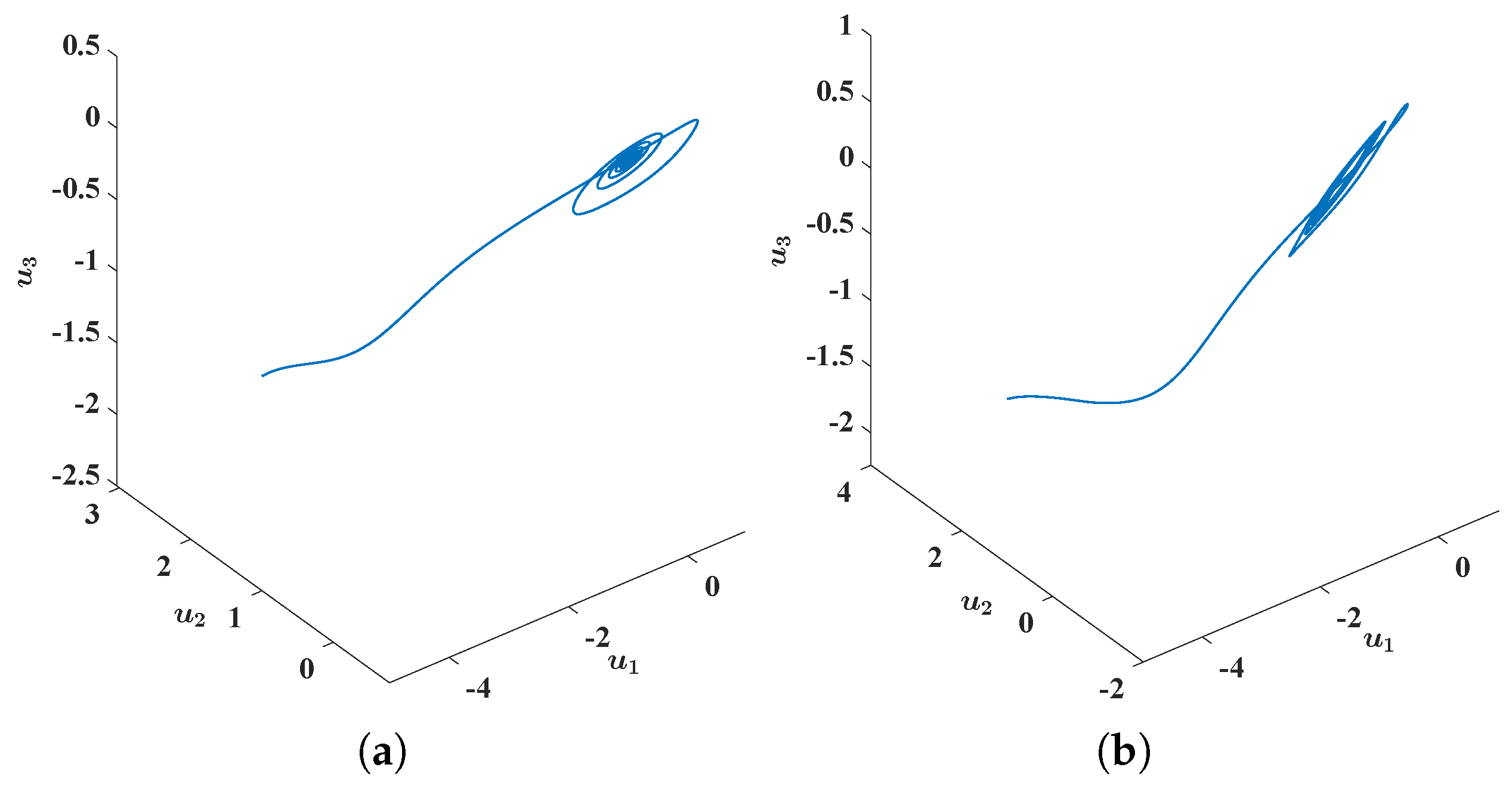
Figure 2.
Numerical and graphical illustrations of FBAMNN (
4) with
, which undergoes Hopf bifurcation at
. In (
a), it is plotted that the graph (a parameterized space curve) of the (unique) state trajectory triplet
of FBAMNN (
118), with
(in actuality,
), is strictly less than the threshold constant (namely the bifurcation point)
, which is approximately equal to
and
, such that the initial Condition (
120) is satisfied. Equivalently, it could be such that it holds that
is for all
, and that
is for all
and
. In (
b), it is plotted that the graph (a parameterized space curve) of the (unique) state trajectory triplet
of FBAMNN (
118), with
(in actuality,
), is strictly greater than the threshold constant (namely the bifurcation point)
, which is approximately equal to
and
, such that the initial condition (
120) is satisfied. Equivalently, it could such that it holds that
is for all
, and that
is for all
and
.
![Fractalfract 08 00083 g002]()
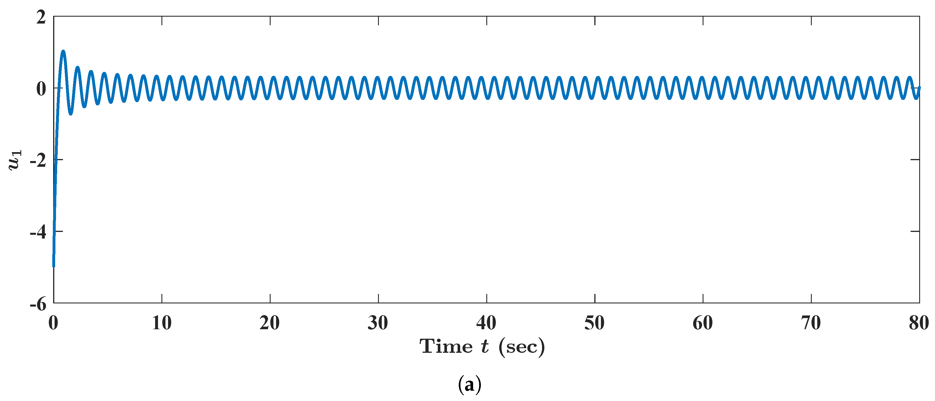
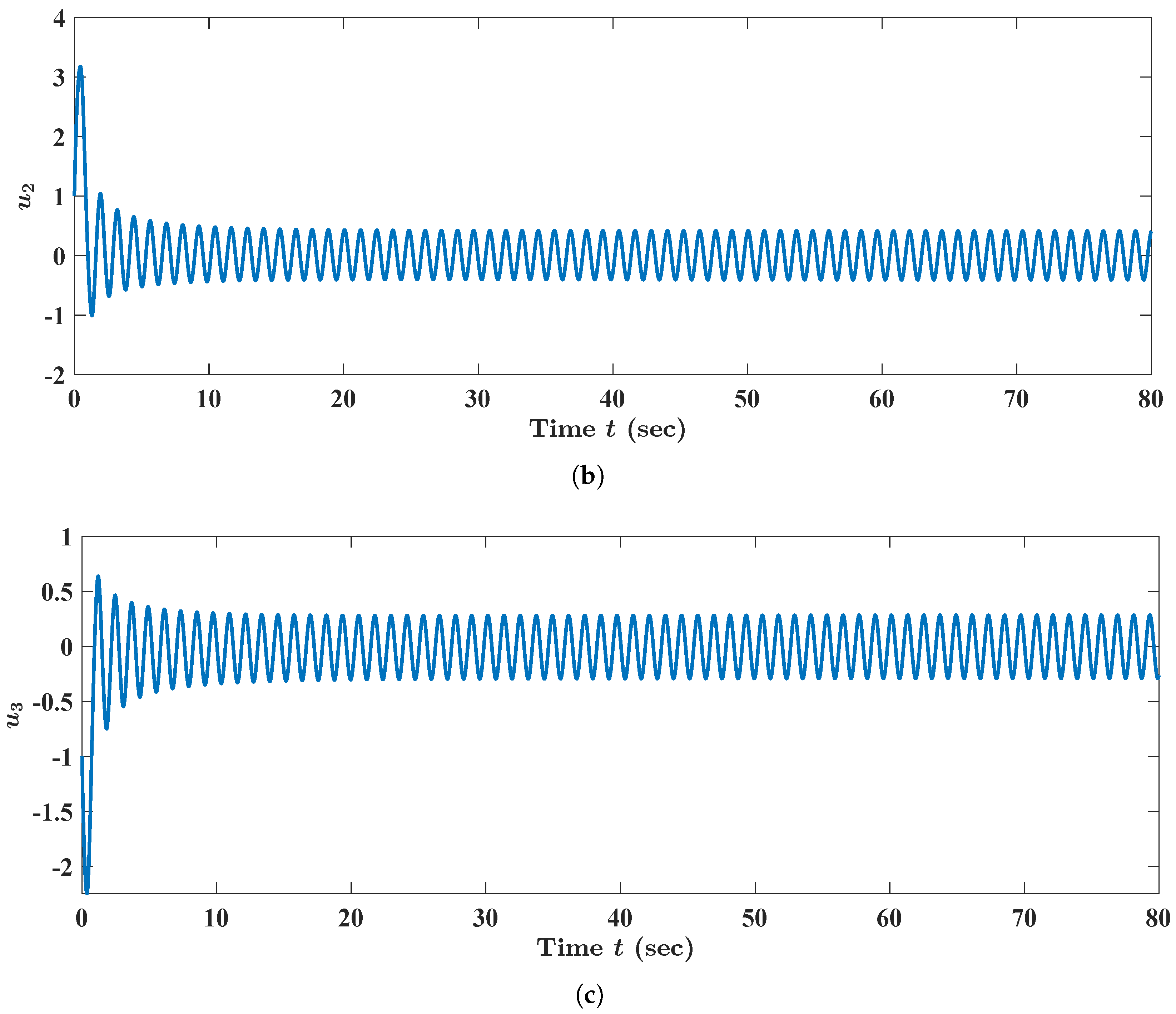
Figure 3.
Numerical and graphical illustrations of the existence and the (asymptotical) stability of the periodic state trajectories of FBAMNN (
4) with
and with
, where the bifurcation parameter is strictly greater than a threshold constant and is opposed to
Figure 1. As with
Figure 1,
is the (unique) state trajectory triplet of FBAMNN (
118), with
(in actuality,
), which is strictly greater than the threshold constant (namely the bifurcation point)
. This is approximately equal to
and
, such that the initial Condition (
120) is satisfied. Equivalently, it could be such that it holds that
for all
, and that
is for all
and
. The graph (curve) of the function
, which is the first component of the aforementioned state trajectory triplet
,
, is plotted in (
a). The graph (curve) of the function
, which is the second component of the aforementioned state trajectory triplet
,
, is plotted in (
b). The graph (curve) of the function
, which is the third component of the aforementioned state trajectory triplet
,
, is plotted in (
c).
![Fractalfract 08 00083 g003a]()
![Fractalfract 08 00083 g003b]()
Figure 4.
Numerical and graphical illustration of the existence and the (asymptotical) stability of periodic state trajectories of FBAMNN (
4), with
and
, where the bifurcation parameter is strictly greater than a threshold constant. In
Figure 4, it is plotted in the phase space that the graph (which shows a parameterized space curve) of the (unique) state trajectory triplet
of FBAMNN (
118), with
(in actuality,
), is strictly greater than the threshold constant (namely the bifurcation point)
, which is approximately equal to
and
, such that the initial condition (
120) is satisfied. Equivalently, it could be such that it holds that
is for all
, and that
is for all
and
.
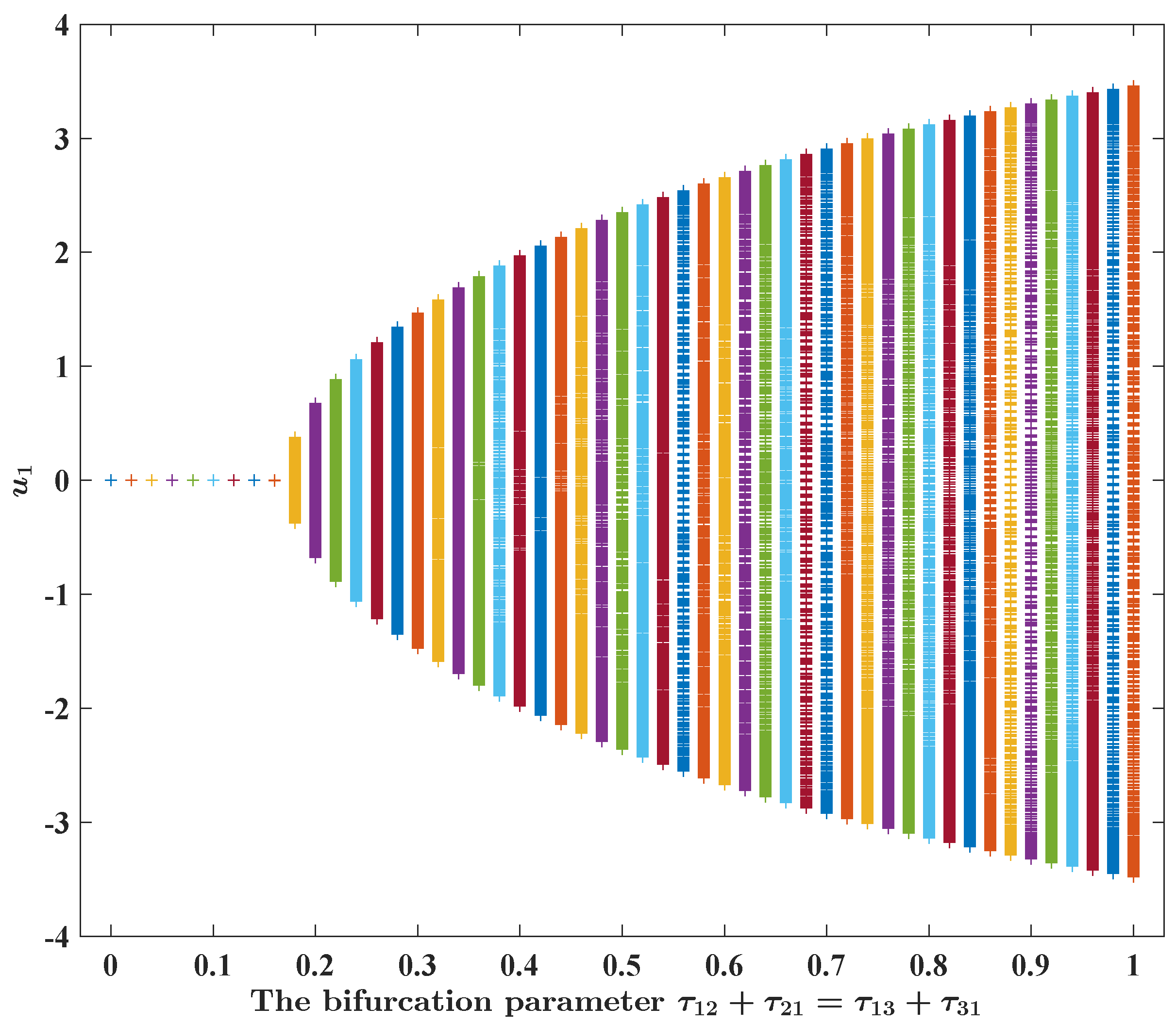
Figure 5.
Numerical and graphical illustration of FBAMNN (
4), with
, which undergoes Hopf bifurcation at
. In
Figure 5, it is plotted that the bifurcation diagram of FBAMNN (
118), with
and
, is the bifurcation parameter in terms of the
component.
Figure 5.
Numerical and graphical illustration of FBAMNN (
4), with
, which undergoes Hopf bifurcation at
. In
Figure 5, it is plotted that the bifurcation diagram of FBAMNN (
118), with
and
, is the bifurcation parameter in terms of the
component.
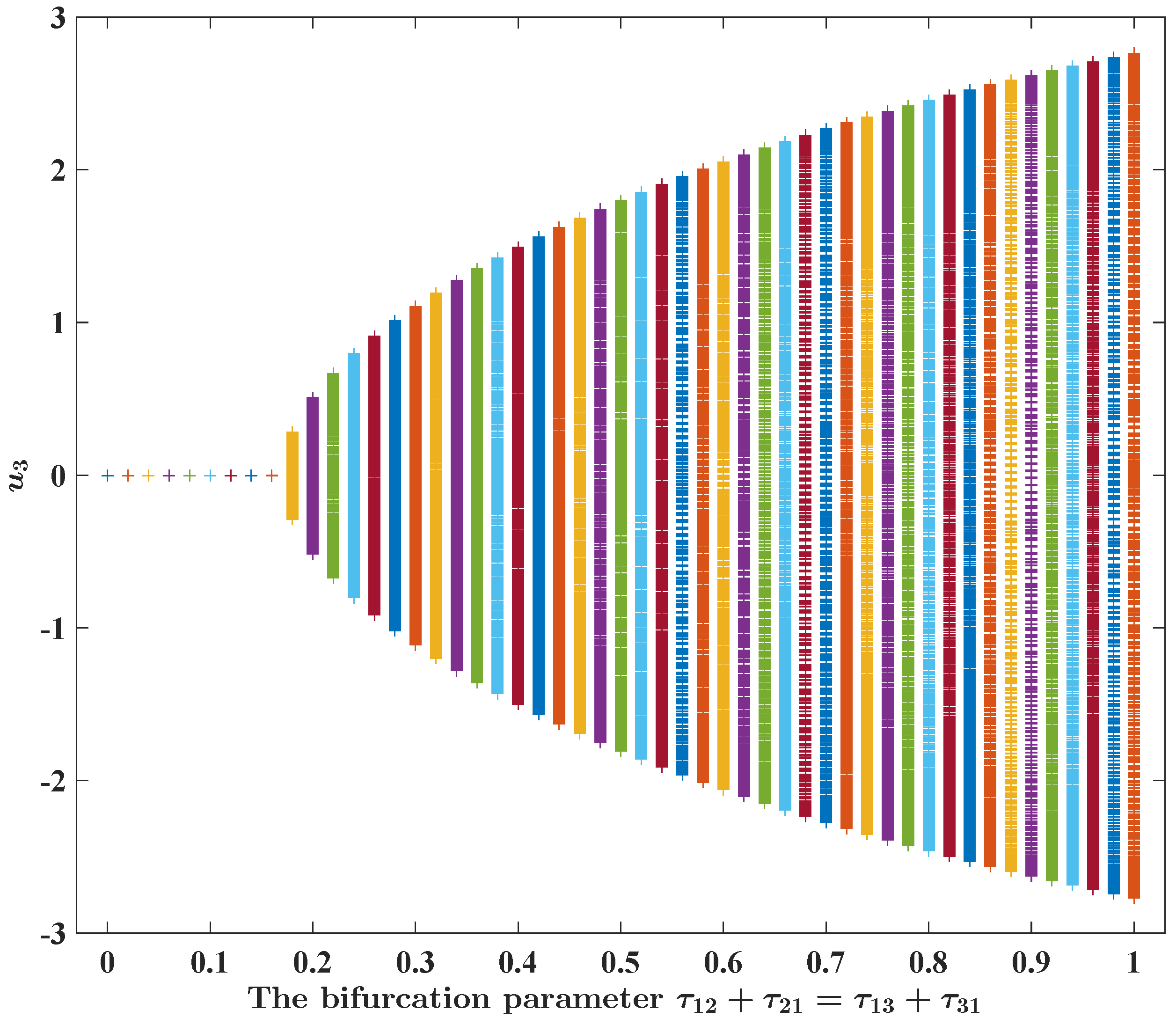
Figure 6.
Numerical and graphical illustration of FBAMNN (
4), with
, which undergoes Hopf bifurcation at
. In
Figure 6, it is plotted that the bifurcation diagram of FBAMNN (
118), with
and
, is the bifurcation parameter in terms of the
component.
Figure 6.
Numerical and graphical illustration of FBAMNN (
4), with
, which undergoes Hopf bifurcation at
. In
Figure 6, it is plotted that the bifurcation diagram of FBAMNN (
118), with
and
, is the bifurcation parameter in terms of the
component.
Figure 7.
Numerical and graphical illustration of FBAMNN (
4), with
, which undergoes Hopf bifurcation at
. In
Figure 7, it is plotted that the bifurcation diagram of FBAMNN (
118), with
and
, is the bifurcation parameter in terms of the
component.
Figure 7.
Numerical and graphical illustration of FBAMNN (
4), with
, which undergoes Hopf bifurcation at
. In
Figure 7, it is plotted that the bifurcation diagram of FBAMNN (
118), with
and
, is the bifurcation parameter in terms of the
component.
We analyzed FBAMNN (
121) (with
), as well as the linearized FBAMNN (
122) (with
), to conclude that there exists a positive constant
(which is approximately equal to
and was numerically calculated via MATLAB) such that the following applies: If
and
, then the equilibrium state
of FBAMNN (
121) is (at least locally) asymptotically stable; if
, FBAMNN (
121), is involved with the parameters
and
, it undergoes Hopf bifurcation at point
.
We visualize here the aforementioned Hopf bifurcation phenomenon in FBAMNN (
121) (with
). For this purpose, we fixed
, as well as
, and we numerically computed, based on MATLAB, the state trajectory
of FBAMNN (
121), which was supplemented by the initial condition
By carefully examining
Figure 8, we concluded that the state trajectory
of FBAMNN (
121) (with
and
) tended to the null state trajectory
as time
t escaped to infinity. We plotted, via MATLAB, the state trajectory
of FBAMNN (
121) (with
and
) in the phase space to obtain
Figure 9; we found that the state trajectory
approached the equilibrium state
in the phase space as time
t tended to infinity. On the other hand, we fixed
, as well as
, and numerically computed, based on MATLAB, the state trajectory
of FBAMNN (
121), which was supplemented by the initial Condition (
123). By viewing
Figure 10, we concluded that the state trajectory
(with
and
) tended to a periodic state trajectory as time
t approached infinity. We plotted, via MATLAB, the state trajectory
of FBAMNN (
121) (with
and
) in the phase space to obtain
Figure 11; we found that the state trajectory
approached a non-trivial closed curve in the phase space as time
t went to infinity. In
Figure 12, we found that a Hopf bifurcation occurred at point
in the FBAMNN in Example 2 (that is, FBAMNN (
121) with
).
Example 3. Let the constants , , , and be given in the closed half interval , such that . We perform here some bifurcation analyses of the following FBAMNN equation: It is evident that
is an equilibrium state of FBAMNN (
124). As with FBAMNNs (
118) and (
121), we linearized FBAMNN (
124) at the equilibrium state
to obtain
in which the time delay
,
,
, and
satisfy
.
We analyzed FBAMNN (
124), as well as the linearized FBAMNN (
125), to conclude that there exists a positive constant
(which is approximately equal to
and was numerically calculated via MATLAB), such that the following applies: If
, then the equilibrium state
of FBAMNN (
124) is (at least locally) asymptotically stable; moreover, FBAMNN (
124) undergoes Hopf bifurcation at point
.
We visualize here the aforementioned Hopf bifurcation phenomenon in FBAMNN (
124) (with
). For this purpose, we fixed
, as well as numerically computed, based on MATLAB, the state trajectory
of FBAMNN (
124), which was supplemented by the initial condition
By viewing
Figure 13, we concluded that the state trajectory
of FBAMNN (
124) (
) tended to the null state trajectory
as time
t escaped to infinity. We plotted, via MATLAB, the state trajectory
of FBAMNN (
124) (with
) in the phase space to obtain
Figure 14a; we found that the state trajectory
approached the equilibrium state
in the phase space as time
t tended to infinity. On the other hand, we fixed
and numerically computed, based on MATLAB, the state trajectory
of FBAMNN (
124), which was supplemented by the initial condition (
126). By viewing
Figure 15, we concluded that the state trajectory
of FBAMNN (
124) (with
) tended to a periodic state trajectory as time
t approached infinity. We plotted, via MATLAB, the state trajectory
of FBAMNN (
118) (with
) in the phase space to obtain
Figure 14b; we found that the state trajectory
approached a non-trivial closed curve in the phase space as time
t went to infinity. In
Figure 16,
Figure 17 and
Figure 18, we found that a Hopf bifurcation occurred at the point
in the FBAMNN equation in Example 3 (that is, FBAMNN (
124) with
).


