Analysis of a Fractional-Order Model for African Swine Fever with Effect of Limited Medical Resources

Abstract

In this paper, a fractional-order model for African swine fever with limited medical resources is proposed and analyzed. First, the existence and uniqueness of a positive solution is proven. Second, the basic reproduction number and the conditions sufficient for the existence of two equilibriums are obtained. Third, the local stability of the two equilibriums is studied. Next, some numerical simulations are performed to verify the theoretical results. The mathematical and simulation results show that the values of some parameters, such as fractional order and medical resources, are critical for the stability of the equilibriums.

1. Introduction

African swine fever (ASF) is a highly contagious disease with a high fatality rate, and which poses a great threat to the pig industry. The main symptoms of the disease in pigs include high fever, aphagia, and extensive skin and visceral bleeding. African swine fever virus (ASFV) has been spreading in Africa, Asia, Europe, and other regions for more than one hundred years, since it was discovered in Kenya in 1921, and it has caused immeasurable losses to the global pig industry [1]. Since African swine fever was discovered in Shenyang City in August of 2018, more than one hundred cases of ASF had occurred in 28 provinces of China by February, 2019, and the number of pigs culled was up to one million [2]. Due to the absence of effective vaccines, the available method to control this disease is to isolate and slaughter infected animals in affected areas, which inevitably results in high economic losses.

In recent years, mathematical models have played an important role in analyzing the spread and control of all kinds of infectious diseases [3,4,5,6]. Since the outbreak of African swine fever, researchers have established many models to analyze its spread. Pietschmann et al. reviewed the main characteristics, clinical features, and transmission modes of pathogenic viruses [7]. The results showed that very low doses of ASFV infected other animals through the mouth, nose, and direct contact. Guinat et al. used a stochastic SEIR model to study the transmission of ASFV and estimated the basic reproduction number $R_0$ of the Georgia 2007/1 strain through parameters estimated from transmission experiments [8]. Their results suggested that detection of ASFV genomes in nose and mouth specimens is an effective diagnostic tool for early detection of infection. Mur et al. used a spatially explicit stochastic transmission model to understand the dynamics of ASFV infection among domestic pig farms [9]. The results showed that indirect transmission through pathogens between farms within a 2 km radius is the most common mode of transmission. Barongo et al. established a stochastic model to simulate the transmission dynamics of ASFV under different interventions [10]. The results confirmed the importance of early intervention and implementation of biosafety measures. Recently, the control of African swine fever virus in large-scale pig farms was considered in [11], and the dynamics of African swine fever with culling in China were analyzed in [12].

In recent decades, fractional-order calculus has been widely studied and applied in many fields, such as physics [13,14], chemistry [15], biology [16,17], epidemiology [18,19,20], and other fields [21,22,23,24,25,26,27]. Fractional-order models can reflect the complex behaviors of various diseases more accurately and deeply than classical integer-order models. Fractional-order systems are better than integer-order systems because they contain the genetic characteristics of memory [28]. There are different definitions of fractional calculus, such as Riemann–Liouville (RL), Caputo, Grunwald–Letnikov (GL), etc. These definitions all have advantages and disadvantages, and in this paper will use the Caputo definition to carry out research, because the fractional-order equations under the Caputo definition have the the same initial condition as the integer order. As the initial value of the fractional derivative is difficult to find and has no clear physical meaning, the advantages of the Caputo definition make its application more popular.

In the real world, medical resources are always limited (such as drugs, isolation locations, etc.), so it is necessary to select an appropriate treatment function when constructing a model. In [29], Cui et al. introduced the saturation function to the model to describe the situation of limited medical resources. Inspired by [11,12,28,29,30], we established the following model

$$\left\{\begin{array}{ccc}{D}^{\alpha }S\left(t\right)\hfill & =\hfill & \mathrm{\Lambda }-\beta S\left(t\right)I\left(t\right)-\mu S\left(t\right)+\delta R\left(t\right),\hfill \\ D^{\alpha }E\left(t\right)\hfill & =\hfill & \beta S\left(t\right)I\left(t\right)-(\omega +\mu )E\left(t\right),\hfill \\ D^{\alpha }I\left(t\right)\hfill & =\hfill & {\displaystyle \omega E\left(t\right)-(\mu +d)I\left(t\right)-\frac{cI\left(t\right)}{b+I\left(t\right)},}\hfill \\ D^{\alpha }Q\left(t\right)\hfill & =\hfill & {\displaystyle \frac{cI\left(t\right)}{b+I\left(t\right)}-(ϵ+\mu )Q\left(t\right),}\hfill \\ D^{\alpha }R\left(t\right)\hfill & =\hfill & ϵQ\left(t\right)-(\mu +\delta )R\left(t\right),\hfill \end{array}\right.$$

(1)

where $D^{\alpha }$ is the Caputo fractional derivative of order $\alpha$, with $0<\alpha \le 1$. The descriptions of variables and parameters in system (1) are listed in Table 1, and all parameters are assumed to be positive. Here, we use the saturation function $\frac{cI}{b+I}$ to depict the limited medical resources.

Table 1. Description of variables and parameters in system (1).

Variables	Descriptions
$S\left(t\right)$	Density of the susceptible population
$E\left(t\right)$	Density of the exposed population
$I\left(t\right)$	Density of the infection population
$Q\left(t\right)$	Density of the quarantined population
$R\left(t\right)$	Density of the recovered population
Parameters	Descriptions	Values
$\mathrm{\Lambda }$	The constant recruitment rates of population	[1, 1.75]
$\beta$	Effective contact rate between the susceptible and the infection population	[0.001, 0.3]
$\omega$	The average rate at which an individual passes through the incubation period	[0.12, 0.35]
$ϵ$	Recovery rate of the quarantined	[0.01, 0.8]
$\delta$	The constant rate at which the recovered population become susceptible	[0.01, 0.3]
d	Death rate due to the disease	[0.002, 0.0035]
$\mu$	Natural death rate	[0.08, 0.25]
c	The maximum isolation rate per unit of time	[1, 10]
b	The infection scale	[1, 5]

We denote $N\left(t\right)$ as the total population, then $N\left(t\right)=S\left(t\right)+E\left(t\right)+I\left(t\right)+Q\left(t\right)+R\left(t\right)$. From system (1), we can obtain the following differential inequality:

$$D^{\alpha }N\left(t\right)=\mathrm{\Lambda }-\mu N\left(t\right)-dI\left(t\right)\le \mathrm{\Lambda }-\mu N\left(t\right),$$

and from the above, we can further obtain ${\displaystyle N\left(t\right)\le \frac{\mathrm{\Lambda }}{\mu }}$, as $t\to +\infty$. Denote the biologically feasible region for system (1) as $\mathrm{\Gamma }$, then it will be

$$\mathrm{\Gamma }=\left\{(S,E,I,Q,R)\in R_{+}^5|0\le S+E+I+Q+R\le \frac{\mathrm{\Lambda }}{\mu }\right\}.$$

The organizational structure of this article is as follows: In Section 2, the dynamics of the system (1) are analyzed. The existence and uniqueness of a positive solution is proven, and the conditions sufficient for the local stability of disease-free equilibrium and endemic equilibrium are obtained. In Section 3, some numerical examples and simulations are performed, to confirm the theoretical results. The simulation results indicated that (1) different orders of derivatives have obvious effects on the dynamics of the system; (2) limited medical resources have crucial effects on controlling the disease. A brief conclusion is presented in the last section.

2. Qualitative Analysis of System (1)

2.1. The Existence and Uniqueness of a Positive Solution

To be biologically meaningful, it is important to prove that the solutions of system (1) with any nonnegative initial data are positive and bounded.

Theorem 1.

System (1) has a unique solution with any nonnegative initial value, and Γ is positively invariant for this system.

Proof. 

First, we will prove that the solution of system (1) is always nonnegative and bounded above. Based on system (1), we have

$$\begin{array}{ccc}{\displaystyle D^{\alpha }{S|}_{S=0}}\hfill & =\hfill & \mathrm{\Lambda }+\delta R>0,\hfill \\ D^{\alpha }{E|}_{E=0}\hfill & =\hfill & \beta SI\ge 0,\hfill \\ D^{\alpha }{I|}_{I=0}\hfill & =\hfill & \omega E\ge 0,\hfill \\ D^{\alpha }{Q|}_{Q=0}\hfill & =\hfill & {\displaystyle \frac{cI}{b+I}\ge 0,}\hfill \\ D^{\alpha }{R|}_{R=0}\hfill & =\hfill & ϵQ\ge 0.\hfill \end{array}$$

According to Theorem 1 of [31], we have $S\left(t\right)$, $E\left(t\right)$, $I\left(t\right)$, $Q\left(t\right)$, $R\left(t\right)\ge 0$, for $\forall t\ge 0$. The above boundedness is obvious. Thus, $\mathrm{\Gamma }$ is a positively invariant set with respect to system (1).

Second, we will prove that system (1) with any positive initial value has a unique solution. Denote the right side of system (1) as vector function $f(t,\overrightarrow{x}\left(t\right))$, then the corresponding conditions (i)–(iii) of Lemma 2.6 in [32] are satisfied. Thus, we only need to verify that the fourth condition is satisfied for system (1).

Denote

$$\begin{array}{c}{A}_1=\left(\begin{array}{ccccc}-\mu & 0& 0& 0& \delta \\ 0& -(\omega +\mu )& 0& 0& 0\\ 0& \omega & -(\mu +d)& 0& 0\\ 0& 0& 0& -(ϵ+\mu )& 0\\ 0& 0& 0& ϵ& -(\mu +\delta )\end{array}\right),A_2=\left(\begin{array}{ccccc}0& 0& -\beta & 0& 0\\ 0& 0& \beta & 0& 0\\ 0& 0& 0& 0& 0\\ 0& 0& 0& 0& 0\\ 0& 0& 0& 0& 0\end{array}\right),\hfill \\ A_3=\left(\begin{array}{ccccc}0& 0& 0& 0& 0\\ 0& 0& 0& 0& 0\\ 0& 0& -c& 0& 0\\ 0& 0& c& 0& 0\\ 0& 0& 0& 0& 0\end{array}\right),\overrightarrow{\eta }=\left(\begin{array}{c}\Lambda \\ 0\\ 0\\ 0\\ 0\end{array}\right),\overrightarrow{x}\left(t\right)=\left(\begin{array}{c}{x}_1\left(t\right)\\ x_2\left(t\right)\\ x_3\left(t\right)\\ x_4\left(t\right)\\ x_5\left(t\right)\end{array}\right),\hfill \end{array}$$

where $x_1\left(t\right)=S\left(t\right)$, $x_2\left(t\right)=E\left(t\right)$, $x_3\left(t\right)=I\left(t\right)$, $x_4\left(t\right)=Q\left(t\right)$, $x_5\left(t\right)=R\left(t\right)$.

Then system (1) can be rewritten as

$${\displaystyle D^{\alpha }\overrightarrow{x}\left(t\right)=A_1\overrightarrow{x}\left(t\right)+x_1\left(t\right)A_2\overrightarrow{x}\left(t\right)+\frac{1}{b+x_3\left(t\right)}{A}_3\overrightarrow{x}\left(t\right)+\overrightarrow{\eta }\doteq f(t,\overrightarrow{x}\left(t\right)).}$$

By simple calculation, we have

$$\begin{array}{ccc}\parallel f(t,\overrightarrow{x}\left(t\right))\parallel \hfill & =\hfill & {\displaystyle \parallel A_1\overrightarrow{x}\left(t\right)+x_1\left(t\right)A_2\overrightarrow{x}\left(t\right)+\frac{1}{b+x_3\left(t\right)}{A}_3\overrightarrow{x}\left(t\right)+\overrightarrow{\eta }\parallel }\hfill \\ & \le \hfill & {\displaystyle \parallel A_1\parallel \parallel \overrightarrow{x}\left(t\right)\parallel +\parallel x_1\left(t\right)A_2\parallel \parallel \overrightarrow{x}\left(t\right)\parallel +\parallel \frac{1}{b+x_3\left(t\right)}{A}_3\parallel \parallel \overrightarrow{x}\left(t\right)\parallel +\parallel \overrightarrow{\eta }\parallel }\hfill \\ & =\hfill & {\displaystyle (\parallel A_1\parallel +\parallel x_1\left(t\right)A_2\parallel +\parallel \frac{1}{b+x_3\left(t\right)}{A}_3\parallel )\parallel \overrightarrow{x}\left(t\right)\parallel +\parallel \overrightarrow{\eta }\parallel }\hfill \\ & \le \hfill & {\displaystyle (\parallel A_1\parallel +\frac{\Lambda }{\mu }\parallel A_2\parallel +\frac{1}{b}\parallel A_3\parallel )\parallel \overrightarrow{x}\left(t\right)\parallel +\parallel \overrightarrow{\eta }\parallel }\hfill \\ & \doteq \hfill & \lambda \parallel \overrightarrow{x}\left(t\right)\parallel +\omega .\hfill \end{array}$$

Thus, the function $f(t,\overrightarrow{x}\left(t\right))$ satisfies all conditions of Lemma 2.6 in [32], and from that Lemma, we know system (1) has a unique solution. This completes the proof. □

2.2. The Basic Reproduction Number and the Existence of Equilibriums

For all infectious diseases, the basic reproduction number $R_0$ is defined as the expected number of new infections generated by a single infected person during his/her entire period of infectiousness when introduced into a completely susceptible population [33,34]. In this subsection, we calculate the basic reproduction number and study the existence of equilibriums of the system (1). According to [34], we can obtain the basic reproduction number

$${\displaystyle R_0=\rho \left(F{V}^{-1}\right)=\frac{\beta \omega b\mathrm{\Lambda }}{\mu (\omega +\mu )\left[\right(\mu +d)b+c]},}$$

where

$$F=\left(\begin{array}{ccc}0& {\displaystyle \beta \frac{\mathrm{\Lambda }}{\mu }}& 0\\ 0& 0& 0\\ 0& 0& 0\end{array}\right),V=\left(\begin{array}{ccc}\omega +\mu & 0& 0\\ -\omega & {\displaystyle \mu +d+\frac{c}{b}}& 0\\ 0& {\displaystyle -\frac{c}{b}}& ϵ+\mu \end{array}\right).$$

The equilibriums of system (1) are obtained by solving the following algebraic system:

$$\left\{\begin{array}{c}\mathrm{\Lambda }-\beta SI-\mu S+\delta R=0,\hfill \\ \beta SI-(\omega +\mu )E=0,\hfill \\ {\displaystyle \omega E-(\mu +d)I-\frac{cI}{b+I}=0,}\hfill \\ {\displaystyle \frac{cI}{b+I}-(ϵ+\mu )Q=0,}\hfill \\ ϵQ-(\mu +\delta )R=0.\hfill \end{array}\right.$$

(2)

Direct calculation shows that

(i) System (1) always has a trivial equilibrium (i.e., disease-free equilibrium) $E_0=(\frac{\mathrm{\Lambda }}{\mu },0,0,0,0)$;

(ii) When $R_0>1$, system (1) has a positive equilibrium (i.e., endemic equilibrium) $E_{*}=(S^{*},E^{*},I^{*},Q^{*},R^{*})$ with

$$\begin{array}{cc}{\displaystyle S^{*}=\frac{(\omega +\mu )(\mu +d)}{\beta \omega }+\frac{c(\omega +\mu )}{\beta \omega (b+I^{*})},}\hfill & {\displaystyle E^{*}=\frac{\mu +d}{\omega }{I}^{*}+\frac{c{I}^{*}}{\omega (b+I^{*})},}\hfill \\ {\displaystyle Q^{*}=\frac{c{I}^{*}}{(ϵ+\mu )(b+I^{*})},}\hfill & {\displaystyle R^{*}=\frac{cϵI^{*}}{(ϵ+\mu )(\mu +\delta )(b+I^{*})},}\hfill \end{array}$$

(3)

and $I^{*}$ is the positive root of the following equation

$$\begin{array}{c}{a}_1{I}^2+a_{2}I+a_3=0,\hfill \end{array}$$

(4)

where

$$\begin{array}{c}{\displaystyle a_1=\frac{(\omega +\mu )(\mu +d)}{\omega },}\hfill \\ {\displaystyle a_2=\frac{\beta b(\omega +\mu )[(\mu +d)b+c]-\mu b(\omega +\mu )(\mu +d)(1-R_0)-\mu c(\omega +\mu )R_0}{\beta \omega b}-\frac{\delta ϵc}{(\mu +\delta )(ϵ+\mu )},}\hfill \\ {\displaystyle a_3=\frac{\mu (\omega +\mu )\left[\right(\mu +d)b+c]}{\beta \omega }(1-R_0).}\hfill \end{array}$$

(5)

From the above argument, we obtain the following result:

Theorem 2.

For system (1), there always exists a disease-free equilibrium $E_0$; if $R_0>1$, then there exists a unique endemic equilibrium $E_{*}$ defined by Equations (3) and (4).

2.3. The Stability of the Disease-Free Equilibrium $E_0$

The Jacobian matrix of system (1) evaluated at the disease-free equilibrium $E_0$ is given by

$$J\left(E_0\right)=\left(\begin{array}{ccccc}-\mu & 0& {\displaystyle -\beta \frac{\mathrm{\Lambda }}{\mu }}& 0& \delta \\ 0& -(\omega +\mu )& {\displaystyle \beta \frac{\mathrm{\Lambda }}{\mu }}& 0& 0\\ 0& \omega & {\displaystyle -\left(\mu +d+\frac{c}{b}\right)}& 0& 0\\ 0& 0& {\displaystyle \frac{c}{b}}& -(ϵ+\mu )& 0\\ 0& 0& 0& ϵ& -(\mu +\delta )\end{array}\right).$$

It is easy to see that the three eigenvalues of $J\left(E_0\right)$ are ${\lambda }_1=-\mu <0$, ${\lambda }_2=-(ϵ+\mu )<0$, ${\lambda }_3=-(\mu +\delta )<0$, and the other two eigenvalues are determined by the following equation:

$$\begin{array}{c}{\lambda }^2+b_1\lambda +b_2=0,\hfill \end{array}$$

(6)

where

$$\begin{array}{c}{\displaystyle b_1=\omega +2\mu +d+\frac{c}{b},}\hfill \\ {\displaystyle b_2=(\omega +\mu )\left(\mu +d+\frac{c}{b}\right)(1-R_0).}\hfill \end{array}$$

(7)

From the above argument, we obtain the following result:

Theorem 3.

(1) If $R_0<1$, then both roots of Equation (6) have a negative real part, which indicates that $E_0$ is locally asymptotically stable.

(2) If $R_0>1$, then one root of Equation (6) is positive, which indicates that $E_0$ is unstable.

2.4. The Stability of Endemic Equilibrium $E_{*}$

The Jacobian matrix of system (1) evaluated at the endemic equilibrium $E_{*}$ is given by

$$J\left(E_{*}\right)=\left(\begin{array}{ccccc}-(\beta I^{*}+\mu )& 0& -\beta S^{*}& 0& \delta \\ \beta I^{*}& -(\omega +\mu )& \beta S^{*}& 0& 0\\ 0& \omega & {\displaystyle -\left[\mu +d+\frac{bc}{{(b+I^{*})}^2}\right]}& 0& 0\\ 0& 0& {\displaystyle \frac{bc}{{(b+I^{*})}^2}}& -(ϵ+\mu )& 0\\ 0& 0& 0& ϵ& -(\mu +\delta )\end{array}\right).$$

By simple calculation, we obtain the corresponding characteristic equation of $J\left(E_{*}\right)$ as

$$\begin{array}{c}p\left(\lambda \right)={\lambda }^5+m_1{\lambda }^4+m_2{\lambda }^3+m_3{\lambda }^2+m_4\lambda +m_5=0,\hfill \end{array}$$

(8)

where

$$\begin{array}{ccc}{m}_1\hfill & =\hfill & {\displaystyle \beta I^{*}+\delta +ϵ+\omega +d+5\mu +\frac{bc}{{(b+I^{*})}^2},}\hfill \\ m_2\hfill & =\hfill & {\displaystyle (\omega +\mu )\left[\mu +d+\frac{bc}{{(b+I^{*})}^2}\right]-\beta \omega S^{*}+(\beta I^{*}+\delta +ϵ+3\mu )\left[\omega +d+2\mu +\frac{bc}{{(b+I^{*})}^2}\right]}\hfill \\ \hfill & \hfill & {\displaystyle +(\delta +\mu )(ϵ+\mu )+(\beta I^{*}+\mu )(\delta +ϵ+2\mu ),}\hfill \\ m_3\hfill & =\hfill & {\displaystyle (\beta I^{*}+\delta +ϵ+3\mu )\left[(\omega +\mu )[d+\mu +\frac{bc}{{(b+I^{*})}^2}]-\beta \omega S^{*}\right]}\hfill \\ \hfill & \hfill & {\displaystyle +[(\beta I^{*}+\mu )(\delta +ϵ+2\mu )+(\delta +\mu )(ϵ+\mu )]\left[\omega +d+2\mu +\frac{bc}{{(b+I^{*})}^2}\right]}\hfill \\ \hfill & \hfill & {\displaystyle +(\beta I^{*}+\mu )(\delta +\mu )(ϵ+\mu )+{\beta }^2\omega S^{*}{I}^{*},}\hfill \\ m_4\hfill & =\hfill & {\displaystyle [(\delta +\mu )(ϵ+\mu )+(\beta I^{*}+\mu )(\delta +ϵ+2\mu )]\left[(\omega +\mu )[d+\mu +\frac{bc}{{(b+I^{*})}^2}]-\beta \omega S^{*}\right]}\hfill \\ \hfill & \hfill & {\displaystyle +(\beta I^{*}+\mu )(\delta +\mu )(ϵ+\mu )\left[\omega +d+\mu +\frac{bc}{{(b+I^{*})}^2}\right]+{\beta }^2\omega S^{*}{I}^{*}(\delta +ϵ+2\mu ),}\hfill \\ m_5\hfill & =\hfill & {\displaystyle (\delta +\mu )(ϵ+\mu )(\beta I^{*}+\mu )\left[(\omega +\mu )[d+\mu +\frac{bc}{{(b+I^{*})}^2}]-\beta \omega S^{*}\right]}\hfill \\ \hfill & \hfill & {\displaystyle +{\beta }^2\omega S^{*}{I}^{*}(\delta +\mu )(ϵ+\mu )-\frac{\beta \omega \delta ϵbc}{{(b+I^{*})}^2}{I}^{*}.}\hfill \end{array}$$

(9)

Denote

$$\begin{array}{c}{H}_1=m_1,H_2=\left|\begin{array}{cc}{m}_1& m_3\\ 1& m_2\end{array}\right|,H_3=\left|\begin{array}{ccc}{m}_1& m_3& m_5\\ 1& m_2& m_4\\ 0& m_1& m_3\end{array}\right|,\hfill \\ H_4=\left|\begin{array}{cccc}{m}_1& m_3& m_5& 0\\ 1& m_2& m_4& 0\\ 0& m_1& m_3& m_5\\ 0& 1& m_2& m_4\end{array}\right|,H_5=\left|\begin{array}{ccccc}{m}_1& m_3& m_5& 0& 0\\ 1& m_2& m_4& 0& 0\\ 0& m_1& m_3& m_5& 0\\ 0& 1& m_2& m_4& 0\\ 0& 0& m_1& m_3& m_5\end{array}\right|.\hfill \end{array}$$

(10)

According to the Routh–Hurwitz criterion, we find that if, and only if, the coefficients $m_i$ satisfy $H_i>0$ ( $i=1,2,3,4,5$), then all roots of Equation (8) have negative real parts.

Theorem 4.

(i) If $H_i>0$, $i=1,\cdots ,5$, then the endemic equilibrium $E_{*}$ is locally asymptotically stable.

(ii) When $\alpha \in (0,1)$, according to Lemma 3 in [35], if all roots of Equation (8) satisfy $|\arg \left({\lambda }_i\right)|>\frac{\alpha \pi }{2}$, $i=1,\cdots ,5$, then $E_{*}$ is still locally stable.

3. Numerical Simulations

In the previous section, we investigated the dynamics of the system. The basic reproduction number and the sufficient conditions for the stability of the disease-free equilibrium $E_0$ and endemic equilibrium $E_{*}$ were obtained. In this section, we give some examples and perform some numerical simulations to verify the theoretical results using the parameter values given in Table 1. In this paper, we used an Adams-type predictor–corrector method and MATLAB software for the numerical solution of the fractional-integral equation.

Example 1.

Fix the following parameter values: $\omega =0.15$, $ϵ=0.2$, $\delta =0.1$, $c=8.5$, $\mu =0.0025$, $d=0.25$, and initial value $\left[S\right(0),E(0),I(0),Q(0),R(0\left)\right]=[450,40,10,0,0]$.

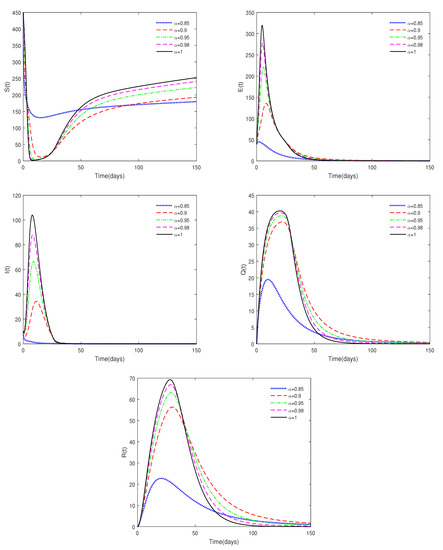
(i) Let $\mathrm{\Lambda }=1.12$, $\beta =0.018$, and $b=1$. In this case, we obtain $R_0=0.9062<1$. From Figure 1 we find that the disease-free equilibrium $E_0$ of system (1) is always locally asymptotically stable for different values of α ($\alpha =0.85,0.9,0.95,0.98,1$), which indicates that the disease will eventually die out.

Figure 1. The time series of system (1), with $R_0=0.9062<1$.

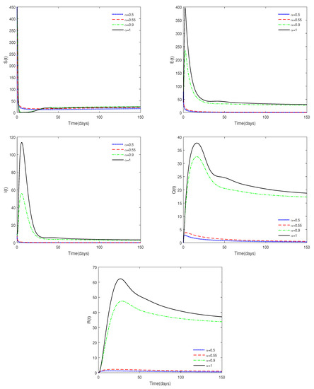
(ii) Let $\mathrm{\Lambda }=1$, $\beta =0.06$, and $b=4$. In this case, we obtain $R_0=9.9292>1$. From Figure 2, we can see that when the value of α is relatively large ($\alpha =0.9$ or $\alpha =1$), the disease-free equilibrium $E_0$ is unstable; however, it is still asymptotically stable when the value of α is relatively small (α = 0.5 or α = 0.55). These results show the different between an integer-order system and a fractional-order system. That is to say the value of parameter α has a crucial effect on the dynamics of the system.

Figure 2. The time series of system (1), with $R_0=9.9292>1$.

Example 2.

Fix the following parameter values: $\omega =0.15$, $ϵ=0.2$, $\delta =0.1$, $c=8.5$, $\mu =0.0025$, $d=0.25$, and initial value $\left[S\right(0),E(0),I(0),Q(0),R(0\left)\right]=[450,40,10,0,0]$.

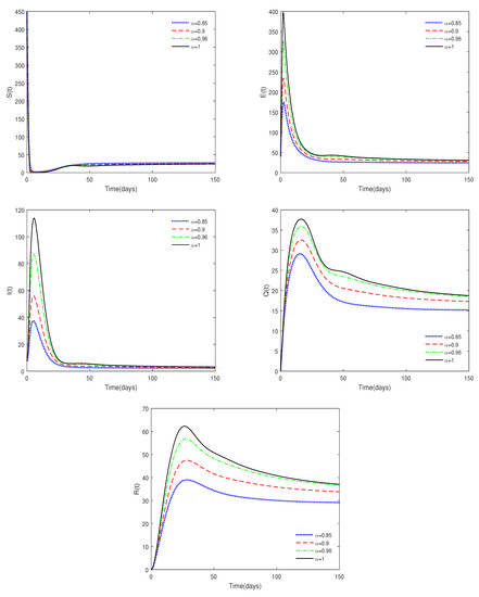
(i) Let $\mathrm{\Lambda }=1$, $\beta =0.06$ and $b=4$. In this case, we obtain $R_0=9.9292>1$. From Figure 3 we find that the endemic equilibrium $E_{*}$ is asymptotically stable for different values of α ($\alpha =0.85,0.9,0.96,1$).

Figure 3. The time series of system (1), with $R_0=9.9292>1$, and the Routh–Hurwitz conditions are satisfied.

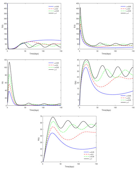
(ii) Let $\mathrm{\Lambda }=1.12$, $\beta =0.018$ and $b=1$. In this case, we obtain $R_0=3.8839>1$. Figure 4 shows that the endemic equilibrium $E_{*}$ maybe stable for some value of α ($\alpha =0.85$), or unstable for other values($\alpha =0.9,0.95,1$).

Figure 4. The time series of system (1), with $R_0=3.8839>1$ and the Routh–Hurwitz conditions are not satisfied.

From the above two examples, we find that

Remark 1.

(i) If $R_0<1$, then the disease-free equilibrium $E_0$ is always asymptotically stable for different values of α, which means that the disease will eventually die out. However, if $R_0>1$, the disease-free equilibrium $E_0$ is unstable when the value of α is relatively large; while it might be stable when the value of α is relatively small. That is to say, the values of $R_0$ and α determine the stability of equilibrium $E_0$. This shows the difference between fractional-order systems and integer-order systems.

(ii) When $R_0>1$, from Figure 3, we can see that if the Routh–Hurwitz conditions are satisfied, then the endemic equilibrium $E_{*}$ is asymptotically stable, which means that the disease will persist; however, from Figure 4, we can see that if the Routh–Hurwitz conditions are unsatisfied, the endemic equilibrium $E_{*}$ may be stable for some value of α($\alpha =0.85$), or it may be unstable for other values of α($\alpha =0.9,0.95,1$). This shows that the values of α and the basic reproduction number are crucial for the dynamics of the system.

(iii) The above results coincide with the conclusions of Theorems 3 and 4.

Example 3.

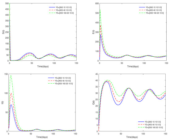
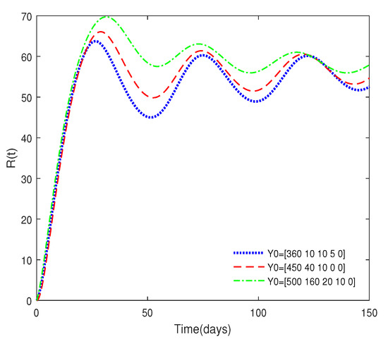
Fix the following parameter values: $\mathrm{\Lambda }=1.12$, $\beta =0.018$, $\omega =0.15$, $ϵ=0.2$, $\delta =0.1$, $b=1$, $c=8.5$, $\mu =0.0025$, $d=0.25$, and $\alpha =0.98$. In this case, we obtain $R_0=3.8839>1$. Figure 5 shows that the endemic equilibrium point $E_{*}$ is stable with different initial values $\left[S\right(0),E(0),I(0),Q(0),R(0\left)\right]=[360,10,10,5,0],[450,40,10,0,0],$$[500,160,20,10,0].$

Figure 5. The time series of system (1) with different initial values.

Example 4.

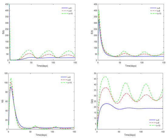
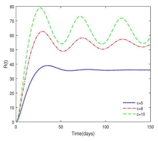
Fix the following parameter values: $\mathrm{\Lambda }=1.12$, $\beta =0.018$, $\omega =0.15$, $ϵ=0.2$, $\delta =0.1$, $b=1$, $\mu =0.0025$, and $d=0.25$. Figure 6 shows the effect of parameter c. From this figure, we can see that as the value of parameter c increases, the peaks of $Q\left(t\right)$ and $R\left(t\right)$ also increase. That is to say, if the maximum isolation rate is higher, then there are higher quarantined and recovered populations, so more medical resources are needed to control the transmission of the disease.

Figure 6. The time series of system (1) for different values of c ($c=5,8,10$).

From the above two examples, we can see that

Remark 2.

(i) From Example 3, we know that the endemic equilibrium $E_{*}$ is always stable for different initial values, which coincides with Theorem 4. That is to say, the initial data do not affect the stability of equilibriums.

(ii) The value of parameter c affects the peaks of $Q\left(t\right)$ and $R\left(t\right)$. That is to say, medical resources are important to control the transmission of the disease.

4. Discussion

In this paper, a fractional-order model for African swine fever with limited medical resources was constructed and investigated. The basic reproduction number $R_0$ and the sufficient conditions for the existence and stability of $E_0$ and $E_{*}$ were obtained.

Through qualitative analysis, we found that

◊

If $R_0<1$, then the disease-free equilibrium $E_0$ is the unique equilibrium of system (1) and it is asymptotically stable within $\mathrm{\Gamma }$.

◊

If $R_0>1$, then $E_0$ may be stable for a relatively small value of $\alpha$, or it may be unstable for a relatively large value of $\alpha$; and the endemic equilibrium $E_{*}$ appears.

◊

If $R_0>1$, then the endemic equilibrium $E_{*}$ exists and it may be stable for some values of $\alpha$ or unstable for other values of $\alpha$.

Through numerical simulation we obtained the following results:

◊

Figure 1 and Figure 2 show that the values of $\alpha$ and $R_0$ are crucial to the dynamics of the system. If $R_0<1$, then the disease-free equilibrium $E_0$ is always stable for different values of $\alpha$. If $R_0>1$, then the disease-free equilibrium $E_0$ may be stable for a relatively small value of $\alpha$; while it is unstable with a relatively large value of $\alpha$. This result shows the difference between fractional-order systems and integer-order systems.

◊

Figure 3 shows that if the Routh–Hurwitz conditions are satisfied, then the endemic equilibrium $E_{*}$ is stable for different values of $\alpha$. Figure 4 shows that the endemic equilibrium $E_{*}$ may be unstable if the Routh–Hurwitz conditions are not satisfied. Figure 5 shows that the initial values are not important to the stability of the endemic equilibrium $E_{*}$.

◊

Figure 6 shows that medical resources are important for controlling the transmission of the disease.

References

- He, C.; Zhang, B. Diagnosis of African swine fever and its prevention and control measures. Swine Ind. Sci. 2020, 37, 96–98. (In Chinese) [Google Scholar]
- Li, T.; Yu, X.; Li, F. The prevalent, diagnosis, prevention and control of African swine fever. Mod. Agric. Ind. Technol. Syst. 2019, 5, 23–25. [Google Scholar]
- Lu, Y.; Pawelek, K.; Liu, S. A stage-structured predator-prey model with predation over juvenile prey. Appl. Math. Comput. 2016, 297, 115–130. [Google Scholar] [CrossRef]
- Zhang, W.; Meng, X. Stochastic analysis of a novel nonautonomous periodic SIRI epidemic system with random disturbances. Physica A 2018, 492, 1290–1301. [Google Scholar] [CrossRef]
- Zhou, W.; Xiao, Y.; Heffernan, J. A two-thresholds policy to interrupt transmission of West Nile Virus to birds. J. Theor. Biol. 2019, 463, 22–46. [Google Scholar] [CrossRef] [PubMed]
- Lv, Y.; Pei, Y.; Yuan, R. Complete global analysis of a diffusive NPZ model with age structure in zooplankton. Nonlinear Anal. Real World Appl. 2019, 46, 274–297. [Google Scholar] [CrossRef]
- Pietschmann, J.; Guinat, C.; Beer, M.; Pronin, V.; Tauscher, K.; Petrov, A.; Keil, G.; Blome, S. Course and transmission characteristics of oral low-dose infection of domestic pigs and European wild boar with a caucasian African swine fever virus isolate. Arch. Virol. 2015, 160, 1657–1667. [Google Scholar] [CrossRef]
- Guinat, C.; Gubbins, S.; Vergne, T.; Gonzales, J.L.; Dixon, L.; Pfeiffer, D.U. Experimental pig-to-pig transmission dynamics for African swine fever virus, Georgia 2007/1 strain. Epidemiol. Infect. 2016, 144, 25–34. [Google Scholar] [CrossRef]
- Mur, L.; Sánchez-Vizcaíno, J.M.; Fernández-Carrión, E.; Jurado, C.; Rolesu, S.; Feliziani, F.; Laddomada, A.; Martínez-López, B. Understanding African swine fever infection dynamics in Sardinia using a spatially explicit transmission model in domestic pig farms. Transbound. Emerg. Dis. 2017, 65, 123–134. [Google Scholar] [CrossRef]
- Barongo, M.B.; Bishop, R.P.; Fèvre, E.M.; Knobel, D.L.; Ssematimba, A. A mathematical model that simulates control options for African swine fever virus (ASFV). PLoS ONE 2016, 11, e0158658. [Google Scholar] [CrossRef]
- Zhang, X.; Rong, X.; Li, J.; Fan, M.; Wang, Y.; Sun, X.; Huang, B.; Zhu, H. Modeling the outbreak and control of African swine fever virus in large-scale pig farms. J. Theor. Biol. 2021, 526, 110798. [Google Scholar] [CrossRef]
- Song, H.; Li, J.; Jin, Z. Nonlinear dynamic modelling and analysis of African swine fever with culling in China. Commun. Nonlinear Sci. Numer. Simul. 2023, 117, 106915. [Google Scholar] [CrossRef]
- Magin, R.; Abdullah, O.; Baleanu, D.; Zhou, X. Anomalous diffusion expressed through fractional order differential operators in the Bloch-Torrey equation. J. Magn. Reson. 2008, 190, 255–270. [Google Scholar] [CrossRef] [PubMed]
- Hilfer, R. Application of Fractional Calculus in Physics; World Scientific: Singapore, 2000. [Google Scholar]
- Laskin, N.; Zaslavsky, G. Nonlinear fractional dynamics on a lattice with long range interactions. Phys. A Stat. Mech. Its Appl. 2006, 368, 38–54. [Google Scholar] [CrossRef]
- Copot, D.; De Keyser, R.; Derom, E.; Ortigueira, M.; Ionescu, C.M. Reducing bias in fractional order impedance estimation for lung function evaluation. Biomed. Signal Process. Control 2018, 39, 74–80. [Google Scholar] [CrossRef]
- Alidousti, J.; Ghaziani, R. Spiking and bursting of a fractional order of the modified FitzHugh-Nagumo neuron model. Math. Model. Comput. Simulations 2017, 9, 390–403. [Google Scholar] [CrossRef]
- Rihan, F.; Rahman, D. Delay differential model for tumour-immune dynamics with HIV infection of CD4+ T-cells. Int. J. Comput. Math. 2013, 90, 594–614. [Google Scholar] [CrossRef]
- Shi, R.; Lu, T.; Wang, C. Dynamic analysis of a fractional-order model for HIV with drug-resistance and CTL immune response. Math. Comput. Simul. 2021, 188, 509–536. [Google Scholar] [CrossRef]
- Sweilam, N.H.; Al-Mekhlafi, S.M.; Mohammed, Z.N.; Baleanu, D. Optimal control for variable order fractional HIV/AIDS and malaria mathematical models with multi-time delay. Alex. Eng. J. 2020, 59, 3149–3162. [Google Scholar] [CrossRef]
- Ortigueira, M. Fractional calculus for scientists and engineers. Lect. Notes Electr. Eng. 2011, 84, 101–121. [Google Scholar]
- Doha, E.H.; Bhrawy, A.H.; Ezz-Eldien, S.S. A new Jacobi operational matrix: An application for solving fractional differential equations. Appl. Math. Model. 2012, 36, 4931–4943. [Google Scholar] [CrossRef]
- Muresan, C.; Ionescu, C.; Folea, S.; Keyser, R.D. Fractional order control of unstable processes: The magnetic levitation study case. Nonlinear Dyn. 2015, 80, 1761–1772. [Google Scholar] [CrossRef]
- Cao, Y.; Nikan, O.; Avazzadeh, Z. A localized meshless technique for solving 2D nonlinear integro-differential equation with multi-term kernels. Appl. Numer. Math. 2023, 183, 140–156. [Google Scholar] [CrossRef]
- Salama, F.M.; Ali, N.H.M.; Hamid, N.N.A. Fast O(N) hybrid Laplace transform-finite difference method in solving 2D time fractional diffusion equation. J. Math. Comput. Sci. 2021, 23, 110–123. [Google Scholar] [CrossRef]
- Jassim, H.K.; Hussain, M.A.S. On approximate solutions for fractional system of differential equations with Caputo-Fabrizio fractional op-erator. J. Math. Comput. Sci. 2021, 23, 58–66. [Google Scholar] [CrossRef]
- Akrama, T.; Abbasb, M.; Alia, A. A numerical study on time fractional Fisher equation using an extended cubic B-spline approximation. J. Math. Comput. Sci. 2021, 22, 85–96. [Google Scholar] [CrossRef]
- Podlubny, I. Fractional Differential Equations: An Introduction to Fractional Derivatives, Fractional Differential Equations, to Methods of Their Solution and Some of Their Applications; Academic Press: San Diego, CA, USA, 1999. [Google Scholar]
- Cui, J.; Mu, X.; Wan, H. Saturation recovery leads to multiple endemic equilibria and backward bifurcation. J. Theor. Biol. 2008, 254, 275–283. [Google Scholar] [CrossRef]
- Samko, S.; Kilbas, A.; Marichev, O. Fractional Integrals and Derivatives: Theory and Applications; Gordon and Breach Science Publishers: London, UK, 1993. [Google Scholar]
- Odibat, Z.; Shawagfeh, N. Generalized Taylors formula. Appl. Math. Comput. 2007, 186, 286–293. [Google Scholar]
- Mao, S.; Xu, R.; Li, Y. A fractional order SIRS model with standard incidence rate. J. Beihua Univ. Nat. Sci. 2012, 12, 379–382. [Google Scholar]
- Diekmann, O.; Heesterbeek, J.A.P.; Roberts, M.G. The construction of next-generation matrices for compartmental epidemic models. J. R. Soc. Interface 2010, 7, 873–885. [Google Scholar] [CrossRef]
- van Driessche, P.; Watmough, J. Reproduction numbers and sub-threshold endemic equilibria for compartmental systems of disease transmis-sion. Math. Biosci. 2002, 180, 29–48. [Google Scholar] [CrossRef] [PubMed]
- Kou, C.; Yan, Y.; Liu, J. Stability analysis for fractional differential equations and their applications in the models of HIV-1 infection. Comput. Model. Eng. Sci. 2009, 39, 301–317. [Google Scholar]
Disclaimer/Publisher’s Note: The statements, opinions and data contained in all publications are solely those of the individual author(s) and contributor(s) and not of MDPI and/or the editor(s). MDPI and/or the editor(s) disclaim responsibility for any injury to people or property resulting from any ideas, methods, instructions or products referred to in the content. |
© 2023 by the authors. Licensee MDPI, Basel, Switzerland. This article is an open access article distributed under the terms and conditions of the Creative Commons Attribution (CC BY) license (https://creativecommons.org/licenses/by/4.0/).