An Investigation on Fractal Characteristics of the Superposition of Fractal Surfaces

Abstract

In this paper, we conduct research on the fractal characteristics of the superposition of fractal surfaces from the view of fractal dimension. We give the upper bound of the lower and upper box dimensions of the graph of the sum of two bivariate continuous functions and calculate the exact values of them under some particular conditions. Further, it has been proven that the superposition of two continuous surfaces cannot keep the fractal dimensions invariable unless both of them are two-dimensional. A concrete example of a numerical experiment has been provided to verify our theoretical results. This study can be applied to the fractal analysis of metal fracture surfaces or computer image surfaces.

1. Introduction

Fractal surfaces, as a class of fractal sets in three-dimensional Euclidean space, are important research objects in fractal geometry [1]. At present, fractal surfaces have been extensively applied in a variety of academic fields, such as metal materials [2], geology [3], computer graphics [4], and so on. One of the most concerning problems is investigating how to measure the geometric complexity of a fractal surface, like the texture roughness of a metal fracture surface or a computer image surface. The fractal dimension [5] is a common measure of the geometric complexity of a surface, which can be used to describe its fractal characteristics well. It is well known that the topological dimension of a surface is two. Nevertheless, its fractal dimension increases with larger amounts of complexity or roughness, which is usually greater than its topological dimension. For instance, the fractal dimension of the relief on the earth has been found to be 2.3 in general [6]. Beyond that, many scholars have used iterative function systems ($\mathrm{IFS}$) to construct fractal surfaces that are attractors of certain $\mathrm{IFS}$. More details about fractal surfaces and relevant studies of their fractal dimensions can be found in [7,8,9,10].

In recent years, exploring the fractal dimension of the graph of fractal curves has drawn the attention of numerous researchers. There are some commonly used definitions of the fractal dimension, such as the box dimension, the packing dimension, the Hausdorff dimension and the Assouad dimension, which are denoted as ${dim}_B$, ${dim}_P$, ${dim}_H$, and ${dim}_A$ throughout this paper, respectively. Of the diverse fractal dimensions, the box dimension mainly considered in the present paper shows its advantage of relatively easy calculation. Up to now, a lot of meaningful work has been done, including fractal interpolation functions [11,12,13,14], $\alpha$-Hölder continuous functions [15,16], self-similar curves like the Von Koch curve [17,18], and some specific fractal functions like the Weierstrass function [19,20,21,22,23] and the Besicovitch function [24,25,26]. For more details of our latest work, we refer interested readers to [27,28,29,30,31,32].

Another essential issue involved recently is estimating the fractal dimension of the superposition of two fractal curves, namely, the sum of two continuous functions of one variable. This problem can be traced back to the research made first by Falconer [33], who showed that the box dimension of the sum of two continuous functions equals the greater of the box dimensions of them. On this basis, a group of academic workers has pushed this study forward and obtained a series of preliminary conclusions, whose related progress can be found in [34,35,36,37,38,39,40]. So in this paper, we shall focus on the fractal dimension of the superposition of two fractal surfaces and investigate whether it has the same result as that of fractal curves. Based on a three-dimensional Cartesian coordinate system, a fractal surface can be looked upon as a bivariate continuous function, whose fractal dimension and fractional calculus have been established in [41]. This work will contribute to enriching the theory with regards to the fractal dimension of fractal surfaces and can be applied to the research on fractal characteristics analysis of the superposition of two metal fracture surfaces or two computer image surfaces.

The outline of the remainder of this paper is organized as follows: In upcoming Section 2, we will cover the required notations, concepts, and results on the fractal dimensions of the graph of bivariate continuous functions for subsequent sections. Furthermore, in Section 3, we present our main results obtained in this paper. Firstly, we study the lower and upper box dimensions of the graph of the sum of two bivariate continuous functions and give their upper bounds. Secondly, we calculate the exact value of the lower and upper box dimensions of the graph of the sum of two bivariate continuous functions under certain particular circumstances. Thirdly, we explore some concrete situations when the two bivariate continuous functions have the box dimension or not, and we also consider the case when one of these two functions is Lipschitz. Later in Section 4, we provide a specific example and do numerical experiments to verify the theoretical results in Section 3. Finally, in Section 5, we sum up our conclusions and discuss further research in the future.

2. Preliminaries

In the present paper, all the subjects we discuss are entirely real. Given a non-empty subset $\mathcal{D}\subset {\mathbb{R}}^2$ and a bivariate function $f:\mathcal{D}\to \mathbb{R}$, the oscillation of f over the rectangular region $\mathcal{R}$ is written as

$$\mathrm{OSC}(f,\mathcal{R})=\underset{(x,y),(u,v)\in \mathcal{R}\cap \mathcal{D}}{sup}|f(x,y)-f(u,v)|$$

(1)

and the graph of $f\left(x\right)$ on $\mathcal{D}$ is defined as

$${\mathrm{G}}_f=\left\{\left(\right(x,y),f(x,y\left)\right):(x,y)\in \mathcal{D}\right\}\subseteq \mathcal{D}\times \mathbb{R}.$$

We denote $\vartheta$ as the function which is always equal to 0 on $\mathcal{D}$. Let ${∥·∥}_2$ be the usual Euclidean norm in ${\mathbb{R}}^n$. For any ${\tau }_1,{\tau }_2,\cdots ,{\tau }_n\in \mathbb{Z}$ and $\delta >0$, we call ${\prod }_{i=1}^n[{\tau }_i\delta ,({\tau }_i+1)\delta ]$ a $\delta$-coordinate cube in ${\mathbb{R}}^n$.

Below, we shall briefly introduce the definition of the box dimension. For more details about other kinds of fractal dimensions, we consult the interested readers to [1,5,33,37,42], for example.

Definition 1

([33]). Let $X\ne \varnothing$ be a bounded subset of ${\mathbb{R}}^n$ and let ${\mathcal{N}}_{\delta }\left(X\right)$ be the smallest number of δ-coordinate cubes that intersect X. Then the lower and upper box dimensions of X are defined as, respectively,

$${\underline{dim}}_B\left(X\right)=\underset{\delta \to 0}{\underline{lim}}\frac{log{\mathcal{N}}_{\delta }\left(X\right)}{-log\delta }$$

and

$${\overline{dim}}_B\left(X\right)=\underset{\delta \to 0}{\overline{lim}}\frac{log{\mathcal{N}}_{\delta }\left(X\right)}{-log\delta }.$$

If the above two are equal, we define the box dimension of X as the common value, that is,

$${dim}_B\left(X\right)=\underset{\delta \to 0}{lim}\frac{log{\mathcal{N}}_{\delta }\left(X\right)}{-log\delta }.$$

Remark 1.

The notation${\mathcal{N}}_{\delta }\left(X\right)$in Definition 1 can also be replaced by one of the following:

(1) 

The smallest number of sets of diameter at most δ that cover X;

(2) 

The smallest number of cubes of side δ that cover X;

(3) 

The largest number of disjoint balls of radius δ with centres in X;

(4) 

The smallest number of closed balls of radius δ that cover X.

Now we provide some fundamental results, which will be used in subsequent research. The forthcoming two lemmas can be essential approaches to estimating the box dimension of the graph of a bivariate continuous function.

Lemma 1

([33]). Let $f:X\subseteq {\mathbb{R}}^m\to {\mathbb{R}}^n$.

(1) 

If f is a Lipschitz map, that is,

$${∥f\left(x\right)-f\left(y\right)∥}_2\le C{∥x-y∥}_2$$

for $\forall x,y\in X$ and certain $0<C<+\infty$. Then

$$dim\left(f\left(X\right)\right)\le dim\left(X\right).$$

(2) 

If f is a bi-Lipschitz map, that is,

$$C_1{∥x-y∥}_2\le {∥f\left(x\right)-f\left(y\right)∥}_2\le C_2{∥x-y∥}_2$$

for $\forall x,y\in X$ and certain $0<C_1\le C_2<+\infty$. Then

$$dim\left(f\left(X\right)\right)=dim\left(X\right).$$

Here dim denotes any one of ${dim}_B$, ${\underline{dim}}_B$ and ${\overline{dim}}_B$.

Lemma 2

([33]). Let $f:[a,b]\times [c,d]\to \mathbb{R}$ be continuous and $0<\delta <min\left\{b-a,d-c,1\right\}$. Suppose that m and n, respectively, are the least integer greater than or equal to $\frac{b-a}{\delta }$ and $\frac{d-c}{\delta }$. Furthermore, the range of ${\mathcal{N}}_{\delta }\left({\mathrm{G}}_f\right)$ can be estimated as

$$\sum _{j=0}^{n-1}\sum _{i=0}^{m-1}max\left\{1,\mathrm{OSC}(f,{\mathcal{R}}_{i,j})·{\delta }^{-1}\right\}\le {\mathcal{N}}_{\delta }\left({\mathrm{G}}_f\right)\le \sum _{j=0}^{n-1}\sum _{i=0}^{m-1}\left\{2+\mathrm{OSC}(f,{\mathcal{R}}_{i,j})·{\delta }^{-1}\right\}$$

where ${\mathcal{R}}_{i,j}=[a+i\delta ,a+(i+1)\delta ]\times [c+j\delta ,c+(j+1)\delta ]$.

Proof. 

Since $f\left(x\right)$ is continuous on $[a,b]\times [c,d]$, the estimation of ${\mathcal{N}}_{\delta }\left({\mathrm{G}}_f\right)$ can be transformed into the oscillation of $f\left(x\right)$ on the above subregions. We note that the number of cubes of side length $\delta$ in the part above the rectangular region ${\mathcal{R}}_{i,j}$ that intersect ${\mathrm{G}}_f$ is no less than

$$max\left\{1,\mathrm{OSC}(f,{\mathcal{R}}_{i,j})·{\delta }^{-1}\right\}$$

and no more than

$$2+\mathrm{OSC}(f,{\mathcal{R}}_{i,j})·{\delta }^{-1}.$$

Summing over all the subregions just leads to the present lemma. □

The next proposition reveals several basic properties relating to the fractal dimensions of the graph of a bivariate continuous function.

Proposition 1.

Let $f:[a,b]\times [c,d]\to \mathbb{R}$ be continuous. Given a constant $r\in \mathbb{R}$, the following three statements hold.

(1) 

It holds

$$2\le {\underline{dim}}_B\left({\mathrm{G}}_f\right)\le {\overline{dim}}_B\left({\mathrm{G}}_f\right)\le 3.$$

(2) 

For a constant bivariate function $f(x,y)\equiv r$ on $[a,b]\times [c,d]$, we have

$${\underline{dim}}_B\left({\mathrm{G}}_f\right)={\overline{dim}}_B\left({\mathrm{G}}_f\right)={dim}_B\left({\mathrm{G}}_f\right)=2.$$

(3) 

If $r\ne 0$, then

$${\underline{dim}}_B\left({\mathrm{G}}_{r·f}\right)={\underline{dim}}_B\left({\mathrm{G}}_f\right)\mathrm{and}{\overline{dim}}_B\left({\mathrm{G}}_{r·f}\right)={\overline{dim}}_B\left({\mathrm{G}}_f\right).$$

Proof. 

The following arguments for (1)–(3) are all based on Definition 1, Lemmas 1 and 2.

(1)

Assume that ${max}_{(x,y)\in [a,b]\times [c,d]}\left|f(x,y)\right|=\mathcal{M}>0$. On one hand, it follows from Lemma 2 that

$$\begin{array}{cc}\hfill {\mathcal{N}}_{\delta }\left({\mathrm{G}}_f\right)& \le \sum _{j=0}^{n-1}\sum _{i=0}^{m-1}\left\{2+\mathrm{OSC}(f,{\mathcal{R}}_{i,j})·{\delta }^{-1}\right\}\hfill \\ & \le mn\left(2+2\mathcal{M}{\delta }^{-1}\right)\hfill \\ & \le 2\left((b-a){\delta }^{-1}+1\right)\left((d-c){\delta }^{-1}+1\right)\left(1+\mathcal{M}{\delta }^{-1}\right)\hfill \\ & \le 2(b-a+1)(d-c+1)(\mathcal{M}+1){\delta }^{-3}.\hfill \end{array}$$

Thus by Definition 1,

$$\begin{array}{cc}\hfill {\overline{dim}}_B\left({\mathrm{G}}_f\right)& =\underset{\delta \to 0}{\overline{lim}}\frac{log{\mathcal{N}}_{\delta }\left({\mathrm{G}}_f\right)}{-log\delta }\hfill \\ & \le \underset{\delta \to 0}{\overline{lim}}\frac{log\left[2(b-a+1)(d-c+1)(\mathcal{M}+1){\delta }^{-3}\right]}{-log\delta }\hfill \\ & =\underset{\delta \to 0}{\overline{lim}}\frac{log{\delta }^3}{log\delta }+\underset{\delta \to 0}{\overline{lim}}\frac{log\left[2(b-a+1)(d-c+1)(\mathcal{M}+1)\right]}{-log\delta }\hfill \\ & =3.\hfill \end{array}$$

On the other hand, it is observed that

$$\begin{array}{cc}\hfill {\mathcal{N}}_{\delta }\left({\mathrm{G}}_f\right)& \ge \sum _{j=0}^{n-1}\sum _{i=0}^{m-1}1\hfill \\ & =mn\hfill \\ & =\left((b-a){\delta }^{-1}+1\right)\left((d-c){\delta }^{-1}+1\right)\hfill \\ & \ge (b-a)(d-c){\delta }^{-2}.\hfill \end{array}$$

So by Definition 1, we can get

$$\begin{array}{cc}\hfill {\underline{dim}}_B\left({\mathrm{G}}_f\right)& =\underset{\delta \to 0}{\underline{lim}}\frac{log{\mathcal{N}}_{\delta }\left({\mathrm{G}}_f\right)}{-log\delta }\hfill \\ & \ge \underset{\delta \to 0}{\underline{lim}}\frac{log\left[(b-a)(d-c){\delta }^{-2}\right]}{-log\delta }\hfill \\ & =\underset{\delta \to 0}{\underline{lim}}\frac{log{\delta }^2}{log\delta }+\underset{\delta \to 0}{\underline{lim}}\frac{log\left[(b-a)(d-c)\right]}{-log\delta }\hfill \\ & =2.\hfill \end{array}$$

Obviously, we can assert from Definition 1 that ${\underline{dim}}_B\left({\mathrm{G}}_f\right)\le {\overline{dim}}_B\left({\mathrm{G}}_f\right)$, which leads to the conclusion of (1).

(2)

Note that $\mathrm{OSC}(f,{\mathcal{R}}_{i,j})=0$ when $f(x,y)\equiv r$ on $[a,b]\times [c,d]$. Consequently,

$$\begin{array}{cc}\hfill {\mathcal{N}}_{\delta }\left({\mathrm{G}}_f\right)& \le 2mn+\sum _{j=0}^{n-1}\sum _{i=0}^{m-1}\mathrm{OSC}(f,{\mathcal{R}}_{i,j})·{\delta }^{-1}\hfill \\ & \le 2\left((b-a){\delta }^{-1}+1\right)\left((d-c){\delta }^{-1}+1\right)\hfill \\ & \le 2(b-a+1)(d-c+1){\delta }^{-2}.\hfill \end{array}$$

At this time, we obtain

$$\begin{array}{cc}\hfill {\overline{dim}}_B\left({\mathrm{G}}_f\right)& =\underset{\delta \to 0}{\overline{lim}}\frac{log{\mathcal{N}}_{\delta }\left({\mathrm{G}}_f\right)}{-log\delta }\hfill \\ & \le \underset{\delta \to 0}{\overline{lim}}\frac{log\left[2(b-a+1)(d-c+1){\delta }^{-2}\right]}{-log\delta }\hfill \\ & =\underset{\delta \to 0}{\overline{lim}}\frac{log{\delta }^2}{log\delta }+\underset{\delta \to 0}{\overline{lim}}\frac{log\left[2(b-a+1)(d-c+1)\right]}{-log\delta }\hfill \\ & =2.\hfill \end{array}$$

Combining (1) of Proposition 1,

$$2\le {\underline{dim}}_B\left({\mathrm{G}}_f\right)\le {\overline{dim}}_B\left({\mathrm{G}}_f\right)\le 2.$$

That is,

$${\underline{dim}}_B\left({\mathrm{G}}_f\right)={\overline{dim}}_B\left({\mathrm{G}}_f\right)={dim}_B\left({\mathrm{G}}_f\right)=2,$$

finishing the proof of (2).

(3)

Let us define a mapping $\Gamma :{\mathrm{G}}_f\to {\mathrm{G}}_{r·f}$ by

$$\Gamma ((x,y),f(x,y))=\left((x,y),(r·f)(x,y)\right),(x,y)\in [a,b]\times [c,d]$$

for $\forall r\in \mathbb{R}\setminus \left\{0\right\}$. By using the simple properties of norm, one can show that

$$\begin{array}{cc}& {∥\Gamma \left(\right(x,y),f(x,y\left)\right)-\Gamma \left(\right(u,v),f(u,v\left)\right)∥}_2\hfill \\ & \le \sqrt{1+r^2}{∥\left((x,y),f(x,y)\right)-\left((u,v),f(u,v)\right)∥}_2\hfill \end{array}$$

and

$$\begin{array}{cc}& {∥\Gamma \left(\right(x,y),f(x,y\left)\right)-\Gamma \left(\right(u,v),f(u,v\left)\right)∥}_2\hfill \\ & \ge {\displaystyle \frac{\left|r\right|}{\sqrt{r^2+1}}}{∥\left((x,y),f(x,y)\right)-\left((u,v),f(u,v)\right)∥}_2\hfill \end{array}$$

for $\forall (x,y),(u,v)\in [a,b]\times [c,d]$. With Lemma 1, we can claim that $\Gamma$ is a bi-Lipschitz mapping and then the result of (3) holds.

□

Remark 2.

In Proposition 1, if the box dimension of ${\mathrm{G}}_f$ exists on $[a,b]\times [c,d]$, then

$$2\le {dim}_B\left({\mathrm{G}}_f\right)\le 3$$

and for $\forall r\in \mathbb{R}\setminus \left\{0\right\}$,

$${dim}_B\left({\mathrm{G}}_{r·f}\right)={dim}_B\left({\mathrm{G}}_f\right).$$

In particular, if $r=0$, we have

$${\underline{dim}}_B\left({\mathrm{G}}_{\vartheta }\right)={\overline{dim}}_B\left({\mathrm{G}}_{\vartheta }\right)={dim}_B\left({\mathrm{G}}_{\vartheta }\right)=2$$

by (2) of Proposition 1. Thus for any continuous function $f:[a,b]\times [c,d]\to \mathbb{R}$, $0·f$ must be a two-dimensional continuous function on $[a,b]\times [c,d]$.

Up to now, some particular bivariate continuous functions with non-integer fractal dimensions have been constructed. For instance, Yu [43] had given the following facts.

Example 1

([43]). For $0<\alpha <1$ and $\lambda \ge 2$, let

$$\mathcal{W}(x,y)=\sum _{j=1}^{\infty }{\lambda }^{-\alpha j}sin\left({\lambda }^{j}x\right),(x,y)\in [a,b]\times [c,d].$$

Then

$${dim}_B\left({\mathrm{G}}_{\mathcal{W}}\right)=3-\alpha .$$

Example 2

([43]). For $1<s<2$, let

$$\mathcal{B}(x,y)=\sum _{j=1}^{\infty }{\lambda }_j^{s-2}cos\left({\lambda }_{j}x\right),(x,y)\in [a,b]\times [c,d]$$

where $\frac{{\lambda }_{j+1}}{{\lambda }_j}\ge \lambda >1$ for $\forall j\in {\mathbb{N}}^{*}$. If $\frac{{\lambda }_{j+1}}{{\lambda }_j}\nearrow \infty$, then ${\underline{dim}}_B\left({\mathrm{G}}_{\mathcal{B}}\right)$ and ${\overline{dim}}_B\left({\mathrm{G}}_{\mathcal{B}}\right)$ could be any numbers satisfying

$$2\le {\underline{dim}}_B\left({\mathrm{G}}_{\mathcal{B}}\right)<{\overline{dim}}_B\left({\mathrm{G}}_{\mathcal{B}}\right)<3.$$

3. Main Results

In this section, we present our main results for the fractal dimensions in the graph of the sum of two bivariate continuous functions. For two bivariate continuous functions $f,g:[a,b]\times [c,d]\to \mathbb{R}$, our motivation is to explore the values of ${\underline{dim}}_B\left({\mathrm{G}}_{f+g}\right)$ and ${\overline{dim}}_B\left({\mathrm{G}}_{f+g}\right)$. According to Definition 1, we can notice that the estimation of ${\mathcal{N}}_{\delta }\left({\mathrm{G}}_{f+g}\right)$ is key to calculating them. Hence, we begin by investigating how to attain the range of ${\mathcal{N}}_{\delta }\left({\mathrm{G}}_{f+g}\right)$. The upcoming result about the oscillation is basic.

Theorem 1.

Let $f,g:[a,b]\times [c,d]\to \mathbb{R}$ be continuous. Furthermore, the range of $\mathrm{OSC}(f+g,{\mathcal{R}}_{i,j})$ can be estimated as

$$\begin{array}{cc}\hfill \left|\sum _{j=0}^{n-1}\sum _{i=0}^{m-1}\mathrm{OSC}(f,{\mathcal{R}}_{i,j})-\sum _{j=0}^{n-1}\sum _{i=0}^{m-1}\mathrm{OSC}(g,{\mathcal{R}}_{i,j})\right|& \le \sum _{j=0}^{n-1}\sum _{i=0}^{m-1}\mathrm{OSC}(f+g,{\mathcal{R}}_{i,j})\hfill \\ & \le \sum _{j=0}^{n-1}\sum _{i=0}^{m-1}\mathrm{OSC}(f,{\mathcal{R}}_{i,j})+\sum _{j=0}^{n-1}\sum _{i=0}^{m-1}\mathrm{OSC}(g,{\mathcal{R}}_{i,j})\hfill \end{array}$$

where $m,n,{\mathcal{R}}_{i,j}$ have been defined in Lemma 2.

Proof. 

From Equation (1), we can obtain

$$\mathrm{OSC}(-f,{\mathcal{R}}_{i,j})=\mathrm{OSC}(f,{\mathcal{R}}_{i,j})$$

(2)

and

$$\begin{array}{cc}\hfill \mathrm{OSC}(f+g,{\mathcal{R}}_{i,j})& =\underset{(x,y),(u,v)\in {\mathcal{R}}_{i,j}}{sup}|(f+g)(x,y)-(f+g)(u,v)|\hfill \\ \hfill & \le \underset{(x,y),(u,v)\in {\mathcal{R}}_{i,j}}{sup}\left\{\left|f\right(x,y)-f(u,v\left)\right|+\left|g\right(x,y)-g(u,v\left)\right|\right\}\hfill \\ \hfill & \le \underset{(x,y),(u,v)\in {\mathcal{R}}_{i,j}}{sup}|f(x,y)-f(u,v)|+\underset{(x,y),(u,v)\in {\mathcal{R}}_{i,j}}{sup}|g(x,y)-g(u,v)|\hfill \\ \hfill & \le \mathrm{OSC}(f,{\mathcal{R}}_{i,j})+\mathrm{OSC}(g,{\mathcal{R}}_{i,j}).\hfill \end{array}$$

(3)

Summing over all the rectangular regions in Equation (3) just leads to the right end of the required inequality. Furthermore, combining Equations (2) and (3), we estimate

$$\mathrm{OSC}(f,{\mathcal{R}}_{i,j})=\mathrm{OSC}(f+g-g,{\mathcal{R}}_{i,j})\le \mathrm{OSC}(f+g,{\mathcal{R}}_{i,j})+\mathrm{OSC}(g,{\mathcal{R}}_{i,j})$$

and

$$\mathrm{OSC}(g,{\mathcal{R}}_{i,j})=\mathrm{OSC}(f+g-f,{\mathcal{R}}_{i,j})\le \mathrm{OSC}(f+g,{\mathcal{R}}_{i,j})+\mathrm{OSC}(f,{\mathcal{R}}_{i,j}).$$

Thus

$$\mathrm{OSC}(f+g,{\mathcal{R}}_{i,j})\ge \left|\mathrm{OSC}(f,{\mathcal{R}}_{i,j})-\mathrm{OSC}(g,{\mathcal{R}}_{i,j})\right|.$$

(4)

Summing over all the rectangular regions in Equation (4) and using absolute value inequality, one can get the left end of our required inequality as well. □

In the light of Theorem 1 and Lemma 2, ${\mathcal{N}}_{\delta }\left({\mathrm{G}}_{f+g}\right)$ seems to have a certain relationship with ${\mathcal{N}}_{\delta }\left({\mathrm{G}}_f\right)$ and ${\mathcal{N}}_{\delta }\left({\mathrm{G}}_g\right)$. The next important theorem establishes a connection among the above three.

Theorem 2.

Let $f,g:[a,b]\times [c,d]\to \mathbb{R}$ be continuous. Furthermore, the range of ${\mathcal{N}}_{\delta }\left({\mathrm{G}}_{f+g}\right)$ can be estimated as

$$\begin{array}{c}\hfill \left|{\mathcal{N}}_{\delta }\left({\mathrm{G}}_f\right)-{\mathcal{N}}_{\delta }\left({\mathrm{G}}_g\right)\right|-\rho {\delta }^{-2}\le {\mathcal{N}}_{\delta }\left({\mathrm{G}}_{f+g}\right)\le {\mathcal{N}}_{\delta }\left({\mathrm{G}}_f\right)+{\mathcal{N}}_{\delta }\left({\mathrm{G}}_g\right)+\rho {\delta }^{-2}\end{array}$$

where $0<\delta <min\left\{b-a,d-c,1\right\}$ and $\rho =2(b-a+1)(d-c+1){\delta }^{-2}$.

Proof. 

It follows from Theorem 1 and Lemma 2 that

$$\begin{array}{cc}\hfill {\mathcal{N}}_{\delta }\left({\mathrm{G}}_{f+g}\right)& \le 2mn+{\delta }^{-1}\sum _{j=0}^{n-1}\sum _{i=0}^{m-1}\mathrm{OSC}(f+g,{\mathcal{R}}_{i,j})\hfill \\ & \le 2\left((b-a){\delta }^{-1}+1\right)\left((d-c){\delta }^{-1}+1\right)\hfill \\ & +{\delta }^{-1}\sum _{j=0}^{n-1}\sum _{i=0}^{m-1}\mathrm{OSC}(f,{\mathcal{R}}_{i,j})+{\delta }^{-1}\sum _{j=0}^{n-1}\sum _{i=0}^{m-1}\mathrm{OSC}(g,{\mathcal{R}}_{i,j})\hfill \\ & \le 2(b-a+1)(d-c+1){\delta }^{-2}+{\mathcal{N}}_{\delta }\left({\mathrm{G}}_f\right)+{\mathcal{N}}_{\delta }\left({\mathrm{G}}_g\right)\hfill \end{array}$$

and

$$\begin{array}{cc}\hfill {\mathcal{N}}_{\delta }\left({\mathrm{G}}_{f+g}\right)& \ge {\delta }^{-1}\sum _{j=0}^{n-1}\sum _{i=0}^{m-1}\mathrm{OSC}(f+g,{\mathcal{R}}_{i,j})\hfill \\ & \ge 2mn+\left|{\delta }^{-1}\sum _{j=0}^{n-1}\sum _{i=0}^{m-1}\mathrm{OSC}(f,{\mathcal{R}}_{i,j})-{\delta }^{-1}\sum _{j=0}^{n-1}\sum _{i=0}^{m-1}\mathrm{OSC}(g,{\mathcal{R}}_{i,j})\right|-2mn\hfill \\ & \ge \left|{\mathcal{N}}_{\delta }\left({\mathrm{G}}_f\right)-{\mathcal{N}}_{\delta }\left({\mathrm{G}}_g\right)\right|-2(b-a+1)(d-c+1){\delta }^{-2}.\hfill \end{array}$$

This concludes the proof of Theorem 2. □

With the help of Theorem 2, we shall prove the following several conclusions. Theorems 3 and 4 give the upper bound of ${\overline{dim}}_B\left({\mathrm{G}}_{f+g}\right)$ and ${\underline{dim}}_B\left({\mathrm{G}}_{f+g}\right)$, respectively.

Theorem 3.

Let $f,g:[a,b]\times [c,d]\to \mathbb{R}$ be continuous. Then

$${\overline{dim}}_B\left({\mathrm{G}}_{f+g}\right)\le max\left\{{\overline{dim}}_B\left({\mathrm{G}}_f\right),{\overline{dim}}_B\left({\mathrm{G}}_g\right)\right\}.$$

Proof. 

Assume that ${\overline{dim}}_B\left({\mathrm{G}}_f\right)=s_1$ and ${\overline{dim}}_B\left({\mathrm{G}}_g\right)=s_2$. Given $\forall \epsilon >0$, by Definition 1 there must exist a certain number ${\delta }_0\in (0,min\left\{b-a,d-c,1\right\})$ such that

$${\mathcal{N}}_{\delta }\left({\mathrm{G}}_f\right)\le {\delta }^{-s_1-\epsilon },$$

$${\mathcal{N}}_{\delta }\left({\mathrm{G}}_g\right)\le {\delta }^{-s_2-\epsilon }$$

for $\forall \delta \in (0,{\delta }_0]$. Then by Theorem 2, we get

$$\begin{array}{cc}\hfill {\mathcal{N}}_{\delta }\left({\mathrm{G}}_{f+g}\right)& \le {\mathcal{N}}_{\delta }\left({\mathrm{G}}_f\right)+{\mathcal{N}}_{\delta }\left({\mathrm{G}}_g\right)+\rho {\delta }^{-2}\hfill \\ & \le {\delta }^{-s_1-\epsilon }+{\delta }^{-s_2-\epsilon }+\rho {\delta }^{-2}\hfill \\ & \le \left({\delta }^{max\left\{s_1,s_2\right\}-s_1}+{\delta }^{max\left\{s_1,s_2\right\}-s_2}+\rho {\delta }^{max\left\{s_1,s_2\right\}-2+\epsilon }\right){\delta }^{-max\left\{s_1,s_2\right\}-\epsilon }\hfill \\ & \le (\rho +2){\delta }^{-max\left\{s_1,s_2\right\}-\epsilon }\hfill \end{array}$$

for $\forall \delta \in (0,{\delta }_0]$. From Definition 1, we can conclude that

$$\begin{array}{cc}\hfill {\overline{dim}}_B\left({\mathrm{G}}_{f+g}\right)& =\underset{\delta \to 0}{\overline{lim}}\frac{log{\mathcal{N}}_{\delta }\left({\mathrm{G}}_{f+g}\right)}{-log\delta }\hfill \\ & \le \underset{\delta \to 0}{\overline{lim}}\frac{log\left[(\rho +2){\delta }^{-max\left\{s_1,s_2\right\}-\epsilon }\right]}{-log\delta }\hfill \\ & =\underset{\delta \to 0}{\overline{lim}}\frac{log(\rho +2)}{-log\delta }+\underset{\delta \to 0}{\overline{lim}}\frac{log{\delta }^{max\left\{s_1,s_2\right\}+\epsilon }}{log\delta }\hfill \\ & =max\left\{s_1,s_2\right\}+\epsilon .\hfill \end{array}$$

Since the above formula is true for $\forall \epsilon >0$, we have

$${\overline{dim}}_B\left({\mathrm{G}}_{f+g}\right)\le max\left\{s_1,s_2\right\}=max\left\{{\overline{dim}}_B\left({\mathrm{G}}_f\right),{\overline{dim}}_B\left({\mathrm{G}}_g\right)\right\},$$

which completes the proof of Theorem 3. □

Theorem 4.

Let $f,g:[a,b]\times [c,d]\to \mathbb{R}$ be continuous. Then

$${\underline{dim}}_B\left({\mathrm{G}}_{f+g}\right)\le max\left\{{\overline{dim}}_B\left({\mathrm{G}}_f\right),{\underline{dim}}_B\left({\mathrm{G}}_g\right)\right\}.$$

Proof. 

Assume that

$${\overline{dim}}_B\left({\mathrm{G}}_f\right)={\alpha }_1\mathrm{and}{\underline{dim}}_B\left({\mathrm{G}}_g\right)={\alpha }_2.$$

From the definition of ${\underline{dim}}_B\left({\mathrm{G}}_g\right)$, there exists a positive subsequence ${\left\{{\delta }_{{\lambda }_k}\right\}}_{k=1}^{\infty }$ such that ${lim}_{k\to \infty }{\delta }_{{\lambda }_k}=0$ and meanwhile

$$\underset{k\to \infty }{lim}\frac{log{\mathcal{N}}_{{\delta }_{{\lambda }_k}}\left({\mathrm{G}}_g\right)}{-log{\delta }_{{\lambda }_k}}={\alpha }_2.$$

So given $\forall \epsilon >0$, there exists a ${\kappa }_1\in {\mathbb{N}}^{*}$ such that

$${\mathcal{N}}_{{\delta }_{{\lambda }_k}}\left({\mathrm{G}}_g\right)\le {\delta }_{{\lambda }_k}^{-{\alpha }_2-\epsilon }$$

(5)

when $k\ge {\kappa }_1$. Furthermore, by the definition of ${\overline{dim}}_B\left({\mathrm{G}}_f\right)$, there exists a ${\kappa }_2\in {\mathbb{N}}^{*}$ such that

$${\mathcal{N}}_{{\delta }_{{\lambda }_k}}\left({\mathrm{G}}_f\right)\le {\delta }_{{\lambda }_k}^{-{\alpha }_1-\epsilon }$$

(6)

when $k\ge {\kappa }_2$. Combining Theorem 2, Equations (5) and (6), we can obtain

$$\begin{array}{cc}\hfill {\mathcal{N}}_{{\delta }_{{\lambda }_k}}\left({\mathrm{G}}_{f+g}\right)& \le {\mathcal{N}}_{{\delta }_{{\lambda }_k}}\left({\mathrm{G}}_f\right)+{\mathcal{N}}_{{\delta }_{{\lambda }_k}}\left({\mathrm{G}}_g\right)+\rho {\delta }_{{\lambda }_k}^{-2}\hfill \\ & \le {\delta }_{{\lambda }_k}^{-{\alpha }_1-\epsilon }+{\delta }_{{\lambda }_k}^{-{\alpha }_2-\epsilon }+\rho {\delta }_{{\lambda }_k}^{-2}\hfill \\ & \le \left({\delta }_{{\lambda }_k}^{max\left\{{\alpha }_1,{\alpha }_2\right\}-{\alpha }_1}+{\delta }_{{\lambda }_k}^{max\left\{{\alpha }_1,{\alpha }_2\right\}-{\alpha }_2}+\rho {\delta }_{{\lambda }_k}^{max\left\{{\alpha }_1,{\alpha }_2\right\}-2+\epsilon }\right){\delta }_{{\lambda }_k}^{-max\left\{{\alpha }_1,{\alpha }_2\right\}-\epsilon }\hfill \\ & \le (\rho +2){\delta }_{{\lambda }_k}^{-max\left\{{\alpha }_1,{\alpha }_2\right\}-\epsilon }\hfill \end{array}$$

when $k\ge max\left\{{\kappa }_1,{\kappa }_2\right\}$. Thus by Definition 1, we have

$$\begin{array}{cc}\hfill {\underline{dim}}_B\left({\mathrm{G}}_{f+g}\right)& =\underset{\delta \to 0}{\underline{lim}}\frac{log{\mathcal{N}}_{\delta }\left({\mathrm{G}}_{f+g}\right)}{-log\delta }\hfill \\ & \le \underset{k\to \infty }{lim}\frac{log\left[(\rho +2){\delta }_{{\lambda }_k}^{-max\left\{{\alpha }_1,{\alpha }_2\right\}-\epsilon }\right]}{-log{\delta }_{{\lambda }_k}}\hfill \\ & =\underset{k\to \infty }{lim}\frac{log(\rho +2)}{-log{\delta }_{{\lambda }_k}}+\underset{k\to \infty }{lim}\frac{log{\delta }_{{\lambda }_k}^{max\left\{{\alpha }_1,{\alpha }_2\right\}+\epsilon }}{log{\delta }_{{\lambda }_k}}\hfill \\ & =max\left\{{\alpha }_1,{\alpha }_2\right\}+\epsilon .\hfill \end{array}$$

In the light of the arbitrariness of $\epsilon$, we immediately get our required result. □

Under certain particular circumstances, the previous two formulae could take an equal sign, shown in the undermentioned two theorems.

Theorem 5.

Let $f,g:[a,b]\times [c,d]\to \mathbb{R}$ be continuous. If

$${\overline{dim}}_B\left({\mathrm{G}}_f\right)\ne {\overline{dim}}_B\left({\mathrm{G}}_g\right),$$

then

$${\overline{dim}}_B\left({\mathrm{G}}_{f+g}\right)=max\left\{{\overline{dim}}_B\left({\mathrm{G}}_f\right),{\overline{dim}}_B\left({\mathrm{G}}_g\right)\right\}.$$

Proof. 

Let $H=f+g$. Without loss of generality, we can assume that

$${\overline{dim}}_B\left({\mathrm{G}}_f\right)>{\overline{dim}}_B\left({\mathrm{G}}_g\right).$$

(7)

Suppose that

$${\overline{dim}}_B\left({\mathrm{G}}_H\right)\ne max\left\{{\overline{dim}}_B\left({\mathrm{G}}_f\right),{\overline{dim}}_B\left({\mathrm{G}}_g\right)\right\}={\overline{dim}}_B\left({\mathrm{G}}_f\right).$$

From Theorem 3, it follows that

$${\overline{dim}}_B\left({\mathrm{G}}_H\right)<{\overline{dim}}_B\left({\mathrm{G}}_f\right).$$

(8)

Then combining Equations (7) and (8), we have

$$\begin{array}{cc}\hfill {\overline{dim}}_B\left({\mathrm{G}}_{H-g}\right)& ={\overline{dim}}_B\left({\mathrm{G}}_f\right)\hfill \\ & >max\left\{{\overline{dim}}_B\left({\mathrm{G}}_H\right),{\overline{dim}}_B\left({\mathrm{G}}_g\right)\right\}\hfill \\ & =max\left\{{\overline{dim}}_B\left({\mathrm{G}}_H\right),{\overline{dim}}_B\left({\mathrm{G}}_{-g}\right)\right\},\hfill \end{array}$$

which is a contradiction to Theorem 3. Therefore, we can conclude that

$${\overline{dim}}_B\left({\mathrm{G}}_{f+g}\right)={\overline{dim}}_B\left({\mathrm{G}}_H\right)=max\left\{{\overline{dim}}_B\left({\mathrm{G}}_f\right),{\overline{dim}}_B\left({\mathrm{G}}_g\right)\right\}.$$

This means the conclusion of Theorem 5 holds. □

Theorem 6.

Let $f,g:[a,b]\times [c,d]\to \mathbb{R}$ be continuous. If

$$max\left\{{\underline{dim}}_B\left({\mathrm{G}}_f\right),{\underline{dim}}_B\left({\mathrm{G}}_g\right)\right\}>min\left\{{\overline{dim}}_B\left({\mathrm{G}}_f\right),{\overline{dim}}_B\left({\mathrm{G}}_g\right)\right\},$$

then

$${\underline{dim}}_B\left({\mathrm{G}}_{f+g}\right)=max\left\{{\underline{dim}}_B\left({\mathrm{G}}_f\right),{\underline{dim}}_B\left({\mathrm{G}}_g\right)\right\}.$$

Proof. 

Without loss of generality, we suppose that

$${\eta }_1={\underline{dim}}_B\left({\mathrm{G}}_g\right)>{\overline{dim}}_B\left({\mathrm{G}}_f\right)={\eta }_2.$$

At this time, we know that

$$max\left\{{\underline{dim}}_B\left({\mathrm{G}}_f\right),{\underline{dim}}_B\left({\mathrm{G}}_g\right)\right\}={\eta }_1>{\eta }_2=min\left\{{\overline{dim}}_B\left({\mathrm{G}}_f\right),{\overline{dim}}_B\left({\mathrm{G}}_g\right)\right\}.$$

From Theorem 4, it follows that

$${\underline{dim}}_B\left({\mathrm{G}}_{f+g}\right)\le max\left\{{\overline{dim}}_B\left({\mathrm{G}}_f\right),{\underline{dim}}_B\left({\mathrm{G}}_g\right)\right\}={\eta }_1.$$

(9)

Next, we prove that ${\underline{dim}}_B\left({\mathrm{G}}_{f+g}\right)\ge {\eta }_1$ as below. By the definition of ${\underline{dim}}_B\left({\mathrm{G}}_g\right)$ and ${\overline{dim}}_B\left({\mathrm{G}}_f\right)$, given $\forall \epsilon \in \left(0,\frac{{\eta }_1-{\eta }_2}{2}\right)$, there exists a ${\delta }_1\in (0,min\left\{b-a,d-c,1\right\})$ such that

$${\mathcal{N}}_{\delta }\left({\mathrm{G}}_f\right)\le {\delta }^{-{\eta }_2-\epsilon }<{\delta }^{-{\eta }_1+\epsilon }\le {\mathcal{N}}_{\delta }\left({\mathrm{G}}_g\right)$$

for $\forall \delta \in (0,{\delta }_1]$. Note that ${\eta }_1-{\eta }_2-2\epsilon >0$ and ${\eta }_1-2-\epsilon >0$, thus there exists a ${\delta }_2\in (0,min\left\{b-a,d-c,1\right\})$ such that

$${\delta }^{{\eta }_1-{\eta }_2-2\epsilon }\le \frac{1}{3}\mathrm{and}{\delta }^{{\eta }_1-2-\epsilon }\le \frac{1}{3\rho }$$

for $\forall \delta \in (0,{\delta }_2]$. Furthermore, by Theorem 2, we estimate

$$\begin{array}{cc}\hfill {\mathcal{N}}_{\delta }\left({\mathrm{G}}_{f+g}\right)& \ge \left|{\mathcal{N}}_{\delta }\left({\mathrm{G}}_f\right)-{\mathcal{N}}_{\delta }\left({\mathrm{G}}_g\right)\right|-\rho {\delta }^{-2}\hfill \\ & \ge {\delta }^{-{\eta }_1+\epsilon }-{\delta }^{-{\eta }_2-\epsilon }-\rho {\delta }^{-2}\hfill \\ & \ge \left(1-{\delta }^{{\eta }_1-{\eta }_2-2\epsilon }-\rho {\delta }^{{\eta }_1-2-\epsilon }\right){\delta }^{-{\eta }_1+\epsilon }\hfill \\ & \ge {\displaystyle \frac{1}{3}}{\delta }^{-{\eta }_1+\epsilon }\hfill \end{array}$$

for $\forall \delta \in (0,min\left\{{\delta }_1,{\delta }_2\right\}]$. Consequently, one can get

$${\underline{dim}}_B\left({\mathrm{G}}_{f+g}\right)=\underset{\delta \to 0}{\underline{lim}}\frac{log{\mathcal{N}}_{\delta }\left({\mathrm{G}}_{f+g}\right)}{-log\delta }\ge \underset{\delta \to 0}{\underline{lim}}\frac{log\frac{1}{3}{\delta }^{-{\eta }_1+\epsilon }}{-log\delta }={\eta }_1-\epsilon$$

by Definition 1. Since $\epsilon$ in the above formula is arbitrary, we have ${\underline{dim}}_B\left({\mathrm{G}}_{f+g}\right)\ge {\eta }_1$. Combining Equation (9), we just obtain the required result. □

Now we shall deal with some concrete examples of the fractal dimensions of the graph of the sum of two bivariate continuous functions. To this end, we first need to state the definition of function spaces as follows.

Definition 2.

Spaces of bivariate continuous functions.

(1) 

Let ${\mathcal{S}}^d$ be the space of all bivariate continuous functions whose box dimension exists and is equal to d on $[a,b]\times [c,d]$ as $2\le d\le 3$. Namely, ${\mathcal{S}}^d$ is the space of d-dimensional bivariate continuous functions on $[a,b]\times [c,d]$.

(2) 

Let ${\mathcal{S}}_{d_1}^{d_2}$ as the space of all bivariate continuous functions whose box dimension does not exist on $[a,b]\times [c,d]$. Here $d_1,d_2$ are the lower and upper box dimensions of the function on $[a,b]\times [c,d]$ as $2\le d_1<d_2\le 3$, respectively.

Below, we start with the case when the two bivariate continuous functions have a different box dimension.

Proposition 2.

Let $f(x,y)\in {\mathcal{S}}^{d_1}$ and $g(x,y)\in {\mathcal{S}}^{d_2}$. If $d_1\ne d_2$, then

$$f(x,y)+g(x,y)\in {\mathcal{S}}^{max\left\{d_1,d_2\right\}}.$$

Proof. 

Without loss of generality, suppose that $d_1>d_2$. At this time, we observe that

$${\underline{dim}}_B\left({\mathrm{G}}_g\right)={\overline{dim}}_B\left({\mathrm{G}}_g\right)<{\underline{dim}}_B\left({\mathrm{G}}_f\right)={\overline{dim}}_B\left({\mathrm{G}}_f\right).$$

Then it follows from Theorems 5 and 6 that

$${\overline{dim}}_B\left({\mathrm{G}}_{f+g}\right)=max\left\{{\overline{dim}}_B\left({\mathrm{G}}_f\right),{\overline{dim}}_B\left({\mathrm{G}}_g\right)\right\}=max\left\{d_1,d_2\right\}$$

and

$${\underline{dim}}_B\left({\mathrm{G}}_{f+g}\right)=max\left\{{\underline{dim}}_B\left({\mathrm{G}}_f\right),{\underline{dim}}_B\left({\mathrm{G}}_g\right)\right\}=max\left\{d_1,d_2\right\}.$$

That is,

$${dim}_B\left({\mathrm{G}}_{f+g}\right)=max\left\{d_1,d_2\right\},$$

completing the proof of Proposition 2. □

The upcoming two corollaries discuss a few situations when at least one of two bivariate continuous functions does not have the box dimension on $[a,b]\times [c,d]$. These results can easily be obtained from Theorems 5 and 6, with their proofs omitted.

Corollary 1.

Let $f(x,y)\in {\mathcal{S}}_{d_1}^{d_2}$ and $g(x,y)\in {\mathcal{S}}^d$.

(1) 

If $d_1<d_2<d$,

$$f(x,y)+g(x,y)\in {\mathcal{S}}^d.$$

(2) 

If $d<d_1<d_2$,

$$f(x,y)+g(x,y)\in {\mathcal{S}}_{d_1}^{d_2}.$$

Corollary 2.

Let $f(x,y)\in {\mathcal{S}}_{d_1}^{d_2}$, $g(x,y)\in {\mathcal{S}}_{d_3}^{d_4}$.

(1) 

If $d_1<d_2<d_3<d_4$,

$$f(x,y)+g(x,y)\in {\mathcal{S}}_{d_3}^{d_4}.$$

(2) 

If $d_3<d_4<d_1<d_2$,

$$f(x,y)+g(x,y)\in {\mathcal{S}}_{d_1}^{d_2}.$$

If the two bivariate continuous functions have the same box dimension d, the result will become more complicated. Here we discuss two situations according to whether d equals to two or not. If $d\ne 2$, we can arrive at the following two conclusions.

Proposition 3.

Let $f(x,y),g(x,y)\in {\mathcal{S}}^d$ for $2<d\le 3$. If the box dimension of ${\mathrm{G}}_{f+g}$ exists, then

$$f(x,y)+g(x,y)\in \underset{t\in [2,d]}{⨁}{\mathcal{S}}^t.$$

Proof. 

Firstly, let

$$f(x,y)=-g(x,y)+\mathcal{W}(x,y)$$

where $\mathcal{W}(x,y)$ is the function given in Example 1 and ${dim}_B\left({\mathrm{G}}_{\mathcal{W}}\right)=3-\alpha$ could be any number belonging to $(2,d)$ by choosing suitable $\alpha$. Furthermore, from Propositions 1 and 2, it follows that

$$\begin{array}{cc}\hfill {dim}_B\left({\mathrm{G}}_f\right)& ={dim}_B\left({\mathrm{G}}_{-g+\mathcal{W}}\right)\hfill \\ \hfill & =max\left\{{dim}_B\left({\mathrm{G}}_g\right),{dim}_B\left({\mathrm{G}}_{\mathcal{W}}\right)\right\}\hfill \\ \hfill & =max\left\{d,3-\alpha \right\}\hfill \\ \hfill & =d.\hfill \end{array}$$

Secondly, let

$$f(x,y)=-g(x,y)+H(x,y)$$

where $H\left(x\right)\in {\mathcal{S}}^2$. At this time,

$${dim}_B\left({\mathrm{G}}_f\right)=max\left\{{dim}_B\left({\mathrm{G}}_g\right),{dim}_B\left({\mathrm{G}}_H\right)\right\}=max\left\{d,2\right\}=d.$$

Thirdly, let $f(x,y)=g(x,y)$. Furthermore, we know from Proposition 1 that

$${dim}_B\left({\mathrm{G}}_{f+g}\right)={dim}_B\left({\mathrm{G}}_{2f}\right)={dim}_B\left({\mathrm{G}}_f\right)=d.$$

According to the above discussion, we just finish the proof of the present proposition. □

Proposition 4.

Let $f(x,y),g(x,y)\in {\mathcal{S}}^d$ for $2<d\le 3$. If the box dimension of ${\mathrm{G}}_{f+g}$ does not exist, then

$$f(x,y)+g(x,y)\in \underset{\begin{array}{c}{t}_1,t_2\in [2,d)\\ t_1<t_2\end{array}}{⨁}{\mathcal{S}}_{t_1}^{t_2}.$$

Proof. 

Let

$$f(x,y)=-g(x,y)+\mathcal{B}(x,y)$$

where $\mathcal{B}(x,y)$ is the function given in Example 2 and ${\underline{dim}}_B\left({\mathrm{G}}_{\mathcal{B}}\right),{\overline{dim}}_B\left({\mathrm{G}}_{\mathcal{B}}\right)$ could be any numbers satisfying

$$2\le {\underline{dim}}_B\left({\mathrm{G}}_{\mathcal{B}}\right)<{\overline{dim}}_B\left({\mathrm{G}}_{\mathcal{B}}\right)<d\le 3.$$

(10)

From Theorems 5 and 6, we can get

$${\overline{dim}}_B\left({\mathrm{G}}_f\right)={\overline{dim}}_B\left({\mathrm{G}}_{-g+\mathcal{B}}\right)=max\left\{{\overline{dim}}_B\left({\mathrm{G}}_g\right),{\overline{dim}}_B\left({\mathrm{G}}_{\mathcal{B}}\right)\right\}=d$$

and

$${\underline{dim}}_B\left({\mathrm{G}}_f\right)={\underline{dim}}_B\left({\mathrm{G}}_{-g+\mathcal{B}}\right)={\underline{dim}}_B\left({\mathrm{G}}_g\right)=d,$$

which implies that

$${dim}_B\left({\mathrm{G}}_f\right)=d.$$

Then by Equation (10), we just obtain our required result. □

If $d=2$, the next result manifests that the sum of two two-dimensional bivariate continuous functions can keep the fractal dimension closed.

Theorem 7.

Let $f(x,y),g(x,y)\in {\mathcal{S}}^2$. Then $f(x,y)+g(x,y)\in {\mathcal{S}}^2$.

Proof. 

From Theorem 3, it follows that

$${\overline{dim}}_B\left({\mathrm{G}}_{f+g}\right)\le max\left\{{\overline{dim}}_B\left({\mathrm{G}}_f\right),{\overline{dim}}_B\left({\mathrm{G}}_g\right)\right\}=2.$$

Combining (1) of Proposition 1, we obtain

$$2\le {\underline{dim}}_B\left({\mathrm{G}}_{f+g}\right)\le {\overline{dim}}_B\left({\mathrm{G}}_{f+g}\right)\le 2.$$

Thus

$${dim}_B\left({\mathrm{G}}_{f+g}\right)=2,$$

namely, $f(x,y)+g(x,y)\in {\mathcal{S}}^2$. □

In particular, if one of the two bivariate continuous functions is Lipschitz, we have the following assertion.

Theorem 8.

Let $f,g:[a,b]\times [c,d]\to \mathbb{R}$ be continuous. If g is Lipschitz on $[a,b]\times [c,d]$, then

$$dim\left({\mathrm{G}}_{f+g}\right)=dim\left({\mathrm{G}}_f\right)$$

where dim denotes any one of ${dim}_H$, ${dim}_P$, ${dim}_A$, ${dim}_B$, ${\underline{dim}}_B$ and ${\overline{dim}}_B$.

Proof. 

Let us define a map ${\rm Y}:{\mathrm{G}}_f\to {\mathrm{G}}_{f+g}$ by

$${\rm Y}((x,y),f(x,y))=\left((x,y),f(x,y)+g(x,y)\right),(x,y)\in [a,b]\times [c,d].$$

Since g is Lipschitz on $[a,b]\times [c,d]$, let

$$\mathrm{L}=\underset{(x,y),(u,t)\in [a,b]\times [c,d]}{sup}\frac{\left|g(x,y)-g(u,t)\right|}{{∥(x,y)-(u,t)∥}_2}<+\infty .$$

For $\forall (x,y),(u,t)\in [a,b]\times [c,d]$, on one hand,

$$\begin{array}{cc}& {∥{\rm Y}\left(\right(x,y),f(x,y\left)\right)-{\rm Y}\left(\right(u,t),f(u,t\left)\right)∥}_2^2\hfill \\ \hfill =& {∥\left((x,y),f(x,y)+g(x,y)\right)-\left((u,t),f(u,t)+g(u,t)\right)∥}_2^2\hfill \\ \hfill =& {∥(x,y)-(u,t)∥}_2^2+{|\left(f(x,y)-f(u,t)\right)+\left(g(x,y)-g(u,t)\right)|}^2\hfill \\ \hfill \le & {∥(x,y)-(u,t)∥}_2^2{+2|f(x,y)-f(u,t)|}^2+2{|g(x,y)-g(u,t)|}^2\hfill \\ \hfill \le & {∥(x,y)-(u,t)∥}_2^2+2{|f(x,y)-f(u,t)|}^2+2{\mathrm{L}}^2{∥(x,y)-(u,t)∥}_2^2\hfill \\ \hfill =& \left(1+2{\mathrm{L}}^2\right){∥(x,y)-(u,t)∥}_2^2+2{|f(x,y)-f(u,t)|}^2\hfill \\ \hfill \le & \left(3+2{\mathrm{L}}^2\right){∥((x,y),f(x,y))-\left((u,t),f(u,t)\right)∥}_2^2.\hfill \end{array}$$

On the other hand,

$$\begin{array}{cc}& {∥((x,y),f(x,y))-\left((u,t),f(u,t)\right)∥}_2^2\hfill \\ \hfill =& {∥(x,y)-(u,t)∥}_2^2+{|f(x,y)-f(u,t)|}^2\hfill \\ \hfill =& {∥(x,y)-(u,t)∥}_2^2+{\left|\left(f(x,y)-f(u,t)\right)+\left(g(x,y)-g(u,t)\right)-\left(g(x,y)-g(u,t)\right)\right|}^2\hfill \\ \hfill \le & {∥(x,y)-(u,t)∥}_2^2+2{\left|\left(f(x,y)-f(u,t)\right)+\left(g(x,y)-g(u,t)\right)\right|}^2+2{|g(x,y)-g(u,t)|}^2\hfill \\ \hfill \le & {∥(x,y)-(u,t)∥}_2^2+2{\left|\left(f(x,y)-f(u,t)\right)+\left(g(x,y)-g(u,t)\right)\right|}^2+2{\mathrm{L}}^2{∥(x,y)-(u,t)∥}_2^2\hfill \\ \hfill =& \left(1+2{\mathrm{L}}^2\right){∥(x,y)-(u,t)∥}_2^2+2{\left|\left(f(x,y)-f(u,t)\right)+\left(g(x,y)-g(u,t)\right)\right|}^2\hfill \\ \hfill \le & \left(3+2{\mathrm{L}}^2\right){∥{\rm Y}\left(\right(x,y),f(x,y\left)\right)-{\rm Y}\left(\right(u,t),f(u,t\left)\right)∥}_2^2.\hfill \end{array}$$

Then by the above two inequalities, we can obtain

$$\begin{array}{cc}\hfill C_1{∥((x,y),f(x,y))-\left((u,t),f(u,t)\right)∥}_2\le & {∥{\rm Y}\left(\right(x,y),f(x,y\left)\right)-{\rm Y}\left(\right(u,t),f(u,t\left)\right)∥}_2\hfill \\ \hfill & \le C_2{∥((x,y),f(x,y))-\left((u,t),f(u,t)\right)∥}_2\hfill \end{array}$$

where $C_1={\displaystyle \frac{1}{\sqrt{3+2{\mathrm{L}}^2}}}$ and $C_2=\sqrt{3+2{\mathrm{L}}^2}$ satisfying $0<C_1<C_2<+\infty$. This means that ${\rm Y}$ is a bi-Lipschitz map. With Lemma 1, we just get our required result. □

4. Examples

In this section, we give a concrete example to verify the result acquired in Section 3.

Example 3.

For $0<\alpha <1$, let

$${\mathcal{W}}^{*}(x,y)=\sum _{j=1}^{\infty }{2}^{-\alpha j}sin\left(2^{j}x\right),(x,y)\in [0,1]\times [0,1]$$

and

$${\mathcal{B}}^{*}(x,y)=\sum _{j=1}^{\infty }{\left(2j\right)}^{-\frac{9}{10}\times 2^j}cos\left({\left(2j\right)}^{2^j}x\right),(x,y)\in [0,1]\times [0,1].$$

By [43], we have

$${dim}_B\left({\mathrm{G}}_{{\mathcal{W}}^{*}}\right)=3-\alpha ,{\underline{dim}}_B\left({\mathrm{G}}_{{\mathcal{B}}^{*}}\right)=\frac{39}{19}\mathrm{and}{\overline{dim}}_B\left({\mathrm{G}}_{{\mathcal{B}}^{*}}\right)=\frac{21}{10}.$$

If $0<\alpha <\frac{9}{10}$, it follows from Corollary 1 that

$${dim}_B\left({\mathrm{G}}_{{\mathcal{W}}^{*}+{\mathcal{B}}^{*}}\right)={dim}_B\left({\mathrm{G}}_{{\mathcal{W}}^{*}}\right)=3-\alpha .$$

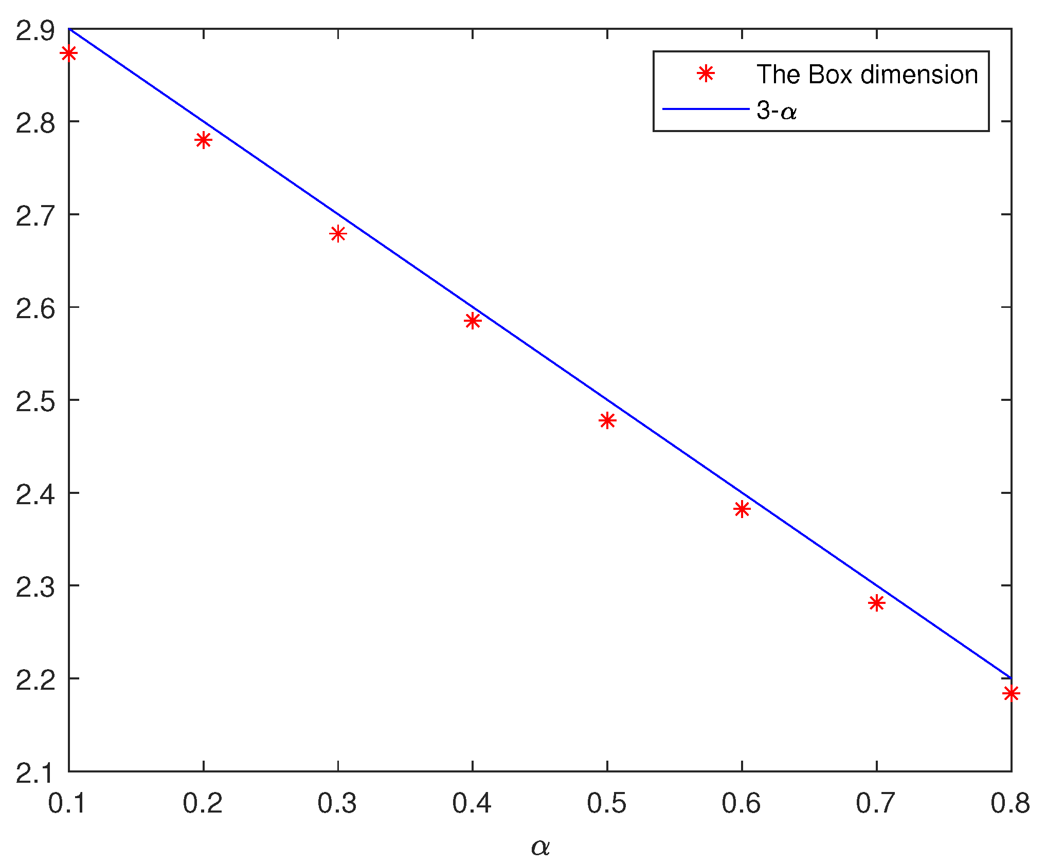
Now we show several graphs and numerical results for Example 3. Figure 1 indicates the graph of ${\mathcal{W}}^{*}$ when $\alpha =0.5$. Figure 2 denotes the graph of ${\mathcal{B}}^{*}$. Figure 3 represents the graph of ${\mathcal{W}}^{*}+{\mathcal{B}}^{*}$. Let $\alpha$ be 0.1, 0.2, 0.3, 0.4, 0.5, 0.6, 0.7, and 0.8, respectively. Table 1 presents the corresponding numerical results for the box dimension of the graph by using the computing methods stated in [44]. In addition, Figure 4 supports our theoretical results gained in Section 3, where the minor deviation may be rendered by the approximation of the computer process.

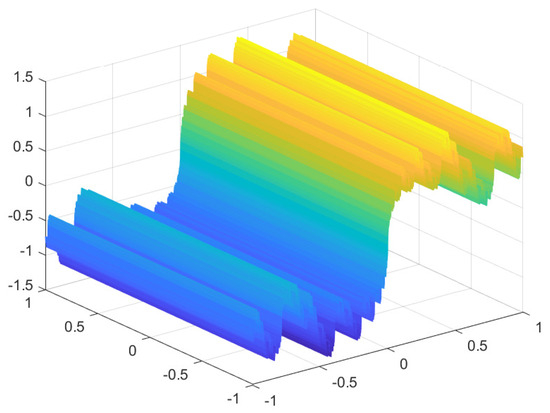
Figure 1. The graph of ${\mathcal{W}}^{*}$.

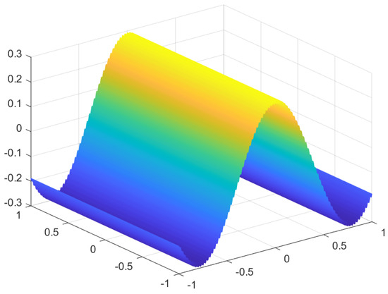
Figure 2. The graph of ${\mathcal{B}}^{*}$.

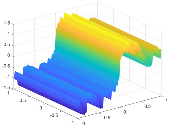
Figure 3. The graph of ${\mathcal{B}}^{*}+{\mathcal{W}}^{*}$.

Table 1. Connection between $\alpha$ and ${dim}_B\left({\mathrm{G}}_{{\mathcal{W}}^{*}+{\mathcal{B}}^{*}}\right)$.

$\mathit{\alpha }$	${dim}_{\mathit{B}}\left({\mathbf{G}}_{{\mathcal{W}}^{\mathbf{*}}+{\mathcal{B}}^{\mathbf{*}}}\right)$
0.1	2.8736
0.2	2.7801
0.3	2.6792
0.4	2.5853
0.5	2.4779
0.6	2.3825
0.7	2.2814
0.8	2.1840

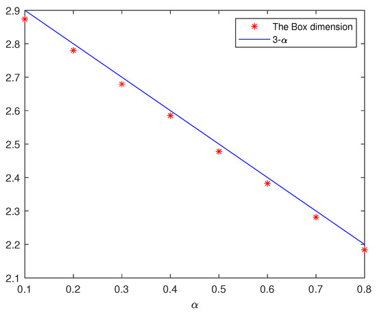
Figure 4. Comparison between numerical results and theoretical results.

5. Conclusions

In this last section, we sum up conclusions obtained in this paper.

5.1. Conclusions and Remarks

Throughout the present paper, we mainly focus on the fractal dimensions of the graph of the superposition of two continuous surfaces f and g on $[a,b]\times [c,d]$ with certain lower and upper box dimensions. Our main conclusions can be summarized in the following several aspects:

(1)

${\overline{dim}}_B\left({\mathrm{G}}_{f+g}\right)\le max\left\{{\overline{dim}}_B\left({\mathrm{G}}_f\right),{\overline{dim}}_B\left({\mathrm{G}}_g\right)\right\}$.

(2)

${\underline{dim}}_B\left({\mathrm{G}}_{f+g}\right)\le max\left\{{\overline{dim}}_B\left({\mathrm{G}}_f\right),{\underline{dim}}_B\left({\mathrm{G}}_g\right)\right\}$.

(3)

When

$${\overline{dim}}_B\left({\mathrm{G}}_f\right)\ne {\overline{dim}}_B\left({\mathrm{G}}_g\right),$$

we prove that

$${\overline{dim}}_B\left({\mathrm{G}}_{f+g}\right)=max\left\{{\overline{dim}}_B\left({\mathrm{G}}_f\right),{\overline{dim}}_B\left({\mathrm{G}}_g\right)\right\}.$$

(4)

When

$$max\left\{{\underline{dim}}_B\left({\mathrm{G}}_f\right),{\underline{dim}}_B\left({\mathrm{G}}_g\right)\right\}>min\left\{{\overline{dim}}_B\left({\mathrm{G}}_f\right),{\overline{dim}}_B\left({\mathrm{G}}_g\right)\right\},$$

we prove that

$${\underline{dim}}_B\left({\mathrm{G}}_{f+g}\right)=max\left\{{\underline{dim}}_B\left({\mathrm{G}}_f\right),{\underline{dim}}_B\left({\mathrm{G}}_g\right)\right\}.$$

(5)

It has been proven that the superposition of two continuous surfaces cannot keep the fractal dimensions invariable unless both of them are two-dimensional.

(6)

It has been proven that the fractal dimensions of the graph of the sum of a bivariate continuous function and a bivariate Lipschitz function equal the fractal dimensions of the graph of the former. That is, a bivariate Lipschitz function can be absorbed by any other bivariate continuous function in the sense of fractal dimensions.

Moreover, it is worth mentioning that the previous results can be extended to any closed regain $\mathcal{D}\subset {\mathbb{R}}^2$. In other words, all the results attained in the present paper still hold for two continuous surfaces f and g defined on $\mathcal{D}$.

5.2. Applications in Other Fields

In recent years, estimation of the fractal dimensions of the superposition of continuous surfaces has been widely applied in various fields, such as metal materials, computer graphics, and more.

In metal materials, the fracture surface topography with regards to the fatigue of metals can be studied by fractal characteristics, which can be found in [45,46]. Furthermore, fractal dimension is closely related to the parameters of the areal surface of metals, as shown in [2]. As is known to all, there are a good deal of approaches to calculating fractal dimensions, and the results under different resolutions and methods will be slightly different. This work principally investigates how to calculate fractal dimensions by counting boxes and how to estimate the fractal dimensions of the superposition of two fractal surfaces, which can be applied to research on fracture surface topography regarding the fatigue of metals.

In computer graphics, texture roughness is an important visual feature of computer images, which is of great significance to image analysis, recognition, and interpretation. A lot of research work has been done on texture analysis and many methods for measuring and describing texture roughness have been proposed (see [47,48,49,50], for example). Fractal dimension is one of the mostly used tools to describe the texture roughness of image surfaces, namely, the complexity of image gray surfaces, which can be a representation of image stability. The higher the fractal dimension, the more complex the surface, and then the coarser the image. The results in this paper can also contribute to calculating the fractal dimensions of the surface of the superposition of two computer images.

Besides, there are a lot of other potential applications of the theory of fractal surfaces like geology [3], oceanography [51], geosciences [52,53,54] and so on. Relevant interested researchers can further explore these applications in the future.

5.3. Further Research

In this paper, there are still some points worthy of improvement and further consideration in the future. Here we present them and put forward several open questions, including the following:

(1)

This work only deals with cases when the two bivariate continuous functions have a different upper box dimension and the lower box dimension of one function is larger than the upper box dimension of the other one. People could further explore the other situations later.

Question 1. Suppose that $f(x,y)\in {\mathcal{S}}_{d_1}^{d_2}$, $g(x,y)\in {\mathcal{S}}_{d_3}^{d_4}$. What is ${\overline{dim}}_B\left({\mathrm{G}}_{f+g}\right)$ when $d_2=d_4$ and what is ${\underline{dim}}_B\left({\mathrm{G}}_{f+g}\right)$ when $d_2\ge d_3$?

(2)

In the present paper, we only focus on the box dimension of the graph of the sum of two bivariate continuous functions. Therefore, other kinds of fractal dimensions, such as the packing dimension, the Hausdorff dimension, and the Assouad dimension, could be further considered for this problem.

Question 2. Let $f(x,y),g(x,y):[a,b]\times [c,d]\to \mathbb{R}$ be continuous. What can ${dim}_P\left({\mathrm{G}}_{f+g}\right)$, ${dim}_H\left({\mathrm{G}}_{f+g}\right)$ and ${dim}_A\left({\mathrm{G}}_{f+g}\right)$ be, respectively?

(3)

This study is only about bivariate continuous functions, which could be generalized to continuous functions of n variables in the future.

Question 3. Let $f\left(\mathbf{x}\right),g\left(\mathbf{x}\right):{\prod }_{i=1}^n[a_i,b_i]\to \mathbb{R}$ be continuous. What can the fractal dimensions of ${\mathrm{G}}_{f+g}$ be?

(4)

Apart from this, people could further investigate the fractal dimensions of the graph of bivariate continuous functions under other operations.

Question 4. Let $f(x,y),g(x,y):[a,b]\times [c,d]\to \mathbb{R}$ be continuous. What can the fractal dimensions of ${\mathrm{G}}_{f·g}$ be?

References

- Mandelbrot, B.B. The Fractal Geometry of Nature; Freeman: Sanfrancisco, CA, USA, 1982. [Google Scholar]
- Mandelbrot, B.B.; Passoja, D.E.; Paullay, A.J. Fractal character of fracture surfaces of metals. Nature 1984, 308, 721–722. [Google Scholar] [CrossRef]
- Turcotte, D.L. Fractals in geology and geophysics. Pure Appl. Geophys. 1989, 131, 171–196. [Google Scholar] [CrossRef]
- Kube, P.; Pentland, A. On the imaging of fractal surfaces. IEEE Trans. Pattern Anal. Mach. Intell. 1988, 10, 704–707. [Google Scholar] [CrossRef]
- Massopust, P.R. Fractal Functions, Fractal Surfaces, and Wavelets, 2nd ed.; Academic Press: San Diego, CA, USA, 2016. [Google Scholar]
- Pardo-Igúzquiza, E.; Dowd, P.A. Fractal analysis of karst landscapes. Math. Geosci. 2020, 52, 543–563. [Google Scholar] [CrossRef]
- Massopust, P.R. Fractal surfaces. J. Math. Anal. Appl. 1990, 151, 275–290. [Google Scholar] [CrossRef]
- Malysz, R. The Minkowski dimension of the bivariate fractal interpolation surfaces. Chaos Solitons Fractals 2006, 27, 1147–1156. [Google Scholar] [CrossRef]
- Ruan, H.J.; Xu, Q. Fractal interpolation surfaces on rectangular grids. Bull. Aust. Math. Soc. 2015, 91, 435–446. [Google Scholar] [CrossRef]
- Feng, Z.; Feng, Y.; Yuan, Z. Fractal interpolation surfaces with function vertical scaling factors. Appl. Math. Lett. 2012, 25, 1896–1900. [Google Scholar] [CrossRef]
- Barnsley, M.F. Fractal functions and interpolation. Constr. Approx. 1986, 2, 303–329. [Google Scholar] [CrossRef]
- Ruan, H.J.; Su, W.Y.; Yao, K. box dimension and fractional integral of linear fractal interpolation functions. J. Approx. Theory 2009, 161, 187–197. [Google Scholar] [CrossRef]
- Verma, M.; Priyadarshi, A.; Verma, S. Analytical and dimensional properties of fractal interpolation functions on the Sierpiński gasket. Fract. Calc. Appl. Anal. 2023, 26, 1294–1325. [Google Scholar] [CrossRef]
- Yu, B.Y.; Liang, Y.S. Construction of monotonous approximation by fractal interpolation functions and fractal dimensions. Fractals 2023, 31, 2440006. [Google Scholar]
- Cui, X.X.; Xiao, W. What is the effect of the Weyl fractional integral on the Hölder continuous functions? Fractals 2021, 29, 2150026. [Google Scholar] [CrossRef]
- Wu, J.R. The effects of the Riemann-Liouville fractional integral on the box dimension of fractal graphs of Hölder continuous functions. Fractals 2020, 28, 2050052. [Google Scholar] [CrossRef]
- Bedford, T.J. The box dimension of self-affine graphs and repellers. Nonlinearity 1989, 2, 53–71. [Google Scholar] [CrossRef]
- Liang, Y.S.; Su, W.Y. Von Koch curve and its fractional calculus. Acta Math. Sin. Chin. Ser. 2011, 54, 227–240. [Google Scholar]
- Berry, M.V.; Lewis, Z.V. On the Weierstrass-Mandelbrot fractal function. Proc. R. Soc. Lond. A 1980, 370, 459–484. [Google Scholar]
- Hunt, B.R. The Hausdorff dimension of graphs of Weierstrass functions. Proc. Am. Math. Soc. 1998, 126, 791–800. [Google Scholar] [CrossRef]
- Sun, D.C.; Wen, Z.Y. The Hausdorff dimension of graphs of a class of Weierstrass functions. Prog. Nat. Sci. 1996, 6, 547–553. [Google Scholar]
- Barański, K. On the dimension of graphs of Weierstrass-type functions with rapidly growing frequencies. Nonlinearity 2012, 25, 193–209. [Google Scholar] [CrossRef]
- Shen, W.X. Hausdorff dimension of the graphs of the classical Weierstrass functions. Math. Z. 2018, 289, 223–266. [Google Scholar] [CrossRef]
- He, G.L.; Zhou, S.P. What is the exact condition for fractional integrals and derivatives of Besicovitch functions to have exact box dimension? Chaos Solitons Fractals 2005, 26, 867–879. [Google Scholar] [CrossRef]
- Wang, B.; Ji, W.L.; Zhang, L.G.; Li, X. The relationship between fractal dimensions of Besicovitch function and the order of Hadamard fractional integral. Fractals 2020, 28, 2050128. [Google Scholar] [CrossRef]
- Liang, Y.S.; Su, W.Y. The relationship between the box dimension of the Besicovitch functions and the orders of their fractional calculus. Appl. Math. Comput. 2008, 200, 297–307. [Google Scholar] [CrossRef]
- Wang, X.F.; Zhao, C.X.; Yuan, X. A review of fractal functions and applications. Fractals 2022, 30, 2250113. [Google Scholar] [CrossRef]
- Chandra, S.; Abbas, S. box dimension of mixed Katugampola fractional integral of two-dimensional continuous functions. Fract. Calc. Appl. Anal. 2022, 25, 1022–1036. [Google Scholar] [CrossRef]
- Verma, M.; Priyadarshi, A. Dimensions of new fractal functions and associated measures. Numer. Algorithms 2023, 2301521. [Google Scholar] [CrossRef]
- Liang, Y.S. Progress on estimation of fractal dimensions of fractional calculus of continuous functions. Fractals 2019, 27, 1950084. [Google Scholar] [CrossRef]
- Verma, M.; Priyadarshi, A.; Verma, S. Vector-valued fractal functions: Fractal dimension and fractional calculus. Indag. Math. 2023, 2303005. [Google Scholar] [CrossRef]
- Verma, S.; Massopust, P.R. Dimension preserving approximation. Aequationes Math. 2022, 96, 1233–1247. [Google Scholar] [CrossRef]
- Falconer, K.J. Fractal Geometry: Mathematical Foundations and Applications; John Wiley Sons Inc.: New York, NY, USA, 1990. [Google Scholar]
- Yu, B.Y.; Liang, Y.S. On the lower and upper box dimensions of the sum of two fractal functions. Fractal Fract. 2022, 6, 398. [Google Scholar] [CrossRef]
- Verma, M.; Priyadarshi, A. Graphs of continuous functions and fractal dimensions. Chaos Solitons Fractals 2023, 173, 2311351. [Google Scholar] [CrossRef]
- Yu, B.Y.; Liang, Y.S. Estimation of the fractal dimensions of the linear combination of continuous functions. Mathematics 2022, 10, 2154. [Google Scholar] [CrossRef]
- Wen, Z.Y. Mathematical Foundations of Fractal Geometry; Science Technology Education Publication House: Shanghai, China, 2000. [Google Scholar]
- Wang, X.F.; Zhao, C.X. Fractal dimensions of linear combination of continuous functions with the same box dimension. Fractals 2020, 28, 2050139. [Google Scholar] [CrossRef]
- Yu, B.Y.; Liang, Y.S. Fractal dimension variation of continuous functions under certain operations. Fractals 2023, 31, 2350044. [Google Scholar] [CrossRef]
- Yu, B.Y.; Liang, Y.S. Approximation with continuous functions preserving fractal dimensions of the Riemann-Liouville operators of fractional calculus. Fract. Calc. Appl. Anal. 2023, 26, 2300215. [Google Scholar] [CrossRef]
- Verma, S.; Viswanathan, P. Bivariate functions of bounded variation: Fractal dimension and fractional integral. Indag. Math. 2020, 31, 294–309. [Google Scholar] [CrossRef]
- Falconer, K.J. Techniques in Fractal Geometry; John Wiley Sons Inc.: New York, NY, USA, 1997. [Google Scholar]
- Yu, B.Y.; Liang, Y.S. On two special classes of fractal surfaces with certain Hausdorff and box dimensions. Appl. Math. Comput. 2023; submitted. [Google Scholar]
- Wu, J.; Jin, X.; Mi, S.; Tang, J. An effective method to compute the box-counting dimension based on the mathematical definition and intervals. Results Eng. 2020, 6, 100106. [Google Scholar] [CrossRef]
- Hussain Hashmi, M.; Saeid Rahimian Koloor, S.; Foad Abdul-Hamid, M.; Nasir Tamin, M. Exploiting fractal features to determine fatigue crack growth rates of metallic materials. Eng. Fract. Mech. 2022, 308, 108589. [Google Scholar] [CrossRef]
- Macek, W. Correlation between fractal dimension and areal surface parameters for fracture analysis after bending-torsion fatigue. Metals 2021, 11, 1790. [Google Scholar] [CrossRef]
- Chen, S.S.; Keller, J.M.; Crownover, R.M. On the calculation of fractal features from images. IEEE Trans. Pattern Anal. Mach. Intell. 1993, 15, 1087–1090. [Google Scholar] [CrossRef]
- Chan, K.L. Quantitative characterization of electron micrograph image using fractal feature. IEEE Trans. Biomed. Eng. 1995, 42, 1033–1037. [Google Scholar] [CrossRef] [PubMed]
- Martino, G.D.; Riccio, D.; Zinno, I. SAR imaging of fractal surfaces. IEEE Trans. Geosci. Remote Sens. 2012, 50, 630–644. [Google Scholar] [CrossRef]
- Riccio, D.; Ruello, G. Synthesis of fractal surfaces for remote-sensing applications. IEEE Trans. Geosci. Remote Sens. 2015, 53, 3803–3814. [Google Scholar] [CrossRef]
- Yan, Y. Back scattering from fractal surface of sea. Int. J. Infrared Millimetre Waves 2000, 21, 979–985. [Google Scholar] [CrossRef]
- Gaci, S.; Nicolis, O. A Grey System Approach for Estimating the Hölderian Regularity with an Application to Algerian Well Log Data. Fractal Fract. 2021, 5, 86. [Google Scholar] [CrossRef]
- Karydas, C.G. Unified Scale Theorem: A Mathematical Formulation of Scale in the Frame of Earth Observation Image Classification. Fractal Fract. 2021, 5, 27. [Google Scholar] [CrossRef]
- Zhang, X.; Li, D.; Li, J.; Liu, B.; Jiang, Q.; Wang, J. Signal-Noise Identification for Wide Field Electromagnetic Method Data Using Multi-Domain Features and IGWO-SVM. Fractal Fract. 2021, 5, 80. [Google Scholar] [CrossRef]
Disclaimer/Publisher’s Note: The statements, opinions and data contained in all publications are solely those of the individual author(s) and contributor(s) and not of MDPI and/or the editor(s). MDPI and/or the editor(s) disclaim responsibility for any injury to people or property resulting from any ideas, methods, instructions or products referred to in the content. |
© 2023 by the author. Licensee MDPI, Basel, Switzerland. This article is an open access article distributed under the terms and conditions of the Creative Commons Attribution (CC BY) license (https://creativecommons.org/licenses/by/4.0/).