Multiple-Function Systems Based on Regular Subdivision

Abstract

Self-similar fractals can be generated using subdivision and the subdivision curves/surfaces are actually attractors. Such a connection has been studied between fractals and an extended family of subdivision including stationary and non-stationary schemes. This paper aims to move one step further on such a connection and introduce multiple-function systems, which has a set of function systems and choose one for each step of iteration. These multiple-function systems can be obtained by deriving the iterated function systems based on the subdivision operators and applying some modifications, including deleting some transformations, to them. Such multiple-function systems can be arranged in a tree structure and can generate different attractors along different paths in the tree. Several examples are presented to illustrate the performance of these multiple-function systems.

1. Introduction

Fractals, such as the Koch snowflake, are self-similar and they can be generated as attractors of iterated function systems [1]. On the other hand, subdivision schemes are efficient tools to generate curves and surfaces [2,3,4,5,6], which are also self-similar and are shown to be attractors. Thus, there is a connection between subdivision and fractals generated by iteration function systems [7,8].

Such a connection has been exploited in different cases. In fact, Schaefer [7] studied the connection between fractals and stationary subdivision. Since then, several important studies on such a connection have been conducted. For instance, Levin et al. [9] presented a generalized non-stationary version of fixed-point theory and investigated the connection between fractals and non-stationary subdivision. Hu et al. [10] calculated the dimension of the attractors generated by subdivision. Dyn et al. [11] generalized the results in [9] to the case of an extended family of subdivision such as non-uniform subdivision.

In this paper, based on the above work, we intend to present a further study on this connection and introduce a kind of multiple-function system, which can be seen as a sequence of function systems. The inspiration comes from the multiple subdivision, which owns a set of subdivision operators and chooses one for each step of subdivision [4,5]. The special structure of multiple subdivision equips them with directionality. We note that the multiple-function systems introduced in this paper have no directionality, yet they can indeed generate different interesting attractors. Such attractors are scale irregular fractals [12], which are generated in this paper based on iterated function systems. The building of multiple-function systems based on multiple subdivision with directionality will be presented in a forthcoming paper.

In fact, to obtain the desired multiple-function systems, we first derive the iterated function systems based on the given subdivision operators. Then, some modifications, such as deleting some transformations, are made to such iterated function systems when necessary and a set of new function systems can be obtained. In this way, the desired multiple-function systems can be obtained, which choose one function system for each step of iteration. We note that Levin et al. [9] presented an interesting sequence of function systems, which can be seen as tree function systems [11]. The multiple-function system introduced here can also be arranged in a tree structure and different attractors can be obtained along different paths in such a tree. For the new multiple-function systems, we show the convergence and uniqueness of the attractor along each path. Several examples are presented to illustrate the performance of the new multiple-function systems.

The rest of this paper is organized as follows. In Section 2, we provide a brief review of the subdivision and existing results on the connection between different subdivisions and fractals. In Section 3, we construct the multiple-function systems and Section 4 is devoted to showing the existence and uniqueness of the corresponding attractors. In Section 5, we present some examples to illustrate the attractors of the multiple-function systems. Section 6 concludes this paper.

2. Subdivision and Iterated Function Systems

In this section, we present some basic knowledge and results about the subdivision and iterated function systems with generalizations needed in the rest of this paper.

2.1. About Subdivision

Let $l_0\left({\mathbb{Z}}^s\right)$ denote the linear space of real-valued sequences with finite support indexed by ${\mathbb{Z}}^s$. For $\mathbf{\beta }\in {\mathbb{Z}}^s$, let ${\mathbf{\delta }}_{\mathbf{\beta }}$ be the sequence ${\mathbf{\delta }}_{\mathbf{\beta }}=\{{\delta }_{\mathbf{\alpha },\mathbf{\beta }},\mathbf{\alpha }\in {\mathbb{Z}}^s\}$, where

$${\delta }_{\mathbf{\alpha },\mathbf{\beta }}=\left\{\begin{array}{cc}\hfill & 1,\mathbf{\alpha }=\mathbf{\beta },\hfill \\ \hfill & 0,\mathrm{otherwise}.\hfill \end{array}\right.$$

Given an initial data sequence ${\mathit{q}}^0\in l_0\left({\mathbb{Z}}^s\right)$, the subdivision $S_{\mathit{a}}$ generates a denser sequence of points from a coarser sequence of points through the following procedure,

$${\mathit{q}}^{k+1}\left(\mathbf{\alpha }\right)=\left(S_{\mathit{a}}{\mathit{q}}^k\right)\left(\mathbf{\alpha }\right):=\sum _{\mathbf{\beta }\in {\mathbb{Z}}^s}a(\mathbf{\alpha }-M\mathbf{\beta })q^k\left(\mathbf{\beta }\right),\mathbf{\alpha }\in {\mathbb{Z}}^s,$$

(1)

where the $2\times 2$ matrix M is the dilation matrix with eigenvalues in the absolute value greater than 1 and $\mathit{a}\in l_0\left({\mathbb{Z}}^s\right)$ is the so-called mask with finite support. In fact, with the mask $\mathit{a}$, the subdivision rules in (1) can be written in a matrix form as

$${\mathit{q}}^{k+1}=S{\mathit{q}}^k.$$

(2)

For the matrix S, each row sums to 1 and thus 1 is an eigenvalue of S with the right eigenvector ${(1,\cdots ,1)}^{\top }$. Recall that the scheme $S_{\mathit{a}}$ becomes an interpolatory one if the mask $\mathit{a}$ satisfies

$$\mathit{a}\left(M\mathbf{\beta }\right)={\mathbf{\delta }}_{\mathbf{\beta }},\mathbf{\beta }\in {\mathbb{Z}}^s.$$

Let ${\mathbb{Z}}_m=\{0,\cdots ,m-1\}$ with $m\in {\mathbb{Z}}_{+}$ and $\{S_{{\mathit{a}}_i}:i=1,\cdots ,m\}$ be a set of subdivision operators. Then, the multiple subdivision iterates subdivision operators $S_{{\mathit{a}}_i}$ in an arbitrary order controlled by an additional parameter $\mathbf{ϵ}=({ϵ}_1,{ϵ}_2,\cdots )\in {\mathbb{Z}}_m^{\infty }$ with elements of $ϵ$ in ${\mathbb{Z}}_m$. Let ${\mathbf{ϵ}}^n=({ϵ}_1,\cdots ,{ϵ}_n)$, ${ϵ}_i\in {\mathbb{Z}}_m$ with length n and we consider the n-th iteration of the subdivision operators $S_{{\mathit{a}}_{ϵ}}=S_{{\mathit{a}}_{{ϵ}_1}}\cdots S_{{\mathit{a}}_{{ϵ}_n}}$. Then, there exists a mask ${\mathit{a}}_{ϵ}$ such that

$$S_{{\mathit{a}}_{ϵ}}\mathit{c}=\sum _{\mathbf{\alpha }\in {\mathbb{Z}}^2}{\mathit{a}}_{ϵ}(·-M_{ϵ}\mathbf{\alpha })\mathit{c}\left(\mathbf{\alpha }\right),\mathit{c}\in l_0\left({\mathbb{Z}}^2\right),$$

where $M_{\mathbf{ϵ}}:=M_{{ϵ}_1}\cdots M_{{ϵ}_n}$. As a result of the special structure of multiple subdivision, we can arrange a multiple-function system in a tree structure. Figure 1 shows the binary tree structure of the multiple subdivision $S_{{\mathit{a}}_{\mathbf{ϵ}}}$ when $m=2$.

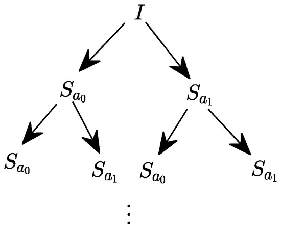
Figure 1. The binary tree structure of the multiple subdivision $S_{{\mathit{a}}_{\mathbf{ϵ}}.}$.

2.2. Iterated Function Systems with Generalizations

Let $(X,d)$ be a complete metric space. For a function $f:X\to X$, let the corresponding Lipschitz constant be defined as

$$Lip\left(f\right)=\underset{x,y\in X,x\ne y}{sup}\frac{d\left(f\right(x),f(y\left)\right)}{d(x,y)}.$$

The function f is said to be contractive if $Lip\left(f\right)<1$. Denote by $\mathbb{H}\left(X\right)$ the collection of all nonvoid compact subsets of X. Then, $\mathbb{H}\left(X\right)$ is a complete metric space endowed with the Hausdorff metric

$$h(B,C)=max\left\{d\right(B,C),d(C,B\left)\right\},$$

where $d(B,C)={sup}_{b\in B}d(b,C)={sup}_{b\in B}{inf}_{c\in C}d(b,c)$ [9].

An iterated function system consists of a finite family of continuous maps $f_i:X\to X$ with $i\in \{1,...,s\}$, which we denote by $\mathcal{F}=\{X;f_i:i=1,..,s\}$. For $\mathcal{F}:\mathbb{H}\left(X\right)\to \mathbb{H}\left(X\right)$

$$\mathcal{F}\left(B\right):={\cup }_{f\in \mathcal{F}}f\left(B\right),B\in \mathbb{H}\left(X\right),$$

where $f\left(B\right):=\left\{f\right(b):b\in B\}$, the Lipschitz constant is $L_{\mathcal{F}}={max}_{i=1,...,s}Lip\left(f_i\right)$. A set A is an attractor of the iterated function system $\mathcal{F}$ if $\mathcal{F}\left(A\right)=A$, which can be generated by the iteration procedure $A_{i+1}=\mathcal{F}\left(A_i\right)$ with an initial set $A_0$.

Schaefer et al. [7] presented the connection between a stationary subdivision $S_{\mathit{a}}$ and fractals and constructed the iterated function systems with

$$f_i\left(X\right)=X{P}^{-1}{S}_{i}P,i=1,\cdots ,s.$$

Here, the $n\times n$ matrix P is constructed with the n points in the following way: the first m columns are the n given control points in ${\mathbb{R}}^m$; the last column is a column of $1^{\prime }s$; the rest columns are such that the matrix P is non-singular while the matrix $S_i$ with the same size as $P^0$ is the subdivision matrix obtained by breaking the matrix S in (2) into multiple $n\times n$ submatrices. In this way, it can be seen that with $X=P$, the corresponding attractor is just the limit of the subdivision scheme [7].

In [9], the authors generalized the above iterated function systems and presented the relationship between fractals and non-stationary subdivision. Now, we cite the following definitions and results.

Definition 1

([9]). The backward trajectory ${\Psi }_k\left(x\right)$ in X starting from $x\in X$ is defined to be

$${\Psi }_k\left(x\right)=T_1\circ T_2\cdots T_k\left(x\right).$$

Theorem 1

([9]). Consider the Function Systems defined by ${\mathcal{F}}_i=\{X;f_{i,1},f_{i,2},\cdots ,f_{i,n_i}\}$, $i\in \Lambda \subset \mathbb{N}$, where $f_{i,r}:X\to X$, $r=1,\cdots ,n_i$, are contractive. Further, assume that $\exists C\subset X$, a compact invariant domain of $\left\{f_{i,r}\right\}$, and assume that, for the Lipschitz constants $L_{{\mathcal{F}}_i}$,

$${\sum }_{k=1}^{\infty }\prod _{i=1}^k{L}_{{\mathcal{F}}_i}<\infty .$$

(3)

Then, the backward trajectories $\left\{{\psi }_k\left(A\right)\right\}$ converge, for any initial set $A\subset C$, to a unique set (attractor) $P\subset C$.

3. Multiple-Function Systems Based on Subdivision

This section is devoted to the construction of the multiple function systems based on regular subdivision. To this end, we construct the corresponding iterated function systems based on subdivision operators and obtain the set of function systems with some necessary modifications.

Building Multiple-Function Systems Based on Regular Subdivision

Let $S_{\mathit{a}}$ be a subdivision with the dilation matrix M. For such a subdivision operator, we can obtain the corresponding iterated function system (see [7]) as

$$\mathcal{F}=\{X;f_1,f_2,\cdots ,f_{\tilde{n}}\},$$

(4)

where $f_i:X\to X$ is a continuous transformation defined as

$$f_i\left(A\right)=A{P}^{-1}{S}_{i}P,A\subset Q^{n-1}.$$

(5)

Here, $Q^{n-1}$ is the $n-1$ dimensional hyperplane with points of the form $(x_1,\cdots ,x_{n-1},1)$, $S_i$ is the ith $n\times n$ subdivision matrix obtained from the subdivision operator $S_{\mathit{a}}$. Note that $P^{-1}{S}_{i}P=\left(\begin{array}{cc}{G}_i& \mathbf{0}\\ b_i& 1\end{array}\right)$, where $f_i:Q^{n-1}\to Q^{n-1}$, thus we actually have

$$f_i\left(A\right)=(\overline{A}{G}_i+b_i,1),A=(\overline{A},1)\subset Q^{n-1}.$$

Now, we build the desired multiple-function systems based on the above iterated function systems. For simplicity, let $S_{{\mathit{a}}_1}$ and $S_{{\mathit{a}}_2}$ denote two subdivision operators. For the subdivision $S_{{\mathit{a}}_1}$ and $S_{{\mathit{a}}_2}$, we choose the same initial points to form the matrix P and obtain the two function systems as follows,

$${\tilde{\mathcal{F}}}^0=\{f_{0,1},\cdots ,f_{0,{\tilde{n}}_0}\},{\tilde{\mathcal{F}}}^1=\{f_{1,1}.\cdots ,f_{1,{\tilde{n}}_1}\}.$$

Then, we make two kinds of modifications to the above iterated function systems: deleting some transformations in one function systems and replacing a transformation in one function system by another transformation in the other one. Then, we can obtain a set of new two function systems as $\{{\mathcal{F}}_0,{\mathcal{F}}_1\}$, where

$${\mathcal{F}}_0=\{f_{0,1},\cdots ,f_{0,n_0}\},{\mathcal{F}}_1=\{f_{1,1},\cdots ,f_{1,n_1}\}.$$

Here, we can also choose ${\mathcal{F}}_0={\tilde{F}}_0$ and ${\mathcal{F}}_1={\tilde{F}}_1$ without modifications. In this way, we can obtain the desired sequence of function system ${\mathcal{F}}_{ϵ}$ as

$${\mathcal{F}}_{ϵ}={\mathcal{F}}_{{ϵ}_1}\circ {\mathcal{F}}_{{ϵ}_2}\circ \cdots {\mathcal{F}}_{{ϵ}_k}\circ \cdots .$$

(6)

with $\mathbf{ϵ}=({ϵ}_1,{ϵ}_2,\cdots )\in {\mathbb{Z}}_2^{\infty }$, which is the desired multiple-function systems.

For such a multiple-function system, in each step of iteration, we choose one function system from $\{{\mathcal{F}}_0,{\mathcal{F}}_1\}$. Therefore, similar to multiple subdivision and the work in [11], we can rewrite ${\mathcal{F}}_{ϵ}$ in a binary tree structure, as shown in Figure 2.

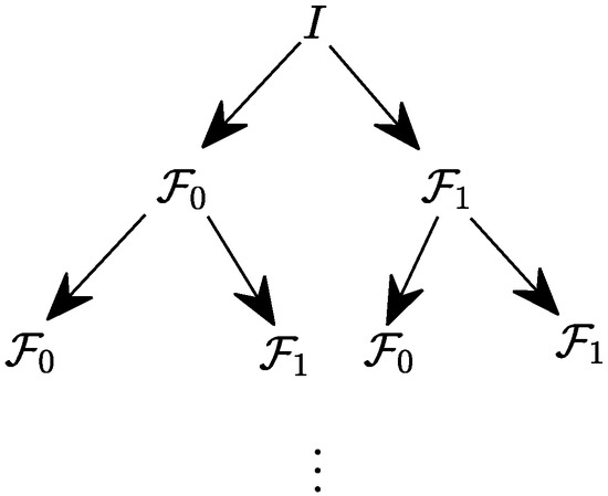
Figure 2. The binary tree structure of the Function Systems ${\mathcal{F}}_{\mathbf{ϵ}}$.

For such a multiple-function system, it can be seen that along the path $P_{ϵ}=({ϵ}_1,{ϵ}_2,\cdots )$ in the above tree structure, we have a map as in (6) with a specific choice of $\mathbf{ϵ}$. Together with the definition of ${\mathcal{F}}_i$, this map along the path $P_{\mathbf{ϵ}}$ can also be written in the tree structure, as shown in Figure 3, where ${ϵ}_p\in \{0,1\}$,

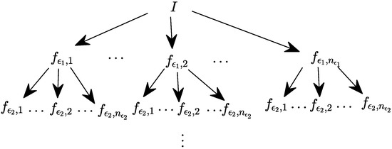
Figure 3. The tree structure of the function system ${\mathcal{F}}_{\mathbf{ϵ}}$ with certain choice of $\mathbf{ϵ}$.

Remark 1.

In fact, the attractor of ${\mathcal{F}}_{\mathbf{ϵ}}$ is the set ${\cup }_{j_1,j_2,\cdots ,j_k,\cdots }{f}_{{ϵ}_1,j_1}\circ f_{{ϵ}_2,j_2}\circ \cdots f_{{ϵ}_k,j_k}\left(A\right)$. When $S_{{\mathit{a}}_1}=S_{{\mathit{a}}_2}$, we only make the modification by deleting some transformations to obtain different function systems. Additionally, we can also get a set of p function systems and arrange the corresponding multiple-function system in a p-ary tree structure.

4. Attractors of the Multiple-Function Systems

Now, we show the convergence of the multiple-function systems. To this purpose, we need to show the convergence along all the paths in the tree structure, which means the convergence of ${\mathcal{F}}_{\mathbf{ϵ}}$ for each choice of $\mathbf{ϵ}$. For this, we first show the following result.

Lemma 1.

Suppose $p^0$ and $p^1$ are two adjacent points in ${\mathbb{R}}^m$. Then, along a path $P_{\mathbf{ϵ}}$ in the tree structure in Figure 3, $f_{{ϵ}_1,j_1}\circ f_{{ϵ}_2,j_2}\circ \cdots \circ f_{{ϵ}_k,k_k}\left(p^0\right)$ and $f_{{ϵ}_1,j_1}\circ f_{{ϵ}_2,j_2}\circ \cdots \circ f_{{ϵ}_k,k_k}\left(p^1\right)$ with ${ϵ}_k\in \{0,1\},j_k\in \{0,\cdots ,n_{{ϵ}_p}\}$ converges to a unique limit point in ${\mathbb{R}}^m$ as k tends to infinity.

Proof. 

From the definition of $f_{{ϵ}_p,j_q}$, the maps along each path in Figure 3 converges. Now, we show the unique limit of the adjacent points.

For the transformation $f_{{ϵ}_p,j_q}$, $f_{{ϵ}_p,j_q}\left(A\right)=(\overline{A}{G}_{{ϵ}_p,j_q}+b_{{ϵ}_p,j_q},1)$, $A=(\overline{A},1)\subset Q^{n-1}$. Therefore, we have

$$\begin{array}{cc}\hfill f_{{ϵ}_1,j_1}\circ f_{{ϵ}_2,j_2}\left(A\right)& =f_{{ϵ}_1,j_1}\left(f_{{ϵ}_2,j_2}\left(A\right)\right)\hfill \\ \hfill & =(\overline{A}{G}_{{ϵ}_2,j_2}+b_{{ϵ}_2,j_2})G_{{ϵ}_1,j_1}+b_{{ϵ}_1,j_1},1)\hfill \\ \hfill & =(\overline{A}{G}_{{ϵ}_2,j_2}{G}_{{ϵ}_1,j_1}+b_{{ϵ}_2,j_2}{G}_{{ϵ}_1,j_1}+b_{{ϵ}_1,j_1},1).\hfill \end{array}$$

Generally, we have

$$\begin{array}{cc}\hfill f_{{ϵ}_1,j_1}\circ \cdots \circ f_{{ϵ}_k,j_k}\left(A\right)& =(\overline{A}{G}_{{ϵ}_k,j_k}\cdots G_{{ϵ}_1,j_1}+b_{{ϵ}_k,j_k}{G}_{{ϵ}_{k-1},j_{k-1}}\cdots G_{{ϵ}_1,j_1}+b_{{ϵ}_{k-1},j_{k-1}}{G}_{{ϵ}_{k-2},j_{k-2}}\cdots G_{{ϵ}_1,j_1}\hfill \\ \hfill & +\cdots +b_{{ϵ}_1,j_1},1).\hfill \end{array}$$

Let $A_1=({\overline{A}}_1,1)$ and $A_2=({\overline{A}}_2,1)$ be the two $n\times n$ matrix made as the matrix P in Section 2.2 using n copies of $p^0$ and $p^1$. In this way, we have

$$\left|\right|f_{{ϵ}_1,j_1}\circ \cdots \circ f_{{ϵ}_k,j_k}\left(A_1\right)-f_{{ϵ}_1,j_1}\circ \cdots \circ f_{{ϵ}_k,j_k}\left(A_2\right)\left|\right|\le \left|\right|{\overline{A}}_1-{\overline{A}}_2\left|\right|\left|\right|G_{{ϵ}_1,j_1}\left|\right|\cdots \left|\right|G_{{ϵ}_k,j_k}\left|\right|.$$

According to the eigenvalues of the subdivision matrix, the eigenvalues of $G_{{ϵ}_p,j_q}$ are smaller than 1, we have

$$\underset{k\to \infty }{lim}\left|\right|f_{{ϵ}_k,j_k}\circ \cdots \circ f_{{ϵ}_1,j_1}\left(A_1\right)-f_{{ϵ}_k,j_k}\circ \cdots \circ f_{{ϵ}_1,j_1}\left(A_2\right)\left|\right|\le \underset{k\to \infty }{lim}\left|\right|G_{{ϵ}_1,j_1}\left|\right|\cdots \left|\right|G_{{ϵ}_k,j_k}\left|\right|\left|\right|{\overline{A}}_1-{\overline{A}}_2\left|\right|=0.$$

This means that $f_{{ϵ}_k,j_k}\circ \cdots \circ f_{{ϵ}_1,j_1}\left(A_1\right)$ and $f_{{ϵ}_k,j_k}\circ \cdots \circ f_{{ϵ}_1,j_1}\left(A_2\right)$ converge to the same limit point. □

Remark 2.

The matrix $A_0$ and $A_1$ here need not be invertible. Furthermore, by Lemma 1, for the matrix P composed of n different points, the corresponding limit is a vector of n identical points in ${\mathbb{R}}^m$, which can also be verified following Remark $6.2$ in [9].

Theorem 2.

Let $S_{{\mathit{a}}_1}$ and $S_{{\mathit{a}}_2}$ be two convergent subdivision and ${\mathcal{F}}_{\mathbf{ϵ}}$ with $ϵ=({ϵ}_1,\cdots )$, ${ϵ}_j\in \{0,1\}$ be the multiple-function system obtained based on $S_{{\mathit{a}}_1}$ and $S_{{\mathit{a}}_2}$. Then, for each ϵ, the trajectory ${\mathcal{F}}_{{ϵ}_1}\circ \cdots {\mathcal{F}}_{{ϵ}_k}\left(A\right)$ with $A\subset Q^{n-1}$ converges to a unique attractor.

Proof. 

Let $\left\{L_{{\mathcal{F}}_i}\right\}$ be the corresponding contractive factors of the obtained function systems ${\mathcal{F}}_i$ with $i=0,1$. For the k steps of iterations, if there are p steps of iterations using ${\mathcal{F}}_1$, there are $k-t$ steps of iterations using ${\mathcal{F}}_0$. Then, from the construction of the function systems ${\mathcal{F}}_0$ and ${\mathcal{F}}_1$, we have

$$\prod _{i=1}^k{L}_{{\mathcal{F}}_i}=L_{{\mathcal{F}}_0}^{k-t}{L}_{{\mathcal{F}}_1}^t.$$

Since $S_i$ converges, $L_{{\mathcal{F}}_i}<1$, thus,

$$\sum _{k=1}^{\infty }\prod _{i=1}^k{L}_{{\mathcal{F}}_i}\le \sum _{k=1}^{\infty }{L}_{{\mathcal{F}}_0}^{k-t}{L}_{{\mathcal{F}}_1}^t<\infty .$$

Therefore, by Theorem 1, the backward trajectory $\left\{{\Psi }_k\left(A\right)\right\}$ converges.

By Remark 2, starting the backward trajectory $\left\{{\Psi }_k\left(A\right)\right\}$ initialized with $A\subset Q^{n-1}$ converges to a vector of n equal points in ${\mathbb{R}}^m$. Then, similar to the proof of Theorem $7.2$ in [9], we can show that the trajectory converges to the same limit for any $A\subset Q^{n-1}$. □

Theorem 2 shows the convergence of a multiple-function system along a certain path. Therefore, along different paths, the convergence can be shown and different attractors can be obtained. Thus, the obtained attractor generated by the multiple-function system is path-dependent. Moreover, since the attractor generated by a multiple-function system is path-dependent, the corresponding dimension is also path-dependent. This can be shown by the examples in Section 5.

5. Numerical Examples

This section is devoted to several numerical examples of the new multiple-function systems. These numerical examples show the multiple-function systems can generate different attractors along different paths.

Example 1.

The ternary D-D 2-pt subdivision can be characterized by the symbol $a\left(z\right)=z^{-2}\frac{{(1+z+z^2)}^2}{3}$. We choose the two points 0 and 1 in the x-axis, thus, we have the matrix P as follows,

$$P=\left(\begin{array}{cc}0& 1\\ 1& 1\end{array}\right).$$

The subdivision matrices we need are the following

$$S_1=\left(\begin{array}{cc}1& 0\\ \frac{2}{3}& \frac{1}{3}\end{array}\right),S_2=\left(\begin{array}{cc}\frac{2}{3}& \frac{1}{3}\\ \frac{1}{3}& \frac{2}{3}\end{array}\right),S_3=\left(\begin{array}{cc}\frac{1}{3}& \frac{2}{3}\\ 0& 1\end{array}\right).$$

In this way, we have the function system ${\mathcal{F}}_0=\{f_{0,1},f_{0,2},f_{0,3}\}$, with

$$f_{0,i}\left(A\right)=A{P}^{-1}{S}_{i}P,i=1,2,3.$$

Now, based on ${\mathcal{F}}_0$, we give the second function system as ${\mathcal{F}}_1=\{f_{1,1},f_{1,2}\}$ with $f_{1,1}=f_{0,1}$, $f_{1,2}=f_{0,3}$. Therefore, we have the multiple-function system

$${\mathcal{F}}_{\mathbf{ϵ}}^1={\mathcal{F}}_{{ϵ}_1}\circ {\mathcal{F}}_{{ϵ}_2}\circ \cdots ,$$

with $ϵ=({ϵ}_1,\cdots ,{ϵ}_k,\cdots )$ and ${ϵ}_i\in \{0,1\}$.

Figure 4 shows the attractors generated by this multiple-function system ${\mathcal{F}}_{\mathbf{ϵ}}^1$ with different choices of $\mathbf{ϵ}$. In particular, when $ϵ=(0,0,\cdots )$, the obtained attractor is a line and when $ϵ=(1,1,\cdots )$ the obtained attractor is actually the Cantor set. Furthermore, the dimension of the attractor along the path $(0,0,\cdots )$ is $d=1$ and the dimension of the Cantor set along the path $(1,1,\cdots )$ is $d={log}_{3}2$.

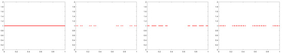
Figure 4. Attractors generated by the multiple-function system ${\mathcal{F}}_{\mathbf{ϵ}}^1$ with $ϵ=(0,0,0,0,0)$, $(1,1,1,1,1),(1,0,1,0,1),(0,1,0,1,0)$ (from left to right).

Example 2.

Now, we give the scheme of the tensor product of the ternary D-D 2-pt scheme. In fact, such a scheme can be characterized by the symbol $a(z_1,z_2)=z_1^{-2}{z}_2^{-2}\frac{{(1+z_1+z_1^2)}^2{(1+z_2+z_2^2)}^2}{9}$.

Here, we choose the four points $(0,0,0),(1,0,0),(0,1,0),(1,1,2)$ to derive the matrix P as

$$P=\left(\begin{array}{cccc}0& 0& 0& 1\\ 1& 0& 0& 1\\ 0& 1& 0& 1\\ 1& 1& 2& 1\end{array}\right).$$

The corresponding subdivision matrices we need to obtain the contractive maps are as follows,

$$\begin{array}{cc}\hfill & S_1=\left(\begin{array}{cccc}1& 0& 0& 0\\ \frac{2}{3}& \frac{1}{3}& 0& 0\\ \frac{2}{3}& 0& \frac{1}{3}& 0\\ \frac{4}{9}& \frac{2}{9}& \frac{2}{9}& \frac{1}{9}\end{array}\right),S_2=\left(\begin{array}{cccc}\frac{2}{3}& \frac{1}{3}& 0& 0\\ \frac{1}{3}& \frac{2}{3}& 0& 0\\ \frac{4}{9}& \frac{2}{9}& \frac{2}{9}& \frac{1}{9}\\ \frac{2}{9}& \frac{4}{9}& \frac{1}{9}& \frac{2}{9}\end{array}\right),S_3=\left(\begin{array}{cccc}\frac{1}{3}& \frac{2}{3}& 0& 0\\ 0& 1& 0& 0\\ \frac{2}{9}& \frac{4}{9}& \frac{1}{9}& \frac{2}{9}\\ 0& \frac{2}{3}& 0& \frac{1}{3}\end{array}\right),\hfill \\ \hfill & S_4=\left(\begin{array}{cccc}\frac{2}{3}& 0& \frac{1}{3}& 0\\ \frac{4}{9}& \frac{2}{9}& \frac{2}{9}& \frac{1}{9}\\ \frac{1}{3}& 0& \frac{2}{3}& 0\\ \frac{2}{9}& \frac{1}{9}& \frac{4}{9}& \frac{2}{9}\end{array}\right),S_5=\left(\begin{array}{cccc}\frac{4}{9}& \frac{2}{9}& \frac{2}{9}& \frac{1}{9}\\ \frac{2}{9}& \frac{4}{9}& \frac{1}{9}& \frac{2}{9}\\ \frac{2}{9}& \frac{1}{9}& \frac{4}{9}& \frac{2}{9}\\ \frac{1}{9}& \frac{2}{9}& \frac{2}{9}& \frac{4}{9}\end{array}\right),S_6=\left(\begin{array}{cccc}\frac{2}{9}& \frac{4}{9}& \frac{1}{9}& \frac{2}{9}\\ 0& \frac{2}{3}& 0& \frac{1}{3}\\ \frac{1}{9}& \frac{2}{9}& \frac{2}{9}& \frac{4}{9}\\ 0& \frac{1}{3}& 0& \frac{2}{3}\end{array}\right),\hfill \end{array}$$

$$\begin{array}{cc}\hfill & S_7=\left(\begin{array}{cccc}\frac{1}{3}& 0& \frac{2}{3}& 0\\ \frac{2}{9}& \frac{1}{9}& \frac{4}{9}& \frac{2}{9}\\ 0& 0& 1& 0\\ 0& 0& \frac{2}{3}& \frac{1}{3}\end{array}\right),S_8=\left(\begin{array}{cccc}\frac{2}{9}& \frac{1}{9}& \frac{4}{9}& \frac{2}{9}\\ \frac{1}{9}& \frac{2}{9}& \frac{2}{9}& \frac{4}{9}\\ 0& 0& \frac{2}{3}& \frac{1}{3}\\ 0& 0& \frac{1}{3}& \frac{2}{3}\end{array}\right),S_9=\left(\begin{array}{cccc}\frac{1}{9}& \frac{2}{9}& \frac{2}{9}& \frac{4}{9}\\ 0& \frac{1}{3}& 0& \frac{2}{3}\\ 0& 0& \frac{1}{3}& \frac{2}{3}\\ 0& 0& 0& 1\end{array}\right).\hfill \end{array}$$

In this way, we can give the function system ${\mathcal{F}}_0=\{f_{0,1},\cdots ,f_{0,9}\}$ with $f_{0,i}\left(A\right)=A{P}^{-1}{S}_{i}P$, $i=1,\cdots ,9$. Based on ${\mathcal{F}}_0$, we give the function system ${\mathcal{F}}_1$ as ${\mathcal{F}}_1=\{f_{1,1},\cdots ,f_{1,8}\}$ with $f_{1,i}=f_{0,i}$, $i=1,\cdots ,4$, $f_{1,i}=f_{0,i+1}$, $i=5,\cdots ,8$. In this way, we can derive the multiple-function system ${\mathcal{F}}_{\mathbf{ϵ}}^2$ with the set of function systems $\{{\mathcal{F}}_0,{\mathcal{F}}_1\}$.

Figure 5 shows the attractors generated by this multiple-function system ${\mathcal{F}}_{\mathbf{ϵ}}^2$ with different choice of $\mathbf{ϵ}$. In paticular, when $ϵ=(1,1,\cdots )$, the obtained attractor is actually the Sierpinski garsket. Additionally, the dimension of the attractor obtained along the path $(0,0,\cdots )$ is $d=2$ and the dimension of the attractor obtained along the path $(1,1,\cdots )$ is $d={log}_{3}8$.

Figure 5. Attractors generated by the multiple-function system ${\mathcal{F}}_{ϵ}^2$ with $ϵ=(0,0,0,0)$, $(1,1,1,1),(0,1,1,1),(0,1,0,1),(1,0,1,0),(0,0,0,1)$ (from left to right and top to bottom).

Example 3.

The above two examples are obtained based on a single subdivision. Now, we give an example of a multiple-function system based on different subdivision.

In fact, for the first function system ${\mathcal{F}}_0$, we choose the binary cubic B-spline scheme. We choose the points $(0,0),(\frac{1}{3},0),(\frac{1}{2},\frac{\sqrt{3}}{6}),(\frac{2}{3},0),(1,0)$ and thus, the corresponding matrix P can be written as

$$P=\left(\begin{array}{ccccc}0& 0& 1& 0& 1\\ \frac{1}{3}& 0& 0& 1& 1\\ \frac{1}{2}& \frac{\sqrt{3}}{6}& 0& 0& 1\\ \frac{2}{3}& 0& 0& 0& 1\\ 1& 0& 0& 0& 1\end{array}\right).$$

The subdivision matrices we need are as follows,

$$S_{0,1}=\left(\begin{array}{ccccc}\frac{1}{2}& \frac{1}{2}& 0& 0& 0\\ \frac{1}{8}& \frac{3}{4}& \frac{1}{8}& 0& 0\\ 0& \frac{1}{2}& \frac{1}{2}& 0& 0\\ 0& \frac{1}{8}& \frac{3}{4}& \frac{1}{8}& 0\\ 0& 0& \frac{1}{2}& \frac{1}{2}& 0\end{array}\right),S_{0,2}=\left(\begin{array}{ccccc}0& \frac{1}{2}& \frac{1}{2}& 0& 0\\ 0& \frac{1}{8}& \frac{3}{4}& \frac{1}{8}& 0\\ 0& 0& \frac{1}{2}& \frac{1}{2}& 0\\ 0& 0& \frac{1}{8}& \frac{3}{4}& \frac{1}{8}\\ 0& 0& 0& \frac{1}{2}& \frac{1}{2}\end{array}\right),$$

and thus, the corresponding two maps are

$$f_{0,1}\left(A\right)=A{P}^{-1}{S}_{0,1}P,f_{0,2}\left(A\right)=A{P}^{-1}{S}_{0,2}P,$$

and we obtain the function system ${\mathcal{F}}_0=\{f_{0,1},f_{0,2}\}$. As for the second one, we keep the matrix P and choose the subdivision for the Koch curve with the following subdivision matrices,

$$\begin{array}{cc}\hfill & S_{1,1}=\left(\begin{array}{ccccc}1& 0& 0& 0& 0\\ \frac{2}{3}& \frac{1}{3}& 0& 0& 0\\ \frac{2}{3}& 0& \frac{1}{3}& 0& 0\\ \frac{1}{3}& \frac{2}{3}& 0& 0& 0\\ 0& 1& 0& 0& 0\end{array}\right),S_{1,2}=\left(\begin{array}{ccccc}0& 1& 0& 0& 0\\ 0& \frac{2}{3}& \frac{1}{3}& 0& 0\\ \frac{1}{3}& 0& \frac{2}{3}& 0& 0\\ 0& \frac{1}{3}& \frac{2}{3}& 0& 0\\ 0& 0& 1& 0& 0\end{array}\right),\hfill \\ \hfill & S_{1,3}=\left(\begin{array}{ccccc}0& 0& 1& 0& 0\\ 0& 0& \frac{2}{3}& \frac{1}{3}& 0\\ 0& 0& \frac{2}{3}& 0& \frac{1}{3}\\ 0& 0& \frac{1}{3}& \frac{2}{3}& 0\\ 0& 0& 0& 1& 0\end{array}\right),S_{1,4}=\left(\begin{array}{ccccc}0& 0& 0& 1& 0\\ 0& 0& 0& \frac{2}{3}& \frac{1}{3}\\ 0& 0& \frac{1}{3}& 0& \frac{2}{3}\\ 0& 0& 0& \frac{1}{3}& \frac{2}{3}\\ 0& 0& 0& 0& 1\end{array}\right),\hfill \end{array}$$

and the corresponding maps are

$$f_{1,i}\left(A\right)=A{P}^{-1}{S}_{1,i}P,i=1,\cdots ,4,$$

and thus, we have the function system ${\mathcal{F}}_1=\{f_{1,i},i=1,\cdots ,4\}$.

In this way, we can obtain the multiple-function system ${\mathcal{F}}_{\mathbf{ϵ}}^3$. Figure 6 shows the attractors generated by this multiple-function system with different choice of $\mathbf{ϵ}$.

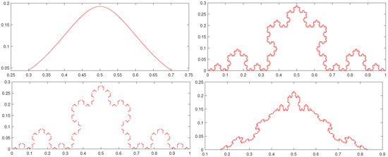
Figure 6. Attractors generated by the multiple-function system ${\mathcal{F}}_{\mathbf{ϵ}}^3$ with $\mathbf{ϵ}=(0,0,0,0,0)$, $(1,1,1,1,1),(1,0,1,1,1),(1,1,1,1,0)$ (from left to right and top to bottom).

6. Conclusions

This paper presents the multiple-function systems based on regular subdivision operators. The multiple-function systems introduced in this paper have a set of function systems and choose one for each step of iteration. Thus, a multiple-function system ${\mathcal{F}}_{\mathbf{ϵ}}$ can generate different attractors with different choices of $\mathbf{ϵ}$. Such multiple-function systems can be seen as being obtained by making some necessary modifications to the iteration function systems based on subdivision operators. For such multiple-function systems, we show that they can be arranged in a tree structure and show the existence and uniqueness of the attractor along each path in the tree structure. Although the new multiple-function systems can generate different attractors, they cannot design certain fractal at certain position. Therefore, in future work, we hope to design different transformations like location dependent ones and obtain new multiple-function systems to control the attractor locally and design certain fractal at certain position. Additionally, we hope to exploit the applications of the multiple-function systems in fields such as data compression.

References

- Barnsley, M. Fractals Everywhere; Academic Press: Cambridge, MA, USA, 1993. [Google Scholar]
- Zhang, B.; Zheng, H. A variant exponential B-spline scheme with shape control. Mathematics 2021, 9, 3116. [Google Scholar] [CrossRef]
- Qi, W.; Luo, Z.; Fan, X. Subdivision schemes induced by approximating schemes. Sci. Sin. Math. 2014, 44, 755–768. (In Chinese) [Google Scholar] [CrossRef]
- Sauer, T. Shearlet Multiresolution and Multiple Refinement. In Shearlets; Kutyniok, G., Labate, D., Eds.; Springer: Berlin/Heidelberg, Germany, 2011. [Google Scholar]
- Kutyniok, G.; Sauer, T. Adaptive directional subdivision schemes and shearlet multiresolution analysis. Siam J. Math. Anal. 2009, 41, 1436–1471. [Google Scholar] [CrossRef]
- Novara, P.; Romani, L.; Yoon, J. Improving smoothness and accuracy of Modified Butterfly subdivision scheme. Appl. Math. Comput. 2016, 272, 64–79. [Google Scholar] [CrossRef]
- Schaefer, S.; Levin, D.; Goldman, R. Subdivision schemes and attractors. In Proceedings of the Third Eurographics Symposium on Geometry Processing, Vienna, Austria, 4–6 July 2005. [Google Scholar]
- Prautzsch, H.; Micchelli, C. Computing curves in variant under halving. Comput. Aided Geom. Des. 1987, 4, 133–140. [Google Scholar] [CrossRef]
- Levin, D.; Dyn, N.; Veedu, V.P. Non-stationary versions of fixed-point theory, with applications to fractals and subdivision. J. Fixed Point Theory Appl. 2019, 21, 26. [Google Scholar] [CrossRef]
- Hu, Y.; Zheng, H.; Geng, J. Calculation of dimensions of curves generated by subdivision schemes. Int. J. Comput. Math. 2019, 96, 1278–1291. [Google Scholar] [CrossRef]
- Dyn, N.; Levin, D.; Massopust, P. Attractors of trees of maps and of sequences of maps between spaces with applications to subdivision. J. Fixed Point Theory Appl. 2020, 22, 14. [Google Scholar] [CrossRef]
- Barlow, M.; Hambly, B. Transition density estimates for Brownian motion on scale irregular Sierpinski gaskets. Ann. I’Institut Henri Poincare(B) Probab. Stat. 1997, 33, 531–557. [Google Scholar] [CrossRef]
Publisher’s Note: MDPI stays neutral with regard to jurisdictional claims in published maps and institutional affiliations. |
© 2022 by the authors. Licensee MDPI, Basel, Switzerland. This article is an open access article distributed under the terms and conditions of the Creative Commons Attribution (CC BY) license (https://creativecommons.org/licenses/by/4.0/).