Maximum Likelihood Estimation for Mixed Fractional Vasicek Processes

Abstract

In this paper, we consider the problem of estimating the drift parameters in the mixed fractional Vasicek model, which is an extended model of the traditional Vasicek model. Using the fundamental martingale and the Laplace transform, both the strong consistency and the asymptotic normality of the maximum likelihood estimators are studied for all $H\in (0,1)$, $H\ne 1/2$. On the other hand, we present that the MLE can be simulated when the Hurst parameter $H>1/2$.

1. Introduction

The standard Vasicek models, including the diffusion models based on Brownian motion and the jump-diffusion models driven by Lévy processes, provide good service in cases where the data demonstrate the Markovian property and a lack of memory. However, over the past few decades, numerous empirical studies have found that the phenomenon of long-range dependence may be observed in the data of hydrology, geophysics, climatology, telecommunication, economics, and finance. Consequently, several time series models or stochastic processes have been proposed to capture long-range dependence, both in discrete time and in continuous time. In the continuous time case, the best-known and widely used stochastic process that exhibits long-range dependence or short-range dependence is of course the fractional Brownian motion (fBm), which describes the degree of dependence by the Hurst parameter. This naturally explains the appearance of fBm in the modeling of some properties of “real-world” data. As well as in the diffusion model with the fBm, the mean-reverting property is very attractive to understand volatility modeling in finance. Hence, the fractional Vasicek model (fVm) becomes the usual candidate to capture some phenomena of the volatility of financial assets (see, for example, [1,2,3]). More precisely, the fVm can be described by the following Langevin equation:

$$d{X}_t=\left(\alpha -\beta X_t\right)dt+\gamma d{B}_t^H,t\in [0,T],$$

(1)

where $\beta ,\gamma \in {\mathbb{R}}^{+}$, $\alpha \in \mathbb{R}$, the initial condition is set at $X_0=0$, and $B_t^H$, an fBm with Hurst parameter $H\in (0,1)$, is a zero mean Gaussian process with the covariance:

$$\mathbb{E}\left(B_t^H{B}_s^H\right)=R_H(s,t)=\frac{1}{2}\left({\left|t\right|}^{2H}+{\left|s\right|}^{2H}-{|t-s|}^{2H}\right).$$

(2)

The process $B_t^H$ is self-similar in the sense that $\forall a\in R^{+}$, $B_{at}^H\stackrel{d}{=}{a}^H{B}_t^H$. It becomes the standard Brownian motion $W_t$ when $H=1/2$ and can be represented as a stochastic integral with respect to the standard Brownian motion. When $1/2<H<1$, it has long-range dependence in the sense that ${\sum }_{n=1}^{\infty }\mathbb{E}\left(B_1^H(B_{n+1}^H-B_n^H)\right)=\infty$. In this case, the positive (negative) increments are likely to be followed by positive (negative) increments. The parameter H, which is also called the self-similarity parameter, measures the intensity of the long-range dependence. Recently, borrowing the idea of [4], these papers [5,6] used the mixed fractional Vasicek model (mfVm) to describe some phenomena of the volatility of financial assets, which can be expressed as:

$$d{X}_t=(\alpha -\beta X_t)dt+\gamma d{\xi }_t,t\in [0,T],X_0=0.$$

(3)

where $\beta ,\gamma \in {\mathbb{R}}^{+}$, $\alpha \in \mathbb{R}$, and the initial condition is set at $X_0=0$. Here, the process of the so-called mixed fractional Brownian motion $\xi =({\xi }_t,t\in [0,T])$ is defined by ${\xi }_t=W_t+B_t^H,$$H\in (0,1)$ where W and $B^H$ are independent standard and fractional Brownian motions.

When the long-term mean $\alpha$ in (3) is known (without loss of generality, it is assumed to be zero), (3) becomes the mixed fractional Ornstein–Uhlenbeck process (mfOUp). Using the canonical representation and spectral structure of the mfBm, the authors of [7] originally proposed the maximum likelihood estimator (MLE) of $\beta$ in (3) and considered the asymptotical theory for this estimator with the Laplace transform and the limit presence of the eigenvalues of the covariance operator for the fBm (see [8]). Using an asymptotic approximation for the eigenvalues of its covariance operator, the paper of [9] explained the mfBm from the viewpoint of spectral theory. Some surveys and a complete literature related to the parametric and other inference procedures for stochastic models driven by the mfBm were summarized in a recent monograph of [10,11].

However, in some situations, the long-term mean $\alpha$ in (3) is always unknown. Thus, it is important to estimate all the drift parameters, $\alpha$ and $\beta$, in the mfVm. To the best of our knowledge, the asymptotic theory of the MLE of $\alpha$ and $\beta$ has not developed yet; even some methods for the fractional diffusion cases can be applied in this situation (e.g., see [12]). This paper fills in the gaps in this area. Using the Girsanov formula for the mfBm, we introduce the MLE for both $\alpha$ and $\beta$. When a continuous record of observations of $X_t$ is available, both the strong consistency and the asymptotic laws of the MLE are established in the stationary case for the Hurst parameter $H\in (0,1)$.

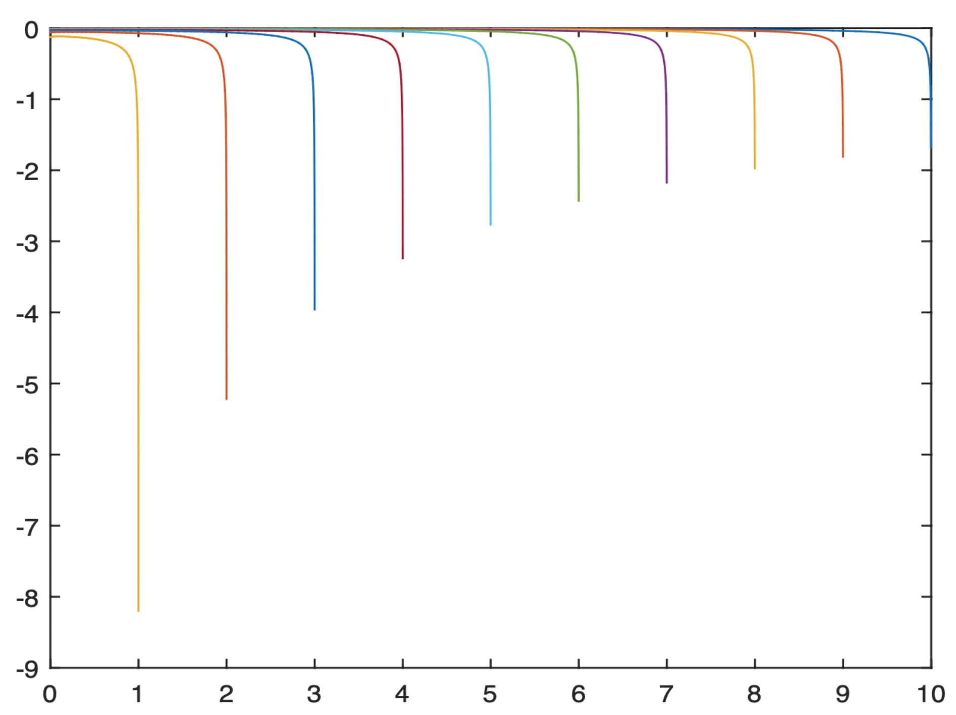
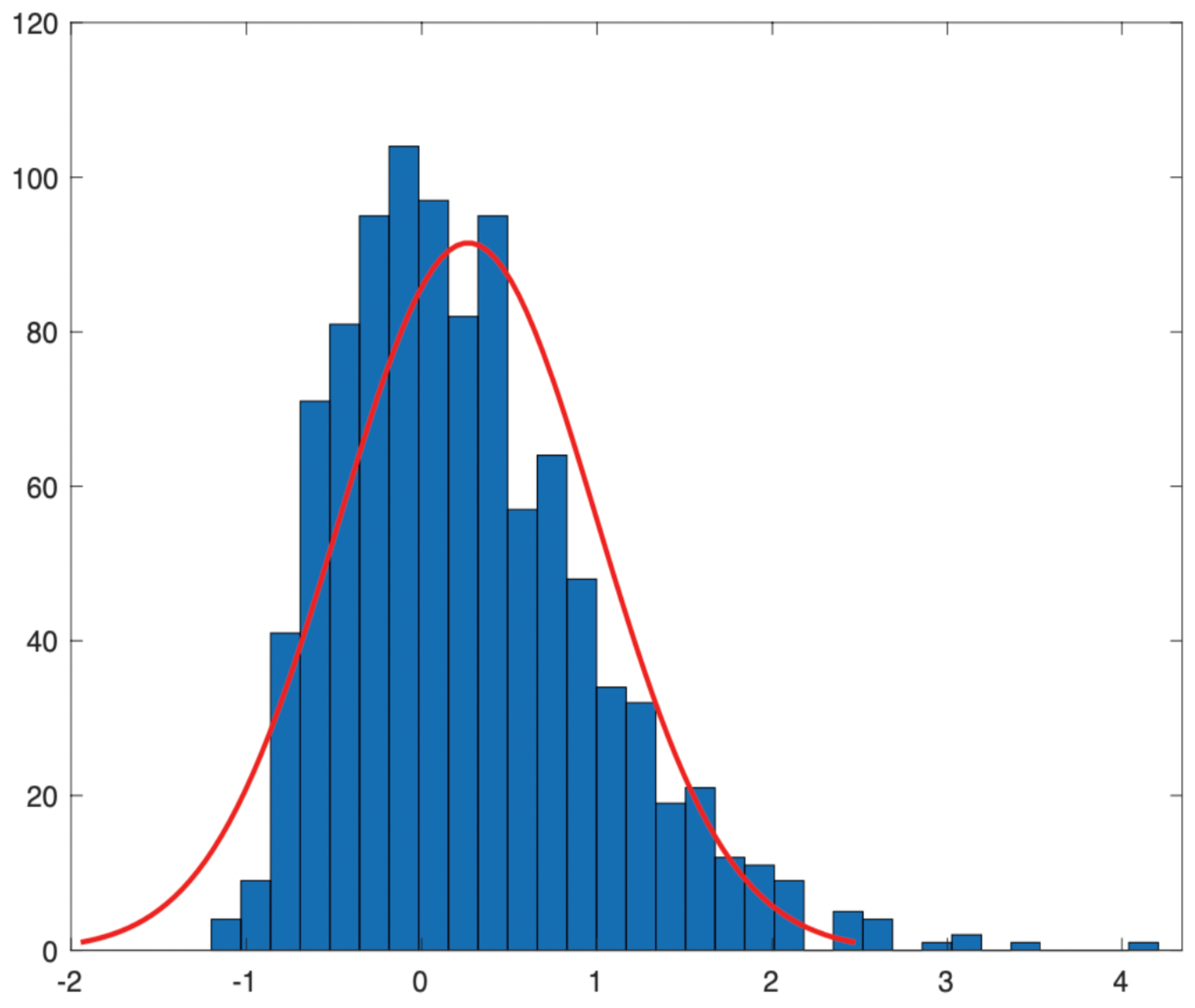
In the aspect of simulation, as far as we know, until now, there are few works referring to the exact experiment for the MLE even in the fractional O-U process. The difficulties come from the process $Q_t$ defined in (9): it is not easy to simulate and also will cost much time. Here, we try to illustrate that the MLE of the drift parameter in the mixed fractional O-U process (the same for the Vasicek process) can be achieved when $H>1/2$, even if it is not practical.

The rest of the paper is organized as follows. Section 2 introduces some preliminaries of the mfBm. Section 3 proposes the MLE for the drift parameters in the mfVm and studies the asymptotic properties of the MLE for the Hurst parameter range $H\in (0,1)$ in the stationary case. Section 4 provides the proofs of the main results of this paper. We complete with the simulation of the drift parameter in Section 5. Some technical lemmas are gathered in Section 6. We use the following notations throughout the paper: $\stackrel{a.s.}{\to }$, $\stackrel{\mathbf{P}}{\to }$, $\stackrel{d}{\to }$, and ∼ denote convergence almost surely, convergence in probability, convergence in distribution, and asymptotic equivalence, respectively, as $T\to \infty$.

2. Preliminaries

This section is dedicated to some notions that are used in our paper, related mainly to the integro-differential equation and the Radon–Nikodym derivative of the mfBm. In fact, mixtures of stochastic processes can have properties quite different from the individual components. The mfBm drew considerable attention since some of its properties were discovered in [4,11,13]. Moreover, the mfBm has been proven useful in mathematical finance (see, for example, [14]). We start by recalling the definition of the main process of our work, which is the mfBm. For more details about this process and its properties, the interested reader can refer to [4,11,13].

Definition 1.

An mfBm of the Hurst parameter $H\in (0,1)$ is a process $\xi =({\xi }_t,t\in [0,T])$ defined on a probability space $(\mathsf{\Omega },\mathcal{F},\mathbf{P})$ by:

$${\xi }_t=W_t+B_t^H,$$

where $W=(W_t,t\in [0,T])$ is the standard Brownian motion and $B^H=(B_t^H,t\in [0,T])$ is the independent fBm with the Hurst exponent $H\in (0,1)$ and the covariance function:

$$K(s,t)=\mathbf{E}{B}_t^H{B}_s^H=\frac{1}{2}\left(t^{2H}+s^{2H}-{|t-s|}^{2H-1}\right).$$

Let us observe that the increments of the mfBm are stationary and ${\xi }_t$ is a centered Gaussian process with the covariance function:

$$\mathbf{E}\left[{\xi }_t^H{\xi }_s^H\right]=min\{t,s\}+\frac{1}{2}\left[t^{2H}+s^{2H}-{|t-s|}^{2H}\right],s,t⩾0.$$

In particular, for $H>1/2$, the increments of the mfBm exhibit long-range dependence, which makes it important in modeling volatility in finance. Let ${\mathcal{F}}^{\xi }=({\mathcal{F}}_t^{\xi },t\in [0,T])$. We use the canonical representation suggested in [13], based on the martingale:

$$M_t=\mathbf{E}\left(W_t\right|{\mathcal{F}}_t^{\xi }),t\in [0,T].$$

(4)

To this end, let us consider the integro-differential equation:

$$g(s,t)+H\frac{d}{ds}{\int }_0^{t}g(r,t){|r-s|}^{2H-1}\mathrm{sign}(s-r)dr=1,0<s\ne t\le T.$$

(5)

By Theorem 5.1 in [13], this equation has a unique solution for any $H\in (0,1)$. It is continuous on $[0,T]$, and the ${\mathcal{F}}^{\xi }$-martingale defined in (4) and its quadratic variation ${\langle M\rangle }_t,t\in [0,T]$ satisfy:

$$M_t={\int }_0^{t}g(s,t)d{\xi }_s,{\langle M\rangle }_t={\int }_0^{t}g(s,t)ds,t\ge 0,t\in [0,T],$$

(6)

where the stochastic integral is defined for $L^2(0,T)$ deterministic integrands in the usual way. By Corollary 2.9 in [13], the process $\xi$ admits canonical representation:

$${\xi }_t={\int }_0^{t}G(s,t)d{M}_s,t\in [0,T]$$

(7)

with:

$$G(s,t)=1-\frac{d}{d{\langle M\rangle }_s}{\int }_0^{t}g(r,s)dr.$$

(8)

Remark 1.

For $H>1/2$, the equation $g(s,t)$ is a Wiener–Höpfner equation:

$$g(s,t)+H(2H-1){\int }_0^{t}g(r,t){|r-s|}^{2H-2}dr=1,0\le s\le t\le T,$$

and the quadratic variation $\langle M\rangle$ is:

$${\langle M\rangle }_t={\int }_0^t{g}^2(s,s)ds$$

Let us mention that the canonical representation (6) and (7) can be also used to derive an analogue of Girsanov’s theorem, which will be the key tool for constructing the MLE.

Corollary 1.

Consider a process $Y=(Y_t,t\in [0,T])$ defined by:

$$Y_t={\int }_0^{t}f\left(s\right)ds+{\xi }_t,t\in [0,T],$$

where $f=\left(f\right(t),t\in [0,T\left]\right)$ is a process with a continuous path and $\mathbf{E}{\int }_0^T\left|f\left(t\right)\right|dt<\infty$, adapted to a filtration $\mathcal{G}=\left({\mathcal{G}}_t\right)$ with respect to a martingale M. Then, Y admits the following representation:

$$Y_t={\int }_0^{t}G(s,t)d{Z}_s$$

with $G(s,t)$ defined in (8), and the process $Z=(Z_t,t\in [0,T])$ can be written as:

$$Z_t={\int }_0^{t}g(s,t)d{Y}_s,t\in [0,T].$$

Let us mention that $Z_t$ is a $\mathcal{G}$-martingale with the Doob–Meyer decomposition:

$$Z_t=M_t+{\int }_0^t\Phi \left(s\right)d{\langle M\rangle }_s,$$

where:

$$\Phi \left(t\right)=\frac{d}{d{\langle M\rangle }_t}{\int }_0^{t}g(s,t)f\left(s\right)ds.$$

In particular, ${\mathcal{F}}_t^Y={\mathcal{F}}_t^Z,\mathbf{P}-a.s.$ for all $t\in [0,T]$. Moreover, if:

$$\mathbf{E}exp\left\{-{\int }_0^T\Phi \left(t\right)d{M}_t-\frac{1}{2}{\int }_0^T{\Phi }^2\left(t\right)d{\langle M\rangle }_t\right\}=1,$$

then the measures ${\mu }^{\xi }$ and ${\mu }^Y$ are equivalent and the corresponding Radon–Nikodym derivative is given by:

$$\frac{d{\mu }^Y}{d{\mu }^{\xi }}\left(Y\right)=exp\left\{{\int }_0^T\widehat{\Phi }\left(t\right)d{Z}_t-\frac{1}{2}{\int }_0^T{\widehat{\Phi }}^2\left(t\right)d{\langle M\rangle }_t\right\},$$

where $\widehat{\Phi }\left(t\right)=\mathbf{E}(\Phi \left(t\right)|{\mathcal{F}}_t^Y)$.

3. Estimators and Asymptotic Behaviors

Now, we return to the model (3); similar to the previous corollary, we define:

$$Z_t={\int }_0^{t}g(s,t)d{X}_s,Q_t=\frac{d}{d{\langle M\rangle }_t}{\int }_0^{t}g(s,t)X_{s}ds,t\in [0,T].$$

(9)

From the following Lemma 10 and Equation (44), we know:

$$Q_t=\frac{\alpha }{\beta }-\frac{\alpha }{\beta }\frac{d}{d{\langle M\rangle }_t}{\int }_0^{t}g(s,t)e^{-\beta s}ds+Q_t^U,$$

where $Q_t^U$ is $Q_t$ when $\alpha =0$. By Theorem 2.4 of [13] and Lemma 2.1 of [7], we know the derivative of the martingale bracket $d{\langle M\rangle }_t/dt$ exists and is continuous, as well as the process $Q_t^U$ admits the representation as the stochastic integral with respect to auxiliary observation process $Z_t$. That is to say, the process $Q_t$ is well defined.

Then, using the quadratic variation of Z on [0, T], we can estimate $\gamma$ almost surely from any small interval as long as we have a continuous observation of the process. Moreover, the estimation of H in the mfBm was performed in [15]. As a consequence, for further statistical analysis, we assumed that H and $\gamma$ are known, and without loss of generality, from now on, we suppose that $\gamma$ is equal to one. For $\gamma =1$, our observation will be $Z=(Z_t,t\in [0,T])$, where $Z_t$ satisfies the following equation:

$$d{Z}_t=(\alpha -\beta Q_t)d{\langle M\rangle }_t+d{M}_t,t\in [0,T].$$

(10)

Applying the analog of the Girsanov formula for an mfBm, we can obtain the following likelihood ratio and the explicit expression of the likelihood function:

$${\mathcal{L}}_T(\alpha ,\beta ,Z^T)=exp\left({\int }_0^T(\alpha -\beta Q_t)d{Z}_t-\frac{1}{2}{\int }_0^T{(\alpha -\beta Q_t)}^{2}d{\langle M\rangle }_t\right).$$

(11)

3.1. Only One Parameter Is Unknown

Denote the log-likelihood equation by $\Lambda \left(Z^T\right)=log{\mathcal{L}}_T(\alpha ,\beta ,Z^T)$. First of all, if we suppose $\alpha$ is known and $\beta >0$ is the unknown parameter, then the MLE ${\tilde{\beta }}_T$ is defined by:

$${\tilde{\beta }}_T=\frac{{\int }_0^T\alpha Q_{t}d{\langle M\rangle }_t-{\int }_0^T{Q}_{t}d{Z}_t}{{\int }_0^T{Q}_t^{2}d{\langle M\rangle }_t}$$

(12)

then using (10) for all $H\in (0,1),H\ne 1/2$, the estimator error can be presented by:

$${\tilde{\beta }}_T-\beta =\frac{{\int }_0^T{Q}_{t}d{M}_t}{{\int }_0^T{Q}_t^{2}d{\langle M\rangle }_t}.$$

(13)

We have the following results:

Theorem 2.

For $H>1/2$,

$$\sqrt{T}({\tilde{\beta }}_T-\beta )\stackrel{d}{\to }\mathcal{N}(0,2\beta )$$

and for $H<1/2$,

$$\sqrt{T}({\tilde{\beta }}_T-\beta )\stackrel{d}{\to }\mathcal{N}\left(0,\frac{2{\beta }^2}{2{\alpha }^2+\beta }\right)$$

Now, we suppose $\beta$ is known and $\alpha$ is the parameter to be estimated. Then, the MLE ${\tilde{\alpha }}_T$ is:

$${\tilde{\alpha }}_T=\frac{Z_T+\beta {\int }_0^T{Q}_{t}d{\langle M\rangle }_t}{{\langle M\rangle }_T}.$$

(14)

Still with (10), the estimator error will be:

$$\tilde{\alpha }-\alpha =\frac{M_T}{{\langle M\rangle }_T}.$$

(15)

The asymptotical property is the same, as well as the linear case, which was demonstrated in [7]. That is, for $H>1/2$, $T^{1-H}({\tilde{\alpha }}_T-\alpha )\stackrel{d}{\to }\mathcal{N}(0,v_H)$ where $v_H$ is a constant defined in Theorem 3 and for $H<1/2$, $\sqrt{T}(\tilde{\alpha }-\alpha )\stackrel{d}{\to }\mathcal{N}(0,1)$.

3.2. Two Parameters Unknown

Then, taking the derivatives of the log-likelihood function, $\Lambda \left(Z^T\right)$, with respect to $\alpha$ and $\beta$ and setting them to zero, we can obtain the following results:

$$\left\{\begin{array}{c}\frac{\partial \Lambda \left(Z^T\right)}{\partial \alpha }=Z_T-\alpha {\langle M\rangle }_T+\beta {\int }_0^T{Q}_{t}d{\langle M\rangle }_t=0\hfill \\ \frac{\partial \Lambda \left(Z^T\right)}{\partial \beta }=-{\int }_0^T{Q}_{t}d{Z}_t+\alpha {\int }_0^T{Q}_{t}d{\langle M\rangle }_t-\beta {\int }_0^T{Q}_t^{2}d{\langle M\rangle }_t\hfill \end{array}\right.$$

(16)

The MLE ${\widehat{\alpha }}_T$ and ${\widehat{\beta }}_T$ is a solution of the equation of (16), and the maximization can be confirmed when we check the second partial derivative of $\Lambda \left(Z^T\right)$ by the Cauchy–Schwarz inequality. Now, the solution of (16) gives us:

$${\widehat{\alpha }}_T=\frac{{\int }_0^T{Q}_{t}d{Z}_t{\int }_0^T{Q}_{t}d{\langle M\rangle }_t-Z_T{\int }_0^T{Q}_t^{2}d{\langle M\rangle }_t}{{\left({\int }_0^T{Q}_{t}d{\langle M\rangle }_t\right)}^2-{\langle M\rangle }_T{\int }_0^T{Q}_t^{2}d{\langle M\rangle }_t}$$

and:

$${\widehat{\beta }}_T=\frac{{\langle M\rangle }_T{\int }_0^T{Q}_{t}d{Z}_t-Z_T{\int }_0^T{Q}_{t}d{\langle M\rangle }_t}{{\left({\int }_0^T{Q}_{t}d{\langle M\rangle }_t\right)}^2-{\langle M\rangle }_T{\int }_0^T{Q}_t^{2}d{\langle M\rangle }_t}.$$

From the expression of $Z=(Z_t,t\in [0,T])$, we obtain that the error term of the MLE can be written as:

$${\widehat{\alpha }}_T-\alpha =\frac{{\int }_0^T{Q}_{t}d{M}_t{\int }_0^T{Q}_{t}d{\langle M\rangle }_t-M_T{\int }_0^T{Q}_t^{2}d{\langle M\rangle }_t}{{\left({\int }_0^T{Q}_{t}d{\langle M\rangle }_t\right)}^2-{\langle M\rangle }_T{\int }_0^T{Q}_t^{2}d{\langle M\rangle }_t}$$

(17)

and:

$${\widehat{\beta }}_T-\beta =\frac{{\langle M\rangle }_T{\int }_0^T{Q}_{t}d{M}_t-M_T{\int }_0^T{Q}_{t}d{\langle M\rangle }_t}{{\left({\int }_0^T{Q}_{t}d{\langle M\rangle }_t\right)}^2-{\langle M\rangle }_T{\int }_0^T{Q}_t^{2}d{\langle M\rangle }_t}.$$

(18)

We can now describe the asymptotic laws of ${\widehat{\alpha }}_T$ and ${\widehat{\beta }}_T$ for $H\in (0,1)$, but $H\ne 1/2$.

Theorem 3.

For $H>1/2$ and as $T\to \infty$, we have:

$$\sqrt{T}\left({\widehat{\beta }}_T-\beta \right)\stackrel{d}{\to }\mathcal{N}\left(0,2\beta \right),$$

(19)

and:

$$T^{1-H}\left({\widehat{\alpha }}_T-\alpha \right)\stackrel{d}{\to }\mathcal{N}\left(0,v_H\right),$$

(20)

where $v_H=\frac{2H\Gamma (H+1/2)\Gamma (3-2H)}{\Gamma (3/2-H)}.$

Theorem 4.

In the case of $H<1/2$, the maximum likelihood estimator of ${\widehat{\beta }}_T$ has the same property of the asymptotical normality presented in (19), and for ${\widehat{\alpha }}_T$, we have:

$$\sqrt{T}({\widehat{\alpha }}_T-\alpha )\stackrel{d}{\to }\mathcal{N}(0,1+\frac{2{\alpha }^2}{\beta })$$

(21)

Remark 2.

From the previous theorem, we can see that when $H>1/2$, whether one parameter is unknown or two parameters are unknown together, the asymptotical normality of the estimator error has the same result, and they are also the same, as well as the linear case and Ornstein–Uhlenbeck process with the pure fBm with Hurst parameter $H>1/2$. However, for $H<1/2$, the situation changes, and these differences come from the limit representation of the quadratic variation of the martingale $M=(M_t,0\le t\le T)$.

Now, we consider the joint distribution of the estimator error. For $H<1/2$, if we consider $\vartheta =\left(\begin{array}{c}\alpha \\ \beta \end{array}\right)$ as the two-dimensional unknown parameter, then the following theorem gives us the joint distribution of the estimator error of ${\widehat{\vartheta }}_T$:

Theorem 5.

The maximum likelihood estimator ${\widehat{\vartheta }}_T=\left(\begin{array}{c}{\widehat{\alpha }}_T\\ {\widehat{\beta }}_T\end{array}\right)$ is asymptotically normal:

$$\sqrt{T}\left({\widehat{\vartheta }}_T-\vartheta \right)\stackrel{d}{\to }\mathcal{N}(\mathbf{0},{\mathcal{I}}^{-1}\left(\vartheta \right)).$$

(22)

where $\mathbf{0}=\left(\begin{array}{c}0\\ 0\end{array}\right)$ and $\mathcal{I}\left(\vartheta \right)=\left(\begin{array}{cc}1& -\frac{\alpha }{\beta }\\ -\frac{\alpha }{\beta }& \frac{1}{2\beta }+\frac{{\alpha }^2}{{\beta }^2}\end{array}\right)$ is the matrix of the Fisher information.

Remark 3.

From Theorem 4, we can see that the convergence rates of ${\widehat{\alpha }}_T$ and ${\widehat{\beta }}_T$ are the same, and we can use the central limit theorem of the martingale in the proof. On the contrary, for $H>1/2$, when the function $g(s,t)$ defined in (5) has no explicit formula, we cannot use the method in [16] to obtain the joint distribution of ${\widehat{\vartheta }}_T$. In fact, the convergence rates of ${\widehat{\alpha }}_T$ and ${\widehat{\beta }}_T$ are different, which causes many difficulties, and we leave it for further study.

In the above discussions, we were concerned with the asymptotical laws of the estimators; however, even in [7] with $\alpha =0$, the authors did not consider the strong consistency of ${\widehat{\beta }}_T$. In what follows, we conclude that ${\widehat{\beta }}_T$ converges to $\beta$ almost surely.

Theorem 6.

For $H\in (0,1),H\ne 1/2$, the estimators of ${\widehat{\beta }}_T$ have strong consistency, that is, as $T\to \infty$,

$${\widehat{\beta }}_T\stackrel{a.s.}{\to }\beta .$$

(23)

Remark 4.

For the estimator ${\widehat{\alpha }}_T$, the strong consistency is clear when $\beta =0$ and the same proof for β is unknown, and that is why we do not write this conclusion.

4. Proofs of the Main Results

4.1. Proof of Theorem 2

From (13), we have:

$$\sqrt{T}({\tilde{\beta }}_T-\beta )=\frac{\frac{1}{\sqrt{T}}{\int }_0^T{Q}_{t}d{M}_t}{\frac{1}{T}{\int }_0^T{Q}_t^{2}d{\langle M\rangle }_t}.$$

In fact, the process $\left({\int }_0^t{Q}_{s}d{M}_s,0\le t\le T\right)$ is a martingale. From Lemma 13, when $H>1/2$,

$$\frac{1}{T}{\int }_0^T{Q}_t^{2}d{\langle M\rangle }_t\stackrel{\mathbf{P}}{\to }\frac{1}{2\beta }$$

and from Equation (38) in Proof of Theorem 5, when $H<1/2$:

$$\frac{1}{T}{\int }_0^T{Q}_t^{2}d{\langle M\rangle }_t\stackrel{\mathbf{P}}{\to }{\left(\frac{\alpha }{\beta }\right)}^2+\frac{1}{2\beta }.$$

The central limit theorem of the martingale (see [17]) achieves the proof.

4.2. Proof of Theorem 3

First, we consider the asymptotical normality of ${\widehat{\beta }}_T$. Using (18), we have:

$$\sqrt{T}\left({\widehat{\beta }}_T-\beta \right)=\frac{\frac{1}{\sqrt{T}}{\int }_0^T{Q}_{t}d{M}_t-\frac{M_T}{{\langle M\rangle }_T}\frac{1}{\sqrt{T}}{\int }_0^T{Q}_{t}d{\langle M\rangle }_t}{{\left(\frac{1}{\sqrt{T{\langle M\rangle }_T}}{\int }_0^T{Q}_{t}d{\langle M\rangle }_t\right)}^2-\frac{1}{T}{\int }_0^T{Q}_t^{2}d{\langle M\rangle }_t},$$

(24)

where $M_T$ is a centered Gaussian random variable with variation ${\langle M\rangle }_T$. Using Lemmas 11 and 12, we can obtain:

$$\frac{M_T}{{\langle M\rangle }_T}\frac{1}{\sqrt{T}}{\int }_0^T{Q}_{t}d{\langle M\rangle }_t\stackrel{\mathbf{P}}{\to }0,$$

(25)

and:

$${\left(\frac{1}{\sqrt{T{\langle M\rangle }_T}}{\int }_0^T{Q}_{t}d{\langle M\rangle }_t\right)}^2\stackrel{\mathbf{P}}{\to }0.$$

(26)

Combining (24)–(26) with Lemma 13, we can obtain (19).

Now, we deal with the convergence of ${\widehat{\alpha }}_T$. From (17), we can easily have:

$$T^{1-H}\left({\widehat{\alpha }}_T-\alpha \right)=\frac{\frac{1}{\sqrt{T}}{\int }_0^T{Q}_{t}d{M}_t\frac{T^{1-H}}{{\langle M\rangle }_T\sqrt{T}}{\int }_0^T{Q}_{t}d{\langle M\rangle }_t-T^{1-H}\frac{M_T}{{\langle M\rangle }_T}\frac{1}{T}{\int }_0^T{Q}_t^{2}d{\langle M\rangle }_t}{{\left(\frac{1}{\sqrt{T{\langle M\rangle }_T}}{\int }_0^T{Q}_{t}d{\langle M\rangle }_t\right)}^2-\frac{1}{T}{\int }_0^T{Q}_t^{2}d{\langle M\rangle }_t}.$$

(27)

It is worth noting that:

$$\frac{1}{\sqrt{T}}{\int }_0^T{Q}_{t}d{M}_t\frac{T^{1-H}}{{\langle M\rangle }_T\sqrt{T}}{\int }_0^T{Q}_{t}d{\langle M\rangle }_t\stackrel{\mathbf{P}}{\to }0,$$

(28)

and:

$${\left(\frac{1}{\sqrt{T{\langle M\rangle }_T}}{\int }_0^T{Q}_{t}d{\langle M\rangle }_t\right)}^2\stackrel{\mathbf{P}}{\to }0.$$

(29)

Moreover, from [7], we can see that:

$$T^{1-H}\frac{M_T}{{\langle M\rangle }_T}\stackrel{d}{\to }\mathcal{N}(0,v_H),$$

(30)

where $v_H=\frac{2H\Gamma (H+1/2)\Gamma (3-2H)}{\Gamma (3/2-H)}$. Finally, combining (27)–(30), we can obtain (20).

4.3. Proof of Theorem 4

For ${\widehat{\beta }}_T$, let us relook at Equation (24) with $H<1/2$. First of all, let us develop the denominator,

$$\begin{array}{ccc}\hfill {\left({\int }_0^T{Q}_{t}d{\langle M\rangle }_t\right)}^2& =& {\left(\frac{\alpha }{\beta }\right)}^2{\langle M\rangle }_T^2+{\left(\frac{\alpha }{\beta }\right)}^2{\left({\int }_0^{T}V\left(t\right)d{\langle M\rangle }_t\right)}^2+{\left({\int }_0^T{Q}_t^{U}d{\langle M\rangle }_t\right)}^2\hfill \\ & -& 2{\left(\frac{\alpha }{\beta }\right)}^2{\langle M\rangle }_T{\int }_0^{T}V\left(t\right)d{\langle M\rangle }_t+2\left(\frac{\alpha }{\beta }\right){\langle M\rangle }_T{\int }_0^T{Q}_t^{U}d{\langle M\rangle }_t\hfill \\ & -& 2\left(\frac{\alpha }{\beta }\right){\int }_0^{T}V\left(t\right)d{\langle M\rangle }_t{\int }_0^T{Q}_t^{U}d{\langle M\rangle }_t\hfill \end{array}$$

where $V\left(t\right)$ and $Q_t^U$ are defined in Lemma 10. On the other hand:

$$\begin{array}{ccc}\hfill {\int }_0^T{Q}_t^{2}d{\langle M\rangle }_t& =& {\left(\frac{\alpha }{\beta }\right)}^2{\langle M\rangle }_T+{\left(\frac{\alpha }{\beta }\right)}^2{\int }_0^T{V}^2\left(t\right)d{\langle M\rangle }_t+{\int }_0^T{\left(Q_t^U\right)}^{2}d{\langle M\rangle }_t\hfill \\ & -& 2{\left(\frac{\alpha }{\beta }\right)}^2{\int }_0^{T}V\left(t\right)d{\langle M\rangle }_t+2\left(\frac{\alpha }{\beta }\right){\int }_0^T{Q}_t^{U}d{\langle M\rangle }_t-2\left(\frac{\alpha }{\beta }\right){\int }_0^{T}V\left(t\right)Q_t^{U}d{\langle M\rangle }_t.\hfill \end{array}$$

Consequently, we have:

$$\begin{array}{ccc}\hfill \frac{1}{T{\langle M\rangle }_T}{\left({\int }_0^T{Q}_{t}d{\langle M\rangle }_t\right)}^2& -& \frac{1}{T}{\int }_0^T{Q}_t^{2}d{\langle M\rangle }_t\hfill \\ & =& \frac{1}{T{\langle M\rangle }_T}{\left(\frac{\alpha }{\beta }\right)}^2{\left({\int }_0^{T}V\left(t\right)d{\langle M\rangle }_t\right)}^2+\frac{1}{T{\langle M\rangle }_T}{\left({\int }_0^T{Q}_t^{U}d{\langle M\rangle }_t\right)}^2\hfill \\ & -& \frac{2}{T{\langle M\rangle }_T}\left(\frac{\alpha }{\beta }\right){\int }_0^{T}V\left(t\right)d{\langle M\rangle }_t{\int }_0^T{Q}_t^{U}d{\langle M\rangle }_t-\frac{1}{T}{\int }_0^T{\left(Q_t^U\right)}^{2}d{\langle M\rangle }_t\hfill \\ & -& \frac{1}{T}{\left(\frac{\alpha }{\beta }\right)}^2{\int }_0^T{V}^2\left(t\right)d{\langle M\rangle }_t+\frac{2}{T}\left(\frac{\alpha }{\beta }\right){\int }_0^{T}V\left(t\right)Q_t^{U}d{\langle M\rangle }_t.\hfill \end{array}$$

We study this one by one. From Lemmas 9, 11, and 14, we have:

$$\frac{1}{T{\langle M\rangle }_T}{\left(\frac{\alpha }{\beta }\right)}^2{\left({\int }_0^{T}V\left(t\right)d{\langle M\rangle }_t\right)}^2\to 0,\frac{1}{T}{\left(\frac{\alpha }{\beta }\right)}^2{\int }_0^T{V}^2\left(t\right)d{\langle M\rangle }_t\to 0,T\to 0.$$

From [7], we can easily obtain:

$$\frac{1}{T}{\int }_0^T{\left(Q_t^U\right)}^{2}d{\langle M\rangle }_t\stackrel{\mathbf{P}}{\to }\frac{1}{2\beta }.$$

Using Lemma 15, we have:

$$\frac{1}{T{\langle M\rangle }_T}{\left({\int }_0^T{Q}_{t}d{\langle M\rangle }_t\right)}^2-\frac{1}{T}{\int }_0^T{Q}_t^{2}d{\langle M\rangle }_t\stackrel{\mathbf{P}}{\to }\frac{1}{2\beta }.$$

(31)

Now, we consider the numerator,

$$\begin{array}{ccc}\hfill \frac{1}{\sqrt{T}}{\int }_0^T{Q}_{t}d{M}_t-\frac{M_t}{{\langle M\rangle }_T\sqrt{T}}{\int }_0^T{Q}_{t}d{\langle M\rangle }_t& =& -\left(\frac{\alpha }{\beta }\right)\frac{1}{\sqrt{T}}{\int }_0^{T}V\left(t\right)d{M}_t+\frac{1}{\sqrt{T}}{\int }_0^T{Q}_t^{U}d{M}_t\hfill \\ & +& \frac{M_T}{{\langle M\rangle }_T\sqrt{T}}{\int }_0^T\left(\left(\frac{\alpha }{\beta }\right)V\left(t\right)-Q_t^U\right)d{\langle M\rangle }_t.\hfill \end{array}$$

From the previous proof, it is not difficult to show that:

$$-\left(\frac{\alpha }{\beta }\right)\frac{1}{\sqrt{T}}{\int }_0^{T}V\left(t\right)d{M}_t\stackrel{\mathbf{P}}{\to }0,\frac{M_T}{{\langle M\rangle }_T\sqrt{T}}{\int }_0^T\left(\left(\frac{\alpha }{\beta }\right)V\left(t\right)-Q_t^U\right)d{\langle M\rangle }_t\stackrel{\mathbf{P}}{\to }0,T\to \infty .$$

With the fact in [7]:

$$\frac{1}{\sqrt{T}}{\int }_0^T{Q}_t^{U}d{M}_t\stackrel{d}{\to }\mathcal{N}\left(0,\frac{1}{2\beta }\right),$$

we have:

$$\frac{1}{\sqrt{T}}{\int }_0^T{Q}_{t}d{M}_t-\frac{M_t}{{\langle M\rangle }_T\sqrt{T}}{\int }_0^T{Q}_{t}d{\langle M\rangle }_t\stackrel{d}{\to }\mathcal{N}\left(0,\frac{1}{2\beta }\right).$$

(32)

Then, combining Equation (31) with (32), it is easy to obtain:

$$\sqrt{T}\left({\widehat{\beta }}_T-\beta \right)\stackrel{d}{\to }\mathcal{N}(0,2\beta ).$$

Now, we look at ${\widehat{\alpha }}_T$. In fact:

$$\sqrt{T}({\widehat{\alpha }}_T-\alpha )=\frac{\frac{1}{{\langle M\rangle }_T\sqrt{T}}{\int }_0^T{Q}_{t}d{M}_t{\int }_0^T{Q}_{t}d{\langle M\rangle }_t-\frac{1}{\sqrt{T}}\frac{M_T}{{\langle M\rangle }_T}{\int }_0^T{Q}_t^{2}d{\langle M\rangle }_t}{{\left(\frac{1}{\sqrt{T{\langle M\rangle }_T}}{\int }_0^T{Q}_{t}d{\langle M\rangle }_t\right)}^2-\frac{1}{T}{\int }_0^T{Q}_t^{2}d{\langle M\rangle }_t}.$$

We observe that the denominator is the same formula in $\beta$ and it adapts to Equation (31), so we only need to consider the numerator. From Lemmas 11 and 15, it is easy to know:

$$\frac{1}{{\langle M\rangle }_T}{\int }_0^T{Q}_{t}d{\langle M\rangle }_t\stackrel{a.s.}{\to }\frac{\alpha }{\beta }.$$

(33)

For the numerator,

$$\frac{1}{{\langle M\rangle }_T\sqrt{T}}{\int }_0^T{Q}_{t}d{M}_t{\int }_0^T{Q}_{t}d{\langle M\rangle }_t=\frac{T}{{\langle M\rangle }_T}\left(\frac{1}{\sqrt{T}}{\int }_0^T{Q}_{t}d{M}_t\frac{1}{T}{\int }_0^T{Q}_{t}d{\langle M\rangle }_t\right).$$

With Lemmas 9, 11, and 14:

$$\frac{1}{{\langle M\rangle }_T\sqrt{T}}{\int }_0^T{Q}_{t}d{M}_t{\int }_0^T{Q}_{t}d{\langle M\rangle }_t-{\left(\frac{\alpha }{\beta }\right)}^2\frac{M_T}{\sqrt{T}}\stackrel{d}{\to }\frac{\alpha }{\beta }\mathcal{N}\left(0,\frac{1}{2\beta }\right)$$

(34)

On the other hand:

$$\frac{1}{\sqrt{T}}\frac{M_T}{{\langle M\rangle }_T}{\int }_0^T{Q}_t^{2}d{\langle M\rangle }_t-{\left(\frac{\alpha }{\beta }\right)}^2\frac{M_T}{\sqrt{T}}\stackrel{d}{\to }\frac{1}{2\beta }\mathcal{N}(0,1).$$

(35)

Further study tells us that the two convergences in the distribution of (34) and (35) come from the terms $\frac{1}{\sqrt{T}}{\int }_0^T{Q}_t^{U}d{M}_t$ and $\frac{{\langle M\rangle }_T}{\sqrt{T}}$, when $M=(M_t,0\le t\le T)$ is a martingale, then these two terms are asymptotically independent, and then, from Equations (33)–(35), we can easily obtain:

$$\sqrt{T}({\widehat{\alpha }}_T-\alpha )\stackrel{d}{\to }\mathcal{N}\left(0,\frac{2{\alpha }^2}{\beta }+1\right).$$

4.4. Proof of Theorem 5

From Equations (17) and (18), we have:

$${\widehat{\vartheta }}_T-\vartheta =\left(\begin{array}{c}{\widehat{\alpha }}_T\\ {\widehat{\beta }}_T\end{array}\right)-\left(\begin{array}{c}\alpha \\ \beta \end{array}\right)={\mathcal{Q}}_T^{-1}{\mathcal{R}}_T$$

where:

$${\mathcal{R}}_T=\left(\begin{array}{c}{M}_T\\ -{\int }_0^T{Q}_{t}d{M}_t\end{array}\right),{\mathcal{Q}}_T=\left(\begin{array}{cc}{\langle M\rangle }_T& -{\int }_0^T{Q}_{t}d{\langle M\rangle }_t\\ -{\int }_0^T{Q}_{t}d{\langle M\rangle }_t& {\int }_0^T{Q}_t^{2}d{\langle M\rangle }_t\end{array}\right).$$

We can see that ${\mathcal{R}}_t,0\le t\le T$ is a martingale and ${\mathcal{Q}}_t$ is its quadratic variation. Strictly speaking, in order to use the central limit theorem for the martingale (see [17]), it is better for us if we can compute the Laplace transform for ${\mathcal{Q}}_T$ to achieve the proof, but as the quadratic formula of ${\int }_0^T{\left(Q_t^U\right)}^{2}d{\langle M\rangle }_t$ was verified in [7], here, we just study the asymptotical properties of every component of ${\mathcal{Q}}_T$.

First of all, from [7], we know:

$$\underset{T\to \infty }{lim}\frac{1}{T}{\langle M\rangle }_T=1.$$

(36)

On the other hand, from Lemmas 10, 11, and 15, we have:

$$\frac{1}{T}{\int }_0^T{Q}_{t}d{\langle M\rangle }_t\stackrel{\mathbf{P}}{\to }\frac{\alpha }{\beta }.$$

(37)

Finally, from Lemmas 10, 11, and 15 and [7], we have:

$$\frac{1}{T}{\int }_0^T{Q}_t^{2}d{\langle M\rangle }_t\stackrel{\mathbf{P}}{\to }\frac{1}{2\beta }+\frac{{\alpha }^2}{{\beta }^2}.$$

(38)

The limits of (36)–(38) achieve the proof.

Remark 5.

In fact, it is easy to calculate:

$${\mathcal{I}}^{-1}\left(\vartheta \right)=\left(\begin{array}{cc}1+\frac{2{\alpha }^2}{\beta }& 2\alpha \\ 2\alpha & 2\beta \end{array}\right)$$

which indicates Theorem 4.

4.5. Proof of Theorem 6

First of all, from Lemma 2.2 of [7], for every fixed $\mu \in \mathbb{R}$ and fixed T, the Laplace transform:

$$\mathbf{E}\left(-\mu {\int }_0^T{\left(Q_t^U\right)}^{2}d{\langle M\rangle }_t\right)<\infty .$$

(39)

We prove the strong consistency of ${\widehat{\beta }}_T$. For ${\widehat{\alpha }}_T$, the proof is similar. To simplify the notation, we first assumed $\alpha =0$. Then, using the fact $\alpha =0$, we can write:

$${\widehat{\beta }}_T-\beta =\frac{{\int }_0^T{Q}_t^{U}d{M}_t}{{\int }_0^T{\left(Q_t^U\right)}^{2}d{\langle M\rangle }_t}.$$

With (39) and similar to Proposition of 2.5 in [18], due to the strong law of large numbers, to obtain the convergence almost surely, it suffices to prove:

$${\int }_0^T{\left(Q_t^U\right)}^{2}d{\langle M\rangle }_t\stackrel{a.s.}{\to }\infty .$$

(40)

From the Appendix of [19], if we define:

$${\mathcal{K}}_T\left(\mu \right)=\frac{1}{T}log\mathbf{E}exp\left(-\mu {\int }_0^T{\left(Q_t^U\right)}^{2}d{\langle M\rangle }_t\right),$$

then:

$$\underset{T\to \infty }{lim}{\mathcal{K}}_T\left(\mu \right)=\frac{\beta }{2}-\sqrt{\frac{{\beta }^2}{4}+\frac{\mu }{2}},$$

for all $\mu >-\frac{{\beta }^2}{2}$. When $\mu >0$, the limit of the Laplace transform can be written as:

$$\underset{T\to \infty }{lim}\mathbf{E}\left(-\mu {\int }_0^T{\left(Q_t^U\right)}^{2}d{\langle M\rangle }_t\right)=0,$$

which achieves (40).

Now, we turn to the case of $\alpha \ne 0$: in this situation, using (18), we have:

$${\widehat{\beta }}_T-\beta =\frac{{\langle M\rangle }_T{\int }_0^T{Q}_{t}d{M}_t}{{\left({\int }_0^T{Q}_{t}d{\langle M\rangle }_t\right)}^2-{\langle M\rangle }_T{\int }_0^T{Q}_t^{2}d{\langle M\rangle }_t}-\frac{\frac{M_T}{T{\langle M\rangle }_T}{\int }_0^T{Q}_{t}d{\langle M\rangle }_t}{{\left(\frac{1}{\sqrt{T{\langle M\rangle }_T}}{\int }_0^T{Q}_{t}d{\langle M\rangle }_t\right)}^2-\frac{1}{T}{\int }_0^T{Q}_t^{2}d{\langle M\rangle }_t}$$

For the first term of the above equation, we can write:

$$\frac{{\langle M\rangle }_T{\int }_0^T{Q}_{t}d{M}_t}{{\left({\int }_0^T{Q}_{t}d{\langle M\rangle }_t\right)}^2-{\langle M\rangle }_T{\int }_0^T{Q}_t^{2}d{\langle M\rangle }_t}=\frac{1}{\frac{{\left({\int }_0^T{Q}_{t}d{\langle M\rangle }_t\right)}^2}{{\langle M\rangle }_T{\int }_0^T{Q}_{t}d{M}_t}-\frac{{\int }_0^T{Q}_t^{2}d{\langle M\rangle }_t}{{\int }_0^T{Q}_{t}d{M}_t}}.$$

From the proof of Lemma 13 and Equation (40), we see immediately that:

$$\frac{{\int }_0^T{Q}_t^{2}d{\langle M\rangle }_t}{{\int }_0^T{Q}_{t}d{M}_t}\stackrel{}{\to }\infty .$$

With the previous proofs, we obtain that:

$$\frac{{\left({\int }_0^T{Q}_{t}d{\langle M\rangle }_t\right)}^2}{{\langle M\rangle }_T{\int }_0^T{Q}_{t}d{M}_t}$$

is bounded. This shows that the first term tends to zero almost surely, as well as the second term. Hence, $H>1/2$, and we have the strong consistency. The result for $H<1/2$ can be proven with the same method, so we do not present it again.

5. Simulation Study

5.1. Numerical Solution of $\dot{g}(s,t)$

From the construction of the MLE of the two parameters $\alpha$ and $\beta$, we found that the procedure of the simulation will be the same for these two. In order to reduce the time of the simulation, in this part, we only considered the mixed fractional O-U case, that is $\alpha =0$ and defined in (43):

$$d{U}_t=-\beta U_{t}dt+d{\xi }_t,t\in [0,T],U_0=0.$$

Now:

$${\widehat{\beta }}_T-\beta =-\frac{{\int }_0^T{Q}_t^{U}d{M}_t}{{\int }_0^T{\left(Q_t^U\right)}^{2}d{\langle M\rangle }_t}$$

where $Q_t^U$ is defined in (45):

$$Q_t^U=\frac{d}{d{\langle M\rangle }_t}{\int }_0^{t}g(s,t)U_{s}ds.$$

a direct computation leads to:

$$Q_t^U=\frac{dt}{d{\langle M\rangle }_t}\frac{d}{dt}{\int }_0^{t}g(s,t)U_{s}ds=\frac{1}{g^2(t,t)}\left(g(t,t)U_t+{\int }_0^t\dot{g}(s,t)U_{s}ds\right),$$

and now, the only new thing is the numerical solution of $\dot{g}(s,t)=\frac{d}{dt}g(s,t)$. In fact, we have two methods to find the numerical solution of $\dot{g}(s,t)$: first of all, we can first find the solution of $g(s,t)$ and $g(s,t-\Delta t)$ where $\Delta t$ is a small enough positive constant, then we calculate:

$$\frac{g(s,t-\Delta t)-g(s,t)}{\Delta t}.$$

However, with this method, we need two different divisions, and how to choose $\Delta t$ is also a problem. Therefore, we chose the second method—the explicit formula of $\dot{g}(s,t)$ from Equation (5). However, when $H<1/2$, the integral and the difference are not interchangeable, so we only consider $H>1/2$ and:

$$\dot{g}(s,t)+H(2H-1){\int }_0^t\dot{g}{(r,t)|r-s|}^{2H-2}dr=-H(2H-1)g(t,t){|s-t|}^{2H-2},0\le s<t\le T.$$

(41)

The following is the procedure of the numerical solution of $\dot{g}(s,t)$. For every t fixed, we divide the interval $[0,t]$ into n equal parts, and we denote every point $0=s_1<s_2<\cdots <s_n=\frac{n-1}{t}$, then the distance will be $1/n$. With Equation (41), for every $s_i$, we have:

$$\underset{n\to \infty }{lim}\dot{g}(s_i,t)+\frac{H(2H-1)}{n}\sum _{j=0}^{n-1}\dot{g}(s_j,t)|s_j-s_i{|}^{2H-2}=-H(2H-1)g(t,t){|s_i-t|}^{2H-2}.$$

From the definition of the Riemann integral, for $j=i$ when $n\to \infty$, the term $|s_j-s_i{|}^{2H-2}$ can be negligible. Therefore, we have the following relationship for the vector $\mathbf{g}={(g(s_1,t),\cdots g(s_n,t))}^{*}$.

Lemma 7.

With the previous definition, when $n\to \infty$,

$$\underset{n\to \infty }{lim}\left(\mathbf{Id}+\frac{H(2H-1)}{n}\mathbf{A}\right)\mathbf{g}=-H(2H-1)g(t,t)\mathbf{b}$$

where $\mathbf{A}$ is an $n\times n$ matrix with ${\mathbf{A}}_{i,i}=0$ and ${\mathbf{A}}_{i,j}={|s_j-s_i|}^{2H-2}$ and the vector $\mathbf{b}$ is defined by $\mathbf{b}=\left(\right|s_1{-t|}^{2H-2},\cdots ,|s_n-t{{|}^{2H-2})}^{*}$.

From this lemma, we have the numerical solution of the function $g(s,t)$ for t fixed with the formula of $\mathbf{g}$:

$$\mathbf{g}\sim -H(2H-1){\left(\mathbf{Id}+\frac{H(2H-1)}{n}\mathbf{A}\right)}^{-1}g(t,t)\mathbf{b}.$$

Even if we do not have the explicit solution of $g(t,t)$, we can use its numerical result with the probability method from [20]. In Figure 1, we simulate the results for $t=1,2,\cdots ,10$ and $H=0.8$ of $\dot{g}(s,t)$.

Then, one may ask: Is our simulation reasonable or not? Of course, we can verify this with the method of the derivative directly, but as we mentioned before, this is very complicated. Notice that when $H>1/2$:

$$g^2(t,t)=\frac{d}{dt}{\int }_0^{t}g(s,t)ds=g(t,t)+{\int }_0^t\dot{g}(s,t)ds.$$

(42)

From (42), we can compare the two numerical results: $g^2(t,t)-g(t,t)$ and the integral ${\int }_0^t\dot{g}(s,t)ds$; if they are nearby, we can say that our simulation is reasonable. We divide all the intervals with n = 5000 for every t fixed, and the following are the numerical results:

• $H=2/3$, $t=1$, $g^2(t,t)-g(t,t)=-0.233542$, ${\int }_0^t\dot{g}(s,t)ds=-0.217080$;
• $H=2/3$, $t=5$, $g^2(t,t)-g(t,t)=-0.249744$, ${\int }_0^t\dot{g}(s,t)ds=-0.232879$;
• $H=2/3$, $t=10$, $g^2(t,t)-g(t,t)=-0.248964$, ${\int }_0^t\dot{g}(s,t)ds=-0.232367$;
• $H=0.8$, $t=1$, $g^2(t,t)-g(t,t)=-0.241762$, ${\int }_0^t\dot{g}(s,t)ds=-0.240436$;
• $H=0.8$, $t=5$, $g^2(t,t)-g(t,t)=-0.238866$, ${\int }_0^t\dot{g}(s,t)ds=-0.237451$;
• $H=0.8$, $t=10$, $g^2(t,t)-g(t,t)=-0.218105$, ${\int }_0^t\dot{g}(s,t)ds=-0.216969$.

We can see that the left side and the right side of (42) are almost the same, and we can say our simulation is reasonable.

Remark 6.

When we cannot find the convergence rate of the numerical solution of $g(s,t)$ with the probability method presented in [20], the same problem exists for $\dot{g}(s,t)$.

5.2. Procedure of The Simulation of ${\widehat{\beta }}_T$

In this part, we present the simulation of the MLE step by step:

• To obtain our estimator, first of all, we need to simulate the path of the mixed fractional Ornstein–Uhlenbeck process. Different from the general stochastic differential equation, we have the explicit formula of $U_t$ defined in (43):

  $$U_t=e^{-\beta t}{\int }_0^t{e}^{\beta s}d{\xi }_s,0\le t\le T.$$
  Then, with the numerical result of $g(s,t)$, we can easily obtain the path of the process of $Z_t^U={\int }_0^{t}g(s,t)d{U}_s$;
• In the second step, we need the fundamental martingale $M_t={\int }_0^{t}g(s,t)d{\xi }_s$ and the important process $Q_t^U=\frac{1}{g^2(t,t)}\left(g(t,t)U_t+{\int }_0^t\dot{g}(s,t)U_{s}ds\right)$;
• With all these prepared, we use the exact formula:

  $${\widehat{\beta }}_T=\frac{{\int }_0^T{Q}_t^{U}d{Z}_t^U}{{\int }_0^T{\left(Q_t^U\right)}^{2}d{\langle M\rangle }_t}.$$

The asymptotical normality of the estimator ${\widehat{\vartheta }}_T$ is presented in Figure 2 for $\vartheta =0.2$, $H=2/3$, and $T=100$. Even in the figure, ${\widehat{\vartheta }}_T$ still has a bias, but it almost satisfies the property:

$${\widehat{\beta }}_T-\beta \sim \mathcal{N}(0,2\beta ).$$

Remark 7.

Compared with the previous estimator, the MLE of course is a good estimator, but why do we not suggest it? First of all, when we take the observation distance T = 10, it is far from the theoretical result. To obtain a reasonable result, at least, we put T = 100; however, this is very time consuming. On the contrary, in [21], we presented a practical estimator, and we just chose a small T and took little time. In general, if one wants to obtain the drift estimator, we do not suggest the MLE, but the previous practical estimator.

6. Auxiliary Results

This section contains some technical results needed in the proofs of the main theorems of the paper. First, we introduce two important results from [7]:

Lemma 8.

For $H>1/2$, we have:

$$\frac{d}{dT}{\langle M\rangle }_T\sim T^{1-2H},{\left(\frac{d}{dT}log\frac{d}{dT}{\langle M\rangle }_T\right)}^2\sim T^{-2},T\to \infty .$$

This is Lemma 2.5 from [7].

Lemma 9.

For $H<1/2$, we have:

$$\frac{d}{dT}{\langle M\rangle }_T\sim const.,{\left(\frac{d}{dT}log\frac{d}{dT}{\langle M\rangle }_T\right)}^2\sim T^{-2},T\to \infty .$$

This is Lemma 2.6 from [7].

The following lemma shows the relationship between the mfOUp and mfVm.

Lemma 10.

Let $U=(U_t,0\le t\le T)$ be an mfOUp with the drift parameter β:

$$d{U}_t=-\beta U_{t}dt+d{\xi }_t,t\in [0,T],U_0=0.$$

(43)

Then, we have:

$$X_t=\frac{\alpha }{\beta }-\frac{\alpha }{\beta }{e}^{-\beta t}+U_t,t\in [0,T].$$

Moreover, we have the development of $Q_t$ with:

$$Q_t=\frac{\alpha }{\beta }-\frac{\alpha }{\beta }V\left(t\right)+Q_t^U,$$

(44)

where:

$$V\left(t\right)=\frac{d}{d{\langle M\rangle }_t}{\int }_0^{t}g(s,t)e^{-\beta s}ds,Q_t^U=\frac{d}{d{\langle M\rangle }_t}{\int }_0^{t}g(s,t)U_{s}ds.$$

(45)

Proof. 

In fact, the mixed fractional Vasicek process has a unique solution with the initial value $X_0=0$:

$$X_t=\frac{\alpha }{\beta }\left(1-e^{-\beta t}\right)+{\int }_0^t{e}^{-\beta (t-s)}d{\xi }_s.$$

On the other hand, the mixed O-U process $U_t$ with $U_0=0$ is defined by:

$$U_t=e^{-\beta }t{\int }_0^t{e}^{\beta s}d{\xi }_s.$$

The equality (44) is immediate. For the equation (44), we only need to take the integral and the derivative on the two sides of (44). □

Next, we present some limit results.

Lemma 11.

For $H\in (0,1)$ and $H\ne 1/2$, as $T\to \infty$, we have:

$${\int }_0^{T}V\left(t\right)d{\langle M\rangle }_t\sim O\left(1\right).,$$

where $V\left(t\right)$ is defined in (45).

Proof. 

From the definition of $V\left(t\right)$, we have:

$${\int }_0^{T}V\left(t\right)d{\langle M\rangle }_t={\int }_0^{T}g(s,T)e^{-\beta s}ds.$$

The condition $0\le g(s,t)\le 1$ achieves the proof. □

Lemma 12.

For $H>1/2$, as $T\to \infty$, we have:

$$\frac{1}{\sqrt{T{\langle M\rangle }_T}}{\int }_0^T{Q}_t^{U}d{\langle M\rangle }_t\stackrel{\mathbf{P}}{\to }0.$$

Proof. 

A standard calculation yields:

$$\begin{array}{ccc}\hfill \mathbf{E}{\left({\int }_0^T{Q}_t^{U}d{\langle M\rangle }_t\right)}^2& =& \mathbf{E}{\left({\int }_0^{T}g(t,T)U_{t}dt\right)}^2\hfill \\ & =& {\int }_0^T{\int }_0^{T}g(s,T)g(t,T)\mathbf{E}\left(U_s{U}_t\right)dsdt\hfill \\ & \le & {\int }_0^T{e}^{-2\beta (T-t)}dt+C_{H,\beta }H(2H-1){\int }_0^T{\int }_0^{T}g(t,T)g(s,T){|t-s|}^{2H-2}dsdt\hfill \\ & =& {\int }_0^T{e}^{-2\beta (T-t)}dt+C_{H,\beta }{\int }_0^T(1-g(s,T))g(s,T)ds\hfill \\ & =& \frac{1}{2\beta }\left(1-e^{-2\beta T}\right)+2C_{H,\beta }{\langle M\rangle }_T.\hfill \end{array}$$

From Lemma 8,

$$\underset{T\to \infty }{lim}\frac{e^{-2\beta T}}{T{\langle M\rangle }_T}=0.$$

Now, with the Chebyshev inequality, $\forall \epsilon >0$:

$$\mathbf{P}\left(\frac{1}{\sqrt{T{\langle M\rangle }_T}}{\int }_0^T{Q}_t^{U}d{\langle M\rangle }_t\ge \epsilon \right)\le \frac{\mathbf{E}{\left({\int }_0^T{Q}_t^{U}d{\langle M\rangle }_t\right)}^2}{T{\langle M\rangle }_T{\epsilon }^2}\stackrel{T\to \infty }{\to }0,$$

which implies the desired result. □

Lemma 13.

Let $H>1/2$; as $T\to \infty$, we have:

$$\frac{1}{T}{\int }_0^T{Q}_t^{2}d{\langle M\rangle }_t\stackrel{\mathbf{P}}{\to }\frac{1}{2\beta }.$$

(46)

Moreover, from the martingale convergence theorem, we have:

$$\frac{1}{\sqrt{T}}{\int }_0^T{Q}_{t}d{M}_t\stackrel{d}{\to }\mathcal{N}\left(0,\frac{1}{2\beta }\right).$$

(47)

Proof. 

From the definition of $Q_t$, we can write $Q_t^2$ as:

$$\begin{array}{ccc}\hfill Q_t^2& =& {\left(\frac{\alpha }{\beta }-\frac{\alpha }{\beta }V\left(t\right)+Q_t^U\right)}^2\hfill \\ & =& {\left(\frac{\alpha }{\beta }\right)}^2+{\left(\frac{\alpha }{\beta }\right)}^2{V}^2\left(t\right)+{\left(Q_t^U\right)}^2-2{\left(\frac{\alpha }{\beta }\right)}^{2}V\left(t\right)+\frac{2\alpha }{\beta }{Q}_t^U-\frac{2\alpha }{\beta }V\left(t\right)Q_t^U.\hfill \end{array}$$

(48)

Using (48), we can write our target quantity as:

$$\begin{array}{ccc}\hfill \frac{1}{T}{\int }_0^T{Q}_t^{2}d{\langle M\rangle }_t& =& \frac{1}{T}{\int }_0^T{\left(\frac{\alpha }{\beta }\right)}^{2}d{\langle M\rangle }_t+\frac{1}{T}{\int }_0^T{\left(\frac{\alpha }{\beta }\right)}^2{V}^2\left(t\right)d{\langle M\rangle }_t+\frac{1}{T}{\int }_0^T{\left(Q_t^U\right)}^{2}d{\langle M\rangle }_t\hfill \\ & & -2\frac{1}{T}{\int }_0^T{\left(\frac{\alpha }{\beta }\right)}^{2}V\left(t\right)d{\langle M\rangle }_t+\frac{1}{T}{\int }_0^T\left(\frac{2\alpha }{\beta }{Q}_t^U\right)d{\langle M\rangle }_t\hfill \\ & & -\frac{1}{T}{\int }_0^T\left(\frac{2\alpha }{\beta }V\left(t\right)Q_t^U\right)d{\langle M\rangle }_t.\hfill \end{array}$$

(49)

We consider the above six integrals separately. First, as $T\to \infty$, from Lemma 8,

$$\frac{1}{T}{\int }_0^T{\left(\frac{\alpha }{\beta }\right)}^{2}d{\langle M\rangle }_t={\left(\frac{\alpha }{\beta }\right)}^2\frac{{\langle M\rangle }_T}{T}\stackrel{a.s.}{\to }0.$$

(50)

Now, we deal with the second term in (49). From Lemmas 8 and 11, we know $V\left(t\right)\sim o\left(t^{2H-2}\right),t\to \infty$. Now, we have:

$$\underset{T\to \infty }{lim}\frac{1}{T}{\int }_0^T{V}^2\left(t\right)dt=0$$

(51)

and:

$$\underset{T\to \infty }{lim}\frac{1}{T}{\int }_0^{T}V\left(t\right)d{\langle M\rangle }_t=0.$$

(52)

From [7], as $T\to \infty$, we have

$$\frac{1}{T}{\int }_0^T{\left(Q_t^U\right)}^{2}d{\langle M\rangle }_t\stackrel{\mathbf{P}}{\to }\frac{1}{2\beta }.$$

(53)

Next, from the proof of Lemma 12 and the Borel–Cantelli theorem, as $T\to \infty$, we obtain:

$$\frac{1}{T}{\int }_0^T{Q}_t^{U}d{\langle M\rangle }_t\stackrel{a.s.}{\to }0.$$

(54)

With the Cauchy–Schwarz inequality, (51) and (53), we obtain:

$$\left|\frac{1}{T}{\int }_0^{T}V\left(t\right)Q_t^{U}d{\langle M\rangle }_t\right|\le \sqrt{\frac{1}{T}{\int }_0^T{V}^2\left(t\right)d{\langle M\rangle }_t\frac{1}{T}{\int }_0^T{\left(Q_t^U\right)}^{2}d{\langle M\rangle }_t}\stackrel{\mathbf{P}}{\to }0.$$

(55)

Finally, the convergence in the probability of (46) can be obtained by (50)–(55).

For the convergence of (47), since the process ${\int }_0^t{Q}_{s}d\langle M\rangle ,t\in [0,T]$ is a martingale and its quadratic variance is ${\int }_0^t{Q}_s^{2}d{\langle M\rangle }_s,t\in [0,T]$, we can obtain (47) by the martingale convergence theorem. □

The following are the results for $H<1/2$. When Lemma 11 is also available for all $H\in (0,1)$, then:

Lemma 14.

For $H<1/2$, we have:

$$V\left(t\right)\sim O(1/t),t\to \infty .$$

Proof. 

$${\int }_0^{T}V\left(t\right)d{\langle M\rangle }_t={\int }_0^T\left(V\left(t\right)\frac{d{\langle M\rangle }_t}{dt}\right)dt\sim Const.$$

The result is clear with Lemma 9. □

Now, we deal with the difficulty of the integral of $Q_t^U$:

Lemma 15.

For $H<1/2$ we have:

$$\frac{1}{T{\langle M\rangle }_T}{\left({\int }_0^T{Q}_t^{U}d{\langle M\rangle }_t\right)}^2=\frac{1}{T{\langle M\rangle }_T}{\left({\int }_0^{T}g(s,T)U_{s}ds\right)}^2\stackrel{a.s.}{\to }0$$

and:

$$\frac{2}{T}\left(\frac{\alpha }{\beta }\right){\int }_0^{T}V\left(t\right)Q_t^{U}d{\langle M\rangle }_t\stackrel{a.s.}{\to }0$$

Proof. 

$${\int }_0^T{Q}_t^{U}d{\langle M\rangle }_t={\int }_0^T\frac{d}{d{\langle M\rangle }_t}{\int }_0^{t}g(s,t)U_{s}dsd{\langle M\rangle }_t={\int }_0^{T}g(t,T)U_{t}dt$$

We still consider the integral:

$${\int }_0^T{\int }_0^{T}g(s,T)g(t,T)\mathbf{E}\left(U_s{U}_t\right)dsdt$$

as presented in Lemma 12. When $H<1/2$,

$$\mathbf{E}\left(U_s{U}_t\right)={\int }_0^{min(s,t)}{e}^{-\vartheta (t-r)}{e}^{-\vartheta (s-r)}dr+{\int }_0^t{e}^{-\vartheta (t-v)}\frac{d}{dv}{\int }_0^{s}H{|v-u|}^{2H-1}sgn(v-u)e^{-\vartheta (s-u)}dudv.$$

The first part of this expectation, which comes from the Brownian motion of course, admits the result. We develop the second part:

$$\begin{array}{ccc}& & {\int }_0^t{e}^{-\vartheta (t-v)}\frac{d}{dv}{\int }_0^{s}H{|v-u|}^{2H-1}sgn(v-u)e^{-\vartheta (s-u)}dudv\hfill \\ & =& {\int }_0^t{e}^{-\vartheta (t-v)}\frac{d}{dv}{\int }_0^{v}H{(v-u)}^{2H-1}{e}^{-\vartheta (s-u)}dudv\hfill \\ & -& {\int }_0^t{e}^{-\vartheta (t-v)}\frac{d}{dv}{\int }_v^{s}H{(u-v)}^{2H-1}{e}^{-\vartheta (s-u)}dudv\hfill \end{array}$$

With this development and the same calculation in [22], we have:

$$\begin{array}{ccc}& & {\int }_0^T{\int }_0^{T}g(t,T)g(s,T)\mathbf{E}\left(U_s{U}_t\right)dsdt\hfill \\ & \le & O\left(T\right)+C_{\vartheta ,H}{\int }_0^{T}g(t,T)\frac{d}{dt}{\int }_0^{T}g(s,T){|t-s|}^{2H-1}sgn(t-s)dsdt\hfill \end{array}$$

and the second converges with the inequality of Cauchy–Schwarz. □

7. Conclusions

In this paper, we considered the maximum likelihood estimator for the drift parameters $\alpha$ and $\beta$ in the mixed fractional Vasicek model:

$$d{X}_t=(\alpha -\beta X_t)dt+d{W}_t+d{B}_t^H,t\in [0,T],X_0=0.$$

with the continuous observation path $X=(X_t,t\in [0,T])$. We presented the strong consistency and the asymptotical normality of the MLE ${\widehat{\alpha }}_T$ and ${\widehat{\beta }}_T$ for the two unknown parameters for $H\ne 1/2$, as well as the joint distribution when $H<1/2$. On the other hand, we also tried to simulate the MLE when $H>1/2$ with the numerical solution of the derivative of the Wiener–Hopfequation even it is time consuming. There exist two problems to be solved, the joint distribution of the MLE when $H>1/2$ and the simulation of the MLE when $H<1/2$, and they will be our future study.

References

1. Aït-Sahalia, Y.; Mancini, T.S. Out of sample forecasts of quadratic variation. J. Econom. 2008, 147, 17–33. [Google Scholar] [CrossRef] [Green Version]
2. Comte, F.; Renault, E. Long memory continuous-time stochastic volatility models. Math. Financ. 1998, 8, 291–323. [Google Scholar] [CrossRef]
3. Gatheral, J.; Jaisson, T.; Rosenbaum, M. Volatility is rough. Quant. Financ. 2018, 18, 933–949. [Google Scholar] [CrossRef]
4. Cheridito, P. Mixed fractional Brownian motion. Bernoulli 2001, 7, 913–934. [Google Scholar] [CrossRef]
5. Jacod, J.; Todorov, V. Limit theorems for integrated local empirical characteristic exponents from noisy high-frequency data with application to volatility and jump activity estimation. Ann. Appl. Probab. 2018, 28, 511–576. [Google Scholar] [CrossRef] [Green Version]
6. Li, J.; Liu, Y.X. Efficient estimation of integrated volatility functionals via multiscale jackknife. Ann. Stat. 2019, 47, 156–176. [Google Scholar] [CrossRef] [Green Version]
7. Chigansky, P.; Kleptsyna, M. Statistical analysis of the mixed fractional Ornstein–Uhlenbeck process. Theory Probab. Its Appl. 2019, 63, 408–425. [Google Scholar] [CrossRef]
8. Chigansky, P.; Kleptsyna, M. Exact asymptotics in eigenproblems for fractional Brownian covariance operators. Stoch. Process. Appl. 2018, 128, 2007–2059. [Google Scholar] [CrossRef] [Green Version]
9. Chigansky, P.; Kleptsyna, M.; Marushkevych, D. Mixed fractional Brownian motion: A spectral take. J. Math. Anal. Appl. 2020, 482, 123558. [Google Scholar] [CrossRef] [Green Version]
10. Kukush, A.; Lohvinenko, S.; Mishura, Y.; Ralchenko, K. Two approachs to consistent estimation of parameters of mixed fractional Brownian motion with trend. Stat. Inference Stoch. Process. 2021. [Google Scholar] [CrossRef]
11. Mishura, Y.; Zili, M. Stochastic Analysis of Mixed Fractional Gaussian Processes; Elsevier: Amsterdam, The Netherlands, 2018. [Google Scholar]
12. Kubilius, K.; Mishura, Y.; Ralchenko, K. Parameter Estimation in Fractional Diffusion Models; BS Book Series; Springer: Berlin/Heidelberg, Germany, 2017; Volume 8. [Google Scholar]
13. Cai, C.; Chigansky, P.; Kleptsyna, M. Mixed Gaussian processes: A filtering approach. Ann. Probab. 2016, 44, 3032–3075. [Google Scholar] [CrossRef]
14. Cheridito, P. Arbitrage in fractional Brownian motion models. Financ. Stoch. 2003, 7, 533–553. [Google Scholar] [CrossRef]
15. Dozzi, M.; Mishura, Y.; Shevchenko, G. Asymptotic behavior of mixed power variations and statistical estimation in mixed models. Stat. Inference Stoch. Process. 2015, 18, 151–175. [Google Scholar] [CrossRef] [Green Version]
16. Lohvinenko, S.; Ralchenko, K. Maximum Likelihood estimation in the non ergodic fractional Vasicek model. Mod. Stoch. Theory Appl. 2019, 6, 377–395. [Google Scholar] [CrossRef]
17. Hall, P.; Heyde, C.C. Martingale Limite Theory and Its Application; Academic Press: Cambridge, MA, USA, 1980. [Google Scholar]
18. Kozachenko, Y.; Melnikov, A.; Mishura, Y. On drift parameter estimation in models with fractional Brownian motion. Statistics 2015, 49, 35–62. [Google Scholar] [CrossRef] [Green Version]
19. Marushkevych, D. Large deviations for drift parameter estimator of mixed fractional Ornstein–Uhlenbeck process. Mod. Stoch. Theory Appl. 2016, 3, 107–117. [Google Scholar] [CrossRef] [Green Version]
20. Cai, C.; Xiao, W. Simulation of integro-differential equation and application in estimation ruin probability with mixed fractional Brownian motion. J. Integral Equ. Appl. 2021, 33, 1–17. [Google Scholar] [CrossRef]
21. Cai, C.; Wang, Q.; Xiao, W. Mixed Sub-fractional Brownian Motion and Drift Estimation of Related Ornstein–Uhlenbeck Process. arXiv 2018, arXiv:1809.02038. [Google Scholar]
22. Hu, Y.; Nualart, D. Parameter estimation for fractional Ornstein–Uhlenbeck processes. Stat. Probab. Lett. 2010, 80, 1030–1038. [Google Scholar] [CrossRef] [Green Version]
Figure 1. The solutions of g ˙ ( s , t ) for t = 1 , 2 , 3 , , 10 when H = 0.8 .
Fractalfract 06 00044 g001
Figure 2. Asymptotical normality of β ^ T β when β = 0.2 , H = 2 / 3 , and T = 100 .
Fractalfract 06 00044 g002
Publisher’s Note: MDPI stays neutral with regard to jurisdictional claims in published maps and institutional affiliations.