Abstract
The Koch curve was first described by the Swedish mathematician Helge von Koch in 1904 as an example of a continuous but nowhere differentiable curve. Such functions are now characterised as fractal since their graphs are in general fractal sets. Furthermore, it can be obtained as the graph of an appropriately chosen iterated function system. On the other hand, a fractal interpolation function can be seen as a special case of an iterated function system thus maintaining all of its characteristics. Fractal interpolation functions are continuous functions that can be used to model continuous signals. An in-depth discussion on the theory of affine fractal interpolation functions generating the Koch Curve by using fractal analysis as well as its recent development including some of the research made by the authors is provided. We ensure that the graph of fractal interpolation functions on the Koch Curve are attractors of an iterated function system constructed by non-constant harmonic functions.
1. Introduction
The Koch curve appeared in a 1904 paper entitled “On a Continuous Curve Without Tangents, Constructible from Elementary Geometry” by the Swedish mathematician Helge von Koch. The Sierpiński gasket was introduced in 1915 by the Polish mathematician W. Sierpiński, about forty years after the discovery of the Cantor set. An interval, the Sierpinski Gasket, or SG for short, and the Koch Curve, or KC for short, are connected typical self-similar sets (see [1]). The functions or the curves that are continuous but nowhere differentiable are now called fractal functions or fractal curves; see [2], p. 46. An interval is not a fractal curve, but it is self-similar (see [3]). Although a fractal interpolation function, or FIF for short, is usually defined on line segments, there is insufficient discussion of a FIF defined on fractal curves like the SG or the KC.
In [4] the authors showed how one can construct space-filling curves by using hidden variable linear fractal interpolation functions. These curves resulted from the projection of the attractor of an iterated function system, or IFS for short. In [5] the authors showed how the theory of linear fractal interpolation functions together with the Deterministic Iteration Algorithm can be used to construct space-filling curves. Interpreting the polynomials of degree 1 as classical harmonic functions on an interval and replacing them on the KC by harmonic functions, the authors of [6] obtained an analogue of Theorem 2.2. Chapter VI of [7] for the KC. The authors of [8] showed how it is possible to generalise a fractal interpolation problem to certain post critically finite, or PCF for short, compact sets in by using harmonic functions to solve this fractal interpolation problem. Since non-constant harmonic functions on KC are not Lipschitz continuous (see [8]), to prove the uniqueness of invariant sets of IFSs on KC is not possible by using the classic fractal interpolation method. It is well known that fractal analysis is assessing fractal characteristics of data. The results of [8] and [6] enable us to study Hölder continuity of non-constant harmonic functions on KC and inspire us to ensure that graphs of FIFs generated on KC by non-constant harmonic functions of fractal analysis are attractors of some IFSs.
Fractal interpolation functions generated on some special affine fractal interpolation curve by harmonic functions of fractal analysis are given in [9]. The authors did not give all the details about the KC such as new and suitable IFS constructing KC, something very suitable in the proof of Hölder continuity of non-constant harmonic functions on KC. Although an affine fractal interpolation curve can be seen as the graph of some continuous function, the KC is not the graph of a continuous function but only a continuous image (more precisely, a continuous map) from a segment of a line to . However, it is possible to ensure that graphs of fractal interpolation functions on the KC are attractors of iterated function systems. So, fractal interpolation curves of generated on KC are much more important than the one on affine fractal interpolation curves. We should use another IFS for the generation of the KC because the proofs of existence and uniqueness of attractor of an IFS constructed on KC are dependent on the first point (or end point) of each curve. For this reason, there is an important difference between the proof of uniqueness of invariant set of IFS on KC and the one on a special affine fractal interpolation curve.
In this article, by using the important fact that the existence and uniqueness of invariant sets of IFSs on KC is closely related to the same suitable metric associated with Hölder exponent of non-constant harmonic functions on KC, that is, through strict accurate mathematical description for an IFS constructing KC, we improve and clarify some results for fractal interpolation on KC. The rest of this article is organised as follows and can be generally seen as an organised study and especially as an in-depth discussion of Corollary 4.8, Theorem 4.10 and Corollary 4.11 presented in [9]. In Section 2 we recall some already known results, and we give certain IFSs on KC. In Section 3 we give fractal interpolation as attractors of IFSs constructed on KC by non-constant harmonic functions of fractal analysis. In Section 4 we discuss and cite research areas presented in international journals dealing with similar topic. Finally, in Section 5 we draw our conclusions.
2. Fractal Interpolation on a Line Segment
In this section, we review some already known results about fractal interpolation on a closed interval in order to derive interpolation functions as attractors of IFSs constructed on KC by non-constant harmonic functions of fractal analysis; see [10], pp. 44–45 or [2], Definition 2.2, p. 44.
Let N be a positive integer greater than 1, , , where and be any given function such that . Let for , each be a function such that
where (see [11], p. 344, see [7], p. 214, see [12], p. 308). Then each is a unique classic nonconstant harmonic function on an interval such that, see [13],
Definition 1.
Let be a metric space and . A function is said to be Hölder continuous on X with respect to and , if there exists a constant such that for all ,
The above constant k is called the Hölder constant of a function f. Let
Then we call the Hölder exponent of a function f (cf. [14], p. 36). If , then a function f is said to be Lipschitz continuous on X. A function f is said to be Banach contraction, if and .
Theorem 1.
For all , each harmonic function is Hölder continuous.
Proof.
In fact,
where
and . So, for all , each harmonic function on is Hölder continuous. □
Let be an IFS of the form
where and for and ,
Then we can see that for ,
Theorem 2.
(see [11], p. 344, see [7], p. 218, Theorem 2) If denotes the IFS defined above, then for any given numbers with , there exists a unique continuous function , such that ,
and
where and G is the graph of f.
Theorem 3.
(see [7], p. 217, Theorem 1) Let denote the IFS defined above, associated with the points . Let for all , ,
where and θ is some positive real number (see [7], p. 218). Then each is Banach contraction with respect to , and so there exists a unique nonempty compact set such that
3. Fractal Interpolation on the KC
Let (see [8], see [6]). Consider for , such that
Then for all , are Banach contractions, because for all ,
Then
Given here are some figures of , and the Koch curve (see Figure 1 and Figure 2), where and for all ,
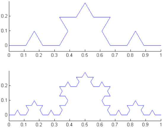
Figure 1.
K2 and K3.
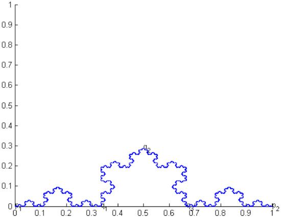
Figure 2.
Koch curve.
Let and for any sequence . Let be the union of the images of under these iterations. Let be a non-constant harmonic function on the (see [6], cf. [8], cf. [11], cf. [1], cf. [3]).
Lemma 1.
Given two numbers , there exists a unique non-constant harmonic function h on KC satisfying and .
Proof.
The proof is similar to the one of [3] (or [1]) and is omitted here. □
The graphs of harmonic functions on , and Koch curve (see Figure 3, Figure 4 and Figure 5) are given below. Compare and contrast them with Figure 4 of page 3233 in [6], where a graph of 1-nonconstant harmonic function on KC can be seen.
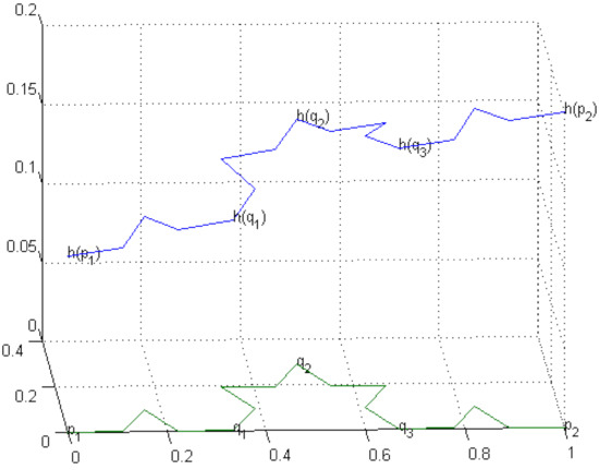
Figure 3.
A harmonic function on K2.
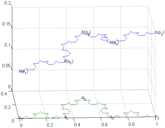
Figure 4.
A harmonic function on K3.
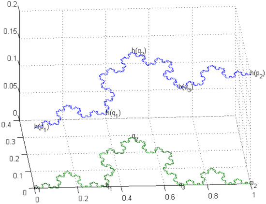
Figure 5.
A harmonic function on the Koch curve.
Without loss of generality, we may assume that (see [15], p. 314).
Theorem 4.
A harmonic function on is Hölder continuous.
Proof.
Since , for convenience, we assume that
Let and . Then, by the definition of non-constant harmonic function on , since for all , we obtain that
Let Then ,
On the other hand, since , we can see that and
By using the similar method, we can see that for all and ,
Also,
So, a harmonic function on is Hölder continuous. On the other hand, if , then h is not Hölder continuous function. In fact, we can easily see that since , inequality 1 is false. □
Now, we give certain IFSs on KC. Let be any given function (not necessarily a non-constant harmonic function on ), where (see [6]). Let be non-constant harmonic functions on the such that for ,
Then, by Lemma 1, for each , there exists a unique non-constant harmonic function on KC satisfying
Let be the IFS such that
where . Then we can see that for ,
Theorem 5.
If denotes the IFS defined above, then for any given numbers with , there exists a unique continuous function , such that ,
and
where and G is the graph of f.
Proof.
cf. [6]. □
The following motivation will be the key in the proof of Theorem 6.
- (1)
- Piecewise linear interpolation functions on an interval are special FIFs that are Lipschitz continuous (see [7], p. 212, p. 214), and so Lipschitz continuity with respect to the first variable x of functions and metrically equivalent metric are used in the proof of the uniqueness of invariant of IFS (see [7], p. 217, Theorem 1).
- (2)
- Harmonic functions on KC are special FIFs on KC (cf. [6], cf. [8]).
- (3)
- The graph of a constant harmonic function , is KC itself, and Hausdorff dimension of KC is , (see [2], p. 135, see [3]), and so box dimensions of graphs of non-constant harmonic functions on KC can be non-integers, and non-constant harmonic functions on KC can be Hölder continuous.
- (4)
- Since non-constant harmonic functions on KC are not Lipschitz continuous (see [8], p. 36), to obtain FIFs on KC as attractors of some IFSs is not possible from Barnsley’s fractal interpolation method.
- (5)
- The assertion that two metrics and are metrically equivalent is much stronger than the statement that they are topologically equivalent: to be metrically equivalent there must exist constants and such that for all ,and to be topologically equivalent must ensure that a sequence which is -convergent to is also -convergent to , and a sequence which is -convergent to is also -convergent to .
- (6)
- There can exist some metric d on , topologically equivalent (not necessarily metrically equivalent) to the Euclidean metric, such that IFS has a unique invariant set because the existence of metrically equivalent metric is a sufficient condition so that functions are Banach contractions with respect to some metric.
- (7)
- The results of [6,8] inspire us to ensure that graphs of FIFs generated on KC by non-constant harmonic functions of fractal analysis are attractors of some IFSs.
Our idea, based on the above motivation, is to use Hölder continuity of non-constant harmonic functions on KC and use some suitable metric which is topologically equivalent to the Euclidean metric but is not metrically equivalent to that.
Lemma 2.
(see [16]) If we consider a metric on by
where , and θ is some positive real number, then the metric is topologically equivalent to the Euclidean metric on .
Theorem 6.
Let denote the IFS defined above, associated with the points . Then there exists a unique nonempty compact set such that
Proof.
We define a metric on by
where , and . Since , by Theorem 4, for all ,
Hence we obtain for all and ,
Also, we obtain for all and ,
Since for all , and , we obtain that . Hence are Banach contractions in . So, for , there is a unique nonempty compact set such that
□
The graph of a fractal interpolation function on the Koch Curve (see Figure 6) is given below. Compare and contrast it with Figure 3 of page 3232 in [6], where the graph of a fractal interpolation function on KC is illustrated.
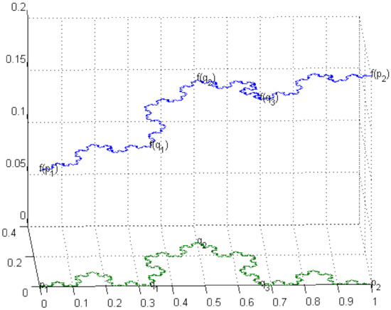
Figure 6.
A fractal interpolation function on the Koch curve (KC).
Please let us, apart from the above theorem, make some concluding remarks.
- (1)
- In the case of affine FIFs, functions are Lipschitz continuous with respect to the first variable x and are Banach contractions with respect to the second variable y becauseand
- (2)
- In the formulation and proof of Theorem 2, it is enough to assume that functions are continuous with respect to the first variable x and are Banach contractions with respect to the second variable y (see Theorem 2 in p. 218 of [7]), and in the formulation and proof of Theorem 5, it is enough to assume that functions are continuous with respect to the first variable x and second variable y and are Banach contractions with respect to the third variable z.
- (3)
- Theorems 2 and 5 do not ensure that the IFSs and have unique invariant sets. The uniqueness of invariant sets is determined explicitly in Theorems 3 and 6 (cf. the Theorem 1 in p. 217 of [7]).
- (4)
- In the formulation and proof of Theorem 6, it is needed to consider functions that are Hölder continuous with respect to the first variable x and second variable y and are Banach contractions with respect to the third variable z.
- (5)
- Theorem 3 is dedicated to show a sufficient condition for functions such that the IFS has a unique invariant set, and Theorem 6 is dedicated to show an essential sufficient condition for functions such that the IFS has a unique invariant set.
4. Discussion
One of the objectives would be to investigate how to optimise such a process in order to enhance mechanical properties of materials produced using the afore-mentioned method. The article [17] reports on the results of three studies investigating visual interest, visual preference, and mood responses elicited by varying complexities of fractal light patterns projected on walls and floors of an interior space. The article [18] presents a study on the design, and microstructural and mechanical characterization of additively manufactured reinforcing elements for composite materials exhibiting fractal geometry, with a focus on the flexural reinforcement of cement-matrix composites.
5. Conclusions
In this article, we used Hölder continuity of nonconstant harmonic functions on KC and a suitable metric, equivalent to the Euclidean metric, to prove Theorem 6. Moreover, we showed that it is possible to ensure that the graph of an FIF on KC by nonconstant harmonic functions of fractal analysis is the attractor of some IFS. An important fact is that the proof of the existence of fractal interpolation functions on the Koch curve is closely related to the same suitable iterated function system that generates the Koch curve, whereas a key result is that the proof of the uniqueness of FIFs depends not only on Hölder continuity of harmonic functions on the Koch curve but also on the topologically equivalent metric.
Author Contributions
Conceptualization, V.D.; methodology, S.-I.R.; software, S.-M.N.; supervision, S.-I.R. and V.D.; visualization, S.-M.N.; writing—original draft preparation, S.-I.R. and S.-M.N.; writing—review and editing, V.D. All authors have read and agreed to the published version of the manuscript.
Funding
This research received no external funding.
Data Availability Statement
Not applicable.
Acknowledgments
The authors would like to thank the reviewers for their efforts towards improving our manuscript.
Conflicts of Interest
The authors declare no conflict of interest.
References
- Kigami, J. Analysis on Fractals; Cambridge Tracts in Mathematics; Cambridge University Press: Cambridge, UK, 2001. [Google Scholar] [CrossRef]
- Massopust, P.R. Fractal Functions, Fractal Surfaces and Wavelets; Academic Press: San Diego, CA, USA, 1994. [Google Scholar]
- Strichartz, R.S. Differential Equations on Fractals: A Tutorial; Princeton University Press: Princeton, NJ, USA, 2006. [Google Scholar] [CrossRef]
- Drakopoulos, V.; Dalla, L. Space-filling curves generated by fractal interpolation functions. In Recent Advances in Numerical Methods and Applications II; Iliev, O., Kaschiev, M., Margenov, S., Sendov, B., Vassilevski, P., Eds.; World Scientific: Singapore, 1999; pp. 784–792. [Google Scholar] [CrossRef]
- Drakopoulos, V.; Tziovaras, A.; Böhm, A.; Dalla, L. Fractal interpolation techniques for the generation of space–filling curves. In Hellenic European Research on Computer Mathematics and Its Applications; Lipitakis, E.A., Ed.; LEA Press: Athens, Greece, 1999; pp. 843–850. [Google Scholar]
- Paramanathan, P.; Uthayakumar, R. Fractal interpolation on the Koch Curve. Comput. Math. Appl. 2010, 59, 3229–3233. [Google Scholar] [CrossRef]
- Barnsley, M.F. Fractals Everywhere, 3rd ed.; Dover Publications, Inc.: New York, NY, USA, 2012. [Google Scholar]
- de Amo, E.; Díaz Carrillo, M.; Fernández Sánchez, J. PCF self-similar sets and fractal interpolation. Math. Comput. Simul. 2013, 92, 28–39. [Google Scholar] [CrossRef]
- Ri, S.; Nam, S.; Kim, H. Fractal interpolation functions on affine fractal interpolation curves. Fractals 2021, 29, 2150046. [Google Scholar] [CrossRef]
- Agarwal, R.P.; O’Regan, D.; Sahu, D.R. Fixed Point Theory for Lipschitzian-Type Mappings with Applications; Springer: New York, NY, USA, 2009. [Google Scholar] [CrossRef]
- Çelik, D.; Şahin, K.; Özdemir, Y. Fractal interpolation on the Sierpinski Gasket. J. Math. Anal. Appl. 2008, 337, 343–347. [Google Scholar] [CrossRef][Green Version]
- Barnsley, M.F. Fractal functions and interpolation. Constr. Approx. 1986, 2, 303–329. [Google Scholar] [CrossRef]
- Tang, D. The Laplacian on p.c.f. self-similar sets via the method of averages. Chaos Solitons Fractals 2011, 44, 538–547. [Google Scholar] [CrossRef]
- Bedford, T. Hölder exponents and Box dimension for self-affine fractal functions. Constr. Approx. 1989, 5, 33–48. [Google Scholar] [CrossRef]
- Ri, S.G.; Ruan, H.J. Some properties of fractal interpolation functions on Sierpinski gasket. J. Math. Anal. Appl. 2011, 380, 313–322. [Google Scholar] [CrossRef]
- Ri, S. Fractal functions on the Sierpinski Gasket. Chaos Solitons Fractals 2020, 138, 110142. [Google Scholar] [CrossRef]
- Abboushi, B.; Elzeyadi, I.; Taylor, R.; Sereno, M. Fractals in architecture: The visual interest, preference, and mood response to projected fractal light patterns in interior spaces. J. Environ. Psychol. 2019, 61, 57–70. [Google Scholar] [CrossRef]
- Farina, I.; Goodall, R.; Hernández-Nava, E.; di Filippo, A.; Colangelo, F.; Fraternali, F. Design, microstructure and mechanical characterization of Ti6Al4V reinforcing elements for cement composites with fractal architecture. Mater. Des. 2019, 172, 107758. [Google Scholar] [CrossRef]
Publisher’s Note: MDPI stays neutral with regard to jurisdictional claims in published maps and institutional affiliations. |
© 2021 by the authors. Licensee MDPI, Basel, Switzerland. This article is an open access article distributed under the terms and conditions of the Creative Commons Attribution (CC BY) license (https://creativecommons.org/licenses/by/4.0/).