A Review on Fuzzy Cognitive Mapping: Recent Advances and Algorithms

Abstract

Fuzzy Cognitive Maps (FCMs) are a type of recurrent neural network with built-in meaning in their architecture, originally devoted to modeling and scenario simulation tasks. These knowledge-based neural systems support feedback loops that handle static and temporal data. Over the last decade, there has been a noticeable increase in the number of contributions dedicated to developing FCM-based models and algorithms for structured pattern classification and time series forecasting. These models are attractive since they have proven competitive compared to black boxes while providing highly desirable interpretability features. Equally important are the theoretical studies that have significantly advanced our understanding of the convergence behavior and approximation capabilities of FCM-based models. These studies can challenge individuals who are not experts in Mathematics or Computer Science. As a result, we can occasionally find flawed FCM studies that fail to benefit from the theoretical progress experienced by the field. To address all these challenges, this survey paper aims to cover relevant theoretical and algorithmic advances in the field, while providing clear interpretations and practical pointers for both practitioners and researchers. Additionally, we will survey existing tools and software implementations, highlighting their strengths and limitations towards developing FCM-based solutions.

1. Introduction

Fuzzy Cognitive Maps (FCMs) [1] originated as an advancement of cognitive maps, transforming a knowledge representation tool with limited capabilities into a versatile reasoning framework. In their canonical form, FCMs provide a tool for modeling complex systems, acknowledging that factors and their interrelationships are not strictly binary or linear in nature. The FCM field is currently actively developing and attracting interest from both researchers and practitioners, as evidenced by the recent publication of several textbooks [2,3].

Many of the initially reported applications of FCMs were devoted to simulation tasks in the realms of social science and psychology to represent and model cognitive processes and decision-making [4]. By the 1990s, FCMs began to be utilized in control systems [5] and complex systems [6] with ambiguous relationships. As the 2000s progressed, their versatility was recognized in the areas of sustainability and environmental modeling [7,8], social sciences [9,10], engineering [11,12,13,14,15], management [16,17,18,19,20], and healthcare [21,22,23,24,25]. FCMs have also been approached from a machine learning perspective, aiding in interpreting and modeling complex data structures and adaptive systems [26,27].

FCMs possess distinct features that make them more desirable than other deep learning models. First, FCMs allow for graded quantification of factors and relationships [28] while providing a graphical representation of the physical system under investigation [29,30]. Second, FCMs can serve as a bridge between technical experts and non-experts. Their graphical nature and ability to capture fuzzy relationships make them accessible for discussions between domain experts, decision-makers, and stakeholders from diverse backgrounds [31,32,33]. Third, FCMs are often considered interpretable due to their transparent structure, where each concept and causal relationship has a well-defined meaning, typically determined by experts. Nonetheless, their dynamic components, such as activation functions and reasoning rules, introduce complexity that can potentially reduce their interpretability. This dynamic nature challenges the assumption that FCMs are always intrinsically interpretable [34,35,36].

Building upon the strengths of FCMs, several extensions of these recurrent neural networks have been proposed in the literature [37]. For example, some works are inspired by extensions of the fuzzy sets theory, such as Hesitant Intuitionistic FCMs [38], fuzzy soft sets FCMs [39], or FCMs with Takagi-Sugeno-Kang fuzzy systems embedded [40]. Further extensions use mathematical frameworks, such as the k-valued FCMs [41] or the gray systems theory, for handling high-uncertainty scenarios [42,43,44]. Another line of studies hybridizes FCMs with other techniques for particular tasks, for example, deep graph convolution enhanced FCMs [45], a large reservoir of randomized high-order FCMs [46,47], community detection and FCMs for time series clustering [48], minimax concave penalty for FCMs in time series forecasting [49], or adding Bayesian methods to identify true causality [50]. Particularly promising is the extension of FCMs to federated learning settings, where the goal is to obtain privacy-preserving and securely distributed models [51,52]. Other studies attempt to correct or improve shortcomings of FCMs without resorting to hybrid models. For example, the revised modeling and simulation FCM methodology [53], which redefines the activation values in terms of quantity changes rather than absolute values.

Numerous papers have highlighted FCMs for their ability to handle ambiguity in designing very complex systems [54], but they are not without criticism. Several bad practices can undermine the effectiveness and reliability of FCMs. Constructing FCMs without involving domain experts can lead to inaccurate representations and the omission of key causal relationships. Arbitrarily assigning weights to the links without a systematic methodology or clear rationale compromises the model’s integrity. Oversimplifying complex systems by ignoring important variables or relationships can render the FCM ineffective, while overcomplicating it with unnecessary details can make it unwieldy and challenging to interpret. Failing to validate and update FCMs periodically, especially when new knowledge or data emerges, makes them outdated or misaligned with reality. Finally, overly relying on FCMs in scenarios where other tools might be more appropriate or ignoring the inherent subjectivity and qualitative nature of FCMs can lead to misguided decisions or conclusions [55]. These open challenges necessitate further research and refinement in the methodology and application of FCMs.

This literature review examines recent advancements in FCMs, with a focus on successful and robust methodologies. Analyzing the evolution of FCMs allows us to outline the field’s progression and the challenges it has faced. In the Appendix A, we summarize the search protocol used in this review, comprising databases, search queries, inclusion and exclusion criteria, and the screening process. In Figure 1, we depict the progression of the field based on the count of papers containing keywords related to FCMs in the title and abstracts, dating back to the foundational work of [1]. We can observe an apparent increase in the field’s activity, particularly in conjunction with classification and forecasting tasks, over the last decade.

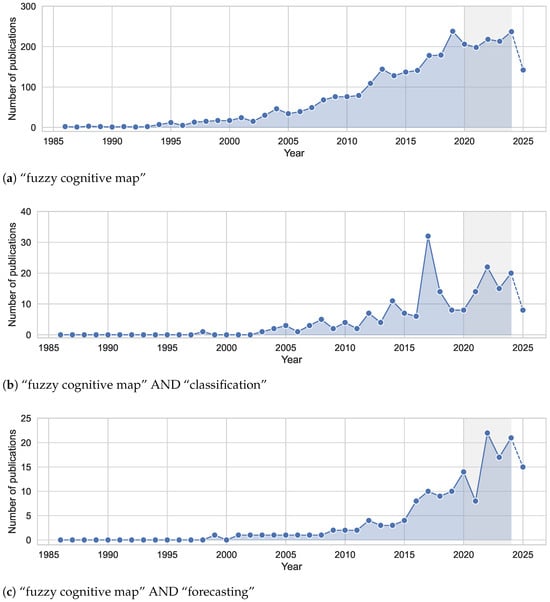
Figure 1. For each subfigure, we show the count of articles containing the keywords listed in its caption, either in the title or the abstract of the analyzed papers. Papers published after the foundational work of [1] are considered. The bibliometric data was extracted from https://app.dimensions.ai (accessed on 27 October 2025). For 2025, the statistics are included in dashed lines for the sake of completeness. The period highlighted in gray signals the last five years of publications.

Several review papers played key roles in highlighting recent advancements in the field. In [56], we find an overview of FCM-based time series forecasting models, Jiya et al. [57] presents a summary of learning approaches, Schuerkamp et al. [28] review popular extensions, and in [58] the authors cover aggregation strategies. In contrast, Felix et al. [59] offered an overview of numerous theoretical developments up to 2017. Given the dynamic and interdisciplinary nature of FCMs and the recent advances, this new literature review aims to update the community with consolidations made to the core foundations of FCMs, closing gaps and flaws that have been open for the last few decades. In particular, our review focuses on theoretical and algorithmic studies that have advanced FCMs as classifiers and time series forecasters, primarily over the past five years.

This paper aims to serve as a practitioner-oriented guide to building stronger FCM-based systems. Beyond surveying recent advances, we distill them into actionable design choices and guardrails: a standardized workflow for model construction (from concept elicitation and weight learning to activation and reasoning rules), diagnostic procedures to assess and enforce convergence, criteria for selecting learning families (metaheuristic, regression, and gradient) under data, noise, and compute constraints, and techniques for uncertainty handling, interpretability, and validation. We translate heterogeneous extensions (e.g., time-series forecasting, classification, gray/federated variants, and hybrid graph methods) into conclusions that clarify when each adds value and what trade-offs they impose. The result is a set of prescriptive best practices, a reporting checklist to enhance reproducibility and comparability, and references to available software tools that enable practitioners to transition from ad hoc FCM modeling to robust, auditable pipelines aligned with real-world requirements.

The rest of this paper is organized as follows. Section 2 presents a wrap-up of the different reasoning rules and activation functions utilized when building FCMs. Section 3 is dedicated to analyzing the various scenarios related to convergence (the process by which the system reaches a stable state after a series of iterations). Next, Section 4 analyzes learning methods, subdivided into metaheuristic-based, regression-based, and gradient-based approaches. Section 5 introduces the use of FCMs in time series forecasting problems. Section 6 addresses the adaptation of FCMs for pattern classification. Section 7 groups relevant software tools, libraries, and packages developed to design FCM-based models. Our review then presents our concluding remarks in Section 8.

2. Reasoning Rules and Activation Functions

This section will cover concept elicitation methods, the main reasoning rules, and theoretical results concerning the activation functions of these recurrent neural systems reported in the literature. Before discussing these topics, we will introduce the notation to be used in the paper.

Let N be the number of concepts in the FCM and T the maximum number of iterations, such that $t\in \{1,2,\dots ,T\}$ is the current iteration. The weight matrix defining the concept interaction is denoted as ${\mathbf{W}}_{N\times N}$. The activation vector containing the states of concepts in the current iteration is given by ${\mathbf{A}}_{1\times N}^{\left(t\right)}$. The activation vector in the t-th iteration is ${\mathbf{A}}^{\left(t\right)}=(a_1^{\left(t\right)},\dots ,a_i^{\left(t\right)},\dots ,a_N^{\left(t\right)})$ and gives the system state in the current iteration.

The initial activation vector is given by ${\mathbf{A}}^{\left(0\right)}=(a_1^{\left(0\right)},$$\dots ,a_i^{\left(0\right)},\dots ,a_N^{\left(0\right)})$. Therefore, the activation value of the i-th concept in the t-th iteration is $a_i^{\left(t\right)}$ such that $a_i^{\left(0\right)}$ is the initial activation value of that concept. The weight attached to the edge that departs from the i-th concept and arrives at the j-th concept is represented as $w_{ij}$. Furthermore, $f\left(x\right)$ represents the activation function that ensures the activation values of concepts are within the desired interval. Finally, ${\overline{\mathbf{A}}}^{\left(t\right)}=({\overline{a}}_1^{\left(t\right)},$$\dots ,{\overline{a}}_i^{\left(t\right)},$$\dots ,{\overline{a}}_N^{\left(t\right)})$ represents the raw activation vector, where ${\overline{a}}_i^{\left(t\right)}$ is the raw activation value of the i-th concept in the current iteration. In other words, the raw activation vector ${\overline{\mathbf{A}}}^{\left(t\right)}$ is the argument of the activation function attached to the reasoning rule.

2.1. Concept Elicitation

Concept elicitation plays a central role in the construction of FCMs, but the process differs significantly depending on whether the model is developed as a participatory scenario analysis tool or as a data-driven machine learning model. In their original formulation, FCMs were intended as tools for scenario analysis and participatory modeling [53]. Concept elicitation in this context is deeply intertwined with expert knowledge. Domain experts identify the key variables in the system, define the causal relations among them, and agree on the form of the activation function. What-if scenarios are encoded by assigning initial activation values to the relevant concepts, after which the recurrent reasoning procedure is applied to explore the consequences of these hypothetical situations. Knox et al. [32] published a comprehensive guide on eliciting concepts in a participatory setting. According to this paper, the quality of the model depends heavily on methodological choices such as whether concepts are elicited individually or in groups, whether the map is constructed directly by participants or facilitated by a moderator, whether concepts emerge through open-ended discussion, and whether modeling is performed with hand-drawn diagrams or dedicated software. Figure 2 depicts a workflow for building FCM models from historical data or in a participatory modeling setting.

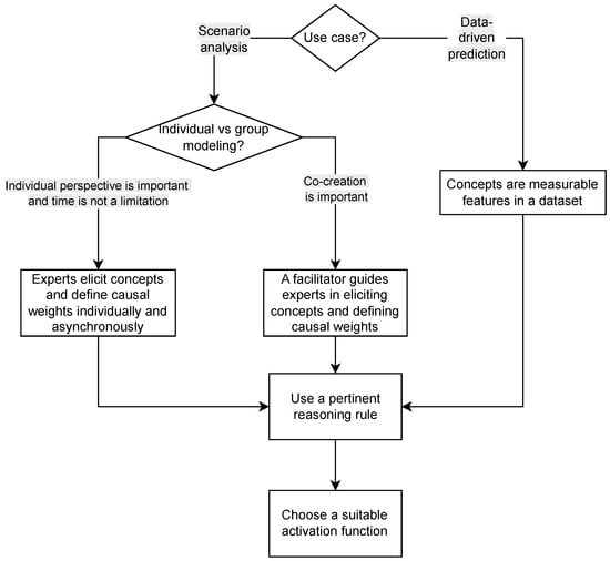
Figure 2. Workflow for building FCM models.

In contrast, when FCMs are used for tasks such as pattern classification, multi-output regression, or time series forecasting, the concept elicitation process shifts toward data-driven construction [53]. In these settings, concepts may correspond to measurable features in a dataset, and causal weights are learned automatically through dedicated training algorithms (see Section 4). The emphasis is no longer on participatory deliberation but on algorithmic extraction of structure from data. The resulting models often contain many more concepts and connections than expert-generated FCMs, and their interpretability depends on the ability to relate learned concepts and causal relations back to domain-understandable variables.

2.2. Reasoning Rules

The purpose of reasoning rules of FCM models is to iteratively update the concepts’ activation values given some initial conditions until a stopping criterion is met (see Figure 3). These rules employ three primary components to perform these calculations: the weight matrix, which indicates the connections between concepts, the activation values of concepts from the previous iteration, and the activation function. In this subsection, we will cover three state-of-the-art reasoning rules reported in the literature.

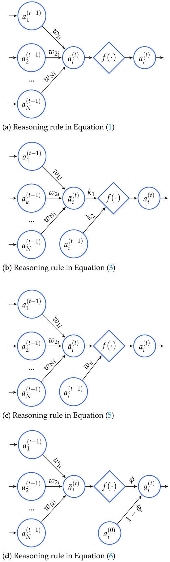
Figure 3. Reasoning rules for FCM models. In these diagrams, ${\overline{a}}_i^{\left(t\right)}$ denotes the raw activation value of the i-th concept in the current iteration, just before being transformed with the activation function.

Equation (1) shows the simplest reasoning rule widely employed by researchers and practitioners, which describes a first-order recurrence formula:

$$a_i^{\left(t\right)}=f\left(\sum _{j=1,i\ne j}^N{a}_j^{(t-1)}{w}_{ji}\right),$$

(1)

being equivalent to

$${\mathbf{A}}^{\left(t\right)}=f\left({\mathbf{A}}^{(t-1)}\mathbf{W}\right).$$

(2)

Equation (3) presents an extension of the reasoning rule in Equation (1) such that each concept uses its own past activation value when updating its state [60] in addition to the activation values of connected concepts,

$$a_i^{\left(t\right)}=f\left(k_1·\sum _{j=1,i\ne j}^N{a}_j^{(t-1)}{w}_{ji}+k_2·a_i^{(t-1)}\right),$$

(3)

being equivalent to

$${\mathbf{A}}^{\left(t\right)}=f\left(k_1·{\mathbf{A}}^{(t-1)}\mathbf{W}+k_2·{\mathbf{A}}^{(t-1)}\right),$$

(4)

such that $k_1$ regulates the impact of interconnected concepts on the new value for the i-th concept, while $k_2$ controls the extent to which the previous concept value contributes to the calculation of the new value. The two parameters $k_1$ and $k_2$ must satisfy the equation: $0<k_1,k_2\le 1$.

Hosseini et al. [61] used this extended reasoning rule (with $k_1=k_2$=1) in a hybrid FCM-based solution to estimate air over-pressure due to mine blasting. Similarly, Budak et al. [62] employed this reasoning rule to evaluate the impact of blockchain technology on the supply chain, while the author in [63] utilized this reasoning rule to carry through an FCM-based quality function deployment approach for dishwasher machine selection.

Stylios and Groumpos [60] presented another reasoning rule, especially devoted to FCM-based models, in which self-loops are implicitly allowed:

$$a_i^{\left(t\right)}=f\left(\sum _{j=1,i\ne j}^N{a}_j^{(t-1)}{w}_{ji}+w_{ii}·a_i^{(t-1)}\right),$$

(5)

being equivalent to Equation (2) where $\mathbf{W}$ has a non-zero diagonal. The reader can note that this reasoning rule is a particular case of Equation (3) where $k_1=1$ and $k_2=w_{ii}$ while dropping the constraint $0<k_1,k_2\le 1$.

This reasoning rule was employed by Qin et al. [64] to develop deep attention FCMs for interpretable multivariate time series prediction, by Yu et al. [65] to develop an FCM classifier based on capsule networks, and by Li et al. [66] to implement an intelligent stock trading decision support system based on rough cognitive reasoning, and by Shen et al. [67] to explore a new research avenue concerning evolutionary multitasking FCM learning.

The crux of these traditional reasoning rules above is that their behavior is fully controlled by the activation function $f(·)$ since all modifications happen before the function is applied to the raw activation values. As a result, we obtain models that might suffer from convergence issues while providing limited controllability. Aiming to address both issues, Nápoles et al. [68] proposed the quasi-nonlinear reasoning rule depicted below:

$$a_i^{\left(t\right)}=\underset{\mathrm{nonlinear}\mathrm{component}}{\underbrace{\varphi ·f\left(\sum _{j=1}^N{a}_j^{(t-1)}{w}_{ji}\right)}}+\underset{\mathrm{linear}\mathrm{component}}{\underbrace{\left(1-\varphi \right)·a_i^{\left(0\right)}}},$$

(6)

being equivalent to

$${\mathbf{A}}^{\left(t\right)}=\varphi ·f\left({\mathbf{A}}^{(t-1)}\mathbf{W}\right)+(1-\varphi )·{\mathbf{A}}^{\left(0\right)},$$

(7)

such that $0\le \varphi \le 1$ is the nonlinearity coefficient. When $\varphi =1$, the concept’s activation value depends on the activation values of connected concepts in the previous iteration. When $0<\varphi <1$, we add a linear component to the reasoning rule devoted to preserving the initial activation values of concepts. When $\varphi =0$, the model reduces to a linear regression where the initial activation values of concepts act as regressors.

A similar reasoning rule (that excluded the nonlinearity coefficient) was implemented into an FCM-based solution [69] to assess and manage the readiness for blockchain incorporation in the supply chain. In their paper, Nápoles et al. [68] used the quasi-nonlinear reasoning rule to quantify implicit bias in pattern classification datasets, while the authors in [70] resorted to this rule to develop a recurrence-aware FCM-based classifier. Similarly, Papadopoulos et al. [71] use it in the context of participatory modeling and scenario analysis for managing Mediterranean river basins.

The reader might reasonably wonder which reasoning rule is recommended when implementing FCM-based models. In that regard, the quasi-nonlinear reasoning rule in Equation (6) stands out as the preferred choice based on the following reasons. Firstly, it generalizes the remaining reasoning rules while controlling the relevance of the initial conditions when updating the activation values of the concepts. Secondly, it has appealing convergence properties (discussed in the next section), making it useful for various applications, including scenario analysis, time series forecasting, and pattern classification problems.

Last but not least, we note that a defining property of FCMs lies in recurrent signal processing, where the output passes back to the input until the termination criteria are satisfied. This behavior admits an interpretation as a refinement of the final system response. In that regard, the initial output of the model undergoes correction through a feedback loop. The moderating influence of this feedback depends on the weight values and can lead to distinct attractor regimes, with outcomes that range from irregular dynamics to convergence toward a fixed point. The literature discusses conditions for convergence in specific FCM-based models, for example [72,73,74].

2.3. Activation Functions

The activation function $f:\mathbb{R}\to I$ is an essential component in the reasoning rule of FCM-based models. This monotonically non-decreasing function keeps the activation value of each concept within the desired image set I, which can be discrete (a finite set) or continuous (a numeric-valued interval). It should be mentioned that I must be bounded; otherwise, the reasoning rule could explode due to the successive additions and multiplications when updating concepts’ activation values during reasoning. Table 1 portrays relevant activation functions found in the literature.

Table 1. Main discrete and continuous activation functions are used when implementing the reasoning rule of FCM-based models. For notation simplicity, x represents the concept’s raw activation value in a given iteration.

Equation	Description
$f\left(x\right)=\left\{\begin{array}{cc}1& ,x>0\\ 0& ,x\le 0\end{array}\right.$	The bivalent activation function [75] is a discrete activator that produces only two states (0 or 1). It allows modeling qualitative states, denoting whether a concept is active or not. Moreover, $f\left(0\right)=0$.
$f\left(x\right)=\left\{\begin{array}{cc}0& ,x\le v\\ 1& ,x>v\end{array}\right.$	The step activation function [76] is a discrete activator that generalizes the bivalent activation function. It allows for modeling qualitative states that denote whether a concept is activated or not, based on a threshold value v. In this function, $f\left(0\right)$ might not be zero.
$f\left(x\right)=\left\{\begin{array}{cc}-1& ,x<0\\ 0& ,x=0\\ 1& ,x>0\end{array}\right.$	The trivalent activation function [75] is a discrete activator that produces three states (−1, 0, 1). It allows for modeling qualitative states, denoting whether a concept is negatively activated, inactive, or positively activated. In this function, $f\left(0\right)=0$.
$f(x)=tanh(x)={\displaystyle \frac{e^{2x}-1}{e^{2x}+1}}$	The hyperbolic tangent function [75] is a continuous activator that produces infinite states within the ${[-1,1]}^N$ hypercube. This function can be used for modeling both qualitative and quantitative scenarios. Moreover, it is also true that $f\left(0\right)=0$. An extension using a threshold was introduced in [77].
$f(x)={\displaystyle \frac{1}{1+e^{-\lambda (x-h)}}}$	The sigmoid activation function [75] is a continuous activator that produces infinite states within the ${[0,1]}^N$ hypercube. $\lambda >0$ and $h\in \mathbb{R}$ are parameters controlling the function slope and offset, respectively. Higher $\lambda$ values increase the steepness, making it more similar to the bivalent activator. Positive h values shift the function to the right, while negative ones shift the function to the left. This function can be used for modeling both qualitative and quantitative scenarios. It should be noted that $f\left(0\right)$ might not be close to zero (see the discussion delivered by Mpelogianni et al. [78] about this issue and a proposed workaround).
$f\left(\mathbf{X}\right)=\left\{\begin{array}{cc}{\displaystyle \frac{\mathbf{X}}{{\left|\left|\mathbf{X}\right|\right|}_2}}\hfill & \mathrm{if}\mathbf{X}\ne \overrightarrow{0}\hfill \\ 0\hfill & \mathrm{otherwise}.\hfill \end{array}\right.$	The rescaled activation function [68] is a continuous activator that produces infinite states within the ${[-1,1]}^N$ hypercube. It has a zero intercept and can be used to model qualitative and quantitative scenarios. Instead of operating on a single concept, this activator receives a vector with the activation values of the concepts to be transformed. These raw activation values are divided by the Euclidean norm of the vector to obtain the concepts’ activation values.
$f\left(x\right)=sgn\left(x\right)\ast \left(\right|x|/{\sum }_{j=1}^N|w_{ji}{\left|\right)}^{\beta }$	The exponential normalized activation function [53] was introduced as part of a revised methodology for simulation with FCMs. This activation function accounts for the activation values of negative and positive concepts, denoting changes. It addresses the saturation issues where neural concepts are assigned values close to the extremes of the activation space. This function also provides modelers with the flexibility to control the nonlinearity of simulations through the parameter $\beta$, allowing for a transition from linear to exponential behavior.

Overall, continuous activators, such as the sigmoid, the hyperbolic tangent, and the rescaled activation functions, are often preferred since they provide greater expressiveness. Actually, the study in [76] advocated for using the sigmoid activation function when modeling scenario analysis problems over the hyperbolic tangent and threshold functions. However, the rescaled function requires further study and comparison with other functions in terms of their approximation capabilities and expressiveness.

3. Convergence Analysis and Theoretical Studies

As for the stopping criteria, the reasoning rules stop when either (i) the model converges to a fixed point or (ii) a maximal number of iterations T is reached. Overall, we have three possible states:

• Fixed point $(\exists t_{\alpha }\in \{1,\dots ,(T-1)\}:a_i^{(t+1)}=a_i^{\left(t\right)},\forall i,\forall t\ge t_{\alpha })$: the FCM produces the same activation vector after $t_{\alpha }$, implying that a fixed point was found. As a result, $a_i^{\left(t_{\alpha }\right)}=a_i^{(t_{\alpha }+1)}=a_i^{(t_{\alpha }+2)}=\cdots =a_i^{\left(T\right)}$.
• Limit cycle $(\exists t_{\alpha },P,j\in \{1,\dots ,(T-1)\}:a_i^{(t+P)}=a_i^{\left(t\right)},$$\forall i,\forall t\ge t_{\alpha })$: the FCM produces the same activation vector with period P, thus $a_i^{\left(t_{\alpha }\right)}=a_i^{(t_{\alpha }+P)}=a_i^{(t_{\alpha }+2P)}=\cdots =a_i^{(t_{\alpha }+jP)}$, where $t_{\alpha }+jP\le T$.
• Chaos: the FCM produces different activation vectors for successive iterations, which makes decision-making difficult.

It is worth noting that fixed-point attractors can be categorized into two main types: unique fixed points and multiple fixed points. If the fixed point is unique, then the FCM model will produce the same solution regardless of the initial conditions. The FCM model can create multiple solutions if multiple fixed points exist. Two seminal theoretical results concerning the convergence of FCM models to unique fixed points paved the road for recent developments.

The first of these theoretical results was introduced by Boutalis et al. [79] and concerns two theorems (see Theorems 1 and 2) on the stability of sigmoid FCMs. While the first theorem focuses on FCM models without inputs, the second assumes that some concepts influence others but are not influenced by any other concepts. In both cases, the theorems provide conditions related to the existence and uniqueness of the fixed-point attractors.

Theorem 1.

There exists one and only one solution for any activation value $a_i$ of any sigmoid FCM if the following expression holds:

$${\left(\sum _{i=1}^N∥w_i∥\right)}^{1/2}<4.$$

Theorem 2.

For a sigmoid FCM with M input concepts, there exists one and only one solution for any activation value $a_i$ if the following expression holds:

$${\left(\sum _{i=1}^{N-M}∥w_{M+i}∥\right)}^{1/2}<4.$$

We recognize these theorems as the first successful attempt to determine mathematical conditions related to the existence and uniqueness of fixed points of FCMs using the sigmoid activation function $f\left(x\right)=1/(1+e^{-\lambda x})$ with $\lambda =1$. Kotas et al. [80] attempted to generalize these theorems for arbitrary sigmoid functions, allowing the inclination parameter $\lambda$ to vary. Although their approach was initially accepted by the community and cited several times (for example, in the previous review paper by [59]), it was ultimately refuted by numerical counterexamples in [81]. Harmati et al. [82] correctly generalized these theorems for arbitrary $\lambda$ values, as Theorem 3 shows. Moreover, they extended the analysis to FCM models that utilize the hyperbolic tangent function and examined the case of FCMs equipped with non-negative weight matrices, applying Tarski’s fixed-point theorem.

Theorem 3.

Let $\mathbf{W}$ be the extended weight matrix of an FCM, and let $\lambda >0$ be the parameter of the log-sigmoid activation function. If the inequality

$${\left|\right|\mathbf{W}\left|\right|}_F<{\displaystyle \frac{4}{\lambda }}$$

holds, then the FCM has one and only one fixed point. In the formula, ${\left|\right|.\left|\right|}_F$ refers to the Frobenius norm of the matrix, i.e., ${\left|\right|\mathbf{W}\left|\right|}_F={\left({\sum }_i{\sum }_j{w}_{ij}^2\right)}^{1/2}$.

The second seminal theoretical result concerning the existence and uniqueness of the fixed point was presented in [83], where the authors proved that the slope of the activation function determines the number of attractors in a sigmoid FCM (see Theorem 4). From an analytical viewpoint, this theorem could be considered a variation of Theorems 1 and 2. However, Theorem 4 focuses on the properties that the sigmoid activation function must satisfy for the map to be linearly stable.

Theorem 4.

The number of fixed points of a sigmoid FCM model depends on the slope λ of the activation function.

(a) 

If $\lambda \ge 0$ is sufficiently small, then the map will have a unique solution, and this solution will be linearly stable.

(b) 

If $\lambda \ge 0$ is sufficiently large, then the map will have multiple solutions, and many of these solutions can be linearly stable.

Knight et al. [83] mathematically defined bounds to elucidate what is considered “small enough” in Theorem 4, removing all sources of ambiguity.

Theorem 5.

For $\mathbf{W}\in {\mathbb{R}}^{N\times N}$ and h given, the sigmoid FCM has a unique fixed point for all λ such that $0\le \lambda \le \overline{\lambda }\left(N\right)$, this fixed point is stable.

$$\begin{array}{c}\hfill {\left(1-{\displaystyle \frac{\overline{\lambda }\left(N\right)}{4}}\right)}^N-\sum _{i=1}^N{b}_i{C}_i^N{\left({\displaystyle \frac{\overline{\lambda }\left(N\right)}{4}}\right)}^i=0\end{array}$$

where $C_i^N$ are the binomial coefficients, and $b_i$ is given by the recursion relation $b_i=i{b}_{i-1}+{(-1)}^i,b_0=1$.

Recently, Harmati et al. [81] improved the above analytical results. Concerning the results presented by Boutalis et al. [79] extended in [82], they explained that we could find a matrix norm ${\parallel ·\parallel }_{*}$, such that ${\parallel W\parallel }_{*}\le {\parallel W\parallel }_F$. The ramification of this remark is that the global convergence to a unique fixed point is proved for a larger set of $\lambda$ values. Concerning the results in Knight et al. [83], they provided more realistic bounds to define what is considered “small enough", as formalized in the theorems below.

Theorem 6.

Consider a sigmoid FCM with weight matrix $\mathbf{W}\in {\mathbb{R}}^{N\times N}$ and sigmoid parameter λ. If $0\le \lambda <{\displaystyle \frac{4}{N}}$, then the FCM has a unique and globally asymptotically stable fixed point.

Theorem 7.

Let $\overline{\lambda }\left(N\right)$ be defined as in Theorem 5. Then, the inequality $\begin{array}{c}\hfill \overline{\lambda }\left(N\right)\le {\displaystyle \frac{4}{N}}\end{array}$ holds for every $N\ge 1$.

Such an upper bound is easier to compute while ensuring the uniqueness of fixed points for a larger set of $\lambda$ values. The authors also stated that no better upper bound can be estimated by using a different norm. However, their method is flexible enough to increase the upper bound provided, allowing for more information about the weights to be available. Harmati et al. [81] also discussed the superiority of their approach when compared with the Lyapunov stability analysis conducted by Lee et al. [84].

While these analytical results have enhanced our understanding of the convergence properties of FCM models, the practical usability of the unique fixed point is limited. In other words, FCM models converging to a unique fixed point are unsuitable for performing what-if scenario analysis or solving prediction problems (such as regression, time series forecasting, or pattern classification). The authors in [85] first discussed this issue and experimentally illustrated how an FCM-based classifier will only recognize a single decision class when the model converges to a unique fixed point. Harmati et al. [81] also provided a clear statement about this issue, which reads as follows: “The results presented in this paper can be used in at least two different ways: in some applications, a unique fixed point is a required property of the model. It means that different initial stimuli should lead to the same equilibrium state. On the other hand, there are applications (for example, pattern recognition) where the FCM should have more than one equilibrium point. In other words, global stability is a required property in the first case, while in the second case, we should avoid globally stable models. The simple analytical results help FCM users decide about some model parameters before evaluating the full model, decreasing the number of trial-and-error simulations.”

In [86], the authors proposed a mathematical formalism to study the effectiveness of learning algorithms devoted to improving the convergence properties of FCM models. In that regard, the authors introduced the concepts of E-stability and E-instability along with sufficiency conditions for these properties.

Definition 1.

We say that an FCM, where the i-th concept uses the sigmoid activation function $f(x,{\lambda }_i,h_i)=1/(1+e^{-{\lambda }_i(x-h_i)})$, is E-accurate in the t-th iteration if each concept $C_i$ is ${\xi }_i$-accurate, where $E=\left\{{\xi }_1,\dots ,{\xi }_i,\dots ,{\xi }_N\right\}$ and ${\xi }_i\in [0,1]$. Moreover, a sigmoid concept $C_i$ is deemed accurate ξ-accurate in the t-th iteration if $|a_i^{\left(t\right)}-a_i^{\left(T\right)}| \le {\xi }_i$, where ${\xi }_i\in [0,1]$.

Definition 2.

We say that an FCM, where the i-th concept uses the sigmoid activation function $f(x,{\lambda }_i,h_i)=1/(1+e^{-{\lambda }_i(x-h_i)})$, is E-stable if $\exists t_q\in \mathbb{N}:\forall i\forall t\ge t_q$ such that $|a_i^{\left(t\right)}-a_i^{\left(T\right)}| \le {\xi }_i$, where $E=\left\{{\xi }_1,\dots ,{\xi }_i,\dots ,{\xi }_N\right\}$ and ${\xi }_i\in [0,1]$. Otherwise, the FCM is said to be E-unstable.

Remark 1.

The previous definitions (and consequently the theorems below) hold for a collection of initial activation vectors used to start the recurrent reasoning process. However, we decided to omit the subscript indexing the initial activation vectors to lighten the notation.

Theorem 8.

(Sufficiency Condition). A sigmoid FCM will be E-stable if the following conditions are simultaneously satisfied:

(a) 

$\left(|a_i^{\left(t\right)}-a_i^{\left(T\right)}|\le {\xi }_i\right)\Rightarrow \left(|MI{N}_i-a_i^{\left(T\right)}|\le {\xi }_i\right)\wedge \left(|MA{X}_i-a_i^{\left(T\right)}|\le {\xi }_i\right),\forall i$

(b) 

$\exists t_q\in \mathbb{N}$ such that the FCM is E-accurate in the $t_q$-th iteration

where

$$MI{N}_i=f({\mathit{W}}_i{\mathit{A}}^{\left(T\right)}+min\left({\mathit{W}}_i{\mathit{D}}^{\left(t\right)}\right),{\lambda }_i,h_i)$$

$$MA{X}_i=f({\mathit{W}}_i{\mathit{A}}^{\left(T\right)}+max\left({\mathit{W}}_i{\mathit{D}}^{\left(t\right)}\right),{\lambda }_i,h_i)$$

and ${\mathit{W}}_i=(w_{i1},\dots ,w_{iN})$ represents the i-th row of the weight matrix, ${\mathit{A}}^{\left(T\right)}=(a_1^{\left(T\right)},\dots ,a_i^{\left(T\right)},\dots ,a_N^{\left(T\right)})$ is the vector of expected responses for a given initial activation vector, ${\mathit{D}}^{\left(t\right)}=(d_1^{\left(t\right)},\dots ,d_i^{\left(t\right)},\dots ,d_N^{\left(t\right)})$ with $|d_i^{\left(t\right)}|\le {\xi }_i$, and $min\left({\mathit{W}}_i{\mathit{D}}^{\left(t\right)}\right)$ and $max\left({\mathit{W}}_i{\mathit{D}}^{\left(t\right)}\right)$ are defined as follows:

$$min\left({\mathit{W}}_i{\mathit{D}}^{\left(t\right)}\right)=\sum _{j=1}^N-\mathit{sgn}\left(w_{ij}\right)w_{ij}{\xi }_i$$

$$max\left({\mathit{W}}_i{\mathit{D}}^{\left(t\right)}\right)=\sum _{j=1}^N\mathit{sgn}\left(w_{ij}\right)w_{ij}{\xi }_i.$$

Theorem 9.

(Sufficiency Condition). A sigmoid FCM will be E-unstable if the following condition is satisfied:

$$\left(|a_i^{\left(t\right)}-a_i^{\left(T\right)}|\le {\xi }_i\right)\Rightarrow \exists j:\left(a_j^{\left(T\right)}<MI{N}_j-{\xi }_j\right)\vee \left(a_j^{\left(T\right)}>MA{X}_j+{\xi }_j\right),\forall i$$

where

$$MI{N}_j=f({\mathit{W}}_j{\mathit{A}}^{\left(T\right)}+min\left({\mathit{W}}_j{\mathit{D}}^{\left(t\right)}\right),{\lambda }_j,h_j)$$

$$MA{X}_j=f({\mathit{W}}_j{\mathit{A}}^{\left(T\right)}+max\left({\mathit{W}}_j{\mathit{D}}^{\left(t\right)}\right),{\lambda }_j,h_j)$$

Remark 2.

Similarly, to Theorem 8, $MI{N}_j$ and $MA{X}_j$ define the interval in which $a_j^{(t+1)}$ varies. If $\exists j:\left(a_j^{\left(T\right)}<MI{N}_j-{\xi }_j\right)\vee \left(a_j^{\left(T\right)}>MA{X}_j+{\xi }_j\right)$, then the FCM with $f(x,{\lambda }_i,h_i)=1/(1+e^{-{\lambda }_i(x-h_i)})$ will not be E-accurate in the $(t+1)$-th iteration, and therefore, it cannot be E-stable.

The authors in [86] also proposed sufficient conditions for FCM-based models where ${\lambda }_i\in [{\lambda }_{MIN},{\lambda }_{MAX}]$ and $h_i\in [h_{MIN},h_{MAX}],\forall i$. The ramification of these analytical results is that algorithms devoted to improving the convergence properties of FCM models a posteriori [85] have limited effectiveness if no modifications are made to the weight matrix.

The study in [87] proposed another mathematical framework to study the dynamic behavior of FCMs with monotonically increasing functions bounded. They proved that the state space of an FCM shrinks infinitely and converges to a so-called limit state space, which could be a fixed-point attractor. In that regard, we can determine whether the fixed-point attractor will be unique or not. The relevance of this result is that we can determine the feasible activation space of each concept in advance, regardless of the initial activation vectors. Moreover, the fact that the feasible activation space of a neural concept is smaller than the theoretically possible activation space $[0,1]$ indicates that values outside the feasible activation space will never be reached. Later, Concepción et al. [88] extended these results to quasi-nonlinear FCM models.

These bounds enable practitioners to design realistic decision support systems or predictive models, as most real-world applications must avoid unique fixed-point attractors. In this regard, Nápoles et al. [68] introduced a theorem that gives conditions (related to the nonlinearity coefficient) for which the quasi-nonlinear reasoning rule in Equation (7) will never converge to a unique fixed-point attractor. Following a different research direction, the authors in [89] used these analytical lower and upper bounds to design a supervised learning algorithm that does not require any training data.

Theorem 10

(Injective convergence). In an FCM model using Equation (7), when $0\le \varphi <1$, there are not two different initial activation vectors leading to the same fixed-point attractor.

If the coefficient $\varphi$ is set to 1.0, the convergence behavior of the FCM will depend on the activation function. For example, suppose we adopt the rescaled activation function. In that case, the model will undoubtedly converge to a unique fixed-point attractor provided that (i) the transposed weight matrix has an eigenvalue that is strictly greater in magnitude than other eigenvalues, and (ii) the initial activation vector has a nonzero component in the direction of an eigenvector associated with the dominant eigenvalue.

The literature reports other studies concerning the convergence of Fuzzy-Rough Cognitive Networks [90,91], the algebraic dynamics of k-valued FCMs [92], or the behavior of gray or interval-valued FCMs [73,74,93]. However, this section does not describe these studies in detail, since they focus on FCM extensions with specific topologies and knowledge structures. Concerning algorithmic approaches, [72] employed supervised and unsupervised learning to improve the model convergence for operational risk assessment in power distribution networks.

Convergence Analysis Illustration

An inspection of the literature reveals that the sigmoid activation function is the preferred choice among practitioners and researchers alike when designing FCM-based models. After all, previous benchmarking studies [75,76] claimed its superiority over other activation functions such as binary, trivalent, or hyperbolic tangent functions. However, only a few studies [53,85,94] have discussed the risks posed by the sigmoid function when it comes to the system’s convergence to unique fixed-point attractors. We must emphasize that these invariant equilibrium points render the FCM model ineffective for performing any simulation or predictive task and must be avoided at all costs.

This subsection presents two hypotheses that are empirically investigated. First, we conjecture that any FCM model using the reasoning rules in Equations (1) and (3) and the sigmoid function with $\lambda =1.0$ will converge to a unique fixed point. Second, we hypothesize that increasing the $\lambda$ value will help escape from the unique fixed point for larger, more densely connected FCMs at the expense of biasing the neurons’ activation values toward the extremes of the activation interval.

Aiming to investigate our hypotheses, we first generated 10,000 networks such that the number of concepts is $N\backsim U(2,20)$ and the number of edges is $M\backsim U((N^2-N)/10,(N^2-N))$, which translates into a ratio of edges ranging from 0.1 (simulating sparse models as the one for scenario analysis) to 1.0 (simulating dense models as the ones used for prediction tasks). The main diagonal of these weight matrices was filled with zeros to avoid explicit self-loops and the remaining non-zero elements were given by $w_{ij}\backsim U(-1,1)$ under the assumption that ${\sum }_j\left|w_{ij}\right|\ne 0,\forall i$. In addition, for each FCM model, we generated 100 initial activation vectors, such that $a_i^{\left(0\right)}\backsim U(0,1)$. In the simulation step, we applied both reasoning rules to each model using the randomly generated initial conditions while varying the $\lambda$ parameter from 1.0 to 5.0, totaling 10 million simulations. In all cases, the maximal number of iterations was set to $T=50$. Concerning convergence, we say that the fixed point is unique for a given model if $max\left\{\right||{\mathbf{A}}_i^{\left(T\right)}-{\mathbf{A}}_j^{\left(T\right)}|{|}_2<1.0\times {10}^{-4}\},\forall i,j$ such that ${\mathbf{A}}_i^{\left(T\right)}$ and ${\mathbf{A}}_j^{\left(T\right)}$ denote the final activation vectors obtained for the i-th and j-th initial activation vectors, respectively.

Figure 4 depicts the unique fixed-point attractors produced for both reasoning rules and different $\lambda$ values when increasing the number of concepts and the ratio of edges. In this figure, the white spaces correspond to multiple fixed points, limit cycles, and chaotic states.

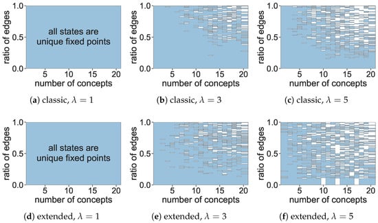
Figure 4. Unique fixed points for different settings.

The simulations indicate that all models converged to a unique fixed point when $\lambda =1.0$ for both reasoning rules. This result is concerning since such a parametric setting is the default setting in FCM research, thus leading to models with no simulation or predictive capability. Increasing the $\lambda$ value helps alleviate this issue to some extent. However, regular-sized FCMs (i.e., with less than 10 concepts) having connectivity up to 50% will be at risk of converging to a unique fixed point when using the classic reasoning rule. In contrast, the extended reasoning rule seems to be less likely to produce invariant fixed points for larger $\lambda$ values.

Figure 5 shows the distribution of concepts’ activation values in the last iteration when using different reasoning rules and $\lambda$ values. These results reveal why using the extended reasoning rule and large $\lambda$ values is not generally advised, even when they help the FCMs escape from unique fixed points. Firstly, this reasoning rule is biased toward producing larger activation values compared to the classic rule, since smaller values are less likely to be produced. Secondly, larger inclination values cause the function to behave like a quasi-binary activator, which translates into a significant loss in precision. Moreover, the fact that these final activation values are not uniformly distributed for any of these settings suggests that the FCM models might struggle to approximate any value in the activation interval. In that regard, using unbounded weights could lead to better results.

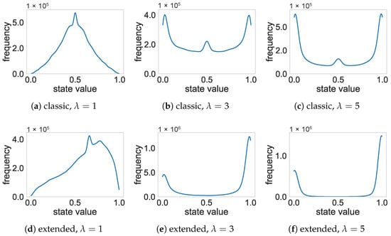
Figure 5. Distribution of activation values for different settings.

These experiments made clear that the classic and extended reasoning rules coupled with the sigmoid activation function (using $\lambda =1.0$) should not be used and that larger inclination values might still lead to unique fixed points. Hence, it would be useful to derive a mathematical tool to determine whether an FCM model will converge to a unique fixed point based on the weight matrix only, regardless of the initial activation vector. To do that, we will rely on the theory presented in Concepción et al. [87] to describe the feasible activation space of each neural concept.

Let ${\mathcal{I}}_i^{\left(0\right)}=[{inf}_i^{\left(0\right)},{sup}_i^{\left(0\right)}]$ be the feasible activation space for the i-th neural concept when starting the recurrent reasoning process, where ${inf}_i^{\left(0\right)}=0$ and ${sup}_i^{\left(0\right)}=1$ represent the lower and upper bounds, respectively. To derive the feasible activation space ${\mathcal{I}}_i^{(t+1)}=[{inf}_i^{(t+1)},{sup}_i^{(t+1)}]$ associated with the i-th neural concept in the $(t+1)$-th iteration, we will assume that $f(·)$ is a continuous, bounded, non-negative, and monotone-increasing activation. The sigmoid activation function addressed in this note fulfills these properties. Afterwards, we need to calculate the minimum and maximum bounds for the dot product ${\mathbf{w}}_i{\mathbf{A}}^{\left(t\right)}$, as formalized below:

$$min\left({\mathbf{w}}_i{\mathbf{A}}^{\left(t\right)}\right)={\displaystyle \frac{1}{2}}\sum _{j=1}^N{w}_{ji}\left({\sup }_j^{\left(t\right)}\left(1-\mathrm{sgn}\left(w_{ji}\right)\right)+{\inf }_j^{\left(t\right)}\left(1+\mathrm{sgn}\left(w_{ji}\right)\right)\right)$$

(8)

$$max\left({\mathbf{w}}_i{\mathbf{A}}^{\left(t\right)}\right)={\displaystyle \frac{1}{2}}\sum _{j=1}^N{w}_{ji}\left({\sup }_j^{\left(t\right)}\left(1+\mathrm{sgn}\left(w_{ji}\right)\right)+{\inf }_j^{\left(t\right)}\left(1-\mathrm{sgn}\left(w_{ji}\right)\right)\right)$$

(9)

such that ${inf}_j^{\left(t\right)}$ and ${sup}_j^{\left(t\right)}$ represent the bounds (infimum and supremum, respectively) of the closed interval ${\mathcal{I}}_j^{\left(t\right)}$ attached to the j-th neural concept. Therefore, it holds that ${{inf}_j}^{\left(t\right)}\le a_j^{\left(t\right)}\le {{sup}_j}^{\left(t\right)},\forall j.$ Inductively, we can compute ${inf}_i^{(t+1)}$ and ${sup}_i^{(t+1)}$ as indicated below:

$${{inf}_i}^{(t+1)}=f\left(min\left({\mathbf{w}}_i{\mathbf{A}}^{\left(t\right)}\right)\right)$$

(10)

$${{sup}_i}^{(t+1)}=f\left(max\left({\mathbf{w}}_i{\mathbf{A}}^{\left(t\right)}\right)\right).$$

(11)

At the model level, the Cartesian product of all these feasible activation spaces creates a feasible state space ${\mathcal{S}}^{(t+1)}={\mathcal{I}}_1^{(t+1)}\times {\mathcal{I}}_2^{(t+1)}\times \dots \times {\mathcal{I}}_N^{(t+1)}$ at the $(t+1)$-th iteration. Therefore, we can confidently conclude that the FCM model will converge to a unique fixed point if ${{sup}_i}^{(t+1)}-{{inf}_i}^{(t+1)}<\xi ,\forall i$ regardless of the concepts’ initial activation values.

Aiming to illustrate the usability of this formalism, let us compute the lower and upper bounds for each neural concept in the FCM model introduced in [95]. Figure 6 shows this model, which involves 17 relationships, from which 6 are positive (solid lines), and 11 are negative (dashed lines). In this case, the network density is 21%, which indicates that the weight matrix has 17 out of 81 non-zero causal relationships.

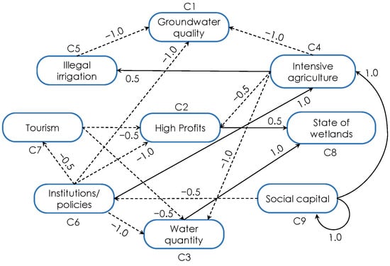
Figure 6. FCM model for European freshwater resource development.

Figure 7 depicts the concepts’ lower and upper bounds in each iteration. These bounds indicate that the FCM will always converge to a unique fixed point regardless of the initial activation vectors.

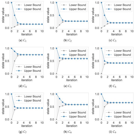
Figure 7. Lower and upper bounds for the neural concepts in the European freshwater FCM model. After five iterations, the model converged to a unique fixed point since ${{sup}_i}^{(t+1)}-{{inf}_i}^{(t+1)}<1.0\times {10}^{-4}$ for all i and all $t\ge 5$.

This subsection highlights significant issues with using the sigmoid activation function in FCM-based models, particularly concerning the convergence to unique fixed-point attractors. Our findings strongly suggest that neither the classic nor the extended reasoning rules must be used together with the sigmoid activation function with $\lambda =1.0$. In case this combination would be nonetheless used for larger $\lambda$ values, we described a mathematical formalism to determine whether a particular FCM model will converge to a unique fixed point, irrespective of the initial activation vector. Alternatively, we strongly recommend utilizing the quasi-nonlinear reasoning rule, which is compatible with any activation function, including the sigmoid, and does not produce unique fixed-point attractors.

Another alternative is to resort to the neural cognitive methodology presented in [53], where activation values denote quantity changes rather than absolute values. Figure 8 shows a flow diagram depicting how to interpret the simulation results in the presence of different convergence behaviors.

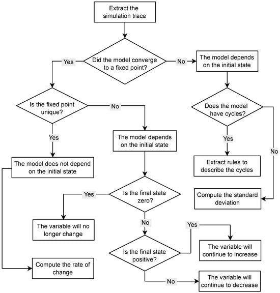
Figure 8. Workflow for interpreting FCMs simulation results in terms of increase and decrease of variables, in relation to different convergence scenarios [53].

The reader can note that such a methodology covers all dynamic cases, including meaningful interpretations of unique fixed-point attractors.

4. Learning Algorithms and Taxonomy

The literature on learning algorithms for FCM-based models is rich and sometimes disorganized. Our study of the current approaches has led us to propose a taxonomy of the existing error-driven FCM learning strategies (see Figure 9). According to the target learnable parameters, existing algorithms can be gathered into two broad categories: synaptic and nonsynaptic. Synaptic learning is oriented toward fitting the weight values that characterize the relationships between neural entities. Nonsynaptic learning utilizes previously defined weights and adjusts other model parameters, including the activation functions and network topology. Later subsections address prominent learning algorithms used for both synaptic and nonsynaptic learning.

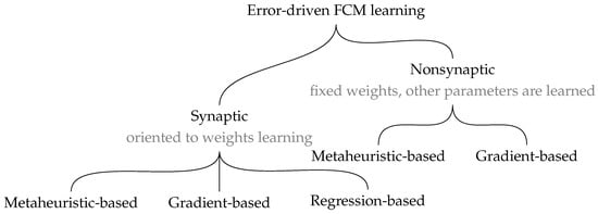
Figure 9. Error-driven learning of FCM models. The plot illustrates the division of current FCM learning techniques.

More explicitly, we will cover metaheuristic-based algorithms (both standard methodologies and recent methods) and some relevant objective functions that drive the search process. Moreover, we will cover regression-based and gradient-based algorithms, which are deemed a new generation of learning algorithms for FCM-based models.

4.1. Metaheuristic-Based Learning Algorithms

A significant body of research on FCM construction employs metaheuristic approaches to compute the weight matrix and, when applicable, optimize additional parameters [96]. Firstly, let us briefly emphasize that metaheuristic optimization aims to identify a solution to a problem that meets a “sufficiently good” criterion. This criterion is typically measured using an objective function. Importantly, there is no guarantee of discovering an optimal solution. Nevertheless, in many engineering applications, such an assumption proves satisfactory in yielding effective solutions. The research community has rapidly embraced the simplicity of this practical goal, resulting in the development of numerous algorithms that align with this rationale.

While heuristic methods have been in use for over 20 years, as indicated by the early approaches [97], studies continue to employ these methodologies without significant modification. The three key categories of well-studied heuristic methods in FCM development include (i) Genetic Algorithms (GAs), (ii) other evolutionary algorithms, and (iii) swarm-based methods such as Particle Swarm Optimization (PSO) and others.

In the following subsection, we will discuss relevant approaches to metaheuristic-based learning of FCM models used in studies from 2016 to 2023. Whenever opportune, we will include papers that extend beyond this time period to ensure completeness in our review.

4.1.1. Standard Methodologies Used up to This Day

One renowned “old” methodology in contemporary literature is rooted in the GA paradigm, as discussed by Hoyos et al. [98]. Typically, the model’s structure aligns with a basic FCM model, akin to the method by Altundoğan and Karaköse [99]. Nevertheless, other FCM extensions have also been referenced. For example, Hajek and Prochazka [100] employed interval-valued FCMs combined with genetic learning to predict corporate financial distress. Other approaches move beyond prediction tasks, such as the study delivered by Rotshtein et al. [101], who focused on conducting “what if" scenario analysis in an FCM-based model of the Ukraine-Russia war. Earlier studies include applications such as computer-aided medical diagnosis [102].

The second category of heuristic searches, introduced at the beginning of studies on FCM data-driven development and still in use in an unchanged form, comprises other evolutionary approaches. For example, a study by Hosseini et al. [103] utilized a Differential Evolution (DE) algorithm. Additionally, new variants of this approach are available for exploration. Specifically, Bernard et al. [104] employed an evolutionary algorithm called the Covariance Matrix Adaptation-Evolution Strategy (CMA-ES). Chi and Liu [105] used a Multiobjective Evolutionary Algorithm (MOEA) to learn FCM models, while Shen et al. [67] utilized a memetic algorithm.

The third group of approaches that has withstood the test of time concerns swarm-based methods. A prominent example in this category is PSO, which served as the foundation for a method presented by Hajek and Prochazka [106] for Interval-valued FCM (IFCM) learning. Mendonça et al. [107] employed the well-known Ant Colony Optimization (ACO), while Baykasoğlu and Gölcük [108] utilized the Jaya algorithm, a population-based method recently developed by Rao [109]. Wang et al. [12] leveraged the Adaptive Glowworm Swarm Optimization (AGSO) method to determine concept weights. Their approach assumed an online mode for updating weight values. Dutta et al. [110] applied Cat Swarm Optimization for soil classification using an FCM model. Unfortunately, as Ahmed et al. [111] have concluded, this search method tends to converge to local optima, resulting in sub-optimal solutions. More recently, [112] proposed the use of a niching-based artificial bee colony optimization algorithm for learning high-order FCMs.

4.1.2. New Heuristic Methods for FCM Learning

The domain of FCMs has also inspired the development of new heuristic searches devoted just to this model. The usual methodology assumed in such studies is that an author takes a well-known algorithm and adapts it to some extent to produce well-working FCM models.

For example, Yang and Liu [113] proposed a multi-agent GA that uses the convergence error to guide the search. The same research team later fused the multi-agent GA with niching methods [114]. This method was further modified, resulting in the dynamical multi-agent GA variant, which is touted as particularly effective for large-scale FCMs with up to 500 concepts [115]. Wang et al. [116] have also addressed the issues of learning large-scale FCM-based models and developed an evolutionary many-task algorithm specifically for this purpose. Yang et al. [117] combined the FCM formalism with boosting and developed a real-coded GA with an improved mutation operator. Yet another method derived from GA was introduced by Poczęta et al. [118]. This method is based on system performance indicators and uses a fusion of an elite GA and Individually Directional Evolutionary Algorithm (IDEA). Poczęta et al. [119] also proposed a Structure Optimization GA (SOGA) for FCM learning in the context of multivariate time series.

The next group of new methods, built based on evolutionary algorithms, includes not only the approach by Yastrebov et al. [120]. These authors employed an enhanced multi-objective IDEA method. Later improvements of this approach incorporated the clustering step and were described in [121]. The same team proposed another new evolutionary algorithm for FCM learning, which allows the selection of key concepts based on graph theory metrics and determines their connections [122].

Swarm-based approaches were also being extended to new variants dedicated to FCMs. Liang et al. [123] proposed an improved multifactorial PSO learning algorithm termed IMFPSO. This method was developed to handle non-stationary and noisy time series. PSO was also modified by Mital et al. [124] in a risk management case study. Mythili and Shanavas [125] proposed a new learning method termed MEHECOM based on clustering. This method, however, is a pipeline of well-known approaches.

To summarize the algorithms mentioned in this section, they can be relatively easily adapted to various data processing tasks with FCMs. Unfortunately, the domain of generic approaches to heuristic FCM optimization failed to evolve towards standardized testing scenarios for the developed algorithms. The domain is rich in new approaches and is on par with the development of generic heuristic optimization algorithms. As Alorf underlined [126], 57 novel metaheuristics were published between 2020 and 2021. It amounts to a vast pool of available methods that continues to grow. All these algorithms have the potential to be adapted for use in FCMs. However, the issue remains how to evaluate the usefulness and value added by new methods. We observe a strong trend toward standardization of testing scenarios across various machine learning domains. This is evident first and foremost in the use of the same benchmark datasets, which serve as a basis for method comparisons. The second trend is the development of uniformly adapted testing scenarios, which is relevant when deploying the developed models in real-world settings.

4.1.3. New Heuristic Methods with Advanced Roles

In this section, we discuss newly developed heuristic FCM development methods designed to handle specific data analysis tasks. Their level of specificity is high, and transferring these approaches to other domains would require more substantial interventions.

Rotshtein et al. [127] developed an FCM model with a dedicated learning algorithm using a GA-based optimizer. The novelty of the method lies in the fact that it starts with expert-given values of the weights. The intervals of acceptable weight values govern the entire model. The fitness criterion is the sum of squares of deviations of the custom measure of reliability. Duneja et al. [128] proposed a new learning scheme in which GA updated FCM weights based on activation values that were preprocessed by a Long Short-Term Memory (LSTM) neural network. However, this study failed to clearly explain the benefits of such an advanced processing pipeline.

The literature on FCM-based methods presents a range of studies specifically focused on reconstructing Gene Regulatory Networks (GRNs). The primary challenge of the GRN reconstruction problem is its size and complexity. Thus, the FCM model and its training routines had to be adapted to handle unusually large and sparse weight matrices. The research team of Liu et al. [129,130,131] has devoted substantial efforts to tackling this practical problem. This has led to the development of several heuristic training techniques. For instance, in [129], a method utilizing a dynamic multi-agent GA was adopted. In  [130], a multi-agent GA was fused with a random forest. In [131], a multi-agent GA was employed in conjunction with a multi-objective evolutionary algorithm. Shen et al. [132] developed an approach to GRN reconstruction with a dual objective function that minimizes the error and the number of nonzero entries [132]. Later, the same team adopted a decomposition strategy to learn large-scale FCMs for GRNs. The memetic algorithm was used to train the model [67]. Nevertheless, it is essential to acknowledge that the five revised papers on GRNs present very similar concepts at the conceptual level, leading to some redundancy in the addressed techniques.

Among studies focusing on recent advances in heuristic-based learning, we highlight the method by Altundoğan and Karaköse [133]. Their method utilizes a PSO-based optimizer to fine-tune the parameters of a dynamic FCM model. Another noteworthy study by Mls et al. [134] addressed incompleteness and uncertainty in expert evaluations of weight matrices. The authors employed expert-driven optimization and heuristic adaptation based on the Interactive Evolutionary Computing (IEC) technique for solving the learning task in their study.

Lastly, the literature includes comparative studies examining the practical effectiveness of metaheuristic approaches. For example, Cisłak et al. [135] conducted an empirical study comparing Artificial Bee Colony (ABC), Harmony Search (HS), Improved Harmony Search (IHS), DE, GAs, and PSO. In a more theoretical exploration, Jiya et al. [57] examined the properties of selected heuristic methods in the context of FCM learning.

4.1.4. Objective Functions Used in FCM Construction with Metaheuristics

An essential element in FCM learning is selecting an error measure that controls the training process. For example, it can be generally assumed that each concept generates a prediction for a given problem instance, which is then compared with the expected prediction value. This comparison yields an error, and the optimization procedure adjusts the learnable parameters to minimize this error. The algorithm calculates the error over the entire training dataset to optimize a given model. Such a formulation of the training procedure can be adapted for both forecasting and classification problems. The distinction lies in the interpretation of the prediction error.

The literature provides a collection of well-known error measures for operating with numerical values, as also used in recent studies, such as Mean Squared Error (MSE), Root Mean Squared Error (RMSE), Mean Absolute Error (MAE), and Sum of Squared Errors (SSE), among others.

A straightforward extension of basic error functions involves incorporating additional parameters to either diminish or accentuate outputs from specific concepts, thus leading to a weighted error function. This formalism was adopted by Poczęta et al. [136] as shown below,

$$WMAE={\displaystyle \frac{1}{N·T}}\sum _{i=1}^N\sum _{j=1}^T{\lambda }_i·|y_{ij}-{\widehat{y}}_{ij}|,$$

(12)

where ${\lambda }_i>0$ is a parameter specifying concept importance. A similar formula was given by Yastrebov et al. [120].

Wang et al. [116] employed a concept-specific error measurement that minimized the error of each concept separately (in a parallel manner). Equation (13) expresses a decomposed error term denoted as $E_i$, $i=1,\dots ,N$, which is associated with the error of the i-th concept,

$$E_i={\displaystyle \frac{1}{T}}\sum _{j=1}^T\left|\right|y_{ij}-{\widehat{y}}_{ij}{\left|\right|}_2^2.$$

(13)

A dual objective function was utilized by Chi et al. [105] and Hosseini et al. [103]. While the first objective focused on the MSE value, the second focused on the network density (i.e., the number of nonzero weights). These objectives are encoded in a vector as follows:

$$\left(MSE,density={\displaystyle \frac{w_{nonzero}}{N^2}}\right).$$

(14)

We can incorporate a metric related to matrix sparsity as an additional quality criterion into the objective function. A connection with a zero value between two concepts is interpreted as the absence of a relationship. A concept that exerts no influence on any other concepts is considered redundant. Consequently, this approach enables us to regulate the model, reducing both its size and complexity. Regularization is particularly beneficial when addressing problems characterized by a large number of features.

Two approaches to FCM construction consider both the prediction error and model architecture. The first approach involves applying an inherently multiobjective learning algorithm. For example, Shen et al. [67,132] used this solution in their studies on reconstructing a gene regulatory network. The objectives are formalized below:

$$\left(E_i,\left|\right|{\mathbf{W}}_i{\left|\right|}_0\right).$$

(15)

where $\left|\right|{\mathbf{W}}_i{\left|\right|}_0$ is the L0-norm of the weight vector representing the incoming connections to the i-th concept.

The second approach is constructing an objective function containing two components: prediction error and model shape evaluation. Poczęta et al. [118] and Yastrebov et al. [120] delivered a couple of solutions following this rationale. The model’s shape is typically evaluated based on the number of zero weights (the more, the better) and the absolute value of the weights (the higher, the better). A general formula that summarizes a multi-objective error ($MOE$) function of this sort is given as follows:

$$MOE=\alpha ·E(\mathbf{Y},\widehat{\mathbf{Y}})\oplus \beta ·D\left(\mathbf{W}\right)\oplus \gamma ·Q\left(\mathbf{W}\right),$$

(16)

where $E(·,·)$ gives the prediction error computed as a difference between expected outcomes $\mathbf{Y}$ and predictions produced by the model ($\widehat{\mathbf{Y}}$). Moreover, $D(·)$ stands for the density of the weight matrix (the higher, the worse), while $Q(·)$ symbolizes weight quality. Particular implementations often omit the $Q(·)$ function and focus just on zero-valued weights. In this formula, ⊕ is an operator that joins the specific components of the formula (e.g., the sum operator). Finally, $\alpha ,\beta$, and $\gamma$ are parameters that can be used to obtain a formula with specific theoretical properties.

Further extensions of this idea were delivered by Poczeta et al. [118]. In this work, they presented the following objective function:

$$MO{E}_1=WMAE·(a_1+a_2·density+a_3·(1-SIR)+a_4·(1-SCR)),$$

(17)

where $WMAE$ represents the prediction error given by Equation (12), $density={\displaystyle \frac{w_{nonzero}}{N^2}}$, $SIR={\displaystyle \frac{p_{relevant}}{N^2}}$, and $SCR={\displaystyle \frac{c_{relevant}}{N^2}}$. In this equation, $a_1,a_2,a_3,a_4$ are parameters such that ${\sum }_{i=1}^4{a}_i=1$. The authors introduced the consonance notation as the influence between the j-th concept and the i-th concept, which is defined as $c_{ji}={\displaystyle \frac{|v_{ji}+v_{ji}^{\prime }|}{|v_{ji}|+|v_{ji}^{\prime }|}}$. Values v are computed using an intermediate matrix V that measures pairwise relations between concepts based on maximal values of weights. The consonance measure takes values in the $[0,1]$ interval. Moreover, $c_{relevant}$ is the number of consonances of influence between concepts with values greater than 0.5, $p_{relevant}$ is the number of weights with absolute values greater than 0.5, and $w_{nonzero}$ is the number of nonzero weights. This combination of factors was designed to strike a balance between modeling accuracy, density, and the significance of the weights.

The predecessor of the objective function specified in Equation (17) was presented in [137], which is depicted below:

$$MO{E}_2=MAE·(a_1+a_2·density+a_3·(1-SIR)),$$

(18)

such that $a_1$, $a_2$ and $a_3$ add up to 1.

Lastly, let us mention the objective functions used in studies on regression mechanism-based FCM model construction procedures. The first formalism we want to recall was proposed by Xia et al. [138]. Their objective function can be formalized as follows:

$$REGER{R}_1=\alpha ·{\displaystyle \frac{SSE}{2·T}}+\beta ·{\displaystyle \frac{{\left|\right|\mathbf{W}\left|\right|}_2^2}{2}},$$

(19)

where $\alpha$ and $\beta$ are parameters that are estimated with supplemented formulas. Subsequently, we shall mention the formula given by Shen et al. [139]:

$$REGER{R}_2=\alpha ·SSE+(1-\alpha )·{\left|\right|\mathbf{W}\left|\right|}_2^2,$$

(20)

where $\alpha \in [0,1]$ is a parameter to be specified by the user. The optimization algorithm used with this formalism is Elastic Net. When $\alpha =1$, the method employs LASSO regularization, and when $\alpha =0$, it reduces to ridge regression. $\alpha$ plays the role of penalty parameter. Hence, the solution to this problem is a penalized least squares method.

The observed trend indicates an expansion of plain data error-based objective functions to optimize FCM architecture concurrently. Moreover, we observe their adaptation to align with contemporary data analysis methods, including parallel and multiobjective approaches.

4.1.5. Nonsynaptic Learning with Metaheuristics

It should be noted that the methods based on metaheuristic optimization reviewed to this point are primarily devoted to synaptic learning. Regarding recent nonsynaptic approaches, it is no surprise that the literature in this domain is sparse compared to that related to synaptic learning. Nonetheless, we shall note a few relevant studies. In particular, Nápoles et al. [85] addressed convergence issues of FCMs with sigmoid activation functions in a nonsynaptic learning setup. The rationale behind this learning algorithm was to enhance the FCM’s convergence by fine-tuning the sigmoid function parameters while maintaining the weights unchanged. Papageorgiou et al. [140] introduced a new approach to FCM construction that includes a concept reduction step. Their study, however, was focused on relatively small models. Hatwagner et al. [141] also addressed map architecture optimization problems in a non-synaptic learning setup. They introduced a two-stage model reduction technique based on clustering. In these studies, nonsynaptic learning was used to compensate for the network modification resulting from the reduction operation.

4.2. Regression-Based Learning Algorithms

Regression-based methods were widely used in an earlier era of neural network research (to the extent that a significant class of Kohonen-type linear associative memories were known as pseudoinverse ANNs [142]). The rationale relies on the solution to the network weights being the same as that which would be calculated by singular value decomposition. For example, in [143] the authors developed a dynamic time series model where each iteration was associated with a weight matrix computed using the Moore–Penrose (MP) inverse, also known as the pseudoinverse.

In [144], the authors presented a hybrid FCM model that mines the weights from the historical data by applying the MP inverse. The procedure is fast and deterministic since the weights are produced via matrix multiplication. The architecture of this model involves a weight matrix ${\mathbf{W}}^I$, which contains the interactions between input concepts as defined by the expert, and another weight matrix ${\mathbf{W}}^O$ that connects the input concepts to the output ones. The learning process focuses on computing ${\mathbf{W}}^O$ from the data.

Let ${\mathsf{\Psi }}^{\left(T\right)}\left(\mathbf{X}\right)$ be an $M\times K$ matrix containing the final activation values of input concepts after performing T iterations of the FCM inference process on the input matrix $\mathbf{X}$, as seen below, where M is the number of input concepts and K is the number of training instances,

$${\mathsf{\Psi }}^{\left(T\right)}\left(\mathbf{X}\right)={\left(\begin{array}{ccccc}{a}_{11}^{\left(T\right)}& \dots & a_{1i}^{\left(T\right)}& \dots & a_{1M}^{\left(T\right)}\\ ⋮& \ddots & \ddots & \ddots & ⋮\\ a_{k1}^{\left(T\right)}& \dots & a_{ki}^{\left(T\right)}& \dots & a_{kM}^{\left(T\right)}\\ ⋮& \ddots & \ddots & \ddots & ⋮\\ a_{K1}^{\left(T\right)}& \dots & a_{Ki}^{\left(T\right)}& \dots & a_{KM}^{\left(T\right)}\end{array}\right)}^{\top }.$$

The learning procedure shown in Equation (21) computes the weight matrix ${\mathbf{W}}^O$ without the need to perform multiple reasoning passes or iterations,

$${\mathbf{W}}^O={\left({\mathsf{\Psi }}^{\left(T\right)}\left(\mathbf{X}\right)\right)}^{‡}{F}^{-}\left(\mathbf{Y}\right)$$

(21)

such that ${(·)}^{‡}$ stands for the MP inverse of a given matrix, while the output to be approximated is given by:

$$F^{-}\left(\mathbf{Y}\right)=\left(\begin{array}{ccccc}{f}_1^{-}\left(y_{11}\right)& \dots & f_i^{-}\left(y_{1i}\right)& \dots & f_P^{-}\left(y_{1P}\right)\\ ⋮& \ddots & \ddots & \ddots & ⋮\\ f_1^{-}\left(y_{k1}\right)& \ddots & f_i^{-}\left(y_{ki}\right)& \ddots & f_P^{-}\left(y_{kP}\right)\\ ⋮& \ddots & \ddots & \ddots & ⋮\\ f_1^{-}\left(y_{K1}\right)& \dots & f_i^{-}\left(y_{Ki}\right)& \dots & f_P^{-}\left(y_{KP}\right)\end{array}\right).$$

The target output is represented by a $K\times P$ matrix containing the inverse of the sigmoid activation functions attached to output concepts, such that $l_i$ and $u_i$ are the lower and upper activation values of the i-th concept, while ${\lambda }_i$ and $h_i$ are their sigmoid function parameters:

$$f_i^{-1}\left(y\right)=h_i+{\displaystyle \frac{1}{{\lambda }_i}}ln\left({\displaystyle \frac{y-l_i}{u_i-y}}\right).$$

(22)

One observation is that weights might lie outside the typical $[-1,1]$ interval, which is sometimes a desired property of FCM models. To overcome this issue, the authors in [144] proposed a post-optimization procedure to normalize weights to the $[-1,1]$ interval.

In [70], the authors introduced a powerful recurrence-aware neural classifier involving two building blocks. The first neural block consists of a Long-term Cognitive Network (LTCN) model, where each concept denotes a problem feature. The model uses the reasoning rule in Equation (7), which involves a parameter to control nonlinearity. The second neural block connects the input concepts with the decision concepts. Equation (23) displays the unsupervised learning rule used in the first neural block to compute the i-th column of the weight matrix ${\mathbf{W}}_{M\times M}$ and the bias ${\mathbf{B}}_i$ connected to the i-th input concept in the network,

$$\left[\begin{array}{c}{\mathbf{B}}_i\\ {\mathbf{W}}_i\end{array}\right]={\left(\mathbf{L}\right)}^{\top }\mathbf{L}{{)}^{-1}\mathbf{L})}^{\top }{f}^{-1}\left({\mathbf{X}}_i\right)$$

(23)

where ${\mathbf{X}}_i$ is the i-th column of the training set ${\mathbf{X}}_{K\times M}$ and $\mathbf{L}$ is a $K\times (M+1)$ matrix that results after replacing the i-th column of $\mathbf{X}$ with zeros and concatenating a $K\times 1$ column vector full of ones. Those weights correspond to the coefficients of M regression models, such that ${\mathbf{X}}_i$ is deemed the target variable of the i-th model.

The model uses a recurrence-aware sub-network that connects each temporal state ${\mathbf{A}}_k^{\left(t\right)}$ with the decision concepts. This sub-network uses all states resulting from the recurrent reasoning rule for a given instance. Equation (24) computes the activation values of output concepts used to produce the decision class for the given instance,

$${\widehat{\mathbf{Y}}}_k=f\left({\mathbf{H}}_k^{\left(T\right)}\mathbf{R}+\mathbf{Q}\right)$$

(24)

where ${\widehat{\mathbf{Y}}}_k$ denotes the prediction for the k-th training instance, ${\mathbf{R}}_{M(T+1)\times P}$ is the outer weight matrix connecting the temporal states (including the initial state) with the M decision concepts, while ${\mathbf{Q}}_{1\times M}$ is the bias weight vector attached to decision concepts. The learnable matrices $\mathbf{R}$ and $\mathbf{Q}$ will be computed from historical data during the supervised learning step. In this formulation, ${\mathbf{H}}_k^{\left(T\right)}$ represents a $1\times M(T+1)$ matrix resulting from the recursive horizontal concatenation of the $T+1$ temporal states:

$${\mathbf{H}}_k^{\left(T\right)}=\left({\mathbf{A}}_k^{\left(0\right)}|{\mathbf{A}}_k^{\left(1\right)}|{\mathbf{A}}_k^{\left(2\right)}|\dots |{\mathbf{A}}_k^{(T-2)}\left|{\mathbf{A}}_k^{(T-1)}\right|{\mathbf{A}}_k^{\left(T\right)}\right).$$

(25)

Therefore, for the supervised learning approach to adjust the tunable parameters, the model estimates the outer weights (denoted by the matrix $\mathbf{R}$) and the outer bias weights associated with decision concepts (denoted by the matrix $\mathbf{Q}$). Equation (26) reveals how both weight matrices are computed using a pseudoinverse learning rule:

$$\left[\begin{array}{c}\mathbf{R}\\ \mathbf{Q}\end{array}\right]={\left({\mathbf{H}}^{\left(T\right)}|\mathbb{1}\right)}^{‡}{f}^{-1}\left(\mathbf{Y}\right)$$

(26)

where $\mathbb{1}$ denotes a $K\times 1$ column vector full of ones, ${(·)}^{‡}$ represents the MP inverse, while ${\mathbf{Y}}_{K\times P}$ is a matrix containing the inverse-friendly one-hot encoding of the decision classes. The MP inverse is one of the best strategies to solve the least squares problem when $\mathbf{H}$ is not invertible.

This approach combines unsupervised and supervised learning to compute the weights of the recurrence-aware neural classifier. Later in [145], the authors proposed a modified backpropagation through time algorithm for models used in multi-output regression settings.

In [146], Long Short-term Cognitive Networks (LSTCNs) are introduced to deal with long univariate and multivariate time series. In this model, the time series is split into chunks or time patches, each consisting of a tuple $({\mathbf{X}}^{\left(t\right)},{\mathbf{Y}}^{\left(t\right)})$. Each chunk is processed with a Short-term Cognitive Network (STCN) block [147] described by four matrices ${\mathbf{B}}_1$ and ${\mathbf{W}}_1$, ${\mathbf{B}}_2$ and ${\mathbf{W}}_2$. While ${\mathbf{B}}_1$ and ${\mathbf{W}}_1$ are initialized using the knowledge learned by the previous STCN model, ${\mathbf{B}}_2$ and ${\mathbf{W}}_2$ are learned from the data contained in the current time patch. Overall, the forecasting is done as follows:

$$\begin{array}{c}\hfill {\widehat{\mathbf{Y}}}^{\left(t\right)}=f\left({\mathbf{H}}^{\left(t\right)}{\mathbf{W}}_2^{\left(t\right)}\oplus {\mathbf{B}}_2^{\left(t\right)}\right)\end{array}$$

(27)

such that

$$\begin{array}{c}\hfill {\mathbf{H}}^{\left(t\right)}=f\left({\mathbf{X}}^{\left(t\right)}{\mathbf{W}}_1^{\left(t\right)}\oplus {\mathbf{B}}_1^{\left(t\right)}\right)\end{array}$$

(28)

where ${\mathbf{X}}^{\left(t\right)}$ and ${\widehat{\mathbf{Y}}}^{\left(t\right)}$ are $K\times M$ matrices encoding the input and the predicted values for the current time patch. The ⊕ operator performs a matrix-vector addition between each row of a given matrix and a vector, assuming they have the same number of columns.

Equation (29) displays the deterministic learning rule that computes the learnable matrices,

$$\left[\begin{array}{c}{\mathbf{W}}_2^{\left(t\right)}\\ {\mathbf{B}}_2^{\left(t\right)}\end{array}\right]={\left({\left({\mathsf{\Phi }}^{\left(t\right)}\right)}^{\top }{\mathsf{\Phi }}^{\left(t\right)}+\mathsf{\lambda }{\mathsf{\Omega }}^{\left(t\right)}\right)}^{-1}{\left({\mathsf{\Phi }}^{\left(t\right)}\right)}^{\top }{f}^{-}\left({\mathbf{Y}}^{\left(t\right)}\right)$$

(29)

where ${\mathsf{\Phi }}^{\left(t\right)}=\left({\mathbf{H}}^{\left(t\right)}\right|\mathbf{A})$ such that ${\mathbf{A}}_{K\times 1}$ is a column vector filled with ones, ${\mathsf{\Omega }}^{\left(t\right)}$ is the diagonal matrix of ${\left({\mathsf{\Phi }}^{\left(t\right)}\right)}^{\top }{\mathsf{\Phi }}^{\left(t\right)}$ while $\lambda \ge 0$ is the ridge regularization penalty. The reader can notice that an STCN block trained using the learning rule in Equation (29) can be seen as a fusion between an Extreme Learning Machine (ELM) [148] and an FCM model that performs two iterations.

Morales-Hernández et al. [149] used the LSTCN model to tackle a windmill case study. In their paper, a workflow of the iterative learning process for an LSTCN model is depicted, particularly when an incoming chunk of data triggers a new training process on the last STCN block, utilizing the knowledge the network has learned in previous iterations. After that, the prior knowledge matrices are recomputed using an aggregation operator and stored for use as prior knowledge when performing reasoning. The simulations showed that LSTCNs are significantly faster than other recurrent neural architectures in terms of training and test times, while also achieving greater accuracy when using default parameters. The former feature is especially relevant when designing forecasting models operating in online learning modes.

Also, Liu et al. [150] presented a hybrid non-stationary time-series forecasting method based on Gated Recurrent Units (GRU), Autoencoder Networks (AEs), and FCMs. This hybrid architecture was named GAE-FCM. It consists of a decomposition module and a prediction module. The decomposition module is achieved using a GRU-AE scheme, where the GRU network extracts the potential features and long-term trends of the time series. Meanwhile, the AE is applied to continuously optimize the extracted feature data (hidden state sequence) by minimizing the error between the input and output sequences, thereby avoiding under-fitting of the model. Subsequently, the decomposition time series is applied to construct an FCM-based predictor learned by a regression algorithm. This scheme can depict the potential representations and capture the long-term trend of non-stationary time series. Furthermore, this regression-based module provides an effective optimization algorithm for reconstructing an FCM in time-series forecasting.

In [151], the authors introduced hybrid deep learning structures, interweaving Fuzzy Cognitive Networks with Functional Weights (FCNs-FW) with well-established Deep Neural Networks (DNN). They presented three hybrid models, which combine the FCN-FW with Convolutional Neural Networks (CNNs), Echo State Networks (ESNs), and AEs, respectively. The CNN-FCN model exhibited a more compact behavior, with most engine predictions being uniformly close to zero error. Additionally, the AE-FCN model reported good performance in terms of prediction error and was slightly superior to the standard CNN formalism. The ESN-FCN approach performed poorly, with the score being dominated mainly by one heavily late prediction. However, both AE-FCN and ESN-FCN models utilize a dramatically lower number of trainable parameters. Of particular interest would be the evaluation of more complex models of the already established hybrid implementations towards narrowing down late predictions. AE and CNN extensions could be utilized for the first part of AE-FCN and CNN-FCN, respectively. At the same time, for the ESN-FCN model, hierarchically connected reservoirs could be used to discover higher-level features of the under-examination signal.

In [152], the authors proposed a time-series prediction model that combines high-order FCMs (HFCMs) with a redundant wavelet transform to address large-scale nonstationary time series. The redundant Haar wavelet transform decomposes the original nonstationary time series into a multivariate time series. To handle large-scale multivariate time series efficiently, a fast HFCM learning method is introduced, using ridge regression to estimate the learnable parameters and reduce learning time.

In [153], the authors employed the least squares method to learn the weight matrix of an FCM model derived from time series data, where the fuzzy c-means clustering algorithm is used to construct the concepts. The study reports a significant reduction in the learning time compared to traditional methods. In [154], the authors developed a time series prediction method based on Empirical Mode Decomposition (EMD) and HFCMs, referred to as EMD-HFCM. Their solution utilizes EMD to extract features from the original sequence and obtain multiple sequences that represent the concepts. To learn the HFCM model efficiently and accurately, a robust learning method based on Bayesian ridge regression is employed, which can estimate the regular parameters from data instead of being set manually. Subsequently, predictions can be based on the HFCM model’s iterative characteristics. After extracting the features and obtaining multiple time series, the remaining task is to learn the weight matrix. The authors employed EAs to learn the local connections and finally merged them into an entire weight matrix. More recently, Zhou et al. [155,156] presented a new regression-based learning algorithm for their granular FCMs using an adaptive loss function. This learning algorithm leverages the Alternating Direction Method of Multipliers and the Quadratic Programming method for time series prediction tasks.

4.3. Gradient-Based Learning Algorithms

The literature reports several successful gradient-based algorithms devoted to synaptic and nonsynaptic learning of FCM-based models. Next, we will discuss representative algorithms in each family type, with a special emphasis on those published within the last five years.

4.3.1. Nonsynaptic Learning

Nonsynaptic learning refers to alternative learning mechanisms that do not involve adjusting synaptic weights, which is the predominant method in deep learning. Traditional learning algorithms, such as backpropagation, focus on changing the weights of connections between concepts to minimize error and optimize performance. However, nonsynaptic learning mechanisms might involve adjusting other network parameters or employing different strategies altogether. Examples include modifying the parameters that control the behavior/properties of the concept’s activation functions, altering the network topology, or utilizing external memory resources. These approaches can enhance the network’s generalization from limited data, adapt quickly to new information, or provide more interpretable models [157].

In [147], the authors used nonsynaptic learning for training STCN blocks, which are FCM-inspired neural systems. This learning type is suitable for reducing the simulation error without altering the knowledge stored in the synaptic connections. The proposal first transforms the data into a sigmoid space before applying the nonsynaptic learning method, since the model lacks a formal output layer with linear units. This learning method is applied sequentially to each STCN block, using the parameters estimated in the current iteration to compute the subsequent short-term evidence. Each learning process will stop either when a maximum number of epochs is reached or when the variations on the parameters from one iteration to another are small enough. The study showed that if the latter situation arises, the STCN model will enter a stationary state, where the network will continue to produce similar approximation errors.

In [158], a nonsynaptic learning algorithm was designed to support long-term dependencies, relying on the error backpropagation principle. The recurrent nature of LTCNs allows for the unfolding of their topology into a feed-forward, multilayered neural network, where each layer represents an iteration. This neural cognitive mapping technique preserves the expert knowledge encoded in the weight matrix while optimizing the nonlinear mappings provided by the activation function of each concept. In brief, a nonsynaptic, backpropagation-based learning algorithm, powered by stochastic gradient descent, is proposed to iteratively optimize four parameters of the generalized sigmoid activation function associated with each concept. The model also allows for the injection of expert knowledge in the form of constraints placed on the activation values of each concept, ensuring that the learning method preserves the meaning of these activation values as defined by the expert.

More recently, Nápoles et al. [159] introduced a learning algorithm designed to address the inverse simulation problems in FCMs using the quasi-nonlinear reasoning rule. The algorithm determines the initial conditions of the model that produce the desired outputs specified by the modeler. The contribution is based on three main components that aim to generate feasible and accurate solutions. They used numerical optimizers that approximate the gradient information (i.e., the Jacobian and Hessian matrices).

4.3.2. Synaptic Learning

Synaptic learning is a learning paradigm primarily based on the adjustment of synaptic weights, which are the parameters that determine the strength of connections between neural units. This concept is inspired by biological neural networks, where learning and memory are believed to be encoded through changes in the strength of synapses. In synaptic learning, one approach is implemented through algorithms like backpropagation, where the network learns to perform a specific task by minimizing the error between its output and the ground truth. The adjusted weights encode the learned information, allowing the network to make accurate predictions or classifications based on input data. Synaptic learning has driven the success of deep learning paradigms, enabling ANN-based models to achieve remarkable performance across a wide array of applications [160].

For example, in [161], the authors proposed an approach based on applying the delta rule initially designed for ANN models. While in [162], the weights are updated by gradient descent on a squared Bellman residual. More recently, in [163], the authors transform the weight learning problem of FCM into a constrained convex optimization problem, which can be solved by applying gradient methods. In [164], a multi-start gradient-based approach and two evolutionary-based algorithms were hybridized with a gradient-based local search procedure to build FCM models.

In [165], the author proposed a classification method based on FCMs by employing a fully connected map structure, which allows connections between all types of concepts. They also applied a gradient-based algorithm for model learning, realized through symbolic differentiation. The performance of this FCM-based classifier proved to be competitive with state-of-the-art approaches. The hypothesis that the FCM classifier can transform the feature space, making observations belonging to a given class more condensed and easier to separate, was confirmed through two tests. These tests involved calculating internal clustering scores and constructing pipelines consisting of an FCM transformer and a classification algorithm.

In [166], the authors presented an iterative smoothing learning method for large-scale FCM models. In terms of sparse signal reconstruction, the method’s objective function is formulated using regularization and total variation penalties. These penalties are beneficial for capturing the sparse structural information of FCM and enhancing the robustness of network reconstruction. To address the non-smooth nature of the penalty, Nesterov’s smoothing technique is employed to transform the problem into a convex optimization problem. Subsequently, the algorithm, based on proximal gradient descent, is applied to solve the convex optimization efficiently.

The study detailed in [167] introduced a Deep Neural network-based FCM model (DFCM) to achieve interpretable multivariate prediction. The DFCM model incorporated deep neural network models into the FCM’s knowledge representation framework. The study validated the performance of DFCM in terms of both interpretability and predictive capability across two real-world open systems. In the study reported in [167], the authors highlighted how DFCM provided relevant insights when constructing interpretable predictors in real-life applications. Special attention was given to time-related factors, and an LSTM-based u-function was introduced to capture exogenous factors with time dependence. In the DFCM model, the neural network components facilitated the modeling of nonlinear relationships, the u-function employed an LSTM network to capture long-term dependencies, and the model could also exploit dependencies among different series.

Following a different direction, the authors in [168] illustrated the benefits of using numerical optimizers over backpropagation-like variants for learning small and mid-sized FCM models. Other approaches that utilize numerically approximated gradients include the learning-based aggregation of FCMs [169] and the supervised learning method for FCMs employed in control problems [89], which do not require any training data.

4.4. Privacy-Preserving Learning

As FCMs increasingly model sensitive domains such as healthcare diagnostics, financial risk assessment, and critical infrastructure management, privacy preservation emerges as a fundamental concern. The learning process for FCMs often requires access to sensitive data from individuals or organizations, yet regulatory frameworks (e.g., the General Data Protection Regulation and the Health Insurance Portability and Accountability Act) and ethical considerations demand that such data remain protected. Privacy-preserving FCM learning addresses this tension by enabling model construction from distributed or sensitive data sources while providing formal guarantees against information leakage. This challenge is particularly acute in participatory modeling scenarios in which domain experts contribute proprietary knowledge, or in multi-institutional collaborations, where data sharing faces legal and competitive barriers [51].

Federated learning has emerged as a promising paradigm for privacy-aware collaborative FCM construction, enabling multiple participants to jointly learn a shared cognitive map without centralizing their data [170]. In federated FCM learning, participants train local models on their private datasets and share only model parameters (e.g., weight updates and gradient information) with a central aggregation server or via peer-to-peer protocols. Recent studies put forth federated FCM learning approaches using particle swarm optimization for (i) cancer diagnosis [171], (ii) accommodating both horizontal federated learning (same features, different samples) and vertical federated learning (different features, same entities) [52], and (iii) developing “blind” federated approaches that eliminate the need for initial model specification [51]. However, simply distributing the learning process does not inherently guarantee privacy: shared weight updates can leak information about local training data through model inversion attacks, while malicious participants may inject poisoned updates to degrade model quality or manipulate causal structures through data poisoning or model poisoning attacks [172,173].

Differential privacy (DP) provides rigorous mathematical guarantees for privacy-preserving learning by adding calibrated noise to sensitive computations [174]. The privacy guarantee is quantified by the privacy budget $\epsilon$, smaller values provide stronger privacy but require more noise to be injected. In FCM contexts, DP can be applied to local weight updates before sharing (local differential privacy) or to aggregated updates at the server (central differential privacy). For FCM learning algorithms based on iterative weight updates (e.g., gradient descent, Hebbian learning), noise can be added strategically to gradients or fitness evaluations, following principles established for neural networks [175,176]. Homomorphic encryption allows computations directly on encrypted FCM weights, providing strong cryptographic guarantees without noise-induced degradation, though at higher computational cost [177].

Privacy-preserving FCM learning confronts a fundamental precision-privacy trade-off: protecting sensitive information, as mentioned before, requires noise injection or cryptographic overhead that can obscure genuine causal relationships and degrade model interpretability, the very strengths that make FCMs valuable [178]. This tension manifests across multiple dimensions: (i) privacy noise may eliminate weak but meaningful causal edges, undermining structural interpretability, (ii) noise accumulation across training iterations can prevent convergence of learning algorithms, (iii) sparse connectivity patterns reflecting domain constraints may be disrupted by artificial edge introduction or elimination and (iv) the relationship between privacy budget $\epsilon$ and model utility (prediction accuracy, causal faithfulness) remains largely unexplored for FCMs. Additionally, adversarial threats persist: Byzantine attacks where malicious participants introduce hidden backdoors, model poisoning targeting the FCM topology itself, and gradient inversion attacks that reconstruct sensitive training data from shared updates [172,179]. Robust aggregation mechanisms that detect statistically anomalous updates while maintaining privacy guarantees remain an active research challenge [180].

Future research directions for privacy-preserving FCM learning align with broader trustworthy AI initiatives: (i) developing structure-aware privacy mechanisms that preferentially allocate privacy budgets to preserve critical causal pathways, (ii) establishing federated validation frameworks where domain specialists assess model quality without accessing raw data, (iii) investigating adaptive privacy allocation strategies that adjust noise levels based on edge importance or detected threats and (iv) applying these techniques to real-world multi-institutional scenarios such as cross-hospital clinical decision support or cross-border policy modeling [170]. Addressing these challenges will establish privacy-preserving FCM learning as a credible pathway for collaborative cognitive modeling that respects data sensitivity and regulatory constraints while maintaining the interpretability and causal reasoning capabilities that distinguish FCMs from black-box machine learning approaches.

5. Time Series Forecasting

This section presents recent FCM-based approaches for time series forecasting. It must be stated that the subject of time series forecasting with FCMs was explicitly addressed by Orang et al. [56]. Their survey begins with a comprehensive introduction to FCMs, followed by a description of prominent algorithms. In contrast, our review complements their study, focusing on recent developments in the field. Similarly, Karatzinis and Boutalis recently published a review on such applications in the engineering field [11], which also covers time series data.

The literature published before the reviewed period has already offered several methodologies for time series forecasting. The community has identified several study paths that, due to their specifics, require dedicated approaches. In particular, the literature was already signaling that different methods may be needed for univariate and multivariate time series ten years ago. It was also common knowledge that specific challenging properties of time series, such as their length, may require dedicated methods.

5.1. New FCM-Based Forecasting Models

In this subsection, we discuss a selection of recent advances in algorithmic methodologies for time series forecasting, each introducing innovative approaches that redefine the landscape of FCM design.

Let us start with the work of Wang et al. [181], which proposed an adaptive FCM method for long-term time series forecasting. Such approaches are necessary because traditional FCM methodologies are often unable to handle trends effectively. The new strategy was based on an ensemble of models employed together to forecast future values. Non-stationary time series were also of interest to the research group of Shen et al. [139]. They delivered a prediction model for multivariate, long, non-stationary time series. This model combines the elastic net and the HFCM formalism.

Let us discuss developments in forecasting methods, focusing on enhancing the FCM model or its learning scheme, rather than targeting specific time series properties. Alsalem [182] proposed a method for building an FCM model, where concepts are extracted from data by clustering. Qin et al. [183] explored the integration of FCM with knowledge granules for temporal data, which represent an abstract form of information. Xixi et al. [184] developed a high-order intuitionistic FCM model, using intuitionistic fuzzy sets to represent uncertainty. Similarly, Fulara et al. [38] proposed an extension for hesitant intuitionistic FCMs.

While surveying the existing approaches, we found a distinct group of studies focused on processing time series that were available in a non-standard form. The procedures mentioned up to this point targeted univariate and multivariate scalar time series. However, the literature in the domain emphasizes that FCMs are capable of much greater flexibility.

For example, Orang et al. [185] innovatively devised an HFCM-based fuzzy time series forecasting method, employing fuzzy sets to represent values. Similarly, Hajek and Prochazka [186] adopted a distinctive approach by utilizing interval-valued intuitionistic fuzzy sets to construct their FCM model. Furthermore, Luo et al. [187] explored the application of intuitionistic FCMs, shedding light on the advantages of this model, particularly when dealing with data burdened with high levels of uncertainty.

Finally, we shall mention the LSTCN model [146]. In the LSTCN model, each building block (termed Short-Term Cognitive Network) passes a weight matrix to the subsequent block, representing learned patterns from the current time patch. In this way, the system is modular and capable of capturing both short-term and long-term patterns in time series. Empirical evidence has shown that LSTCNs are extremely fast [146] and achieve high accuracy when handling long and non-stationary time series [149].

5.2. New Time Series Forecasting Pipelines

Let us explore the next group of new developments in time series forecasting based on FCM-based models. The papers we categorized into this group do not substantially extend the conceptual framework of the FCM model alone. In contrast, they integrate the FCM with other algorithms or propose multi-step pipelines that effectively address challenging time series.

Qiao et al. [188] introduced a time series forecasting method that leverages variational mode decomposition and the FCM model. Variational mode decomposition, a technique that explores the time-frequency characteristics in a time series, is used to extract features. Li et al. [112] proposed to guide the learning of the HFCMs by dividing the given problem into multiple multimodal optimization problems. Meanwhile, Yu et al. [189] transformed the time series into intervals before building the FCM architecture. Similarly, Chen et al. [190] proposed a time series prediction model that combines FCMs with wavelet decomposition and empirical mode decomposition. It is worth mentioning that this algorithm was specifically designed to deal with large-scale non-stationary time series.

Gao et al. [191] presented a new forecasting model employing the wavelet transform. The empirical wavelet transform converts the raw time series into different levels in this method, and then an HFCM model is trained to capture the relationships between the sub-series. A similar approach was adopted by Liu et al. [154], who used empirical mode decomposition and an HFCM model. The methodology involves transforming a univariate time series into a multivariate time series through decomposition, with forecasting performed on the decomposed data. Yuan et al. [192] extended this line of development by introducing a method that extracts time series features, removes redundant signals, and focuses on key feature time series. The forecasting task is then accomplished using an HFCM model. Similarly, this technique decomposes a univariate time series into a multivariate one, with the distinction that kernel mapping performs series decomposition.

Concerning other hybrid models, Wu et al. [193] introduced a framework based on sparse AEs and an HFCM model. Following a similar pattern, a decomposing algorithm is employed to extract time series features, and forecasting is carried out using an FCM model. Additionally, Liu et al. [150] introduced a sequential scheme that utilizes an FCM block, a GRU block, and an AE block to forecast non-stationary time series.

In summary, the studies mentioned above follow a common algorithmic methodology: they decompose time series using various tools and subsequently utilize HFCMs for prediction. The resulting values are then aggregated to derive the final forecast. The employed decomposition tools encompass a range of techniques, including sparse and non-sparse AEs, redundant wavelet transform, variational mode decomposition, empirical wavelet transform, empirical mode decomposition, and kernel mapping. Subsequent studies have also adopted this approach, and below, we highlight papers that apply the reviewed methodologies.

Addressing the challenge of large-scale non-stationary time series, Mohammadi et al. [194] developed a framework that integrates ridge regression, an HFCM model, and empirical wavelet transform. Ridge regression plays a pivotal role in facilitating the training of the HFCM model using time series data. This approach aligns with the findings of Gao et al. [191], who similarly employed a fusion of methodologies in their study. The significance of such methods is underscored in the context of contemporary data processing challenges, particularly evident in the energy sector. As reported by Hu et al. [195], data in this sector is not only non-stationary but also marked by substantial noise. In their study on wind speed prediction, they employed a model that combines decomposition with a sparse AE and an HFCM model, a methodology echoed by Wu et al. [193]. This consistent application of decomposition, sparse AEs, and HFCMs underscores their efficacy in addressing the complexities of non-stationary time series data.

Yet another data-related issue in time series falling into the energy sector was mentioned by Xia et al. [138], where the authors addressed a photovoltaic power forecasting problem. In their case study, the issue was that in many power stations, historical values of meteorological parameters were lagged or not recorded. They used a hybrid framework based on HFCMs and the variational mode decomposition technique. Similarly, Qiao et al. [188] used an analogous set of tools to tackle their problem.

5.3. Fusions of FCMs with Other Neural Systems

Several new extensions of FCMs inspired by the development of ANN architectures aim to improve the capacity of capturing spatial or temporal relationships in multivariate time series. For example, Liu et al. [45] enhances an FCM model with graph convolutional networks for representing spatial relationships between nodes. Ouyang et al. [196] proposes composite FCMs, where one layer of the FCM focuses on temporal information and a second layer focuses on spatial data. In contrast, Qin et al. [64] introduced Spatiotemporal FCM models, merging an FCM architecture with an LSTM model in a layered neural architecture that also employs an attention mechanism. Another recent approach introduced by Teng et al. [197] integrates an LSTM model with an HFCM model, enhanced by an attention mechanism. The sliding window and self-attention techniques are employed to segment the original time series and refine the predicted outcomes.

Following a different approach, Wang et al. [167] expanded the FCM model by introducing multiple layers, resulting in a deep, fully connected neural network that is fused with a trainable FCM structure. This hybrid model was conceived for forecasting multivariate time series. Despite its predictive advantages, adding dense layers posed challenges to the model’s interpretability. The authors also introduced a procedure to assess the connection strengths between concepts, addressing this limitation. This additional step is needed to extract meaningful information about the learned FCM model.

6. Pattern Classification

As mentioned earlier, FCMs emerged in the 1980s; however, there were no reports of their application in pattern recognition for several years, as they were not initially associated with such tasks. This paradigm shifted in 2008 when Papakostas et al. [198] presented pioneering work, introducing a hybrid classifier that combined neural networks with an FCM module as a complementary second-stage classifier. This study showcased the potential of innovative FCM structures in pattern classification settings.

Years later, the same authors provided evidence discouraging the use of Hebbian-based learning due to its susceptibility to local optima, contrasting the global searching mechanism achieved by GA-based optimizers [199]. The results paved the way for new research directions, particularly in areas such as weight initialization procedures, the potential incorporation of hidden concepts, and the development of pattern classification-oriented learning algorithms with enhanced generalization abilities.

In [200], the authors thoroughly investigated the use of FCMs in building knowledge-based systems, particularly in the context of addressing pattern classification challenges. Despite acknowledged challenges, such as their limited approximation capabilities [201], their potential for hybrid intelligence and their interpretability features continue to encourage researchers to develop FCM-based machine learning solutions.

6.1. Low-Level Fuzzy Cognitive Classifiers

Low-level FCM-based classifiers are pattern recognition models that directly operate with the problem features. According to Papakostas et al. [198], the generic architectures for mapping decision classes of low-level classifiers can be categorized as (i) the class-per-output architecture, where each decision class is linked to an output concept, leading to the predicted decision class corresponding to the label of the output concept with the highest activation value, (ii) the clustering approach where each class is associated with a cluster center, and (iii) the thresholding approach where each decision class is connected to a pair of thresholds. In the testing phase, the interval containing the projected activation value is then assigned to the input instance.

The authors in [202] proposed an FCM-based classifier using the clustering approach with a least square learning algorithm. This method offered three main advantages: enhanced transparency and understanding of procedures, eliminating the need for predefined distance and objective functions, and reduced computational complexity.

Nápoles et al. in [85] presented an algorithm based on a heuristic procedure called “Stability based on Sigmoid Functions," aimed at improving the convergence of sigmoid FCMs used in pattern classification. The study paved the way for hybridizing the proposed learning algorithm with existing rules for neural networks. In a later work, the authors extended the learning method by introducing an error function that considers dissimilarities between consecutive responses and the disparity between the current and expected output [86]. Additionally, the authors presented sufficient conditions for evaluating the accuracy–convergence trade-off associated with the learning procedure without necessarily modifying causal weights.

In [203], the authors combined the wavelet activation function, known for its local nature and zero average value, with FCMs to create a Wavelet Fuzzy Cognitive Map (WFCM) method. Additionally, the study proposed a method to dynamically optimize the underlying FCM-based classifier by selecting the appropriate transfer function during the optimization process for pattern classification problems. The findings highlighted the advantages of this model, particularly in mitigating saturation states.

Froelich [204] developed a procedure to estimate the optimal threshold values for improved discrimination between decision classes in FCM-based classifiers using a single-output architecture. This procedure is deterministic and is applied after the learning process is complete.

Szwed [165] proposed an FCM-based classifier with a fully connected network structure, allowing backward connections between input and output concepts. Unlike methods that aim for a steady system, the algorithm executed a fixed number of FCM iterations before collecting output labels. The weight matrix was computed using a gradient-based learning algorithm and a log-loss or cross-entropy function as the loss function. Moreover, the author tested the hypothesis that the classifier transforms the feature space in the preceding steps.

Nápoles et al. in [205] introduced an FCM-rooted neural system designed to address multilabel classification problems with potentially sparse features, termed Multilabel LTCN (ML-LTCN). The hybrid architecture comprised three sequential blocks, each serving a distinct purpose. The first block utilized a multilayered feed-forward structure to extract hidden features and reduce dimensionality. The second block featured an LTCN model, modified to prevent signal vanishing during its recurrent inference process. The third block handled output adaptation to the label space. A backpropagation learning algorithm utilizing the squared hinge loss function was employed during network training to maximize the margins between the labels.

The authors in [206] used Fuzzy Cognitive Networks (FCNs) with functional weights to solve pattern classification and time series forecasting tasks. This model features a compact structure that can learn intricate data patterns without requiring large fuzzy rule databases or significant human intervention. The classifier was trained using a combination of a gradient descent-like procedure and the least squares method for estimating the functional weights. It achieved high overall performance on publicly available time series and pattern recognition datasets, outperforming other machine learning models, including traditional FCM-based classifiers.

Yu et al. [65] integrated Capsule Networks (CapsNet) into the FCM classification model inference process to enhance accuracy and universality. The key innovation was the formulation of a new inference rule with a robust coupling coefficient. Weights were learned using the PSO algorithm, with the cross-entropy function and constraints serving as the cost function. The objective was to maintain model interpretability while improving its performance.

As a graph-based methodology for knowledge representation in complex systems, FCMs were used in [29]. However, a significant challenge in this proposal was their susceptibility to capturing spurious correlations from the data, which impacted prediction accuracy and interpretability. The authors addressed this issue by introducing a Liang-Kleeman Information Flow analysis, a quantitative causality analysis derived from first principles. The approach involves an automatic causal search algorithm that identifies actual causal relationships from the data, serving as constraints in the FCM learning process to mitigate spurious correlations. The study focused on a single dataset tailored for industrial anomaly detection, showcasing the unique contributions and advantages of the proposed method in a specific context.

Aiming to improve the FCM’s prediction capabilities, Nápoles et al. [70] put forth a Recurrence-aware LTCN (RLTCN) for interpretable pattern classification. The RLTCN classifier not only achieved competitive results compared with traditional black-box classifiers but also provided intrinsic interpretability by quantifying the relevance of each feature in the decision-making process. The model uses a quasi-nonlinear reasoning rule and a recurrence-aware decision model to overcome issues associated with a unique fixed point. Despite certain limitations related to memory demands in high-dimensional settings, this model showed promise in terms of interpretability and competitive performance in pattern classification tasks. Empirical studies by Tyrovolas et al. [29] concluded that the RLTCN classifier outperforms other FCM-based models reported in the literature.

6.2. High-Level Fuzzy Cognitive Classifiers

High-level FCM-based classifiers refer to pattern recognition models that employ information granules, including interval sets, fuzzy sets, fuzzy clustering, rough sets, or gray sets. In contrast to low-level FCM-based classifiers, they operate with abstract representations of information. The mapping of decision classes involves working with these information granules rather than individual features. This abstraction enables a more comprehensive and generalized understanding of the data, thereby enhancing the model’s ability to handle complex patterns and relationships within the input space.

In [207], the authors delivered an approach that translates the reasoning mechanism of traditional FCMs into a set of fuzzy if-then rules. This extension considers the contributions of multiple inputs to the activation of fuzzy rules and quantifies causalities using mutual subsethood, all within a gradient descent-learning framework.

The model described in [208], termed Partitive Granular Cognitive Maps (PGCMs), focused on graded multilabel classification tasks. In this classifier, the input concepts are denoted cluster prototypes obtained using the fuzzy c-means clustering algorithm, while output concepts represent labels. The authors experimented with three distinct FCM topologies, where the weight matrix was learned using the PSO search method.

Fuzzy-Rough Cognitive Networks (FRCNs) were introduced in [209]. They combine the semantics of three-way decision rules with the neural reasoning mechanism of FCM-based classifiers. The granular model consisted of three main steps: information granulation, network design using three-way decision rules, and network exploitation based on the similarity class of a given instance. This model has been successfully applied to intrusion detection systems within computer networks [210]. Zheng [211] further improved the FRCN formalism by incorporating bipolar fuzzy-rough granular information into the classifier’s decision mechanism to consider both satisfaction and dissatisfaction degrees. Simulation experiments supported the effectiveness of this model, particularly in handling datasets with missing values. Xiang et al. in [212] addressed some limitations of RCNs by introducing Neighborhood RCNs, which utilize a feature selection algorithm based on the neighborhood rough set for data preprocessing and feature selection. The model incorporated sub-neurons and the Hellinger distance to enhance knowledge discovery and improve the inference process.

The theoretical analysis delivered by Conceptión et al. [91] revealed that negative and boundary neurons consistently converged to a unique fixed point, with negative neurons exerting no influence on the decision process. Motivated by these revelations, they proposed two streamlined fuzzy-rough classifiers designed to address these issues while maintaining competitive prediction rates. Harmati [90] conducted another interesting theoretical study concerning FRCNs. Overall, the author investigated the model’s behavior in relation to variations in network size. Distinctive structural disparities in the long-term behavior of FRCN models with different sizes were discerned, suggesting potential influences on their efficacy as modeling tools. A particular focus was directed towards analyzing the dynamics of positive neurons, uncovering specific patterns of fixed points and the occurrence of limit cycles, especially noteworthy when the number of decision classes exceeded three. Simulations highlighted the importance of initial activation values in the emergence of limit cycles and oscillations, underscoring the role played by boundary neurons in the decision-making process.

6.3. Interpretability and Human Feedback

A central advantage of FCMs is that they are generally perceived as transparent causal models. Their components have explicit meaning for the domain being represented. Concepts correspond to variables defined by human experts, and the weighted causal relations describe how changes in one concept influence others. The resulting structure can be visualized in full or examined through standard centrality measures that quantify the relative importance of each concept by analyzing its incoming and outgoing causal strengths. Although these static measures provide useful insight, they offer only a partial view of how an FCM reasons. The FCM behavior depends not only on the weight matrix but also on the activation function, the reasoning rule, and the evolving activation states. Recent work has shown that capturing the dynamic interactions among these elements is essential for understanding the causal contributions that propagate across iterations [34].

Better interpretability of machine learning models has also given momentum to contributions in learning from human feedback or adjusting models based on human feedback. The development of large language models facilitates this process through a conversational interface. For example, the conversational assistant proposed in [213] combines Prolog rules with fuzzy rough set theory to support interactive explanations in expert systems. In their design, users query a conversational agent, receive logically grounded counterfactual explanations, and provide feedback that guides future reasoning. Wong et al. [214] discussed how human feedback can be integrated through reinforcement learning pipelines that refine model behavior by repeatedly incorporating expert or crowd-sourced judgments on output quality. A similar idea is presented in the interactive interpretability framework of Grau et al. [215], where a chatbot enables users to request explanation rules from a decision tree and retrain this decision tree, forcing alternative decisions from expert knowledge.

Although this paradigm has not yet been explored in depth within the FCM community, the analogy is clear. FCMs already operate with explicit causal semantics. This creates an opportunity to integrate domain expert feedback directly into the causal weights whenever simulation outcomes diverge from expected behavior. Expert feedback could be used to refine concept definitions. Incorporating this type of structured feedback has the potential to produce FCMs that learn collaboratively with their users, close the loop between model reasoning and expert insight, and position FCMs within the broader movement toward hybrid intelligence.

7. Software and Packages

Software is pivotal in any research field, serving as a cornerstone for modern scientific investigation. FCM software is instrumental in modeling, simulating, analyzing, and ensuring the reproducibility of FCM studies, enabling researchers to model intricate relationships and dynamic systems. This section provides an overview of the most pertinent tools, packages, libraries, or frameworks developed or updated within the past five years. To facilitate the analysis, we categorize the software resources into three main groups: high-level FCM tools, research-oriented software, and advancements in FCM research.

High-level FCM tools. This category encompasses software explicitly designed for high-level interactions with FCM models. These tools are conceived for non-expert IT users, providing a streamlined interface with a relatively limited set of learning algorithms and experimental options. While creating an FCM model using general drawing tools is possible, we focused on tools specifically designed for FCMs. Remarkably, only two such tools have seen continuous updates over the past five years (Mental Modeler and FCMapper), showing a commitment to refinement and enhancement.

Mental Modeler (https://www.mentalmodeler.com, accessed on 1 October 2025) is a web-based modeling tool designed to facilitate decision-making processes. It allows experts in specific domains to collaboratively create and test their assumptions about a system using simple cognitive maps with signed and weighted relationships [216]. FCMapper (https://www.fcmappers.net/joomla/index.php, accessed on 1 October 2025) provides a graphical user interface in Excel (with an available R programming language version (https://CRAN.R-project.org/package=FCMapper, accessed on 1 October 2025)). The primary functionalities of this software tool include bidirectional relationships, rule-based modeling, and dynamic simulation capabilities.

Research-oriented software. Designed for research purposes, they are expected to offer FCM modeling, training, experimentation, and simulation facilities. In this category, four noteworthy tools emerge: FCM Expert (https://sites.google.com/view/fcm-expert, accessed on 1 October 2025) [217,218], FCMpy (https://github.com/SamvelMK/FCMpy, accessed on 1 October 2025) [219], In-Cognitive (https://github.com/ElsevierSoftwareX/SOFTX-D-22-00449, accessed on 1 October 2025) [26], and fcm package (https://CRAN.R-project.org/package=fcm, accessed on 1 October 2025).

Table 2 summarizes positive (+) and negative (-) features associated with inspected tools. The evaluation was conducted across three dimensions: usability and user interface, modeling capabilities and extensibility, and simulation and analysis. In terms of usability and user interface, the evaluation scrutinizes the software’s user-friendliness and the availability of tutorials or documentation. Additionally, it assesses how easily users can create, modify, and visualize simulation results. The analysis highlighted the modeling capabilities and extensibility, emphasizing each tool’s effectiveness in representing complex systems. Moreover, it examines whether the software enables users to enhance functionality through custom learning rules, activation functions, or other experimental capabilities via plugins or scripting. Lastly, the criteria for simulation and analysis assess the software’s ability to support dynamic FCM simulations over time. This dimension also assesses whether the tools support sensitivity analysis.

Table 2. Summary of the main features of FCM’s research-oriented tools.

Name	Usability and User Interface	Modeling Capabilities and Extensibility	Simulation and Analysis	Learning Algorithms & Scalability
FCM Expert (Java 8 or higher)	+ Graphical interface. + Importing files in .csv and .arff and exporting map weights and simulation plots. + Real-time visualization of the learning progress. + Graphical simulation of virtual scenarios to support decision-making.	+ Modeling different FCM architectures. + Optimization of maps topology, convergence improvements. + Machine Learning algorithms to compute the model’s parameters. - Does not include the most recent algorithmic developments reported in the literature. - It does not support installing new plugins to extend its capabilities.	- Oriented to analyzing hypothetical scenarios (WHAT-IF), convergence analysis, and pattern classification.	Hebbian learning, differential evolution, PSO, NHL. Suitable for small to medium models (≤50 concepts).
FCMpy (Python >= 3.8.1)	+ Importing data in several formats. + Produces pre-defined visualizations. - Lacks a graphical interface, so all interaction with the module is script-based. - Difficult to trace an error.	+ Includes some modern gradient-based and regression-based learning algorithms. + Convert the qualitative ratings of the domain experts to numerical weights via fuzzy logic. + Machine Learning algorithms to compute the model parameters. + Networks customization. + Easily extensible (Python knowledge is required).	+ Oriented to the analysis of hypothetical scenarios (WHAT-IF), pattern classification, and prediction (to some extent).	Hebbian learning, gradient descent, ridge regression. Better scalability for larger models (100+ concepts).
In-Cognitive (Python web application)	+ Graphical interface. + Easy to install. - The graphical interface is not intuitive. + Requires more documentation.	+ Extensible (Python knowledge is required). - Limited modeling capabilities.	+ Uncertainty analysis procedure based on Monte Carlo.	Basic Hebbian learning. Suitable for small models (≤30 concepts).
fcm package (R)	- Lack a graphical interface, so all interaction with the library is script-based. - requires more documentation.	+ Extensible (R knowledge is required). + Medium modeling capabilities.	N/A	Basic inference capabilities. Suitable for small to medium models.

In our assessment of the examined tools, FCM Expert emerged as the leader in usability and user interface capabilities. Its GUI stands out for its intuitiveness, making tasks such as creating, modifying, and training FCM models straightforward. FCMpy excels in terms of modeling capabilities and extensibility. Both FCM Expert and FCMpy offer robust simulation and analysis capabilities, including scenario and convergence analysis.

Advancements in FCM research. This category encompasses software or implementations associated with published articles, predominantly implemented in Python. Although they lack graphical interfaces and are not subject to regular updates after publication, these collectively represent valuable resources for future enhancements and provide reference implementations for specific methodological advances discussed throughout this review.

Building on the algorithmic improvements discussed in previous sections, several libraries are now available. For example, fcm_mp (https://github.com/gnapoles/fcm_mp, accessed on 1 October 2025) implements an FCM model for multi-output regression problems, which uses the Moore-Penrose inverse for fine-tuning the weights connecting input and output concepts [144]. SAE-FCM (https://github.com/SparseL/SAE-FCM, accessed on 1 October 2025) is derived from sparse autoencoders and hierarchical FCMs, providing tailored capabilities for handling time series data challenges [193]. fcm_classifier_transformer (https://github.com/pszwed-ai/fcm_classifier_transformer, accessed on 1 October 2025) focuses on classification and feature transformation with FCMs [165] while ltcn-classifier (https://github.com/gnapoles/ltcn-classifier, accessed on 1 October 2025) gives a Python implementation for the RLTCN classifier [70]. lstcn (https://github.com/gnapoles/lstcn, accessed on 1 October 2025) provides an implementation of the LSTCN model for time series forecasting [146]. Finally, IFB-FCM-EI (https://github.com/marios-tyrovolas/Information-Flow-Based-Fuzzy-Cognitive-Maps-with-Enhanced-Interpretability, accessed on 1 October 2025) utilizes the information flow paradigm to enhance the FCMs’ interpretability [29].

These research implementations collectively address specific learning paradigms and application domains: regression-based learning (fcm_mp), time series analysis (SAE-FCM, lstcn), temporal reasoning (ltcn-classifier), and interpretability enhancement (IFB-FCM-EI). However, their status as research prototypes means they typically require significant programming expertise to adapt and may lack the robustness, documentation, and error handling expected in production-grade software.

7.1. Computational Requirements and Practical Deployment

Understanding computational demands and deployment requirements is essential for practitioners selecting appropriate FCM tools. However, formal benchmarking studies that compare performance and scalability across implementations are notably absent from the literature. We synthesize available information from documentation, source code inspection, and published case studies to provide practical guidance.

Installation and dependencies. Python-based tools (FCMpy, In-Cognitive, research implementations) require standard scientific libraries (NumPy, SciPy, pandas, scikit-learn), enabling straightforward installation in typical data science environments. FCM Expert requires Java Runtime Environment but operates as a standalone application. R-based tools integrate naturally via CRAN. Mental Modeler, being web-based, eliminates installation complexity but requires internet connectivity.

Scalability considerations. Based on reported applications and tool architectures, FCM Expert performs optimally with models up to approximately 50 concepts, while FCMpy scales better to 100+ concepts through optimized matrix operations. Memory requirements scale quadratically with the number of concepts for inference operations, though modern hardware can accommodate hundreds of concepts without difficulty. Learning algorithm complexity varies significantly: Hebbian learning operates in a single pass, while evolutionary algorithms require memory proportional to population size. Training times range from seconds (Hebbian learning) to hours (evolutionary algorithms on large problems), depending on algorithm choice, dataset size, and hardware configuration.

Implementation gaps and tool selection. Mapping learning algorithms discussed in Section 4 to available software reveals important gaps. While classical approaches (Hebbian learning, basic evolutionary algorithms) are well-supported, several recent developments lack accessible implementations: advanced gradient-based methods with regularization, sophisticated multi-objective optimization approaches, online learning for streaming data, and temporal attention mechanisms (available only in ltcn-classifier). This gap between theoretical advances and software availability hinders the practical adoption of state-of-the-art methodologies.

For practitioners, we recommend: (1) FCM Expert or Mental Modeler for ease of use and rapid prototyping; (2) FCMpy for extensibility and modern learning algorithms; (3) script-based Python/R tools for models exceeding 50–100 concepts; (4) extensible packages for novel algorithms or experimental approaches. Production deployments should consider maintenance status, favoring actively maintained projects. The absence of systematic benchmarking across implementations, hardware configurations, and problem scales is a critical gap that warrants future research.

This review highlights an unfortunate contrast between the substantial theoretical advancements the FCM field has experienced in recent years and the relatively slow development of software, tools, or libraries. A critical need arises for enhanced user support, underscoring the importance of establishing an active user community to facilitate discussions and collaborative problem-solving. It is imperative to improve accessibility to FCM models backed by comprehensive case studies and real-world examples of successful applications. Moreover, we observe a lack of performance and scalability studies, particularly for large FCM models.

7.2. Benchmarking of Empirical Studies

The wide adoption of FCMs and related models for various data processing tasks calls for task-specific creation of benchmarking and standardization procedures. In that regard, we would like to propose the following areas of benchmarking: (A1) regression/forecasting tasks, (A2) classification tasks, (A3) simulation/modeling tasks, (A4) clustering tasks. In each group, the following aspects of standardization shall be considered: (S1) datasets, (S2) model type and size, (S3) metrics and evaluation procedure.

Continuing this discussion, we would like to mention that it would be pointless to deviate from datasets (S1) in areas A1, A2, and A4. The optimal choice would be to utilize the existing benchmark datasets to be able to compare not only across FCM models but also beyond this family. For example, in the case of time series classification, one would resort to the datasets on the reference repository website https://www.timeseriesclassification.com/ (accessed on 1 October 2025), while for image data one would use ImageNet, MS COCO etc.

The same rationale concerns (S3) in all the areas, since one shall adhere to domain-specific practices. This covers aspects such as:

• the use of cross-validation or repeated experiments;
• the use/method/extent of hyperparameter tuning;
• the use of area-specific metrics such as the ones derived from FP, FN, TP, TN measures for classification or forecast errors for forecasting;
• the use of statistical tests for result validation and comparisons across different methods;

Still, we have identified several FCM-specific issues in the context of the standardization of empirical procedures that require consideration:

• A1, A2, A3, A4 for S3: diagnostics of FCM properties (weight values distribution, convergence analysis, etc.);
• A1, A2, A3, A4 for S2: testing various map sizes and other parameters if applicable (if data does not imply specific map structure);
• A3: simulation/modeling tasks usually are problem-specific, and standardization in that regard is the most challenging;

8. Concluding Remarks

This paper surveyed theoretical and algorithmic developments related to FCMs, emphasizing the advancements seen during the last five years. Instead of reviewing interesting applications or FCM extensions, our paper covered primary aspects related to the reasoning rule, activation function, the dynamic behavior of FCM-based models, recent learning algorithms, relevant models devoted to pattern classification and time series forecasting, and available tools and software implementations for practitioners to develop their FCM-based solutions. As a tangible contribution for practitioners, we outline a reporting checklist in Table A1 of the Appendix B, to ensure the reproducibility and comparability of FCM studies. The remaining conclusions can also be interpreted as a set of prescriptive best practices, together with references to available software tools that help practitioners move from ad hoc FCM modeling to robust and auditable pipelines aligned with real-world requirements.

Concept elicitation, reasoning rules and activation functions. FCMs can serve as a scenario analysis tool grounded in expert knowledge, or as a predictive model that learns from data. The process of eliciting concepts depends directly on this choice. Concerning the reasoning rules, the recently introduced quasi-nonlinear rule in Equation (6) is the preferred choice. Firstly, it encompasses the remaining rules while directly employing the initial conditions when computing the network state in each iteration. Secondly, it exhibits compelling convergence properties that the user can control to a large extent. This characteristic renders it suitable for various applications, spanning from scenario analysis to time series forecasting and pattern classification tasks. Regarding the activation function, its selection remains subjective and problem-dependent. Moreover, among the continuous ones, there is no consensus on which one is the best choice. While this question can be further investigated in the context of pattern classification and time-series forecasting, concluding scenario simulation tasks is challenging due to the absence of ground truth.

Dynamic behavior of FCM-based models. While the work of Harmati et al. [81] is the most advanced study concerning the existence and uniqueness of fixed points, the results by Concepción et al. [87,88] provide a mathematical framework to determine: (i) bounds for the activation values of each concept in the network, and (ii) whether the network will converge to a unique fixed point. The reader is referred to the example in Figure 7 for guidance. When designing FCM-based models for scenario analysis, regression, time series forecasting, or pattern classification, practitioners must carefully investigate if the model converges to a unique fixed-point attractor. If so, practitioners must take action to resolve this issue before moving forward with the remaining steps. In general, the field lacks learning algorithms that can produce FCM models converging to multiple fixed points. Notice that the quasi-nonlinear reasoning rule allows escaping from the unique fixed point when the $\varphi <1$ [68]. However, the authors did not ensure that the model would actually converge to multiple fixed points.

Learning algorithms. Supervised learning of FCM-based models is a prolific area within the field, witnessing a transition from relatively simple metaheuristic-based methods to sophisticated solutions capable of handling large FCM-based models and diverse problems. In recent years, a significant challenge addressed was the development of heuristic methods that generate sparse weight matrices, a desirable feature for practical applications. Notably, there has been a surge in the development of learning methods that simultaneously optimize FCM’s architecture and weights. In the realm of synaptic learning, innovative methods have been proposed, exemplified by the contributions of Poczęta et al. [119] and Shen et al. [132]. For nonsynaptic learning, noteworthy works include those by Hatwagner et al. [141] and Nápoles et al. [147]. Furthermore, a justified decline in the use of Hebbian-based learning methods has been observed, driven by their poor generalization capabilities and misalignment with machine learning settings. These algorithms are increasingly replaced by gradient-based methods, as seen in the backpropagation learning algorithms presented in [158,165], or regression-based methods employed in [70,146] for training FCM-inspired classifiers and time series forecasters. However, it is noteworthy that even the most successful learning algorithms reported in the literature seldom address convergence-related issues. Another promising area is the use of numerical optimizers that approximate the gradients [168] for learning small and mid-sized FCM models.

Time series forecasting. The most notable conceptual development concerning time series forecasting revolves around the data analysis strategy. Researchers identified limitations in older methods when dealing with long and non-stationary time series. To address these challenges, various approaches have been proposed, primarily centered on the task of time series decomposition. We noticed attempts to involve different decomposition approaches, such as wavelet transform [191], variational mode decomposition [184], or empirical mode decomposition [154]. Furthermore, LSTCNs [146] emerge as a significant FCM-inspired model for time series forecasting due to their remarkably short training times and small forecasting errors. However, they only allow for symmetric forecasts where the number of observations in the past and the future must match. We have also observed a strong trend to adapt techniques from the field of deep neural networks to FCMs, such as attention mechanisms [64], dropout [65], or autoencoders [150].

Structured pattern classification. In that regard, the Recurrence-aware LTCN classifier in [70] stands as the most accurate FCM-based classifier in the literature, while also being fairly interpretable, as concluded by Tyrovolas et al. [29]. The success of this algorithm is rooted in its recurrence-aware mechanism, which allows the classifier to perform well even if the network converges to a unique fixed point. However, the training process can be slow despite using a single-step deterministic learning rule to adjust its learnable parameters. Therefore, shortening the model’s training time and further improving its interpretability seems like a reasonable research direction to explore.

Software and implementations. The FCM software ecosystem reveals a gap between theoretical advances and practical tooling. Among high-level tools for non-expert users, Mental Modeler [216] and FCMapper remain actively maintained, though they offer limited algorithmic options. For research applications, FCM Expert [217,218] leads in usability with its intuitive graphical interface, while FCMpy [219] excels in extensibility and supports modern gradient-based and regression-based learning algorithms. However, a critical limitation across mature tools is the absence of recent algorithmic developments, including advanced multi-objective optimization methods, online learning approaches, and temporal attention mechanisms. Several specialized research implementations address specific methodologies (e.g., regression-based learning via fcm_mp [144], temporal reasoning via the ltcn-classifier [70]), but these remain largely confined to research prototypes that require significant programming expertise. The lack of comprehensive benchmarking across implementations is another gap. Future development should prioritize bridging the theory-practice divide through mature, well-maintained implementations of state-of-the-art methods, supported by systematic performance evaluations and active user communities.

References

- Kosko, B. Fuzzy cognitive maps. Int. J. Man-Mach. Stud. 1986, 24, 65–75. [Google Scholar] [CrossRef]
- Giabbanelli, P.J.; Nápoles, G. Fuzzy Cognitive Maps: Best Practices and Modern Methods; Springer Nature: Berlin/Heidelberg, Germany, 2024. [Google Scholar] [CrossRef]
- Kóczy, L.T. Fuzzy Cognitive Maps: A Tool for the Modeling and Simulation of Processes and Systems; Springer Nature: Berlin/Heidelberg, Germany, 2023; Volume 427. [Google Scholar] [CrossRef]
- Craiger, P.; Coovert, M.D. Modeling dynamic social and psychological processes with fuzzy cognitive maps. In Proceedings of the 1994 IEEE 3rd International Fuzzy Systems Conference, Orlando, FL, USA, 26–29 June 1994; IEEE: Piscataway Township, NJ, USA, 1994; pp. 1873–1877. [Google Scholar] [CrossRef]
- Stylios, C.D.; Groumpos, P.P. Fuzzy Cognitive Maps: A model for intelligent supervisory control systems. Comput. Ind. 1999, 39, 229–238. [Google Scholar] [CrossRef]
- Stylios, C.D.; Georgopoulos, V.C.; Groumpos, P.P. The use of fuzzy cognitive maps in modeling systems. In Proceedings of the 5th IEEE Mediterranean Conference on Control and Systems, Paphos, Cyprus, 21–23 July 1997; pp. 21–23. [Google Scholar]
- Solana-Gutiérrez, J.; Rincón, G.; Alonso, C.; de Jalón, D.G. Using fuzzy cognitive maps for predicting river management responses: A case study of the Esla river basin, Spain. Ecol. Model. 2017, 360, 260–269. [Google Scholar] [CrossRef]
- Zanon, L.G.; Bertassini, A.C.; Sigahi, T.F.A.C.; Anholon, R.; Carpinetti, L.C.R. Relations between supply chain performance and circular economy implementation: A fuzzy cognitive map-based analysis for sustainable development. Bus. Strategy Dev. 2024, 7, e373. [Google Scholar] [CrossRef]
- Giabbanelli, P.; Fattoruso, M.; Norman, M.L. CoFluences: Simulating the Spread of Social Influences via a Hybrid Agent-Based/Fuzzy Cognitive Maps Architecture. In Proceedings of the 2019 ACM SIGSIM Conference on Principles of Advanced Discrete Simulation, Chicago, IL, USA, 3–5 June 2019; Association for Computing Machinery: New York, NY, USA, 2019. SIGSIM-PADS ’19. pp. 71–82. [Google Scholar] [CrossRef]
- Lousada, A.L.; Ferreira, F.A.; Meidutė-Kavaliauskienė, I.; Spahr, R.W.; Sunderman, M.A.; Pereira, L.F. A sociotechnical approach to causes of urban blight using fuzzy cognitive mapping and system dynamics. Cities 2021, 108, 102963. [Google Scholar] [CrossRef]
- Karatzinis, G.D.; Boutalis, Y.S. A review study of fuzzy cognitive maps in engineering: Applications, insights, and future directions. Eng 2025, 6, 37. [Google Scholar] [CrossRef]
- Wang, H.; Wu, Y.; Liu, Y.; Liu, W. A Cross-Layer Framework for LPWAN Management based on Fuzzy Cognitive Maps with Adaptive Glowworm Swarm Optimization. In Proceedings of the 2023 IEEE Wireless Communications and Networking Conference (WCNC), Glasgow, UK, 26–29 March 2023; pp. 1–6. [Google Scholar] [CrossRef]
- Dahooie, J.H.; Raafat, R.; Qorbani, A.R.; Daim, T. Data-driven decision-making to rank products according to online reviews and the interdependencies among product features. IEEE Trans. Eng. Manag. 2023, 71, 9150–9170. [Google Scholar] [CrossRef]
- Nikseresht, A.; Zandieh, M.; Shokouhifar, M. Time Series Forecasting Using Improved Empirical Fourier Decomposition and High-Order Intuitionistic FCM: Applications in Smart Manufacturing Systems. IEEE Trans. Fuzzy Syst. 2024, 33, 4201–4213. [Google Scholar] [CrossRef]
- Boglou, V.; Karlis, A. A Many-Objective Investigation on Electric Vehicles’ Integration Into Low-Voltage Energy Distribution Networks with Rooftop PVs and Distributed ESSs. IEEE Access 2024, 12, 132210–132235. [Google Scholar] [CrossRef]
- Borrero-Domínguez, C.; Escobar-Rodríguez, T. Decision support systems in crowdfunding: A fuzzy cognitive maps (FCM) approach. Decis. Support Syst. 2023, 173, 114000. [Google Scholar] [CrossRef]
- Arias Figueroa, R.; Tovar Molina, E.; Romero Poveda, A.; Díaz Muñoz, D. Comparison of Fuzzy Cognitive Maps and SEM in Estimating the Perception of Corporate Social Responsibility. Neutrosophic Sets Syst. 2024, 69, 15. [Google Scholar]
- Gao, L.; Zhang, X.; Deng, X.; Zhang, N.; Lu, Y. Using fuzzy cognitive maps to explore the dynamic impact on management team resilience in international construction projects. Eng. Constr. Archit. Manag. 2024, 32, 3998–4028. [Google Scholar] [CrossRef]
- Parreño, L.; Pablo-Martí, F. Fuzzy cognitive maps for municipal governance improvement. PLoS ONE 2024, 19, e0294962. [Google Scholar] [CrossRef] [PubMed]
- Erkan, E.F.; Uygun, Ö.; Demir, H.İ. Assessing Digital Transformation Using Fuzzy Cognitive Mapping Supported by Artificial Intelligence Techniques. Appl. Soft Comput. 2024, 166, 112199. [Google Scholar] [CrossRef]
- Sarmiento, I.; Cockcroft, A.; Dion, A.; Belaid, L.; Silver, H.; Pizarro, K.; Pimentel, J.; Tratt, E.; Skerritt, L.; Ghadirian, M.Z.; et al. Fuzzy cognitive mapping in participatory research and decision making: A practice review. Arch. Public Health 2024, 82, 76. [Google Scholar] [CrossRef]
- Kaur, C.; Al Ansari, M.S.; Dwivedi, V.K.; Suganthi, D. Implementation of a Neuro-Fuzzy-Based Classifier for the Detection of Types 1 and 2 Diabetes. Adv. Fuzzy-Based Internet Med. Things (IoMT) 2024, 11, 163–178. [Google Scholar] [CrossRef]
- Sovatzidi, G.; Vasilakakis, M.; Iakovidis, D. Automatic Fuzzy Cognitive Maps for Explainable Image-based Pneumonia Detection. In Proceedings of the 27th Pan-Hellenic Conference on Progress in Computing and Informatics, Lamia, Greece, 24–26 November 2023; pp. 74–78. [Google Scholar] [CrossRef]
- Abbaspour Onari, M.; Grau, I.; Nobile, M.; Zhang, Y. Measuring Perceived Trust in XAI-Assisted Decision-Making by Eliciting a Mental Model. arXiv 2023, arXiv:2307.11765. [Google Scholar] [CrossRef]
- Hoyos, W.; Aguilar, J.; Raciny, M.; Toro, M. Case studies of clinical decision-making through prescriptive models based on machine learning. Comput. Methods Programs Biomed. 2023, 242, 107829. [Google Scholar] [CrossRef]
- Koutsellis, T.; Xexakis, G.; Koasidis, K.; Frilingou, N.; Karamaneas, A.; Nikas, A.; Doukas, H. In-Cognitive: A web-based Python application for fuzzy cognitive map design, simulation, and uncertainty analysis based on the Monte Carlo method. SoftwareX 2023, 23, 101513. [Google Scholar] [CrossRef]
- Benito, D.; Quintero, C.; Aguilar, J.; Ramírez, J.M.; Fernández-Anta, A. Explainability analysis: An in-depth comparison between Fuzzy Cognitive Maps and LAMDA. Appl. Soft Comput. 2024, 164, 111940. [Google Scholar] [CrossRef]
- Schuerkamp, R.; Giabbanelli, P.J. Extensions of Fuzzy Cognitive Maps: A Systematic Review. ACM Comput. Surv. 2023, 56, 1–36. [Google Scholar] [CrossRef]
- Tyrovolas, M.; Liang, X.S.; Stylios, C. Information flow-based fuzzy cognitive maps with enhanced interpretability. Granul. Comput. 2023, 8, 2021–2038. [Google Scholar] [CrossRef]
- Giabbanelli, P.J.; Knox, C.B.; Furman, K.; Jetter, A.; Gray, S. Defining and Using Fuzzy Cognitive Mapping. In Fuzzy Cognitive Maps: Best Practices and Modern Methods; Springer Nature: Cham, Switzerland; Berlin/Heidelberg, Germany, 2024; Chapter 1; pp. 1–18. [Google Scholar] [CrossRef]
- Hoyos, W.; Aguilar, J.; Toro, M. A clinical decision-support system for dengue based on fuzzy cognitive maps. Health Care Manag. Sci. 2022, 25, 666–681. [Google Scholar] [CrossRef] [PubMed]
- Knox, C.B.; Furman, K.; Jetter, A.; Gray, S.; Giabbanelli, P.J. Creating an FCM with Participants in an Interview or Workshop Setting. In Fuzzy Cognitive Maps: Best Practices and Modern Methods; Springer Nature: Cham, Switzerland; Berlin/Heidelberg, Germany, 2024; Chapter 2; pp. 19–44. [Google Scholar] [CrossRef]
- Giabbanelli, P.J. Hybrid Simulations. In Fuzzy Cognitive Maps: Best Practices and Modern Methods; Springer Nature: Cham, Switzerland; Berlin/Heidelberg, Germany, 2024; Chapter 4; pp. 61–86. [Google Scholar] [CrossRef]
- Nápoles, G.; Ranković, N.; Salgueiro, Y. On the interpretability of fuzzy cognitive maps. Knowl.-Based Syst. 2023, 281, 111078. [Google Scholar] [CrossRef]
- Schuerkamp, R.; Giabbanelli, P.J. Analysis of Fuzzy Cognitive Maps. In Fuzzy Cognitive Maps: Best Practices and Modern Methods; Springer Nature: Cham, Switzerland; Berlin/Heidelberg, Germany, 2024; Chapter 5; pp. 87–104. [Google Scholar] [CrossRef]
- Aguilar, J.; Fuentes, J.; Montoya, E.; Hoyos, W.; Benito, D. Explainability Analysis of the Evaluation Model of the Level of Digital Transformation in MSMEs based on Fuzzy Cognitive Maps: Explainability Analysis on Fuzzy Cognitive Maps. CLEI Electron. J. 2023, 27, 1–28. [Google Scholar] [CrossRef]
- Schuerkamp, R.; Giabbanelli, P.J. Extensions of Fuzzy Cognitive Maps. In Fuzzy Cognitive Maps: Best Practices and Modern Methods; Springer Nature: Cham, Switzerland; Berlin/Heidelberg, Germany, 2024; Chapter 6; pp. 105–120. [Google Scholar] [CrossRef]
- Fulara, S.P.; Pant, S.; Pant, M.; Kumar, S. Hesitant Intuitionistic Fuzzy Cognitive Map Based Fuzzy Time Series Forecasting Method. In Proceedings of the International Conference on Intelligent and Fuzzy Systems, Canakkale, Turkey, 16–18 July 2024; Springer: Berlin/Heidelberg, Germany, 2024; pp. 476–485. [Google Scholar] [CrossRef]
- Priya, R.; Martin, N. Integrated fuzzy soft FCM approach in focused decision-making. In Data-Driven Modelling with Fuzzy Sets; CRC Press: Boca Raton, FL, USA, 2024; pp. 1–16. [Google Scholar] [CrossRef]
- Yin, R.; Lu, W.; Yang, J. A Hypersphere Information Granule-Based Fuzzy Classifier Embedded with Fuzzy Cognitive Maps for Classification of Imbalanced Data. IEEE Trans. Emerg. Top. Comput. Intell. 2023, 8, 175–190. [Google Scholar] [CrossRef]
- Luo, C.; Wang, X. The synchronization of K-valued Fuzzy cognitive maps. Fuzzy Sets Syst. 2024, 478, 108851. [Google Scholar] [CrossRef]
- Salmeron, J.L.; Palos-Sanchez, P.R. Uncertainty propagation in fuzzy grey cognitive maps with Hebbian-like learning algorithms. IEEE Trans. Cybern. 2017, 49, 211–220. [Google Scholar] [CrossRef]
- Salmeron, J.L.; Ruiz-Celma, A. Synthetic emotions for empathic building. Mathematics 2021, 9, 701. [Google Scholar] [CrossRef]
- Garatejo, C.; Hoyos, W.; Aguilar, J. An Approach Based on Fuzzy Cognitive Maps with Federated Learning to Predict Severity in Viral Diseases. In Proceedings of the 2023 XLIX Latin American Computer Conference (CLEI), La Paz, Bolivia, 16–20 October 2023; IEEE: Piscataway Township, NJ, USA, 2023; pp. 1–10. [Google Scholar] [CrossRef]
- Liu, Y.; Pang, R. CE-FCM: Convolution-Enhanced Fuzzy Cognitive Map for Multivariate Time Series Prediction. In Proceedings of the 2024 3rd International Symposium on Control Engineering and Robotics, Changsha, China, 24–26 May 2024; pp. 94–98. [Google Scholar] [CrossRef]
- Orang, O.; Erazo-Costa, F.J.; Silva, P.C.; de Alencar Barreto, G.; Guimarães, F.G. A Large Reservoir Computing Forecasting Method Based on Randomized Fuzzy Cognitive Maps. In Proceedings of the 2024 IEEE International Conference on Evolving and Adaptive Intelligent Systems (EAIS), Madrid, Spain, 23–24 May 2024; IEEE: Piscataway Township, NJ, USA, 2024; pp. 1–8. [Google Scholar] [CrossRef]
- Orang, O.; Bitencourt, H.V.; de Souza, L.A.F.; de Oliveira Lucas, P.; Silva, P.C.; Guimarães, F.G. Multiple-Input Multiple-Output Randomized Fuzzy Cognitive Map Method for High-Dimensional Time Series Forecasting. IEEE Trans. Fuzzy Syst. 2024, 32, 3703–3715. [Google Scholar] [CrossRef]
- Teng, Y.; Liu, J.; Wu, K.; Liu, Y.; Qiao, B. Multivariate time series clustering based on fuzzy cognitive maps and community detection. Neurocomputing 2024, 590, 127743. [Google Scholar] [CrossRef]
- Li, S.; Wang, J.; Zhang, H.; Liang, Y. Enhancing hourly electricity forecasting using fuzzy cognitive maps with sample entropy. Energy 2024, 298, 131429. [Google Scholar] [CrossRef]
- Teng, Y.; Wu, K.; Liu, J. Causal Discovery from Abundant but Noisy Fuzzy Cognitive Map Set. IEEE Trans. Fuzzy Syst. 2024, 32, 3992–4003. [Google Scholar] [CrossRef]
- Salmeron, J.L.; Arévalo, I. Blind Federated Learning without initial model. J. Big Data 2024, 11, 56. [Google Scholar] [CrossRef]
- Salmeron, J.L.; Arévalo, I. Concurrent vertical and horizontal federated learning with fuzzy cognitive maps. Future Gener. Comput. Syst. 2025, 162, 107482. [Google Scholar] [CrossRef]
- Nápoles, G.; Grau, I.; Salgueiro, Y. A revised cognitive mapping methodology for modeling and simulation. Knowl.-Based Systems 2024, 299, 112089. [Google Scholar] [CrossRef]
- Apostolopoulos, I.D.; Papandrianos, N.I.; Papathanasiou, N.D.; Papageorgiou, E.I. Fuzzy Cognitive Map Applications in Medicine over the Last Two Decades: A Review Study. Bioengineering 2024, 11, 139. [Google Scholar] [CrossRef]
- The, C.S.; Kudus, A.R. The Application of Fuzzy Cognitive Mapping in Education: Trend and Potential. TEM J. 2024, 13, 976–991. [Google Scholar] [CrossRef]
- Orang, O.; de Lima e Silva, P.C.; Guimarães, F.G. Time series forecasting using fuzzy cognitive maps: A survey. Artif. Intell. Rev. 2023, 56, 7733–7794. [Google Scholar] [CrossRef]
- Jiya, E.; Georgina, O.; Emmanuel O., A. A Review of Fuzzy Cognitive Maps Extensions and Learning. J. Inf. Syst. Informatics 2023, 5, 300–323. [Google Scholar] [CrossRef]
- Schuerkamp, R.; Giabbanelli, P.J.; Grandi, U.; Doutre, S. How to combine models? Principles and mechanisms to aggregate fuzzy cognitive maps. In Proceedings of the 2023 Winter Simulation Conference (WSC), San Antonio, TX, USA, 10–13 December 2023; IEEE: Piscataway Township, NJ, USA, 2023; pp. 2518–2529. [Google Scholar]
- Felix, G.; Nápoles, G.; Falcon, R.; Froelich, W.; Vanhoof, K.; Bello, R. A review on methods and software for fuzzy cognitive maps. Artif. Intell. Rev. 2017, 52, 1707–1737. [Google Scholar] [CrossRef]
- Stylios, C.D.; Groumpos, P.P. Mathematical formulation of fuzzy cognitive maps. In Proceedings of the 7th Mediterranean Conference on Control and Automation (MED99), Haifa, Israel, 28–30 June 1999; pp. 28–30. [Google Scholar]
- Hosseini, S.; Poormirzaee, R.; Hajihassani, M. Application of reliability-based back-propagation causality-weighted neural networks to estimate air-overpressure due to mine blasting. Eng. Appl. Artif. Intell. 2022, 115, 105281. [Google Scholar] [CrossRef]
- Budak, A.; Çoban, V. Evaluation of the impact of blockchain technology on supply chain using cognitive maps. Expert Syst. Appl. 2021, 184, 115455. [Google Scholar] [CrossRef]
- Efe, B. Fuzzy cognitive map based quality function deployment approach for dishwasher machine selection. Appl. Soft Comput. 2019, 83, 105660. [Google Scholar] [CrossRef]
- Qin, D.; Peng, Z.; Wu, L. Deep attention fuzzy cognitive maps for interpretable multivariate time series prediction. Knowl.-Based Syst. 2023, 275, 110700. [Google Scholar] [CrossRef]
- Yu, T.; Gan, Q.; Feng, G.; Han, G. A new fuzzy cognitive maps classifier based on capsule network. Knowl.-Based Syst. 2022, 250, 108950. [Google Scholar] [CrossRef]
- Li, X.; Luo, C. An intelligent stock trading decision support system based on rough cognitive reasoning. Expert Syst. Appl. 2020, 160, 113763. [Google Scholar] [CrossRef]
- Shen, F.; Liu, J.; Wu, K. Evolutionary multitasking fuzzy cognitive map learning. Knowl.-Based Syst. 2020, 192, 105294. [Google Scholar] [CrossRef]
- Nápoles, G.; Grau, I.; Concepción, L.; Koutsoviti Koumeri, L.; Papa, J.P. Modeling implicit bias with fuzzy cognitive maps. Neurocomputing 2022, 481, 33–45. [Google Scholar] [CrossRef]
- Irannezhad, M.; Shokouhyar, S.; Ahmadi, S.; Papageorgiou, E.I. An integrated FCM-FBWM approach to assess and manage the readiness for blockchain incorporation in the supply chain. Appl. Soft Comput. 2021, 112, 107832. [Google Scholar] [CrossRef]
- Nápoles, G.; Salgueiro, Y.; Grau, I.; Espinosa, M.L. Recurrence-Aware Long-Term Cognitive Network for Explainable Pattern Classification. IEEE Trans. Cybern. 2023, 53, 6083–6094. [Google Scholar] [CrossRef]
- Papadopoulos, C.; Bakas, T.; Tyrovolas, M.; Latinopoulos, D.; Kagalou, I.; Spiliotis, M.; Stylios, C. Participatory Modeling and Scenario Analysis for Managing Mediterranean River Basins Using Quasi-nonlinear Fuzzy Cognitive Maps. Environ. Process. 2025, 12, 23. [Google Scholar] [CrossRef]
- Baghemoortini, E.F.; Shishebori, D.; Jahangoshai Rezaee, M.; Jabbarzadeh, A. Enhancing fuzzy cognitive map convergence through supervised and unsupervised learning algorithms: A case study of operational risk assessment in power distribution networks. Eng. Appl. Artif. Intell. 2025, 161, 112104. [Google Scholar] [CrossRef]
- Gao, X.; Gao, X.; Rong, J.; Li, X.; Li, N.; Niu, Y.; Chen, J. On the Convergence of tanh Fuzzy General Grey Cognitive Maps. IEEE Trans. Fuzzy Syst. 2025, 299, 112089. [Google Scholar]
- Harmati, I.Á.; Kóczy, L.T. On the Convergence of Sigmoidal Fuzzy Grey Cognitive Maps. Int. J. Appl. Math. Comput. Sci. 2019, 29, 453–466. [Google Scholar] [CrossRef]
- Tsadiras, A.K. Comparing the inference capabilities of binary, trivalent and sigmoid fuzzy cognitive maps. Inf. Sci. 2008, 178, 3880–3894. [Google Scholar] [CrossRef]
- Bueno, S.; Salmeron, J.L. Benchmarking main activation functions in fuzzy cognitive maps. Expert Syst. Appl. 2009, 36, 5221–5229. [Google Scholar] [CrossRef]
- Augustine, M.; Yadav, O.P.; Nayyar, A.; Joshi, D. Use of a Modified Threshold Function in Fuzzy Cognitive Maps for Improved Failure Mode Identification. Neural Process. Lett. 2024, 56, 163. [Google Scholar] [CrossRef]
- Mpelogianni, V.; Groumpos, P.P. Re-approaching fuzzy cognitive maps to increase the knowledge of a system. AI Soc. 2018, 33, 175–188. [Google Scholar] [CrossRef]
- Boutalis, Y.; Kottas, T.L.; Christodoulou, M.C. Adaptive Estimation of Fuzzy Cognitive Maps with Proven Stability and Parameter Convergence. IEEE Trans. Fuzzy Syst. 2009, 17, 874–889. [Google Scholar] [CrossRef]
- Kottas, T.; Boutalis, Y.; Christodoulou, M. Bi-linear adaptive estimation of fuzzy cognitive networks. Appl. Soft Comput. 2012, 12, 3736–3756. [Google Scholar] [CrossRef]
- Harmati, I.Á.; Hatwágner, M.F.; Kóczy, L.T. Global stability of fuzzy cognitive maps. Neural Comput. Appl. 2023, 35, 7283–7295. [Google Scholar] [CrossRef]
- Harmati, I.Á.; Hatwágner, M.F.; Kóczy, L.T. On the existence and uniqueness of fixed points of fuzzy cognitive maps. In Proceedings of the International Conference on Information Processing and Management of Uncertainty in Knowledge-Based Systems; Springer: Berlin/Heidelberg, Germany, 2018; pp. 490–500. [Google Scholar] [CrossRef]
- Knight, C.J.; Lloyd, D.J.; Penn, A.S. Linear and sigmoidal fuzzy cognitive maps: An analysis of fixed points. Appl. Soft Comput. 2014, 15, 193–202. [Google Scholar] [CrossRef]
- Lee, I.K.; Kwon, S.H. Design of sigmoid activation functions for fuzzy cognitive maps via Lyapunov stability analysis. IEICE Trans. Inf. Syst. 2010, 93, 2883–2886. [Google Scholar] [CrossRef]
- Nápoles, G.; Papageorgiou, E.; Bello, R.; Vanhoof, K. Learning and Convergence of Fuzzy Cognitive Maps Used in Pattern Recognition. Neural Process. Lett. 2017, 45, 431–444. [Google Scholar] [CrossRef]
- Nápoles, G.; Concepción, L.; Falcon, R.; Bello, R.; Vanhoof, K. On the accuracy-convergence tradeoff in sigmoid fuzzy cognitive maps. IEEE Trans. Fuzzy Syst. 2018, 26, 2479–2484. [Google Scholar] [CrossRef]
- Concepción, L.; Nápoles, G.; Falcon, R.; Vanhoof, K.; Bello, R. Unveiling the Dynamic Behavior of Fuzzy Cognitive Maps. IEEE Trans. Fuzzy Syst. 2021, 29, 1252–1261. [Google Scholar] [CrossRef]
- Concepción, L.; Nápoles, G.; Jastrzębska, A.; Grau, I.; Salgueiro, Y. Estimating the limit state space of quasi-nonlinear Fuzzy Cognitive Maps. Appl. Soft Comput. 2025, 169, 112604. [Google Scholar] [CrossRef]
- Nápoles, G.; Grau, I.; Concepción, L.; Salgueiro, Y.; Vanhoof, K. Learning of Fuzzy Cognitive Map models without training data. Neurocomputing 2025, 623, 129409. [Google Scholar] [CrossRef]
- Harmati, I. Dynamics of fuzzy-rough cognitive networks. Symmetry 2021, 13, 881. [Google Scholar] [CrossRef]
- Concepción, L.; Nápoles, G.; Grau, I.; Pedrycz, W. Fuzzy-Rough Cognitive Networks: Theoretical Analysis and Simpler Models. IEEE Trans. Cybern. 2022, 52, 2994–3005. [Google Scholar] [CrossRef] [PubMed]
- Luo, C.; Song, X.; Zheng, Y. Algebraic dynamics of k-valued fuzzy cognitive maps and its stabilization. Knowl.-Based Syst. 2020, 209, 106424. [Google Scholar] [CrossRef]
- Feng, J.; Gong, Z. Theoretical study of interval-valued fuzzy cognitive maps: Inference mechanisms, convergence, and centrality measures. AIMS Math. 2025, 10, 17954–17981. [Google Scholar] [CrossRef]
- Eleni, V.; Petros, G. New concerns on fuzzy cognitive maps equation and sigmoid function. In Proceedings of the 2017 25th Mediterranean Conference on Control and Automation (MED), Valletta, Malta, 3–6 July 2017; pp. 1113–1118. [Google Scholar] [CrossRef]
- van Vliet, M.; Kok, K.; Veldkamp, T. Linking stakeholders and modellers in scenario studies: The use of Fuzzy Cognitive Maps as a communication and learning tool. Futures 2010, 42, 1–14. [Google Scholar] [CrossRef]
- Bernard, D.; Giabbanelli, P.J. Creating FCM Models from Quantitative Data with Evolutionary Algorithms. In Fuzzy Cognitive Maps: Best Practices and Modern Methods; Springer Nature: Cham, Switzerland; Berlin/Heidelberg, Germany, 2024; Chapter 7; pp. 121–140. [Google Scholar] [CrossRef]
- Koulouriotis, D.; Diakoulakis, I.; Emiris, D. Learning fuzzy cognitive maps using evolution strategies: A novel schema for modeling and simulating high-level behavior. In Proceedings of the 2001 Congress on Evolutionary Computation (CEC 2001), Seoul, Republic of Korea, 27–30 May 2001; Volume 1, pp. 364–371. [Google Scholar] [CrossRef]
- Hoyos, W.; Aguilar, J.; Toro, M. PRV-FCM: An extension of fuzzy cognitive maps for prescriptive modeling. Expert Syst. Appl. 2023, 231, 120729. [Google Scholar] [CrossRef]
- Altundoğan, T.G.; Karaköse, M. Genetic Algorithm Based Fuzzy Cognitive Map Concept Relationship Determination and Sigmoid Configuration. In Proceedings of the 2020 IEEE International Symposium on Systems Engineering (ISSE), Vienna, Austria, 12 October–12 November 2020; pp. 1–5. [Google Scholar] [CrossRef]
- Hajek, P.; Prochazka, O. Interval-valued fuzzy cognitive maps with genetic learning for predicting corporate financial distress. Filomat 2018, 32, 1657–1662. [Google Scholar] [CrossRef]
- Rotshtein, A.; Polin, B.A.; Katielnikov, D.I.; Tetiana, N. Modeling of Russian–Ukrainian war based on fuzzy cognitive map with genetic tuning. J. Def. Model. Simul. 2023, 21, 381–394. [Google Scholar] [CrossRef]
- Ramirez-Bautista, J.A.; Hernández-Zavala, A.; Huerta-Ruelas, J.A.; Hatwágner, M.F.; Chaparro-Cárdenas, S.L.; Kóczy, L.T. Detection of Human Footprint Alterations by Fuzzy Cognitive Maps Trained with Genetic Algorithm. In Proceedings of the 2018 Seventeenth Mexican International Conference on Artificial Intelligence (MICAI), Guadalajara, Mexico, 22–27 October 2018; pp. 32–38. [Google Scholar] [CrossRef]
- Hosseini, S.; Poormirzaee, R.; Hajihassani, M.; Kalatehjari, R. An ANN-Fuzzy Cognitive Map-Based Z-Number Theory to Predict Flyrock Induced by Blasting in Open-Pit Mines. Rock Mech. Rock Eng. 2022, 55, 4373–4390. [Google Scholar] [CrossRef]
- Bernard, D.; Cussat-Blanc, S.; Giabbanelli, P.J. Fast Generation of Heterogeneous Mental Models from Longitudinal Data by Combining Genetic Algorithms and Fuzzy Cognitive Maps. In Proceedings of the 56th Hawaii International Conference on System Sciences, HICSS 2023, Maui, HI, USA, 3–6 January 2023; Bui, T.X., Ed.; ScholarSpace: Seoul, Republic of Korea, 2023; pp. 1570–1579. [Google Scholar]
- Chi, Y.; Liu, J. Learning of Fuzzy Cognitive Maps with Varying Densities Using A Multiobjective Evolutionary Algorithm. IEEE Trans. Fuzzy Syst. 2016, 24, 71–81. [Google Scholar] [CrossRef]
- Hajek, P.; Prochazka, O. Learning Interval-Valued Fuzzy Cognitive Maps with PSO Algorithm for Abnormal Stock Return Prediction. In Proceedings of the Theory and Practice of Natural Computing, Prague, Czech Republic, 18–20 December 2017; Martín-Vide, C., Neruda, R., Vega-Rodríguez, M.A., Eds.; Springer: Cham, Switzerland; Berlin/Heidelberg, Germany, 2017; pp. 113–125. [Google Scholar] [CrossRef]
- Mendonça, M.; Palácios, R.H.C.; Papageorgiou, E.I.; de Souza, L.B. Multi-robot exploration using Dynamic Fuzzy Cognitive Maps and Ant Colony Optimization. In Proceedings of the 2020 IEEE International Conference on Fuzzy Systems (FUZZ-IEEE), Glasgow, UK, 19–24 July 2020; pp. 1–8. [Google Scholar] [CrossRef]
- Baykasoğlu, A.; Gölcük, İ. A dynamic multiple attribute decision making model with learning of fuzzy cognitive maps. Comput. Ind. Eng. 2019, 135, 1063–1076. [Google Scholar] [CrossRef]
- Raut, U.; Mishra, S. An improved Elitist–Jaya algorithm for simultaneous network reconfiguration and DG allocation in power distribution systems. Renew. Energy Focus 2019, 30, 92–106. [Google Scholar] [CrossRef]
- Dutta, A.K.; Albagory, Y.; Faraj, M.A.; Alsanea, M.; Sait, A.R.W. Cat Swarm with Fuzzy Cognitive Maps for Automated Soil Classification. Comput. Syst. Sci. Eng. 2023, 44, 1419–1432. [Google Scholar] [CrossRef]
- Ahmed, A.M.; Rashid, T.A.; Saeed, S.A.M. Cat Swarm Optimization Algorithm: A Survey and Performance Evaluation. Comput. Intell. Neurosci. 2020, 2020, 4854895. [Google Scholar] [CrossRef] [PubMed]
- Li, Z.; Liu, X.; Zhang, Y.; Qin, J.; Zheng, W.X.; Wang, J. Learning high-order fuzzy cognitive maps via multimodal artificial bee colony algorithm and nearest-better clustering: Applications on multivariate time series prediction. Knowl.-Based Syst. 2024, 295, 111771. [Google Scholar] [CrossRef]
- Yang, Z.; Liu, J. Learning fuzzy cognitive maps with convergence using a multi-agent genetic algorithm. Soft Comput. 2020, 24, 4055–4066. [Google Scholar] [CrossRef]
- Yang, Z.; Liu, J. Learning of fuzzy cognitive maps using a niching-based multi-modal multi-agent genetic algorithm. Appl. Soft Comput. 2019, 74, 356–367. [Google Scholar] [CrossRef]
- Liu, J.; Chi, Y.; Zhu, C.; Jin, Y. A time series driven decomposed evolutionary optimization approach for reconstructing large-scale gene regulatory networks based on fuzzy cognitive maps. BMC Bioinform. 2017, 18, 241. [Google Scholar] [CrossRef]
- Wang, C.; Liu, J.; Wu, K.; Ying, C. Learning large-scale fuzzy cognitive maps using an evolutionary many-task algorithm. Appl. Soft Comput. 2021, 108, 107441. [Google Scholar] [CrossRef]
- Yang, Z.; Liu, J.; Wu, K. Learning of Boosting Fuzzy Cognitive Maps Using a Real-coded Genetic Algorithm. In Proceedings of the 2019 IEEE Congress on Evolutionary Computation (CEC 2019), Wellington, New Zealand, 10–13 June 2019; pp. 966–973. [Google Scholar] [CrossRef]
- Poczęta, K.; Kubu´s, Ł.; Yastrebov, A.; Papageorgiou, E.I. Learning Fuzzy Cognitive Maps Using Evolutionary Algorithm Based on System Performance Indicators. In Proceedings of the Automation 2017, Wuhan, China, 22–24 December 2017; Szewczyk, R., Zieliński, C., Kaliczyńska, M., Eds.; Springer: Cham, Switzerland; Berlin/Heidelberg, Germany, 2017; pp. 554–564. [Google Scholar] [CrossRef]
- Poczęta, K.; Yastrebov, A.; Papageorgiou, E.I. Forecasting Indoor Temperature Using Fuzzy Cognitive Maps with Structure Optimization Genetic Algorithm. In Recent Advances in Computational Optimization: Results of the Workshop on Computational Optimization WCO 2015; Springer: Cham, Switzerland; Berlin/Heidelberg, Germany, 2016; Volume 655, pp. 65–80. [Google Scholar] [CrossRef]
- Yastrebov, A.; Kubus, L.; Poczketa, K. An Analysis of Evolutionary Algorithms for Multiobjective Optimization of Structure and Learning of Fuzzy Cognitive Maps Based on Multidimensional Medical Data. In Proceedings of the Theory and Practice of Natural Computing, Kingston, ON, Canada, 9–11 December 2019; Martin-Vide, C., Pond, G., Vega-Rodriguez, M.A., Eds.; Springer: Cham, Switzerland; Berlin/Heidelberg, Germany, 2019; pp. 147–158. [Google Scholar] [CrossRef]
- Yastrebov, A.; Kubus, L.; Poczketa, K. Multiobjective evolutionary algorithm IDEA and k-means clustering for modeling multidimenional medical data based on fuzzy cognitive maps. Nat. Comput. 2023, 22, 601–611. [Google Scholar] [CrossRef]
- Poczęta, K.; Kubuś, Ł.; Yastrebov, A. An Evolutionary Algorithm Based on Graph Theory Metrics for Fuzzy Cognitive Maps Learning. In Proceedings of the Theory and Practice of Natural Computing, Prague, Czech Republic, 18–20 December 2017; Martín-Vide, C., Neruda, R., Vega-Rodríguez, M.A., Eds.; Springer: Cham, Switzerland; Berlin/Heidelberg, Germany, 2017; pp. 137–149. [Google Scholar] [CrossRef]
- Liang, W.; Zhang, Y.; Liu, X.; Yin, H.; Wang, J.; Yang, Y. Towards improved multifactorial particle swarm optimization learning of fuzzy cognitive maps: A case study on air quality prediction. Appl. Soft Comput. 2022, 130, 109708. [Google Scholar] [CrossRef]
- Mital, M.; Del Giudice, M.; Papa, A. Comparing supply chain risks for multiple product categories with cognitive mapping and Analytic Hierarchy Process. Technol. Forecast. Soc. Chang. 2018, 131, 159–170. [Google Scholar] [CrossRef]
- Mythili, M.S.; Shanavas, A.R.M. Meta Heuristic based Fuzzy Cognitive Map Approach to Support towards Early Prediction of Cognitive Disorders among Children (MEHECOM). Indian J. Sci. Technol. 2016, 9, 1–7. [Google Scholar] [CrossRef]
- Alorf, A. A survey of recently developed metaheuristics and their comparative analysis. Eng. Appl. Artif. Intell. 2023, 117, 105622. [Google Scholar] [CrossRef]
- Rotshtein, A.; Katelnikov, D.; Pustylnik, L.; Polin, B.A. Reliability analysis of man–machine systems using fuzzy cognitive mapping with genetic tuning. Risk Anal. 2023, 43, 958–978. [Google Scholar] [CrossRef] [PubMed]
- Duneja, A.; Puyalnithi, T.; Vankadara, M.V.; Chilamkurti, N. Analysis of inter-concept dependencies in disease diagnostic cognitive maps using recurrent neural network and genetic algorithms in time series clinical data for targeted treatment. J. Ambient Intell. Humaniz. Comput. 2019, 10, 3915–3923. [Google Scholar] [CrossRef]
- Liu, J.; Chi, Y.; Zhu, C. A Dynamic Multiagent Genetic Algorithm for Gene Regulatory Network Reconstruction Based on Fuzzy Cognitive Maps. IEEE Trans. Fuzzy Syst. 2016, 24, 419–431. [Google Scholar] [CrossRef]
- Liu, L.; Liu, J. Inferring gene regulatory networks with hybrid of multi-agent genetic algorithm and random forests based on fuzzy cognitive maps. Appl. Soft Comput. 2018, 69, 585–598. [Google Scholar] [CrossRef]
- Liu, J.; Chi, Y.; Liu, Z.; He, S. Ensemble multi-objective evolutionary algorithm for gene regulatory network reconstruction based on fuzzy cognitive maps. CAAI Trans. Intell. Technol. 2019, 4, 24–36. [Google Scholar] [CrossRef]
- Shen, F.; Liu, J.; Wu, K. A Preference-Based Evolutionary Biobjective Approach for Learning Large-Scale Fuzzy Cognitive Maps: An Application to Gene Regulatory Network Reconstruction. IEEE Trans. Fuzzy Syst. 2020, 28, 1035–1049. [Google Scholar] [CrossRef]
- Altundoğan, T.G.; Karaköse, M. An Approach for Online Weight Update Using Particle Swarm Optimization in Dynamic Fuzzy Cognitive Maps. In Proceedings of the 2018 3rd International Conference on Computer Science and Engineering (UBMK), Sarajevo, Bosnia and Herzegovina, 20–23 September 2018; pp. 1–5. [Google Scholar] [CrossRef]
- Mls, K.; Cimler, R.; Vaščák, J.; Puheim, M. Interactive evolutionary optimization of fuzzy cognitive maps. Neurocomputing 2017, 232, 58–68. [Google Scholar] [CrossRef]
- Cisłak, A.; Homenda, W.; Jastrzębska, A. A Study on Fuzzy Cognitive Map Optimization Using Metaheuristics. In Proceedings of the Computer Information Systems and Industrial Management, Vilnius, Lithuania, 14–16 September 2016; Saeed, K., Homenda, W., Eds.; Springer: Cham, Switzerland; Berlin/Heidelberg, Germany, 2016; pp. 577–588. [Google Scholar] [CrossRef]
- Poczęta, K.; Kubuś, Ł.; Yastrebov, A. Analysis of an evolutionary algorithm for complex fuzzy cognitive map learning based on graph theory metrics and output concepts. Biosystems 2019, 179, 39–47. [Google Scholar] [CrossRef] [PubMed]
- Poczęta, K.; Kubuś, Ł.; Yastrebov, A.; Papageorgiou, E.I. Application of Fuzzy Cognitive Maps with Evolutionary Learning Algorithm to Model Decision Support Systems Based on Real-Life and Historical Data. In Proceedings of the Recent Advances in Computational Optimization: Results of the Workshop on Computational Optimization WCO 2016; Springer: Cham, Switzerland; Berlin/Heidelberg, Germany, 2018; pp. 153–175. [Google Scholar] [CrossRef]
- Xia, Y.; Wang, J.; Zhang, Z.; Wei, D.; Yin, L. Short-term PV power forecasting based on time series expansion and high-order fuzzy cognitive maps. Appl. Soft Comput. 2023, 135, 110037. [Google Scholar] [CrossRef]
- Shen, F.; Liu, J.; Wu, K. Multivariate Time Series Forecasting Based on Elastic Net and High-Order Fuzzy Cognitive Maps: A Case Study on Human Action Prediction Through EEG Signals. IEEE Trans. Fuzzy Syst. 2021, 29, 2336–2348. [Google Scholar] [CrossRef]
- Papageorgiou, E.I.; Hatwágner, M.F.; Buruzs, A.; Kóczy, L.T. A concept reduction approach for fuzzy cognitive map models in decision making and management. Neurocomputing 2017, 232, 16–33. [Google Scholar] [CrossRef]
- Hatwágner, M.F.; Yesil, E.; Dodurka, M.F.; Papageorgiou, E.; Urbas, L.; Kóczy, L.T. Two-Stage Learning Based Fuzzy Cognitive Maps Reduction Approach. IEEE Trans. Fuzzy Syst. 2018, 26, 2938–2952. [Google Scholar] [CrossRef]
- Tapson, J.; van Schaik, A. Learning the pseudoinverse solution to network weights. Neural Networks 2013, 45, 94–100. [Google Scholar] [CrossRef]
- Vanhoenshoven, F.; Nápoles, G.; Froelich, W.; Salmeron, J.L.; Vanhoof, K. Pseudoinverse learning of Fuzzy Cognitive Maps for multivariate time series forecasting. Appl. Soft Comput. 2020, 95, 106461. [Google Scholar] [CrossRef]
- Nápoles, G.; Jastrzębska, A.; Mosquera, C.; Vanhoof, K.; Homenda, W. Deterministic learning of hybrid Fuzzy Cognitive Maps and network reduction approaches. Neural Networks 2020, 124, 258–268. [Google Scholar] [CrossRef]
- Nápoles, G.; Jastrzębska, A.; Grau, I.; Salgueiro, Y. Backpropagation through time learning for recurrence-aware long-term cognitive networks. Knowl.-Based Syst. 2024, 295, 111825. [Google Scholar] [CrossRef]
- Nápoles, G.; Grau, I.; Jastrzębska, A.; Salgueiro, Y. Long short-term cognitive networks. Neural Comput. Appl. 2022, 34, 16959–16971. [Google Scholar] [CrossRef]
- Nápoles, G.; Vanhoenshoven, F.; Vanhoof, K. Short-term cognitive networks, flexible reasoning and nonsynaptic learning. Neural Networks 2019, 115, 72–81. [Google Scholar] [CrossRef] [PubMed]
- Wang, J.; Lu, S.; Wang, S.H.; Zhang, Y.D. A review on extreme learning machine. Multimed. Tools Appl. 2021, 81, 41611–41660. [Google Scholar] [CrossRef]
- Morales-Hernández, A.; Nápoles, G.; Jastrzębska, A.; Salgueiro, Y.; Vanhoof, K. Online learning of windmill time series using Long Short-term Cognitive Networks. Expert Syst. Appl. 2022, 205, 117721. [Google Scholar] [CrossRef]
- Liu, X.; Zhang, Y.; Wang, J.; Qin, J.; Yin, H.; Yang, Y.; Huang, H. Time-series forecasting based on fuzzy cognitive maps and GRU-autoencoder. Soft Comput. 2023, 1–17. [Google Scholar] [CrossRef]
- Karatzinis, G.D.; Apostolikas, N.A.; Boutalis, Y.S.; Papakostas, G.A. Fuzzy Cognitive Networks in Diverse Applications Using Hybrid Representative Structures. Int. J. Fuzzy Syst. 2023, 25, 2534–2554. [Google Scholar] [CrossRef]
- Yang, S.; Liu, J. Time-Series Forecasting Based on High-Order Fuzzy Cognitive Maps and Wavelet Transform. IEEE Trans. Fuzzy Syst. 2018, 26, 3391–3402. [Google Scholar] [CrossRef]
- Feng, G.; Lu, W.; Yang, J. The Modeling of Time Series Based on Least Square Fuzzy Cognitive Map. Algorithms 2021, 14, 69. [Google Scholar] [CrossRef]
- Liu, Z.; Liu, J. A robust time series prediction method based on empirical mode decomposition and high-order fuzzy cognitive maps. Knowl.-Based Syst. 2020, 203, 106105. [Google Scholar] [CrossRef]
- Zhou, Q.; Ma, Y.; Xing, Z.; Yang, X. A comprehensive framework for designing and learning fuzzy cognitive maps at the granular level. Appl. Soft Comput. 2024, 158, 111601. [Google Scholar] [CrossRef]
- Zhou, Q.; Ma, Y.; Xing, Z.; Yang, X. Sparse and regression learning of large-scale fuzzy cognitive maps based on adaptive loss function. Appl. Intell. 2024, 54, 2750–2766. [Google Scholar] [CrossRef]
- Faghihi, F.; Cai, S.; Moustafa, A.; Alashwal, H. A Nonsynaptic Memory Based Neural Network for Hand-Written Digit Classification Using an Explainable Feature Extraction Method. In Proceedings of the 2022 the 6th International Conference on Information System and Data Mining, Silicon Valley, CA, USA, 27–29 May 2022; ACM: New York, NY, USA, 2022; pp. 69–75. [Google Scholar] [CrossRef]
- Nápoles, G.; Vanhoenshoven, F.; Falcon, R.; Vanhoof, K. Nonsynaptic Error Backpropagation in Long-Term Cognitive Networks. IEEE Trans. Neural Networks Learn. Syst. 2020, 31, 865–875. [Google Scholar] [CrossRef] [PubMed]
- Nápoles, G.; Salmeron, J.L.; Salgueiro, Y. Inverse simulation learning of Quasi-Nonlinear Fuzzy Cognitive Maps. Neurocomputing 2025, 650, 130864. [Google Scholar] [CrossRef]
- Zhang, M.; Wu, J.; Belatreche, A.; Pan, Z.; Xie, X.; Chua, Y.; Li, G.; Qu, H.; Li, H. Supervised learning in spiking neural networks with synaptic delay-weight plasticity. Neurocomputing 2020, 409, 103–118. [Google Scholar] [CrossRef]
- Gregor, M.; Groumpos, P.P. Training Fuzzy Cognitive Maps Using Gradient-Based Supervised Learning. In Proceedings of the Artificial Intelligence Applications and Innovations, Paphos, Cyprus, 30 September–2 October 2013; Papadopoulos, H., Andreou, A.S., Iliadis, L., Maglogiannis, I., Eds.; Springer: Berlin/Heidelberg, Germany, 2013; pp. 547–556. [Google Scholar] [CrossRef]
- Zhang, H.; Shen, Z.; Miao, C. Train Fuzzy Cognitive Maps by gradient residual algorithm. In Proceedings of the 2011 IEEE International Conference on Fuzzy Systems (FUZZ-IEEE 2011), Taipei, Taiwan, 27–30 June 2011; pp. 1815–1821. [Google Scholar] [CrossRef]
- Shan, D.; Wang, L.; Lu, W.; Chen, J. Convex Optimization Based High-Order Fuzzy Cognitive Map Modeling and Its Application in Time Series Predicting. IEEE Access 2024, 12, 12683–12698. [Google Scholar] [CrossRef]
- Madeiro, S.S.; Zuben, F.J.V. Gradient-Based Algorithms for the Automatic Construction of Fuzzy Cognitive Maps. In Proceedings of the 2012 11th International Conference on Machine Learning and Applications, Boca Raton, FL, USA, 12–15 December 2012; Volume 1, pp. 344–349. [Google Scholar] [CrossRef]
- Szwed, P. Classification and feature transformation with Fuzzy Cognitive Maps. Appl. Soft Comput. 2021, 105, 107271. [Google Scholar] [CrossRef]
- Ding, F.; Luo, C. Structured sparsity learning for large-scale fuzzy cognitive maps. Eng. Appl. Artif. Intell. 2021, 105, 104444. [Google Scholar] [CrossRef]
- Wang, J.; Peng, Z.; Wang, X.; Li, C.; Wu, J. Deep Fuzzy Cognitive Maps for Interpretable Multivariate Time Series Prediction. IEEE Trans. Fuzzy Syst. 2021, 29, 2647–2660. [Google Scholar] [CrossRef]
- Nápoles, G.; Salgueiro, Y. Learning of Quasi-nonlinear Long-term Cognitive Networks using iterative numerical methods. Knowl.-Based Syst. 2025, 317, 113464. [Google Scholar] [CrossRef]
- Nápoles, G.; Grau, I.; Jastrzebska, A.; Salgueiro, Y. Learning-based aggregation of Quasi-nonlinear fuzzy cognitive maps. Neurocomputing 2025, 626, 129611. [Google Scholar] [CrossRef]
- Orang, O.; da Silva, F.A.R.; Silva, P.C.L.; Barros, P.H.S.S.; Ramos, H.S.; Guimarães, F.G. Traffic Forecasting Using Federated Randomized High-Order Fuzzy Cognitive Maps. In Brazilian Conference on Intelligent Systems; Springer: Cham, Switzerland; Berlin/Heidelberg, Germany, 2024; pp. 425–440. [Google Scholar]
- Salmeron, J.L.; Arévalo, I. A Privacy-Preserving, Distributed and Cooperative FCM-Based Learning Approach for Cancer Research. In Proceedings of the Rough Sets: International Joint Conference, IJCRS 2020, Havana, Cuba, 29 June–3 July 2020; pp. 477–487. [Google Scholar]
- Xia, G.; Chen, J.; Yu, C.; Ma, J. Poisoning Attacks in Federated Learning: A Survey. IEEE Access 2023, 11, 10708–10722. [Google Scholar] [CrossRef]
- Sun, G.; Cong, Y.; Dong, J.; Wang, Q.; Lyu, L.; Liu, J. Data Poisoning Attacks on Federated Machine Learning. IEEE Internet Things J. 2021, 9, 11365–11375. [Google Scholar] [CrossRef]
- Pan, K.; Ong, Y.S.; Gong, M.; Li, H.; Qin, A.; Gao, Y. Differential privacy in deep learning: A literature survey. Neurocomputing 2024, 589, 127663. [Google Scholar] [CrossRef]
- Abadi, M.; Chu, A.; Goodfellow, I.; McMahan, H.B.; Mironov, I.; Talwar, K.; Zhang, L. Deep Learning with Differential Privacy. In Proceedings of the ACM CCS, Vienna, Austria, 24–28 October 2016; pp. 308–318. [Google Scholar]
- Baraheem, S.; Yao, Z. A Survey on Differential Privacy with Machine Learning and Future Outlook. arXiv 2022, arXiv:2211.10708. [Google Scholar] [CrossRef]
- Gentry, C. Fully Homomorphic Encryption Using Ideal Lattices. In Proceedings of the Forty-First Annual ACM Symposium on Theory of Computing, Bethesda, MD, USA, 31 May–2 June 2009; pp. 169–178. [Google Scholar]
- Liu, W.; Zhang, Y.; Yang, H.; Meng, Q. A Survey on Differential Privacy for Medical Data Analysis. Ann. Data Sci. 2024, 11, 733–747. [Google Scholar] [CrossRef]
- Yang, M.; Cheng, H.; Chen, F.; Liu, X.; Wang, M.; Li, X. Model Poisoning Attack in Differential Privacy-Based Federated Learning. Inf. Sci. 2023, 630, 158–172. [Google Scholar] [CrossRef]
- Jebreel, N.M.; Domingo-Ferrer, J. FL-Defender: Combating Targeted Attacks in Federated Learning. Knowl.-Based Syst. 2023, 260, 110178. [Google Scholar] [CrossRef]
- Wang, Y.; Yu, F.; Homenda, W.; Pedrycz, W.; Tang, Y.; Jastrzębska, A.; Li, F. The Trend-Fuzzy-Granulation-Based Adaptive Fuzzy Cognitive Map for Long-Term Time Series Forecasting. IEEE Trans. Fuzzy Syst. 2022, 30, 5166–5180. [Google Scholar] [CrossRef]
- Alsalem, K. A hybrid time series forecasting approach integrating fuzzy clustering and machine learning for enhanced power consumption prediction. Sci. Rep. 2025, 15, 6447. [Google Scholar] [CrossRef]
- Qin, S.; Wang, J.; Zhang, Y.; Yin, H.; Huang, H. A Long-Term Forecasting Method for Time Series based on Multi-Scale Fuzzy Information Granulation using Double-Layer Fuzzy Cognitive Maps. In Proceedings of the 2025 5th International Conference on Neural Networks, Information and Communication Engineering (NNICE), Guangzhou, China, 10–12 January 2025; pp. 2004–2010. [Google Scholar] [CrossRef]
- Yao, X.; Ding, F.; Luo, C. Time series prediction based on high-order intuitionistic fuzzy cognitive maps with variational mode decomposition. Soft Comput. 2022, 26, 189–201. [Google Scholar] [CrossRef]
- Orang, O.; Silva, R.; de Lima e Silva, P.C.; Guimarães, F.G. Solar Energy Forecasting with Fuzzy Time Series Using High-Order Fuzzy Cognitive Maps. In Proceedings of the 2020 IEEE International Conference on Fuzzy Systems (FUZZ-IEEE), Glasgow, UK, 19–24 July 2020; pp. 1–8. [Google Scholar] [CrossRef]
- Hajek, P.; Froelich, W.; Prochazka, O. Intuitionistic fuzzy grey cognitive maps for forecasting interval-valued time series. Neurocomputing 2020, 400, 173–185. [Google Scholar] [CrossRef]
- Luo, C.; Zhang, N.; Wang, X. Time series prediction based on intuitionistic fuzzy cognitive map. Soft Comput. 2020, 24, 6835–6850. [Google Scholar] [CrossRef]
- Qiao, B.; Liu, J.; Wu, P.; Teng, Y. Wind power forecasting based on variational mode decomposition and high-order fuzzy cognitive maps. Appl. Soft Comput. 2022, 129, 109586. [Google Scholar] [CrossRef]
- Yu, T.; Li, Q.; Wang, Y.; Feng, G. Interval-valued prediction of time series based on fuzzy cognitive maps and granular computing. Neural Comput. Appl. 2024, 36, 4623–4642. [Google Scholar] [CrossRef]
- Chen, J.; Guan, A.; Cheng, S. Double Decomposition and Fuzzy Cognitive Graph-Based Prediction of Non-Stationary Time Series. Sensors 2024, 24, 7272. [Google Scholar] [CrossRef] [PubMed]
- Gao, R.; Du, L.; Yuen, K.F. Robust empirical wavelet fuzzy cognitive map for time series forecasting. Eng. Appl. Artif. Intell. 2020, 96, 103978. [Google Scholar] [CrossRef]
- Yuan, K.; Liu, J.; Yang, S.; Wu, K.; Shen, F. Time series forecasting based on kernel mapping and high-order fuzzy cognitive maps. Knowl.-Based Syst. 2020, 206, 106359. [Google Scholar] [CrossRef]
- Wu, K.; Liu, J.; Liu, P.; Yang, S. Time Series Prediction Using Sparse Autoencoder and High-Order Fuzzy Cognitive Maps. IEEE Trans. Fuzzy Syst. 2020, 28, 3110–3121. [Google Scholar] [CrossRef]
- Mohammadi, H.A.; Ghofrani, S.; Nikseresht, A. Using empirical wavelet transform and high-order fuzzy cognitive maps for time series forecasting. Appl. Soft Comput. 2023, 135, 109990. [Google Scholar] [CrossRef]
- Hu, Y.; Guo, Y.; Fu, R. A novel wind speed forecasting combined model using variational mode decomposition, sparse auto-encoder and optimized fuzzy cognitive mapping network. Energy 2023, 278, 127926. [Google Scholar] [CrossRef]
- Ouyang, C.; Yang, F.; Yu, F.; Pedrycz, W.; Homenda, W.; Chang, J.; He, Q.; Yang, Z. Constructing Spatial Relationship and Temporal Relationship Oriented Composite Fuzzy Cognitive Maps for Multivariate Time Series Forecasting. IEEE Trans. Fuzzy Syst. 2024, 32, 4338–4351. [Google Scholar] [CrossRef]
- Teng, Y.; Liu, J.; Wu, K. Time Series Prediction Based on LSTM and High-Order Fuzzy Cognitive Map with Attention Mechanism. Neural Process. Lett. 2024, 56, 237. [Google Scholar] [CrossRef]
- Papakostas, G.A.; Boutalis, Y.S.; Koulouriotis, D.E.; Mertzios, B.G. Fuzzy cognitive maps for pattern recognition applications. Int. J. Pattern Recognit. Artif. Intell. 2008, 22, 1461–1486. [Google Scholar] [CrossRef]
- Papakostas, G.A.; Koulouriotis, D.E.; Polydoros, A.S.; Tourassis, V.D. Towards Hebbian learning of Fuzzy Cognitive Maps in pattern classification problems. Expert Syst. Appl. 2012, 39, 10620–10629. [Google Scholar] [CrossRef]
- Nápoles, G.; Espinosa, M.L.; Grau, I.; Vanhoof, K.; Bello, R. Fuzzy cognitive maps based models for pattern classification: Advances and challenges. In Studies in Fuzziness and Soft Computing; Springer: Berlin/Heidelberg, Germany, 2018; Volume 360, pp. 83–98. [Google Scholar] [CrossRef]
- Concepción, L.; Nápoles, G.; Salgueiro, Y.; Vanhoof, K. Classic Fuzzy Cognitive Maps Are Not Universal Approximators. IEEE Trans. Fuzzy Syst. 2025, 33, 3959–3966. [Google Scholar] [CrossRef]
- Zhang, Y.; Liu, H. Classification systems based on fuzzy cognitive maps. In Proceedings of the Proceedings—4th International Conference on Genetic and Evolutionary Computing, ICGEC 2010, Shenzhen, China, 13–15 December 2010; pp. 538–541. [Google Scholar] [CrossRef]
- Wu, K.; Liu, J.; Chi, Y. Wavelet fuzzy cognitive maps. Neurocomputing 2017, 232, 94–103. [Google Scholar] [CrossRef]
- Froelich, W. Towards improving the efficiency of the fuzzy cognitive map classifier. Neurocomputing 2017, 232, 83–93. [Google Scholar] [CrossRef]
- Nápoles, G.; Bello, M.; Salgueiro, Y. Long-term Cognitive Network-based architecture for multi-label classification. Neural Networks 2021, 140, 39–48. [Google Scholar] [CrossRef]
- Karatzinis, G.D.; Boutalis, Y.S. Fuzzy cognitive networks with functional weights for time series and pattern recognition applications. Appl. Soft Comput. 2021, 106, 107415. [Google Scholar] [CrossRef]
- Song, H.J.; Miao, C.Y.; Wuyts, R.; Shen, Z.Q.; D’Hondt, M.; Catthoor, F. An extension to fuzzy cognitive maps for classification and prediction. IEEE Trans. Fuzzy Syst. 2011, 19, 116–135. [Google Scholar] [CrossRef]
- Nápoles, G.; Falcon, R.; Papageorgiou, E.; Bello, R.; Vanhoof, K. Partitive granular cognitive maps to graded multilabel classification. In Proceedings of the 2016 IEEE International Conference on Fuzzy Systems (FUZZ-IEEE), Vancouver, BC, Canada, 24–29 July 2016; IEEE: Piscataway Township, NJ, USA, 2016; pp. 1363–1370. [Google Scholar] [CrossRef]
- Nápoles, G.; Mosquera, C.; Falcon, R.; Grau, I.; Bello, R.; Vanhoof, K. Fuzzy-Rough Cognitive Networks. Neural Networks 2018, 97, 19–27. [Google Scholar] [CrossRef]
- Nápoles, G.; Grau, I.; Falcon, R.; Bello, R.; Vanhoof, K. A Granular Intrusion Detection System Using Rough Cognitive Networks. In Recent Advances in Computational Intelligence in Defense and Security; Abielmona, R., Falcon, R., Zincir-Heywood, N., Abbass, H.A., Eds.; Springer: Cham, Switzerland; Berlin/Heidelberg, Germany, 2016; pp. 169–191. [Google Scholar] [CrossRef]
- Zheng, H. Bipolar Fuzzy Rough Cognitive Network. In Proceedings of the 2019 International Joint Conference on Neural Networks (IJCNN), Budapest, Hungary, 14–19 July 2019; pp. 1–7. [Google Scholar] [CrossRef]
- Li, X.; Luo, C. Neighborhood rough cognitive networks. Appl. Soft Comput. 2022, 131, 109796. [Google Scholar] [CrossRef]
- Nápoles, G.; Hoitsma, F.; Knoben, A.; Jastrzebska, A.; Espinosa, M.L. Prolog-based agnostic explanation module for structured pattern classification. Inf. Sci. 2023, 622, 1196–1227. [Google Scholar] [CrossRef]
- Wong, M.F.; Tan, C.W. Aligning crowd-sourced human feedback for reinforcement learning on code generation by large language models. IEEE Trans. Big Data 2024. Early Access. [Google Scholar] [CrossRef]
- Grau, I.; Hernandez, L.D.; Sierens, A.; Michel, S.; Sergeyssels, N.; Middag, C.; Froyen, V.; Nowé, A. Talking to your Data: Interactive and interpretable data mining through a conversational agent. In Proceedings of the 33rd Benelux Conference on Artificial Intelligence and the 30th Belgian-Dutch Conference on Machine Learning BNAIC/BeneLearn 2021, Luxembourg, 10–12 November 2021; pp. 745–747. [Google Scholar]
- Gray, S.A.; Gray, S.; Cox, L.J.; Henly-Shepard, S. Mental Modeler: A Fuzzy-Logic Cognitive Mapping Modeling Tool for Adaptive Environmental Management. In Proceedings of the 2013 46th Hawaii International Conference on System Sciences, Wailea, HI, USA, 7–10 January 2013; pp. 965–973. [Google Scholar] [CrossRef]
- Nápoles, G.; Espinosa, M.L.; Grau, I.; Vanhoof, K. FCM Expert: Software Tool for Scenario Analysis and Pattern Classification Based on Fuzzy Cognitive Maps. Int. J. Artif. Intell. Tools 2018, 27, 1860010. [Google Scholar] [CrossRef]
- Nápoles, G.; Grau, I.; Bello, R.; León, M.; Vahoof, K.; Papageorgiou, E. A computational tool for simulation and learning of Fuzzy Cognitive Maps. In Proceedings of the 2015 IEEE International Conference on Fuzzy Systems (FUZZ-IEEE), Istanbul, Turkey, 2–5 August 2015; pp. 1–8. [Google Scholar] [CrossRef]
- Mkhitaryan, S.; Giabbanelli, P.; Wozniak, M.K.; Nápoles, G.; Vries, N.D.; Crutzen, R. FCMpy: A python module for constructing and analyzing fuzzy cognitive maps. PeerJ Comput. Sci. 2022, 8, e1078. [Google Scholar] [CrossRef]
Disclaimer/Publisher’s Note: The statements, opinions and data contained in all publications are solely those of the individual author(s) and contributor(s) and not of MDPI and/or the editor(s). MDPI and/or the editor(s) disclaim responsibility for any injury to people or property resulting from any ideas, methods, instructions or products referred to in the content. |
© 2026 by the authors. Licensee MDPI, Basel, Switzerland. This article is an open access article distributed under the terms and conditions of the Creative Commons Attribution (CC BY) license.