Abstract
Since the 1960s, turbomachinery design has mainly been based on similarity theory and empirical correlations derived from experimental data and manufacturing experience. Over the years, this knowledge was consolidated and summarized by parameters such as specific speed and diameters that represent the flow features on the meridional plane, hiding however the direct correlations between all the actual design parameters (e.g., blade number or hub-to-tip ratio). Today a series of statistical tools developed for big data analysis sheds new light on correlations among turbomachinery design and performance parameters. In the following article we explore a dataset of over 10,000 axial fans by means of principal component analysis and projection to latent structures. The aim is to find correlations between design and performance features and comment on the capabilities of this approach to give new insights on the design space of axial fans.
1. Introduction
Since the 1960s, turbomachinery design has relied on similarity theory and empirical correlations based on the regression of experimental data [1]. This has been done by exploiting consolidated design experience by means of normalized parameters—namely specific speed (Ns) and specific diameter (Ds)—according to the typical design rules defined [2,3,4,5]. In this way, it is possible to select a fan to reach a specific duty point (axial, mixed, radial) and the best expected efficiency, using Balje charts [4] and similar performance maps [1]. However, Ns and Ds, intended to represent the meridian flow geometry, hide the contribution the different design parameters have on the final performance of the fan. In fact, Ns and Ds, according to their respective definitions, depend upon rotating speed, maximum diameter, flow rate, and specific work at best efficiency operations. In reality, a larger set of parameters concur to the performance, such as blade aspect ratio, chord and twist distributions along the blade span, hub-to-tip ratio, solidity, blade number, and tip gap [6], related to the three-dimensional design criterion or even to the manufacturing process of the fan. All those parameters need to be selected during the design process, and often this is done by exploiting other charts, which were also derived from consolidated empirical manufacturer experiences [7]. In these charts, correlations between some of the design parameters are presented and summarized into different coefficients and correction factors that can enrich the classic design space given by Euler work analysis. Starting from the work of Balje, Lieblein, and Howell [4,5,6], many scholars derived correlations and corrections to account for different design parameters to improve the performance of turbomachinery [8]. Still today most of the works are limited to linear regression approaches, and often limited to specific classes of fans [9].
In recent years, social networks have overhauled not just social dynamics and media, but also the approach to big data analysis. In fact, the formidable amount of data exchanged by users on large platforms needs to be classified and correlated to be monetized [10]. This led to the application and revamping of old statistical approaches but also to the development of new methods for big data analysis [11,12]. One of the key properties of big data analysis lies in the principle that correlations and relationships inside the dataset can be unveiled independently from the nature of data [13]. Therefore, it is possible to use the same algorithm to classify photos on Instagram [14], customers of a bank [15], or classify galaxies inside all-sky surveys [16,17]. This opened new research perspectives in finance, astrophysics, molecular chemistry, turbulence modelling, and other fields where large dataset are available [18]. Industrial product research and development is in fact another potential test bed for the application of data-driven analysis.
The following article presents preliminary work on the exploration of correlations between axial flow fan design parameters and performance carried out on a database of about 4000 individuals. The idea is that this procedure can be applied to a dataset that is heterogeneous, incomplete, and populated with a significant number of samples, for example the database of a fan manufacturer. Once the population has enough samples, in fact, the source of the data is not important. In this work, we will refer to a specific class of turbomachinery: Axial flow fans with rotor-only arrangement.
The aim of this work is to explore the possibilities and limits of big data analytics, through a combination of a multi-variate statistical approaches of principal component analysis (PCA) and projection to latent structures (PLS) to the design and optimization of industrial turbomachinery.
In the next sections, the methods used for the analysis are illustrated. Then the process of dataset creation is described and correlated to the considerations typical of the axial flow fan design and manufacturing process. Results of the analysis of said dataset are then discussed and finally conclusions are drawn.
2. Data Mining
Two different data mining approaches are used: principal component analysis and projection to latent structure. The present work advocates the combination of these approaches to characterize the features of the dataset, identifying possible clusters within the individuals (PCA) and unveiling design rules among an augmented variable set (PLS).
2.1. Principal Component Analysis
Principal component analysis is a multivariate statistical method that reduces the dimensionality of the feature space, while retaining most of the variance in the dataset [19]. An orthogonal transformation allows you to convert a set of N samples, containing possibly K correlated features, into a new set of values of linearly uncorrelated variables, defined as p principal components, which are linear combinations of the original variables [20]. The first principal component explains the largest possible variance, representing the direction along which the samples show the largest variation. The second component is computed under the constraint of being orthogonal to the first component and to have the second largest possible variance [21]. The following components, constructed with the same criterion, account for as much of the remaining variability as possible.
This means that the original data matrix X is decomposed in two matrices V and U that are mutually orthogonal. The V matrix is called the loadings matrix, while U is the scores matrix. Loadings are the weights of each original feature when calculating the principal component, while U contains the original data in a rotated coordinate system (Figure 1).
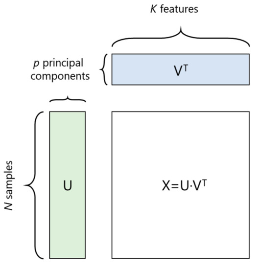
Figure 1.
Principal component method.
For PCA, we considered up to the third principal component, accounting for 79% of dataset variability as shown in the elbow chart (Figure 2). The method is based on the computation of the percentage of variance explained as a function of the principal component number. The trend of the curve in Figure 2 shows that the higher the number of components, the lower the marginal gain obtained by addition of another component.
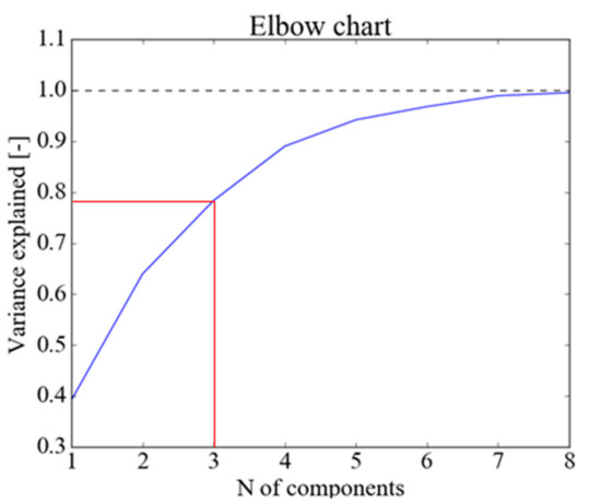
Figure 2.
Data-set variation vs. number of components.
2.2. Projection to Latent Structure
Projection to latent structure is a statistical method that acts on the data similarly to the PCA, with the main difference being that the features of the original dataset are grouped in input and output, and PLS aims to find relationships between these sub-sets. Specifically, PLS will find the multidimensional direction in the input variables space X that defines the maximum multidimensional variance in the output variables space Y [22]. In its general form, PLS creates orthogonal score vectors (also called latent vectors or components) by maximizing the covariance between these different sets of variables [9,23]. The influence of each input variable is quantified computing the loading vector for each considered component. Similar to the PCA loadings interpretation, highly correlated variables have similar weights in the loading vector. Different from PCA, PLS shows the influence exerted by the input variables on the selected outputs. Note that, before performing PLS analysis, all the variables have been normalized to avoid issues related to different variable units.
3. Dataset
The complete set of features considered for each individual are summarized in Table 1, which also shows how PCA considers all the features together, while PLS divides them into input and output features.

Table 1.
Features of fans inside the dataset, divided into input and output features according to projection to latent structures (PLS) analysis.
The dataset for PCA and PLS was populated considering three different families of industrial fans generated from three parent individuals labelled as Fan A, B, and C, Table 2. The families are labelled in the same way. The parent individuals were selected according to different segments of the fan market, considering the same original size and variations in hub-to-tip ratio, blade numbers, rotational speed, and design duty point. The geometry of each individual is completely defined, so it is possible to derive the chord and twist distributions of the blade, the pitch angle at the hub, and the 2D profile of the blade at different radii. Chord and twist distributions were characterized using the coefficients of a second order interpolating polynomial. Here, the factors that enter the analysis are C1, C2, T1, and T2, respectively, the linear and quadratic terms of the chord distribution, and those of twist distribution. To these we add C0, the chord at the hub, while T0 is neglected because twist at the hub is equal to 0. Admittedly a direct correlation with the work distribution along the blade span could be more accurate, yet data on the design of these fans are generally not available, especially since fans are usually operated in off-design conditions.
Table 2.
Parent individuals for of the dataset.
Starting from the three parent individuals, a population of three families with more than 1300 individuals per family was generated. The approach followed a process of scaling and cutting of different blades, to exploit one design to cover a wide operating envelope. In practice, it is possible to adjust the same design to a different fan size by scaling in similitude. Additionally, to extend the operating range and save in manufacturing process, the same blade can be cut at the tip to fit a higher hub-ratio. The possible variations of all the input parameters are summarized in Table 3. The performance of each fan was calculated using AxLab, an in-house axis-symmetric code [8]. All the information was stored inside a MySQL database and then processed through an in-house Python tool. Figure 3 and Figure 4 show the overall population of individuals, respectively, on the Q−ΔP plane and the Dtip−χ plane, which will be used for discussion of the results. The Q−ΔP plane shows the fan performance, and the Dtip−χ plane is related to the size of the device.
Table 3.
Characterization of the families of individuals for data analysis.
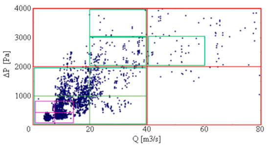
Figure 3.
Dataset population on Q−ΔP plane. Different boxes show the sub-set for data analysis.
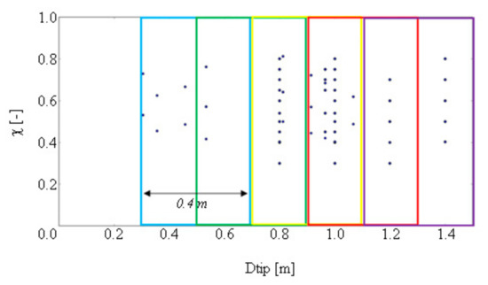
Figure 4.
Dataset population on size chart Dtip−χ. Different boxes show the sub-set for data analysis.
4. Results
Like all the statistical techniques used for data analysis, PCA and PLS can work on very large datasets and provide insights on the correlations between parameters of all the design space. Of course, this means that applying the analysis to all the data, results are likely to distillate general rules, valid on the whole design space. Since the possible application of this approach is to drive an optimization algorithm, it makes more sense to focus on correlations that apply to specific design sub-spaces. These can be identified in different ways, and here we decided to focus on the design point of the fan in terms of flow rate and pressure rise, and to the size of the fan, identified by the tip diameter and the hub-to-tip ratio. Then we went back to the respective charts, shown in Figure 3 and Figure 4, and here divided the design space in different sub-spaces with grids of different sizes and partially overlapping, to derive results linked to that specific subset. For example, here we report on analyses carried out for (i) fans operating at low flow-rate/low pressure-rise, (ii) fans operating at high flow-rate/high pressure-rise, and (iii) 0.3 m < Dtip < 0.7 m. On each sub-dataset we applied PCA to identify clusters of individuals with similar features. Then we carried out a PLS analysis on each sub-dataset to derive correlations between input and output features and derive design rules. A final summary of the rules derived from all the sub-dataset is given in the conclusions.
4.1. Q−ΔP Analysis
In Figure 5, the PCA score plots corresponding to the sub-sets of low flow rate–low pressure rise and high flow rate–high pressure rise are shown. The first plot is characterized by three clusters and as expected these can be directly linked to the three families of fans of the dataset. This is indirect proof of the capability of this approach to find correlations between sparse data. The second score plot in the same figure, with individuals working at high flow rates, shows two clusters of data, one with individuals from the A family, the other populated with fans belonging to the A and C families. In this case of extreme performance, a low number of individuals is present and therefore there is no direct link to the original families.
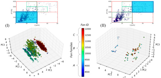
Figure 5.
Principal component analysis (PCA) score plots for the subset of individuals with low flow rate-low pressure rise (I) and high flow rate/high pressure rise (II) working conditions. Fan ID: number of individual.
From PLS analysis of individuals working at lower flow rates, Table 4, it follows that the first four latent variables have a strong correlation between input and output scores. This means that it is possible to find correlations between the loading coefficients of the original values in all the four latent variables, Figure 6. From the plot coefficient of LV1 we can see that there is a direct correlation between midspan solidity, chord at the hub (C0), and peak efficiency. As for chord and twist distributions, the increase of quadratic terms C2 and T2 has a direct correlation with the same peak efficiency, while there is an inverse proportionality between the linear terms C1 and T1. All the other loadings are lower than the threshold value (dashed red line) and therefore must be interpreted as not significant. Here, threshold values are calculated according to the correlation coefficient that refers to the observed latent component according to:
where LVi is the i-th latent component, wi and ci are the loadings of input and output features, and ti and ui are the scores of input and output features. CM is the correlation matrix between scores of input and output features.
Tr(LVi) = min (abs(wi,ci)) + [max (abs(wi,ci)) − min (abs(wi,ci))]∗[1 − CM(ti,ui)]
Table 4.
Correlations between latent variables.
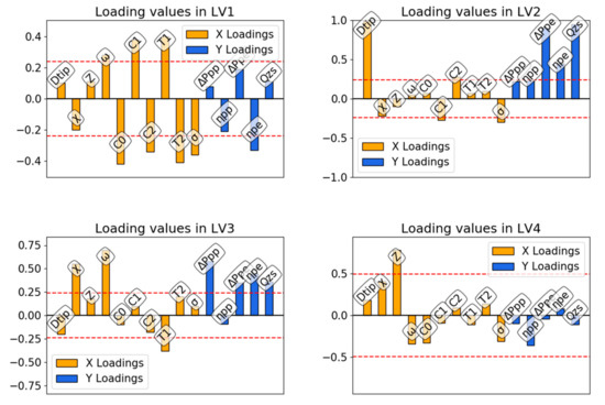
Figure 6.
PLS loadings for the subset of individuals (I) in Figure 5.
If we look at the coefficients for LV2 we can see that increasing Dtip leads to an increase of ΔPpe, ηpe, and Qzs: The whole stable range of operations shifts to higher flow rates and pressures. Loadings in LV3 show that an increase in χ and ω leads to increases of ΔPpp and ΔPpe and also in ηpe.
Basically, we can see that from the loadings of LV1, an increase in efficiency at peak efficiency can be achieved by changing the chord and twist distribution of the blade increasing C0, C2, and T2, while decreasing C1 and T1. Keeping C0 fixed to simplify, a fan increases in efficiency as the rotor twist and chord distributions are changed according to Figure 7.
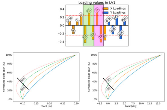
Figure 7.
LV1 PLS loadings for lower flow rates (top) and corresponding changes in chord (bottom left) and twist distributions (bottom right) that result in increase of efficiency at peak efficiency and peak pressure.
Computing the scores from the sub-dataset of fans working at high flow rates—high pressure ratio, Table 5, all these four latent variable loadings appear to be influential. The loading plots in Figure 8, however, suggest that the only relevant relationships between inputs X and output Y are explained by the third and fourth latent variables, as the loadings of outputs in the first two are below the threshold. In LV3, however, we can see that an increase in efficiencies at peak pressure and peak efficiency is achieved, increasing the rotational speed of the fan or decreasing the number of blades or the midspan solidity. The fact that in this case no clear indication is given about chord and twist distributions is probably to be related to the lower number of samples in this sub-dataset.
Table 5.
Correlations between latent variables.
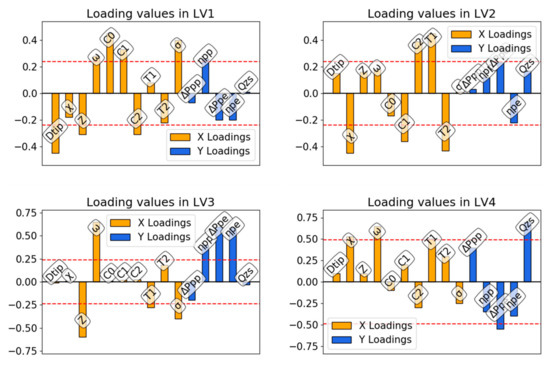
Figure 8.
PLS loadings for the subset of individuals (II) in Figure 5.
4.2. Dtip−χ Analysis
The same data processing can be applied selecting the fans according to their size, and here we focus on those fans that have Dtip between 0.3 m and 0.7 m. The PCA score plot, shown in Figure 9, highlights the presence of three clusters. One of them is clearly composed of fans belonging to the C family, while the other two include fans that belong to both A and B families. This kind of clustering seems to be related to the original rotating velocity of the fans, that for family C is half of that of families A and B. The low number of individuals in this dataset is reflected by the low level of correlations found in the PLS analysis, Table 6. In this case the loading plots, Figure 10, shows that for LV1 there is an inverse correlation between peak efficiency and rotational speed, a direct proportionality between peak efficiency and midspan solidity, and, in general, a strong correlation between peak efficiency and chord and twist distributions.
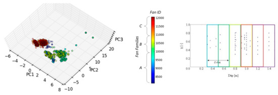
Figure 9.
PCA score plots for the subset of individuals with 0.3 m < Dtip < 0.7 m.
Table 6.
Correlations between latent variables.
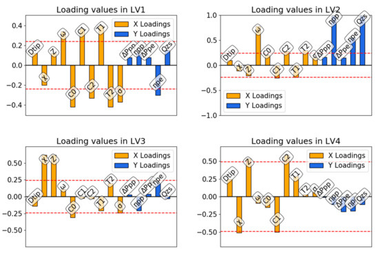
Figure 10.
PLS loadings for the subset of individuals with 0.3 m < Dtip < 0.7 m.
The second latent variable loadings show a direct proportionality of rotational velocity with efficiency at peak pressure and peak efficiency operations. The third and fourth latent variable loadings are not significant, as they are below threshold values.
5. Conclusions
Big Data Methods (PCA and PLS) were applied to a dataset of ~4000 individuals belonging to three fan families. The analysis was carried out on a series of sub-datasets corresponding to different ranges of fan performance and different fan sizes, aiming at discovering hidden correlations among design parameters and fan performance. Correlations already present in literature were found, as pressure increased alongside increases of blade number, confirming the validity of the method. Other findings emerged from a deeper analysis of PLS loadings.
As it was not possible to show all the relationships for all the sub-datasets analyzed, we summarize our findings in Figure 11, Figure 12, Figure 13 and Figure 14. In Figure 11 we summarized the relationship between midspan solidity and efficiency at peak pressure and peak efficiency in different regions of the Q−ΔP plane. In particular, the region in green, corresponding to low flow-rate/low pressure rise is characterized by a direct proportionality between σ and ηpp and ηpe. For individuals in the orange region the proportionality is limited to ηpp. Finally, in the blue region an inverse proportionality between σ and ηpe is found.
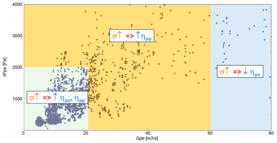
Figure 11.
PLS: Correlations of midspan solidity and fan efficiency according to the fan operating point.
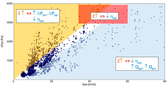
Figure 12.
PLS: Correlations of blade number and fan performance according to the fan operating point.
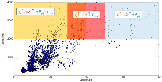
Figure 13.
PLS: Correlations of hub ratio, blade number, and fan performance according to the fan operating point.
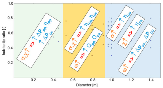
Figure 14.
PLS: Correlations of fan design parameters and fan performance according to the fan size.
In the same way, Figure 12 shows the relationships between blade number and different fan performance, for individuals belonging to different regions, while other relationships between design parameters and fan performance are presented in Figure 13. The same analysis, carried out on the size chart Dtip−χ led to results summarized in Figure 14.
Finally, the possible biases in the dataset must be highlighted: In fact, all the individuals originated from a process of scaling and cutting applied to three parent individuals. The fact that PCA highlights the presence of three clusters strongly related to the parent individuals, is indirect proof that the method works, but also that some relationships could be related to this generating mechanism. Furthermore, some sub-datasets used have a low number of individuals and it is possible that the low correlations that emerged from PLS were derived from an insufficient number of samples.
Author Contributions
Conceptualization, G.A., A.C., G.D. and L.T.; Data curation, G.A., A.C., G.D. and L.T.; Formal analysis, G.A., A.C., G.D. and L.T.; Investigation, G.A., A.C., G.D. and L.T.; Methodology, G.A., A.C., G.D. and L.T.; Software, G.A., A.C., G.D. and L.T.; Validation, G.A., A.C., G.D. and L.T. G; Visualization, G.A., A.C., G.D. and L.T.; Writing—original draft, G.D.; Writing—review & editing, A.D.
Funding
This research received no external funding.
Acknowledgments
The Authors would like to thank Giovanni Nardini who was instrumental in the first stage of this research.
Conflicts of Interest
The authors declare no conflict of interest.
References
- Cordier, O. Ahnlichkeitsbedingungen fur Stromungsmaschinen. BWK 1953, 5, 337–340. [Google Scholar]
- Wallis, R.A. Axial Flow Fans; George Newnes Ltd.: London, UK, 1961. [Google Scholar]
- Smith, S.F. A Simple Correlation of Turbine Efficiency. Aeronaut. J. 1965, 69, 467–470. [Google Scholar] [CrossRef]
- Balje, O.E. Turbomachines; John Wiley: New York, NY, USA, 1981. [Google Scholar]
- Howell, A.R. The Present Basis of Axial Flow Compressor Design; British Aeronautical Research Council: London, UK, 1942. [Google Scholar]
- Lieblein, S.; Schwenk, F.C.; Broderick, R.L. Diffusion Factor for Estimating Losses and Limiting Blade Loadings in Axial-Flow-Compressor Blade Elements; National Advisory Committee for Aeronautics: Washington, DC, USA, 1953.
- Bonanni, T.; Corsini, A.; Delibra, G.; Volponi, D.; Sheard, A.G. Derivative Design of Axial Fan Range: From Academia to Industry. In Proceedings of the ASME Turbo Expo 2016: Turbomachinery Technical Conference and Exposition, Seoul, Korea, 13–17 June 2016. [Google Scholar] [CrossRef]
- Bonanni, T.; Corsini, A.; Delibra, G.; Volponi, D. Design of a Single Stage Variable Pitch Axial Fan. In Proceedings of the ASME Turbo Expo, Charlotte, NC, USA, 26–30 June 2017. [Google Scholar]
- Rosipal, R.; Krämer, N. Overview and recent advances in partial least squares. In International Statistical and Optimization Perspectives Workshop “Subspace, Latent Structure and Feature Selection”; Springer: Berlin/Heidelberg, Germany, 2005; pp. 34–51. [Google Scholar]
- Erevelles, S.; Fukawa, N.; Swayne, L. Big Data consumer analytics and the transformation of marketing. J. Bus. Res. 2016, 69, 897–904. [Google Scholar] [CrossRef]
- Labrinidis, A.; Jagadish, H.V. Challenges and opportunities with big data. Proc. VLDB Endow. 2012, 5, 2032–2033. [Google Scholar] [CrossRef]
- Fan, J.; Han, F.; Liu, H. Challenges of big data analysis. Natl. Sci. Rev. 2014, 1, 293–314. [Google Scholar] [CrossRef] [PubMed]
- Lohr, S. The age of big data. New York Times, 11 February 2012. [Google Scholar]
- Kagaya, H.; Aizawa, K. Highly accurate food/non-food image classification based on a deep convolutional neural network. In Proceedings of the International Conference on Image Analysis and Processing, Genoa, Italy, 7–8 September 2015. [Google Scholar]
- Tam, K.Y.; Kiang, M. Predicting bank failures: A neural network approach. Appl. Artif. Intell. 1990, 4, 265–282. [Google Scholar] [CrossRef]
- Ahn, C.P.; Alexandroff, R.; Allende Prieto, C.; Anders, F.; Anderson, S.F.; Anderton, T.; Andrews, B.H.; Aubourg, E.; Bailey, S.; Bastien, F.A.; et al. The Tenth Data Release of the Sloan Digital Sky Survey: First Spectroscopic Data from the SDSS-III Apache Point Observatory Galactic Evolution Experiment. ApJS 2014, 211, 17. [Google Scholar] [CrossRef]
- Lintott, C.; Schawinski, K.; Bamford, S.; Slosar, A.; Land, K.; Thomas, D.; Edmondson, E.; Masters, K.; Nichol, R.C.; Raddick, M.J.; et al. Galaxy Zoo 1: Data release of morphological classifications for nearly 900 000 galaxies. Mon. Not. R. Astron. Soc. 2011, 410, 166–178. [Google Scholar] [CrossRef]
- Jagadish, H.V. Big data and science: Myths and reality. Big Data Res. 2015, 2, 49–52. [Google Scholar] [CrossRef]
- Mackiewicz, A.; Ratajczak, W. Principal components analysis (PCA). Comput. Geosci. 1993, 19, 303–342. [Google Scholar] [CrossRef]
- Abdi, H.; Williams, L.J. Principal Component Analysis; Wiley: Hoboken, NJ, USA, 2010; pp. 433–459. [Google Scholar]
- Svante, W.; Esbensen, K.; Geladi, P. Principal component analysis. In Chemometrics and Intelligent Laboratory Systems; Elsevier: Amsterdam, The Netherlands, 1987; Volume 2, pp. 37–52. [Google Scholar]
- Abdi, H. Partial Least Squares Regression and Projection on Latent Structure Regression (PLS Regression). In Wiley Interdisciplinary Reviews: Computational Statistics; Wiley: Hoboken, NJ, USA, 2010; Volume 2, pp. 97–106. [Google Scholar]
- Svante, W.; Sjöström, M.; Eriksonn, L. Partial least squares projections to latent structures (PLS) in chemistry. In Encyclopedia of Computational Chemistry; Von Ragué Schleyer, P., Allinger, N.L., Clark, T., Gasteiger, J., Kollman, P.A., Schreiner, P.R., Eds.; Wiley: Hoboken, NJ, USA, 2002. [CrossRef]
© 2019 by the authors. Licensee MDPI, Basel, Switzerland. This article is an open access article distributed under the terms and conditions of the Creative Commons Attribution (CC BY-NC-ND) license (https://creativecommons.org/licenses/by-nc-nd/4.0/).