Abstract
Despite the critical role of parking supply in urban transportation, the nonlinear relationship between parking facilities and commute mode choice remains poorly understood. This study systematically examines the nonlinear influences of the built environment, with a focus on parking facilities, on commuting mode choice using 2019 survey data from Xi’an. A Gradient Boosting Decision Tree (GBDT) model combined with Accumulated Local Effects (ALE) analysis was applied to capture complex relationships. The parking-related variables encompass factors such as parking fees, distance to the nearest parking lot, number of parking spaces, and parking density. Key findings indicate that car ownership, gender, land use mix-work, and distance to CBD-work, distance to CBD-home, and number of parking spaces-home at home are significant predictors. Notably, the number of parking spaces proved more influential than parking density. A positive correlation was observed between parking supply at workplaces and car usage, with a sharp increase in the probability of car ownership when supply exceeds 2800 spaces/km2. Similarly, a threshold of 7500 spaces/km2 around residences significantly promotes car dependence. The results underscore the importance of incorporating nonlinear parking supply effects into travel demand forecasting and provide insights for developing targeted parking management policies.
1. Introduction
Cars attract travelers because of their high efficiency and comfort. However, increasing dependence on cars has resulted in many negative impacts, such as carbon emissions, traffic congestion, and noise [1]. Consequently, scholars, planners, and local governments around the world are encouraging travelers to use public transit for commuting [2] in order to reduce commuter-generated carbon emissions (TCE) [3]. Commuters’ travel behaviour is strongly influenced by the built environment and demographics. Understanding the complex relationship between the built environment and residents’ commuting travel mode choices is crucial for optimizing mode split and alleviating urban traffic problems.
Parking availability is a pivotal built-environment attribute shaping travel mode decisions [4]. Adjustments to parking regulations-such as annual permit fees, hourly parking rates, the number of parking spaces, and parking lot locations-significantly influence the choice of bus transportation [5]. Regarding the impact of parking supply, numerous studies have demonstrated that scarce or inconvenient parking facilities and greater distances from destinations are key deterrents to driving among commuters, thereby reducing traffic congestion and air pollution [6]. However, research on the influence of parking facilities has typically relied on questionnaire data analyzing travelers’ mode preferences or Point of Interest (POI) data [7]. Crucially, actual parking lot attributes such as parking fee, the number of parking spaces, and the distance to the nearest parking lot have often been excluded, potentially introducing bias. Despite receiving limited scholarly attention, the potential for non-linear dynamics between parking-related factors and mode choice warrants a nuanced examination.
This study leverages 2019 travel survey data from Xi’an and employs a Gradient Boosting Decision Tree (GBDT) model. The primary objective is to scrutinize the influence of built environment and demographic characteristics, with a specific focus on parking-related factors, on commuting mode choice. The research framework is depicted in Figure 1, and the study is guided by the following research questions: (1) Which factors most significantly influence mode choice, and what are their relationships with mode choice? (2) How do parking facilities influence mode choice? (3) Do these parking facilities-related variables affect the model prediction accuracy, feature importance, and the relationships between the mode choice selection and explanatory variables?
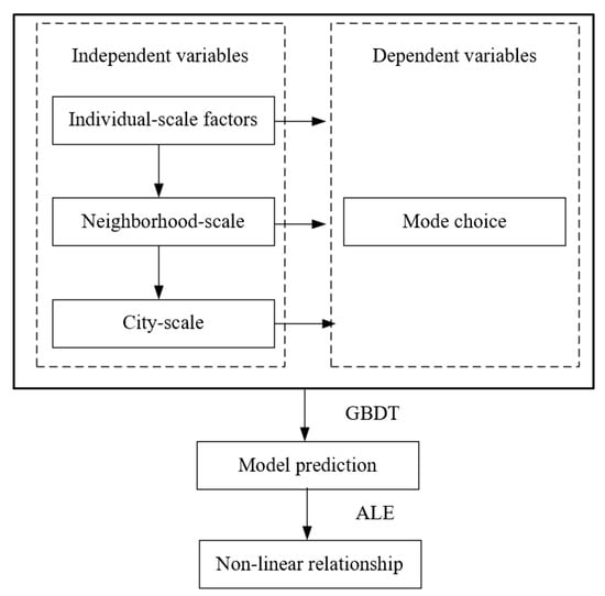
Figure 1.
Research framework.
The paper is structured as follows: Section 2 synthesizes the literature on mode choice influencers and analytical models, giving particular attention to parking facility attributes. Section 3 delineates the study area and data sources. The methodology and results are detailed in Section 4 and Section 5, respectively. Finally, Section 6 concludes with a summary of key findings and their policy implications.
2. Literature Review
Travel mode choice [8] and parking behavior [9] represent two critical dimensions of travel behavior. A body of literature has established that socio-demographic attributes—such as age, gender, income, education, and household registration (hukou)—are significant determinants of travel mode choice [10,11,12,13], built environment like land use mix, distance to CBD, bus stop density, metro station density, road network density, etc. [14,15,16], and accessibility [17]. Furthermore, A microeconomic behavioral modelling study by Frank et al. [18] identified residential and employment location and travel costs as the primary factors explaining mode choice differences. Higher population density, mixed land use, and pedestrian-friendly street design are negatively correlated with car reliance [19]; conversely, automobile ownership and underdeveloped public transit systems exhibit a positive correlation [20]. This fundamental dynamic continues to inform urban planning and transportation policy research [19,21].
Parking is a central determinant of travel demand, as it constitutes the start and end point of virtually all journeys [22]. Parking affects mode choice by influencing car ownership [23]. Parking also is the sixth “D” in “6D” [24] and “7D” [25], which evolved from the foundational “5D” theory [26]. Low-cost parking lots can increase car ownership [27,28], whereas reducing parking supply can reduce car ownership [29]. Number of parking lots [22], parking costs [30] and payment type [31], parking distance [32] and parking convenience [33], illegal parking fines [34], available parking spaces [35], parking control strategy [36] and parking fee increase [37] and other factors have been used to represent the parking behavior and intention of travelers obtained via the parking questionnaire under the SP survey or supply survey. These studies consistently identify a relationship between parking conditions and mode choice, demonstrating that parking availability influences travel behavior [38]. Guo demonstrated that restricted home parking availability effectively curbs household car use. While Rye et al. [39], illustrating through a case study in Edinburgh, confirmed that workplace parking restrictions within controlled zones significantly influence commuters’ mode choice away from private vehicles. Additionally, Point of Interest (POI) data for parking facilities [40,41,42] is frequently utilized. However, POI data only provides parking lots’ coordinates. While the parking fee and the number of parking spaces are also important characteristics that influence travelers’ parking behavior that remain understudied [43]. Insufficient attention to these actual parking facility characteristics hinders the development of appropriate parking supply planning strategies for achieving low-carbon transportation. Therefore, systematically understanding the parking demand’s impact mechanism is essential for promoting sustainable urban transportation development and improving quality of life. Moreover, critical questions regarding parking’s influence remain unresolved. Specifically, the non-linear relationship between parking provisions and mode choice is poorly understood. The research is also insufficient in verifying how parking facilities, such as the number of spaces, impact the accuracy of mode choice predictions, and in clarifying how parking availability at home and workplace distinctly shapes car ownership and usage patterns [44].
Conventional analytical paradigms in travel behavior research have long been dominated by statistical regression frameworks, most notably the discrete choice model, e.g., multinomial logit models, mixed logit models, and nested logit models. While these traditional methods offer strong theoretical foundations and interpretability, they rely on several unrealistic assumptions regarding data distribution, potentially leading to biased predictions. To overcome these limitations, machine learning (ML) methods have attracted researchers to use them for prediction and relationship analysis. Unlike statistical models, ML methods do not require strict assumptions about error distributions or functional forms linking predictors to responses. Instead, they enable computers to “learn” and identify complex patterns from large, noisy, or intricate datasets [45]. The selected algorithms include random forest (RF), support vector machine (SVM), artificial neural network (ANN), gradient boosting method (GBM), Extreme gradient boosting (XGBOOST), etc. [46,47]. The studies always focus on four primary travel modes: walking, cycling, public transit, and car, which constitute the core dependent variables for our analysis. The literature reflects a growing trend in applying machine learning techniques to travel behavior research, particularly for modeling and predicting mode choice. Among ML methods, GBDT has demonstrated superior prediction accuracy [45,48] and is widely used in travel behavior studies [49,50,51]. Despite their superior predictive performance, machine learning models face criticism for their “black box” nature and limited interpretability. This has spurred the development of techniques such as Partial Dependence Plots (PDP) and Accumulated Local Effects (ALE) plots to enhance model transparency [52]. The validity of Partial Dependence Plots (PDP) is contingent on a strict assumption of feature independence. However, in practical applications, this assumption is frequently violated due to inherent correlations among variables or measurement dependencies. To circumvent this limitation, Apley and Zhu (2016) [53] introduced Accumulated Local Effects (ALE) plots. This method calculates effects based on the conditional distribution of features, thereby yielding more reliable interpretations in the presence of correlated variables (For an extended discussion, see [54]). Although existing research has utilized machine learning to explore the non-linear relationships between the built environment and travel behavior, it exhibits several limitations, specifically regarding car usage. These include a scarcity of studies on this topic, a lack of investigation into the distinct effects of the built environment at trip origins and destinations, and a notable omission of parking supply, a factor highly correlated with car use. This study aims to elucidate the influence of parking availability, along with other built environment factors, on car usage patterns.
3. Data and Variables
3.1. Data Source
This study draws on two primary datasets from Xi’an: the 2019 regional household travel survey and a complementary parking lot survey, both provided by the Xi’an Urban Planning and Design Institute for urban infrastructure planning. Xi’an, located on the Guanzhong Plain in south-central Shaanxi Province (Figure 2), has a central urban area of approximately 766 square kilometers. As officially delineated in the Xi’an Territorial Space Master Plan (2021–2035) and depicted in Figure 3a, this area corresponds to the city’s core, comprising seven distinct administrative divisions. The average population densities for the seven districts are Xincheng: 2.0 × 10⁴, Beilin: 3.2 × 10⁴, Lianhu: 2.7 × 10⁴, Weiyang: 1.4 × 10⁴, Yanta: 1.9 × 10⁴, Baqiao: 0.9 × 10⁴ and Chang’an: 0.7 × 10⁴ people/km2.
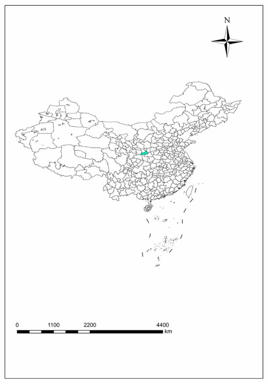
Figure 2.
The location of Xi’an city (blue area).
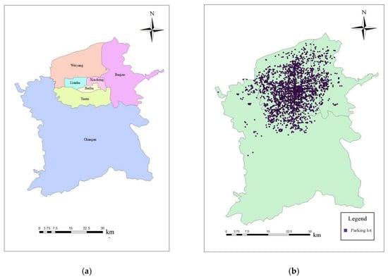
Figure 3.
Research area and parking lot distributions. (a) Research area. (b) Parking lots distribution.
The household travel survey captured individual socio-demographic attributes (e.g., age, gender, education), trip details (origin/destination coordinates, departure time), and car ownership. The complementary parking lot survey provided spatial locations, capacity, and pricing information for parking facilities, with their distribution illustrated in Figure 3b.
After removing the intercity records and cleaning the data, 27,081 trips were used for this research.
3.2. Description of Variables
A Gradient Boosting Decision Tree (GBDT) model was developed to examine the influence of built environment and demographic factors on commuting mode choice, with a specific focus on parking characteristics. Given the intrinsic link between car use and parking availability, the dependent variable-commuting mode-was categorized as either car or other (encompassing bus, metro, walking, cycling, and taxi). In the dataset, car mode accounted for 15.22% of the observed commutes.
The independent variables are measured by the separation between work and home. Data on population density are taken from Worldpop (https://hub.worldpop.org/). While a land use entropy index was computed based on fourteen functional types. Metrics for intersection density, bus stop density, metro station density, and distance to the CBD were obtained from 2019 OpenStreetMap data. Finally, parking-related variables (density, capacity, and proximity) were calculated in ArcGIS 10.8 using the parking lot survey data.
Table 1 is the descriptive statistical results of variables used in this research.

Table 1.
Descriptive profile of the variables.
4. Methodology
4.1. Model Selection
The influence of built environment and demographic factors on travel behavior is increasingly recognized as non-linear in nature. This complexity motivates the use of Gradient Boosting Decision Trees (GBDT), a method renowned for its high predictive accuracy and inherent capacity to capture such non-linear associations between mode choice and its predictors.
4.2. Mathematical Model
Gradient Boosting Decision Tree (GBDT) operates by iteratively combining weak learners, specifically Classification and Regression Tree (CART) models, into a strong ensemble model. It employs forward stage-wise additive modeling, where each new CART learner is fitted to the negative gradient (steepest descent) of the loss function from the previous iteration, effectively minimizing the residual error [45]. The Gini impurity criterion is used for node splitting within each CART, with lower values indicating higher node purity. The additive model is constructed greedily as shown in Equation (1).
where are weak learners (DTs); is the newly added tree that tries to minimize the loss function L; is the previous model; is step length.
The steepest descent direction is defined as the negative functional gradient of the loss function with respect to the current model, as formalized in Equation (3).
Step length is chosen using line search, as Equation (4) shows.
4.3. Model Interpretability
The GBDT model possesses intrinsic interpretability, primarily derived from its additive structure and the transparency of the boosting procedure [22]. Feature importance refers to how important features are in the model. If a feature is very important, it will greatly impact the model’s predictive performance. The Accumulated Local Effects (ALE) plot is designed to isolate and visualize the marginal effect of an explanatory variable on the model’s predicted outcome.
5. Results and Analysis
This paper presents a GBDT model trained in Python 3.11.1. The dataset was partitioned into a training set (80%) and a test set (20%). A grid search coupled with 5-fold cross-validation was then performed to identify the optimal hyperparameter combination. The optimal hyperparameters were found to be learning_rate = 0.1, n_trees = 100, and max_depth = 5.
The F1 score is a comprehensive metric that balances precision and recall, providing a single measure of a binary classification model’s accuracy. For more information, see Li and Kockelman (2022) [45]. The F1 score of the model is 0.87. Removing the parking-related variables, the model’s F1 score is 0.86. This suggests that the parking-related variables have little influence on the model’s predictions. With the demographic-related variables removed, the model’s F1-score decreased to 0.79. Table 2 displays the prediction performance of the three models across various metrics, including accuracy, precision, F1-score, recall, and AUC.

Table 2.
Relative contributions of independent variables on TCE.
In a Gradient Boosting Machine (GBM), the relative importance of a predictor is computed by aggregating the weighted reduction in the loss function resulting from every split on that variable across the entire ensemble of trees, with the final sum normalized to a percentage. The value ranges from 0 to 1, indicating the proportional contribution of that variable to the explanatory power of the model. A higher relative importance value indicates that the feature plays a more critical role in the model. The relative importance of all the variables is shown in Figure 4a. The feature importance of variables excluding the eight parking-related variables is shown in Figure 4b. Table 3 presents the relative predictive importance of the independent variables for car commuting in model 1.
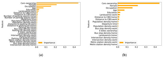
Figure 4.
Relative importance rank. (a) Model 1. (b) Model 2.

Table 3.
Relative contributions of independent variables on model choice (Model 1).
The analysis revealed that car ownership emerged as the predominant factor influencing mode choice, exerting the strongest influence, followed by gender (female) and occupation. This finding aligns with established research on the primary determinants of travel behavior [55,56]. Ding et al. pointed out that car ownership emerged as the dominant socio-demographic factor influencing travel mode choice [55]. Several built environment attributes were identified as pivotal in influencing travel mode choice. These included land use mix at workplace and distance to the CBD at workplace and at home, and the number of parking spaces at home and at workplace. The relative importance of the number of parking spaces is higher than the parking lot density, confirming the necessity to use the number of parking spaces in analyzing travel mode choice.
Using the Accumulated Local Effects (ALE) plots within the Gradient Boosted Decision Tree (GBDT) framework, commuters were categorized into car and non-car groups. This approach facilitated a detailed analysis of the non-linear associations between mode choice and key factors spanning the built environment and individual traveler characteristics. Figure 3 illustrates the influence of demographic characteristics on commute mode choice. As depicted in Figure 5a, car ownership demonstrates the strongest positive correlation with car usage. Figure 5b indicates a higher propensity for car commuting among males, while Figure 5c shows that business/service employees and freelancers exhibit a greater preference for car travel. A stronger inclination toward car use is also observed in the 41–69 age cohort (Figure 5d) and among individuals with higher educational attainment (Figure 5e).
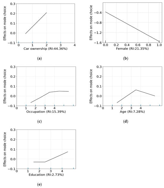
Figure 5.
ALE plots between demographics and mode choice (Model 1). (a) Car ownership. (b) Female, (c) Occupation, (d) Age, (e) Education.
Figure 6 illustrates the relationship between the number of parking spaces and mode choice, which exhibits a pronounced non-linear trend. Other parking-related variables are not displayed as their ALE plots displayed near-linear relationships, offering less interpretive value.
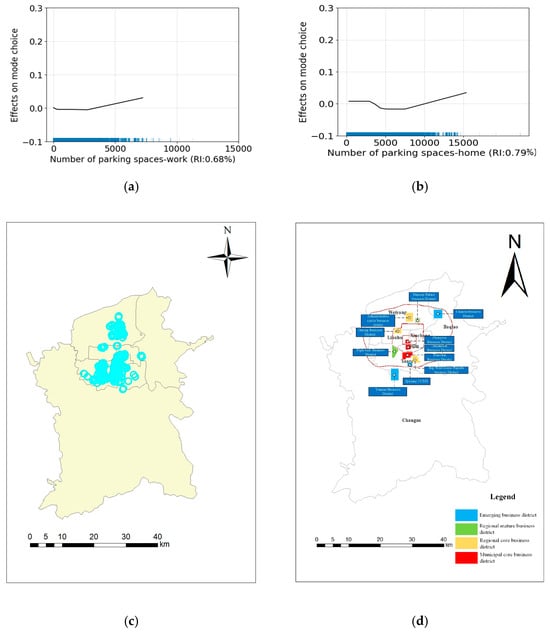
Figure 6.
ALE plots between parking-related variables and mode choice (Model 1). (a) Number of parking spcaes-work, (b) Number of parking spcaes-home, (c) Spatial correspondence between areas with a parking supply exceeding 7500 spaces/km2, (d) Major commercial zones. Note: The blue color indicates the frequency density of the independent variable, where greater density corresponds to a higher frequency.
The number of parking spaces at the workplace is positively correlated with mode choice (Figure 6a). If it is less than 2800 spaces/km2, there is no obvious change in mode choice. However, when it exceeds 2800 spaces/km2, its effect increases significantly. The ALE plot for the number of home parking spaces reveals a four-phase pattern, indicating distinct phases of influence on mode choice as availability increases (Figure 6b). When it is less than 3000 spaces/km2, there is no obvious variation in mode choice. As it increases from 3000 spaces/km2 to 4400 spaces/km2, the probability of choosing to commute by car decreases. The reason may be that it is close to the CBD, where parking fees are extremely high, and parking spaces are scarce, while the walking environment and public transportation are relatively convenient. When it increases from 4400 spaces/km2 to 7500 spaces/km2, the effect is minimal. When it exceeds 7500 spaces/km2. The increase in parking supply offset the impact of improved public transport accessibility. Commuters will be more inclined to use them. However, an increase in parking spaces will encourage more people to commute by car. A modal balance typically exists between public transport attractiveness and parking convenience. However, when parking supply surpasses a threshold of approximately 7500 spaces/km2, this balance is disrupted. Beyond this point, the abundance of parking significantly enhances the appeal of car commuting, leading to a higher propensity for car use. This observation aligns with findings by Guo et al, who confirmed the substantial influence of home-area parking availability on car ownership decisions. Our analysis also revealed a spatial correspondence between areas with a parking supply exceeding 7500 spaces/km2 (Figure 6c) and major commercial zones (Figure 6d). Higher-income groups, who tend to reside in these commercial areas, exhibit a stronger preference for car travel.
Figure 5 depicts the influence of key built environment variables on mode choice. Population density at both home and workplace exhibits a negative correlation with car use (Figure 7a,b). Notably, a threshold effect is observed: when densities remain below approximately 4800 persons/km2 (workplace) and 6600 persons/km2 (home), their influence is pronounced, beyond which their marginal effect diminishes significantly. This suggests that intensifying density has a strong payoff for reducing car dependence up to a point, after which further increases yield minimal additional benefits-a finding crucial for defining effective density-based policies.
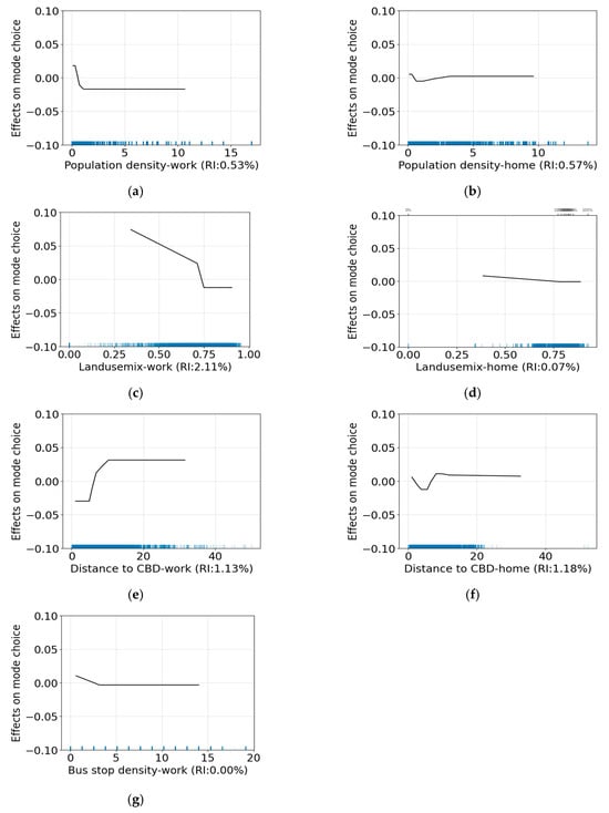
Figure 7.
ALE plots between belt-environment variables and mode choice (Model 1). (a) Population density-work, (b) Population density-home, (c) Land use mix-work, (d) Land use mix-home, (e) Distance to CBD-work, (f) Distance to CBD-home, (g) Bus stop density-work.
A negative correlation exists between land use mix and car travel choice (Figure 7c,d). For the workplace land use mix, a saturation threshold is observed at 0.75. Below this value, indicative of areas transitioning from single-use to moderately mixed functions, each increment in mix diversity substantially reduces car reliance. Beyond 0.75, representing well-established, highly mixed-use districts, the effect plateaus. This pattern implies that achieving a “good” level of land-use mix is sufficient to curb car use, with perfection offering little extra advantage—a key insight for prioritizing planning resources.
The influence of distance to the CBD on car commuting differs by location (Figure 7e,f). For the workplace, a pronounced positive correlation is observed. The threshold is 11 km. For the home location, the relationship is more complex and can be divided into three distinct segments: when the distance is below 2.8 km, it negatively correlates with car use. The possible reason for the slight decline might be that it is close to the city’s CBD, and the public transportation system is relatively complete. Between 2.8 km and 6.67 km, it tends to stabilize. Between 6.67 km and 10.26 km, the propensity for car travel increases with distance; beyond 10.26 km, the effect plateaus, indicating a saturation point. The distances from the CBD to the eastern, southern, western, and northern sides of the Second Ring Road are 11.5 km, 14.2 km, 8 km, and 11.7 km, respectively. Consequently, distance exerts a strong influence on travel mode choice within the Second Ring Road. Beyond this boundary, its effect diminishes markedly as individual preferences and other factors become more dominant.
Bus stop density at the workplace has a negative relationship with mode choice (Figure 7g). The threshold is 3 stops/km2. There are small relationship with the metro stop density because the metro in Xi’an was still under development in 2019.
Upon removal of the influential demographic factors, the ranking of variable importance is shown in Table 4 below.

Table 4.
Relative contributions of independent variables on mode choice (Model 3).
A comparison between Table 4 (Model 3) and Table 3 (Model 1) shows that removing demographic variables has little impact on the importance ranking of built environment variables, but their importance values increase. Key variables such as distance to CBD, population density, land use mix-work, and number of parking spaces-work remain highly influential.
Figure 8 illustrates the nonlinear relationships between some key variables and car usage. While the ALE plots of some variables show minor fluctuations, others, such as the number of parking spaces and distance to CBD, exhibit a clear linear increasing trend once the confounding effects of demographic variables are removed.
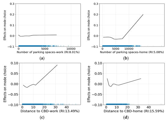
Figure 8.
ALE plots between belt-environment variables and mode choice (Model 3). (a) Number of parking spaces-work, (b) Number of parking spaces-home, (c) Distance to CBD-home, (d) Distance to CBD-work.
Compared to the ALE plot of Model 1, the curves for the number of parking spaces and distance to the CBD in Model 3 exhibit a clear upward trend as their values increase. This occurs because, in Model 1, the inclusion of demographic variables (such as age, gender, and car ownership) introduces a strong stratification effect on travel mode choice. Higher-income households and car owners show a greater tendency to use cars regardless of location, which masks or alters the true underlying relationship between distance/parking availability and car usage.
In contrast, after removing these demographic variables in Model 3, only built environment variables remain. This allows the direct influence of factors like job-housing separation, transportation supply, and parking conditions to be more clearly observed. As the distance to the city center increases, heightened job-housing separation reduces reliance on public transport for commutes. Simultaneously, suburban built environments, characterized by sparse public transit, wider roads, and ample parking, objectively encourage car use, whereas city centers suppress it through dense road networks, convenient public transit, and high parking costs. Consequently, the monotonically increasing relationship driven by the built environment—“the farther from the city center, the higher the tendency to use a car”—becomes clearly visible.
6. Conclusions
This study used Xi’an city as a case study, applying the GBDT method to investigate the relative importance of demographic and built environment variables, particularly parking—related variables, on mode choice, as well as their non-linear relationships. The findings contribute to the existing literature in several significant aspects.
First, the study demonstrates the non-linear relationship between explanatory variables and mode choice. While earlier studies have used machine learning techniques like GBDT to capture non-linear effects of the built environment, most have focused on general travel behavior rather than car use specifically. Our results not only reinforce the presence of such complex relationships but also quantify specific thresholds for key variables that lead to notable reductions in car dependency. Distance to the CBD–home and workplace are two important variables influencing car use. There is a lack of public transport facilities in the suburbs, so people tend to use cars for commuting. The land use mix at the workplace is also an important factor influencing mode choice. Urban planners should pay more attention to land use planning; diversified land types could significantly reduce car use, and the specific thresholds identified in this research (at least above 0.75) can be used as a reference point. This provides a more actionable insight for urban planners compared to earlier qualitative descriptions.
Secondly, it shows that the number of parking spaces is a more important predictor of mode choice than parking lot density, with a higher relative importance rank. Our findings highlight the distinct role of parking supply measures. While many previous studies emphasized parking lot density, this research demonstrates that the absolute number of parking spaces exerts a stronger influence on mode choice. The number of parking spaces in excess of 2800 spaces/km2 at workplaces and 7500 spaces/km2 at homes will have a significant impact on car usage. The greater the number of parking spaces, the more attractive car commuting becomes, so commuters are more inclined to choose the car. There is a balance between the influence of the attractiveness of public transport and the convenience of parking. In order to control the entry of cars and increase traffic congestion in urban areas, parking supply will be regulated. Meanwhile, the urban area has a well-developed public transportation system. As a result, the number of car trips decreases. However, when the threshold is exceeded, the balance between parking convenience and the convenience of public transportation trips is disrupted, and the choice of car trips increases sharply. Urban planners need to improve the public transport supply near residential areas and increase its attractiveness, in order to reduce parking demand. The number of parking spaces is more important than parking lot density, which confirms the need to consider the number of parking spaces when analysing mode choice. These variables do have an impact on the travel mode choice and cannot be ignored. This result aligns with, but importantly differentiates from, the former work, which found density-based metrics to be moderately influential. Our study suggests that overlooking the actual count of spaces may lead to an underestimation of parking’s impact, offering a more precise variable for future modeling and policy-making.
Finally, this study acknowledges its limitations, particularly its focus on commuting trips. Future research should incorporate diverse travel purposes and integrate on-street parking data to enhance the comprehensiveness and accuracy of parking supply representation. Expanding the application of the GBDT approach to other cities would also help validate the generalizability of the non-linear patterns and thresholds identified herein.
Author Contributions
Conceptualization, W.L.; methodology, W.L. and X.M.; software, X.M.; validation, W.L. and X.M.; formal analysis, Y.Z.; investigation, W.L. and Q.L.; resources, W.L.; data curation, X.M.; writing—original draft preparation, W.L., X.M., X.J. and B.T.; writing—review and editing, W.L. and Q.L.; visualization, W.L.; supervision, W.L. and Q.L.; project administration, W.L.; funding acquisition, W.L. All authors have read and agreed to the published version of the manuscript.
Funding
The authors gratefully acknowledge financial support from the Education Department of Shaanxi Provincial Government (item no.: 22JE004).
Institutional Review Board Statement
Not applicable.
Informed Consent Statement
Not applicable.
Data Availability Statement
The data that support the findings of this study are derived from a third party and are subject to restrictions under a confidentiality agreement. Therefore, they are not publicly available. However, data can be made available by the corresponding author upon reasonable request and with the permission of the third party.
Conflicts of Interest
Author Qiang Li and Binfeng Tuo were employed by the company Northwest Engineering Corporation Limited. The remaining authors declare that the research was conducted in the absence of any commercial or financial relationships that could be construed as a potential conflict of interest.
References
- Cao, J.; Ermagun, A. Influences of LRT on travel behaviour: A retrospective study on movers in Minneapolis. Urban Study 2016, 54, 2504–2520. [Google Scholar] [CrossRef]
- Boarnet, M.G.; Wang, X.; Houston, D. Can new light rail reduce personal vehicle carbon emissions? a before-after, experimental-control evaluation in Los Angeles. J. Reg. Sci. 2017, 57, 523–539. [Google Scholar] [CrossRef]
- Liu, W.; Pang, S.; Li, W.; Han, Y. Assessing the CO2 emission reduction potential of metro-bus combined travel through interpretable machine learning. Transp. A Transp. Sci. 2025, 1–24. [Google Scholar] [CrossRef]
- Ali, M. A machine learning approach to study the effect of parking pricing on transport mode choice to work using 2022 NHTS dataset. Case Stud. Transp. Policy 2025, 20, 101478. [Google Scholar] [CrossRef]
- Rotaris, L.; Danielis, R. The impact of transportation demand management policies on commuting to college facilities: A case study at the University of Trieste Italy. Transp. Res. Part A-Policy Pract. 2014, 67, 127–140. [Google Scholar] [CrossRef]
- Xiao, L.L.; Liu, T.L.; Huang, H.J. On the morning commute problem with carpooling behavior under parking space constraint. Transp. Res. Part B Methodol. 2016, 91, 383–407. [Google Scholar] [CrossRef]
- Liu, B.; Li, F.; Hou, Y.; Biancardo, S.A.; Ma, X.L. Unveiling built environment impacts on traffic CO2 emissions using Geo-CNN weighted regression. Transp. Res. Part D Transp. Environ. 2024, 132, 104266. [Google Scholar] [CrossRef]
- Tu, M.T.; Li, W.X.; Orfila, O.; Li, Y.; Gruyer, D. Exploring nonlinear effects of the built environment on ridesplitting: Evidence from Chengdu. Transp. Res. Part D Transp. Environ. 2021, 93, 102776. [Google Scholar] [CrossRef]
- Meng, F.Y.; Du, Y.C.; Li, Y.C.; Wong, S.C. Modeling heterogeneous parking choice behavior on university campuses. Transp. Plan. Technol. 2018, 41, 154–169. [Google Scholar] [CrossRef]
- De Vos, J.; Mokhtarian, P.L.; Schwanen, T.; Van Acker, V.; Witlox, F. Travel Mode Choice and Travel Satisfaction: Bridging the Gap between Decision Utility and Experienced Utility. Transportation 2016, 43, 771–796. [Google Scholar] [CrossRef]
- Cheng, L.; Chen, X.; Yang, S.; Wu, J.; Yang, M. Structural Equation Models to Analyze Activity Participation, Trip Generation, and Mode Choice of Low-Income Commuters. Transp. Lett. 2019, 11, 341–349. [Google Scholar] [CrossRef]
- Fang, J.; Yan, X.; Tao, T.; Chen, C.J. Non-linear effects of built environment factors on mode choice: A tour-based analysis. J. Transp. Land Use 2024, 17, 215–239. [Google Scholar] [CrossRef]
- Liu, Y.; Tang, R.; Shi, Z.B.; He, M.W.; Cheng, L. Shared mobility choices in metro connectivity: Shared bikes versus shared e-bikes. Transportation 2025, 52, 2187–2213. [Google Scholar] [CrossRef]
- Ding, C.; Wang, D.; Liu, C.; Zhang, Y.; Yang, J. Exploring the Influence of Built Environment on Travel Mode Choice Considering the Mediating Effects of Car Ownership and Travel Distance. Transp. Res. Part A-Policy Pract. 2017, 100, 65–80. [Google Scholar] [CrossRef]
- Ye, R.; Titheridge, H. Satisfaction with the Commute: The Role of Travel Mode Choice, Built Environment and Attitudes. Transp. Res. Part D Transp. Environ. 2017, 52, 535–547. [Google Scholar] [CrossRef]
- De Gruyter, C.; Saghapour, T.; Ma, L.; Dodson, J. How does the built environment affect transit use by train, tram and bus? J. Transp. Land Use 2020, 13, 625–650. [Google Scholar] [CrossRef]
- Huang, R. Simulating individual work trips for transit-facilitated accessibility study. Environ. Plan. B Urban Anal. City Sci. 2017, 46, 84–102. [Google Scholar] [CrossRef]
- Frank, L.; Bradley, M.; Kavage, S.; Chapman, J.; Lawton, T.K. Urban form, travel time, and cost relationships with tour complexity and mode choice. Transportation 2008, 35, 37–54. [Google Scholar] [CrossRef]
- Sun, B.; Ermagun, A.; Dan, B. Built environmental impacts on commuting mode choice and distance: Evidence from Shanghai. Transp. Res. Part D Transp. Environ. 2017, 52, 441–453. [Google Scholar] [CrossRef]
- Yang, J.; Kato, H.; Ando, R.; Nishihori, Y. Analyzing household vehicle ownership in the Japanese local city: Case study in toyota city. J. Adv. Transp. 2020, 2020, 7264860. [Google Scholar] [CrossRef]
- Tennøy, A.; Gundersen, F.; Øksenholt, K.V. Urban structure and sustainable modes’ competitiveness in small and medium-sized Norwegian cities. Transp. Res. Part D Transp. Environ. 2022, 105, 103225. [Google Scholar] [CrossRef]
- Chen, J.; Liu, K.L.; Di, J.; Peng, T. Nonlinear model of impact of built environment on urban parking demand. J. Transp. Syst. Eng. Inf. Technol. 2021, 21, 197–203. [Google Scholar]
- Guo, Z. Home parking convenience, household car usage, and implications to residential parking policies. Transp. Policy 2013, 29, 97–106. [Google Scholar] [CrossRef]
- Ao, Y.B.; Chen, C.; Yang, D.J.; Wang, Y. Relationship between Rural Built Environment and Household Vehicle Ownership: An Empirical Analysis in Rural Sichuan, China. Sustainability 2018, 10, 1566. [Google Scholar] [CrossRef]
- Wang, Z.B.; Song, J.R.; Zhang, Y.; Li, S.H.; Jia, J.L.; Song, C.C. Spatial Heterogeneity Analysis for Influencing Factors of Outbound Ridership of Subway Stations Considering the Optimal Scale Range of “7D” Built Environments. Sustainability 2022, 14, 16314. [Google Scholar] [CrossRef]
- Ewing, R.; Cervero, R. Travel and the built environment, A Meta-Analysis. J. Am. Plan. Assoc. 2010, 76, 265–294. [Google Scholar] [CrossRef]
- Guo, Z. Does residential parking supply affect household car ownership? The case of New York City. J. Transp. Geogr. 2013, 26, 18–28. [Google Scholar] [CrossRef]
- Tyrinopoulos, Y.; Antoniou, C. Factors affecting modal choice in urban mobility. Eur. Transp. Res. Rev. 2013, 5, 27–39. [Google Scholar] [CrossRef]
- Chatman, D.G. Deconstructing development density: Quality, quantity and price effects on household non-work travel. Transp. Res. Part A-Policy Pract. 2008, 42, 1008–1030. [Google Scholar] [CrossRef]
- Yang, C.; Ho, Y. Assessing carbon reduction effects toward the mode shift of green transportation system. J. Adv. Transp. 2016, 50, 669–682. [Google Scholar] [CrossRef]
- Pimenta, A.; Kamruzzaman, L.; Huda, F.; Currie, G. Examining parking preferences with private autonomous vehicles using random forest and logit models: The case of commuters to central Melbourne. Res. Transp. Econ. 2025, 114, 101651. [Google Scholar] [CrossRef]
- Christiansen, P.; Engebretsen, Ø.; Fearnley, N.; Hanssen, J.U. Parking facilities and the built environment: Impacts on travel behaviour. Transp. Res. Part A-Policy Pract. 2017, 95, 198–206. [Google Scholar] [CrossRef]
- Scheffler, T.; Klockner, C.A.; Heinen, E. Where I live is what I do—The potential of residential choices to determine energy use and travel behaviour of Norwegian movers. Travel Behav. Soc. 2026, 42, 101138. [Google Scholar] [CrossRef]
- Xue, Y.; Cheng, L.; Lin, P.; An, J.; Guan, H. Parking space reservation behavior of car travelers from the perspective of bounded rationality: A case study of nanchang city, China. J. Adv. Transp. 2020, 2020, 8851372. [Google Scholar] [CrossRef]
- Djakfar, L.; Bria, M.; Wicaksono, A. How Employees Choose their Commuting Transport Mode: Analysis Using the Stimulus-Organism-Response Model. J. Adv. Transp. 2021, 2021, 5555488. [Google Scholar] [CrossRef]
- Pan, S.L.; Zheng, G.J.; Chen, Q. The psychological decision-making process model of non-commuting travel mode choice under parking constraints. Transp. Res. Interdiscip. Perspect. 2021, 11, 100410. [Google Scholar] [CrossRef]
- Peng, T.; Chen, J.; Liu, K.L.; Qiu, Z.X.; Fu, Z.Y.; Huang, Y. Examining the relationship between built environment and urban parking demand from the perspective of travelers. J. Clean. Prod. 2023, 385, 135766. [Google Scholar] [CrossRef]
- Ma, X.L.; Yang, J.; Ding, C.; Liu, J.F.; Zhu, Q. Joint Analysis of the Commuting Departure Time and Travel Mode Choice: Role of the Built Environment. J. Adv. Transp. 2018, 2018, 4540832. [Google Scholar] [CrossRef]
- Rye, T.; Cowan, T.; Ison, S. Expansion of a Controlled Parking Zone (CPZ) and its Influence on Modal Split: The Case of Edinburgh. Transp. Plan. Technol. 2006, 29, 75–89. [Google Scholar] [CrossRef]
- Yin, C.Y.; Shao, C.F.; Wang, X.Q. Built Environment and Parking Availability: Impacts on Car Ownership and Use. Sustainability 2018, 10, 2285. [Google Scholar] [CrossRef]
- Liu, K.L.; Chen, J.; Li, R.; Peng, T.; Ji, K.K.; Gao, Y.Y. Nonlinear Effects of Community Built Environment on Car Usage Behavior: A Machine Learning Approach. Sustainability 2022, 14, 6722. [Google Scholar] [CrossRef]
- Xi, Y.F.; Hou, Q.H.; Duan, Y.Q.; Lei, K.X.; Wu, Y.; Cheng, Q.Y. Exploring the Spatiotemporal Effects of the Built Environment on the Nonlinear Impacts of Metro Ridership. ISPRS Int. J. Geo-Inf. 2024, 13, 105. [Google Scholar] [CrossRef]
- Kim, E.J. Analysis of Travel Mode Choice in Seoul Using an Interpretable Machine Learning Approach. J. Adv. Transp. 2021, 2021, 6685004. [Google Scholar] [CrossRef]
- Christiansen, P.; Fearnley, N.; Hanssen, J.U.; Skollerud, K. Household parking facilities: Relationship to travel behaviour and car ownership. Transp. Res. Procedia 2017, 25, 4185–4195. [Google Scholar] [CrossRef]
- Li, W.J.; Kockelman, K. How does machine learning compare to conventional econometrics for transport data sets? A test of ML versus MLE. Growth Change 2021, 53, 342–376. [Google Scholar] [CrossRef]
- Chang, X.M.; Wu, J.J.; Liu, H.; Yan, X.Y.; Sun, H.J.; Qu, Y.C. Travel Mode Choice: A Data Fusion Model Using Machine Learning Methods and Evidence from Travel Diary Survey Data. Transp. A Transp. Sci. 2019, 15, 1587–1612. [Google Scholar] [CrossRef]
- Wang, S.H.; Mo, B.C.; Zheng, Y.H.; Hess, S.; Zhao, J.H. Comparing Hundreds of Machine Learning Classifiers and Discrete Choice Models in Predicting Travel Behavior: An Empirical Benchmark. Transp. Res. Part B Methodol. 2024, 190, 103061. [Google Scholar] [CrossRef]
- Sun, Y.L.; Dong, Y.N.; Waygood, E.O.; Naseri, H.; Jiang, Y.H.; Chen, Y.J. Machine-Learning Approaches to Identify Travel Modes Using Smartphone-Assisted Survey and Map Application Programming Interface. Transp. Res. Rec. 2022, 2677, 385–400. [Google Scholar] [CrossRef]
- Zhang, W.J.; Zhao, Y.J.; Cao, X.Y.; Lu, D.M.; Chai, Y.W. Nonlinear effect of accessibility on car ownership in Beijing: Pedestrian-scale neighborhood planning. Transp. Res. Part D Transp. Environ. 2022, 86, 102445. [Google Scholar] [CrossRef]
- Shao, Q.F.; Zhang, W.J.; Cao, X.Y.; Yang, J.W. Built environment interventions for emission mitigation: A machine learning analysis of travel-related CO2 in a developing city. J. Transp. Geogr. 2023, 110, 103632. [Google Scholar] [CrossRef]
- Tong, D.; Bierlaire, M.; Dai, Y.; Shen, Y. Commuting behaviors response to living and working built environment: Dissecting interaction effects from varied supply and demand masses. Appl. Geogr. 2024, 172, 103430. [Google Scholar] [CrossRef]
- Kashifi, M.T.; Jamal, A.; Kashefi, M.S.; Almoshaogeh, M.; Rahman, S.M. Predicting the travel mode choice with interpretable machine learning techniques: A comparative study. Travel Behav. Soc. 2022, 29, 279–296. [Google Scholar] [CrossRef]
- Apley, D.W.; Zhu, J.Y. Visualizing the Effects of Predictor Variables in Black Box Supervised Learning Models. J. R. Stat. Soc. Ser. B Stat. Methodol. 2020, 82, 1059–1086. [Google Scholar] [CrossRef]
- Molnar, C. Interpretable Machine Learning. 2020. Available online: https://christophm.github.io/interpretable-ml-book/ (accessed on 3 December 2025).
- Ding, C.; Wang, Y.P.; Tang, T.Q.; Mishra, S.; Liu, C. Joint analysis of the spatial impacts of built environment on car ownership and travel mode choice. Transp. Res. Part D Transp. Environ. 2018, 60, 28–40. [Google Scholar] [CrossRef]
- Haque, M.B.; Choudhury, C.; Hess, S.; dit Sourd, R.C. Modelling residential mobility decision and its impact on car ownership and travel mode. Travel Behav. Soc. 2019, 17, 104–119. [Google Scholar] [CrossRef]
Disclaimer/Publisher’s Note: The statements, opinions and data contained in all publications are solely those of the individual author(s) and contributor(s) and not of MDPI and/or the editor(s). MDPI and/or the editor(s) disclaim responsibility for any injury to people or property resulting from any ideas, methods, instructions or products referred to in the content. |
© 2026 by the authors. Licensee MDPI, Basel, Switzerland. This article is an open access article distributed under the terms and conditions of the Creative Commons Attribution (CC BY) license.