Prediction of Rail Wear Under Different Railway Track Geometries Using Artificial Neural Networks

Abstract

The geometry of the railway track affects rail wear significantly. If the rail wear can be predicted and considered during the alignment design phase, the problems it causes can be mitigated at the source by optimizing the values and combinations of railway track geometry parameters. However, the relationship between railway track geometry and rail wear remains unclear. It is hard to acquire rail wear data for different alignments with varying geometric parameters during the alignment design phase. This study develops a PSO-ANN model to establish the mapping relationship between railway track geometry and rail wear, enabling prediction of rail wear based on track geometry parameters. The model achieves prediction accuracies of 96.70% for inner rail wear and 98.13% for outer rail wear. Compared with the conventional ANN model, the PSO-ANN model reduces the prediction errors by 22.54% for inner rail wear and 55.69% for outer rail wear. Sobol sensitivity analysis is conducted to analyze the influence of the track geometry parameters on rail wear, revealing that inner rail wear is mainly affected by curve radius, transition curve length, and superelevation, while outer rail wear is predominantly influenced by curve radius.

1. Introduction

Rail wear is a critical issue for railway infrastructure. The costs of rail maintenance and replacements due to rail/wheel wear reach billions of CNY (China Yuan) annually in China [1]. The material loss in the rail alters the rail profile, which changes the location of wheel contact points and compromises vehicle stability, particularly during curving. This deteriorates the train’s running stability and, more seriously, can cause train derailments. Track geometry is one of the most significant factors influencing rail wear, especially in curved sections [2]. Therefore, if rail wear can be predicted and considered during the alignment design phase, the problems it causes can be mitigated at the source by optimizing track geometry parameters.

For the studies about rail wear calculation, numerical models are widely used. Many scholars established multibody dynamics models and finite element models to calculate the rail wear. Ignesti et al. [3] developed a 3D multibody model of a railway vehicle using the commercial software SIMPACK, incorporating a contact model between the wheel and rail to calculate the forces at the contact patches. These contact forces were then fed into a wear model implemented in the MATLAB environment to calculate rail wear. Li et al. [4], from Singapore, employed the commercial software Universal Mechanism (UM) to calculate the rail wear using the modified expression of Archard’s law. The influences of vehicle speed, curve radius, and superelevation on the rail wear are analyzed. Li et al. [5] introduced a numerical method to simulate rail profile wear and applied it to a heavy-haul line in China. Their approach integrates three key models: A coupled freight vehicle-track dynamics model, a non-Hertzian contact model, and a material wear model to compute wear evolution. The effectiveness of rail wear calculation methods based on numerical models has been demonstrated in numerous studies [6,7,8]. However, the modeling process is complex, and the simulations are time-consuming. During the railway alignment design phase, multiple alignment alternatives need to be designed for comparison and analysis. Establishing numerical models for each alternative and calculating rail wear through simulations is highly time-consuming, significantly reducing design efficiency and making the design time unacceptable.

Significant reductions in computational time can be achieved by predefining relationships between influential parameters and rail wear. These relationships are derived from comprehensive numerical experiments spanning diverse scenarios, with regression analysis employed to develop surrogate models that approximate the input-output relationships [9]. Yin et al. [10] established three kinds of surrogate models based on the response surface method (RSM), support vector machine (SVM), and relative vector machine (RVM) to predict the rail wear. The wheel-rail friction coefficient, curve radius, axle load, superelevation, and vehicle suspension coefficient are considered. Zhou [11] developed a surrogate model based on a T-S fuzzy neural network to predict rail wear, considering factors such as train speed, curve radius, rail bottom slope, and axle load. The artificial neural networks (ANNs) were employed by Wang et al. [12] to establish a surrogate model to predict rail wear, which takes train speed, axle load, and wheel-rail impact angle as input data.

The aforementioned approaches improve the efficiency of rail wear acquisition by establishing surrogate models that consider multiple influencing parameters. However, track geometry parameters are not adequately considered, with only a few factors, such as curve radius, typically included. Track geometry is determined by various parameters, including both horizontal track parameters (i.e., curve radius, circular curve length, transition curve length, and superelevation) and vertical track parameters (i.e., gradient and gradient algebraic difference). Variations in these parameters and their combinations alter the track geometry [13,14], which in turn affects the rail wear. Therefore, it is essential to consider these track geometry parameters and establish their relationship with the rail wear, enabling accurate predictions of rail wear under different track geometries.

This study focuses on the impacts of railway track geometry on rail wear and develops a surrogate model to predict rail wear based on track geometry parameters, including curve radius, circular curve length, transition curve length, superelevation, gradient, and gradient algebraic differences. A PSO-ANN model, combining particle swarm optimization (PSO) with an artificial neural network (ANN), is proposed to establish the mapping relationship between railway track geometry and rail wear. Additionally, Sobol analysis is conducted to assess the sensitivities of track geometry parameters on the rail wear. The outline of this paper is as follows: Section 2 presents the numerical models used for calculating rail wear. Section 3 details the PSO-improved ANN (PSO-ANN) proposed in this study for rail wear prediction. Section 4 offers the results of numerical experiments and discussions. Finally, Section 5 summarizes the work in this study.

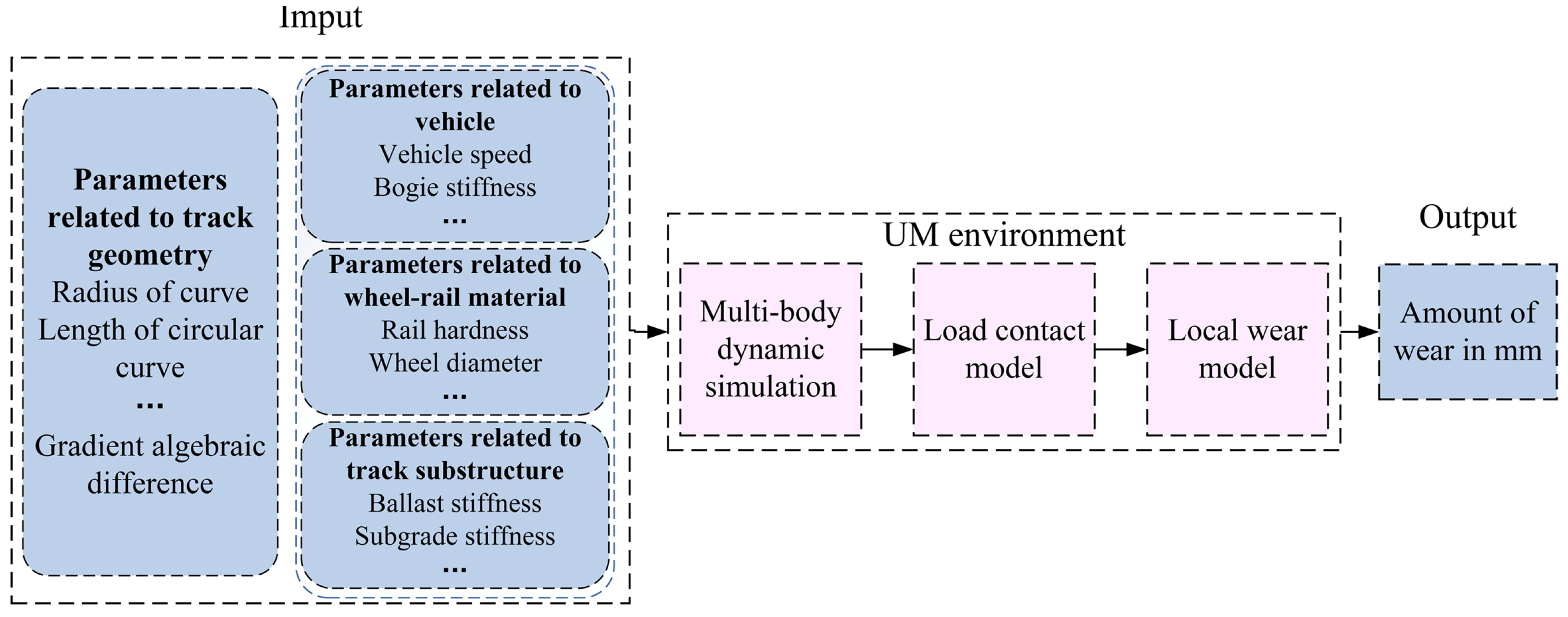
2. Rail Wear Calculation

Rail wear is calculated through a multibody dynamics model (i.e., a vehicle-track coupling model) and a wear model, as shown in Figure 1. Different combinations of input parameters are fed into the multibody dynamics model. Through dynamic simulations, the wheel-rail contact parameters are generated and then fed into the wear model to yield the amount of wear area loss. The multibody dynamic model and the wear model are introduced in the following subsections.

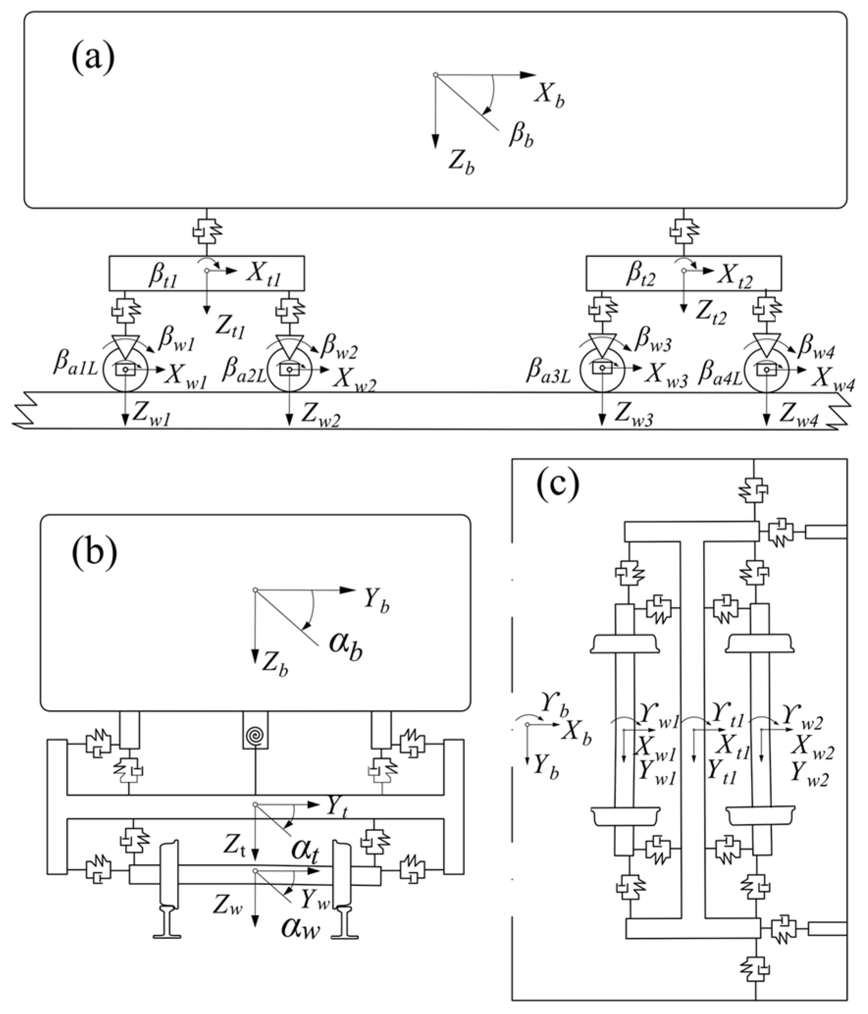
2.1. Multibody Dynamic Model

The multibody dynamic simulations are performed in UM in this study. The Metro Type A vehicle is selected as the prototype to establish a vehicle model, which consists of one car body and two bogies. Each bogie is made up of one frame, two wheelsets, and four axle boxes. The frame is connected by two suspensions, and the wheelset and the frame are connected by one suspension. Figure 2 shows the structure of the vehicle model. The entire vehicle model has a total of 50 degrees of freedom [15]. The car body, frame, and wheelsets consider six degrees of freedom, which are expansion (car body X_b, bogie X_t1, X_t2, wheelset X_w1, X_w2, X_w3, X_w4), nodding (car body β_b, bogie β_t1, β_t2, wheelset β_w1, β_w2, β_w3, β_w4), shaking (car body γ_b, bogie γ_t1, γ_t2, wheelset γ_w1, γ_w2, γ_w3, γ_w4), rolling (car body α_b, bogie α_t1, α_t2, wheelset α_w1, α_w2, α_w3, α_w4), lateral shift (car body Y_b, bogie Y_t1, Y_t2, wheelset Y_w1, Y_w2, Y_w3, Y_w4), and sinking (car body Z_b, bogie Z_t1, Z_t2, wheelset Z_w1, Z_w2, Z_w3, Z_w4). The axle box considers only nodding β_i (i = 1L, 1R, …, 4L, 4R). Detailed parameters of the vehicle model can be found in Lei et al. [16], as shown in

Table 1. Main vehicle parameters.

Parameters	Values
Frame mass (kg)	4420
Vehicle mass (kg)	26,040
Length of vehicle (m)	22.0
Width of vehicle (m)	3.0
Wheel-base bogie (m)	2.5
Vehicle spacing (m)	15.7
Moment of inertia of body pitching (kg·m2)	1.1 × 106
Moment of inertia of bogie pitching (kg·m2)	4902
The primary spring vertical damping (Ns/m)	2400
The secondary spring vertical damping (Ns/m)	23,000
vehicle speed (km/h)	60

.

The track model is established by configuring track geometry parameters, such as curve radius, curve length, transition curve length, superelevation, gradient, and gradient algebraic difference. The CHN60 rail type is adopted. The material parameters for the wheel and rail are listed in

Table 2. Main mechanical properties of wheel and rail materials.

Wheel-Rail Materials	Tensile Strength/MPa	Yield Strength/MPa	Brinell Hardness/HB
Rail	880~950	460~530	260~300
Wheel	800~860	400~480	270~300

, with the wheel–rail friction coefficient set to 0.35. The track model includes rail movement degrees of freedom in the lateral and vertical directions, as well as rotational freedom in the longitudinal direction.

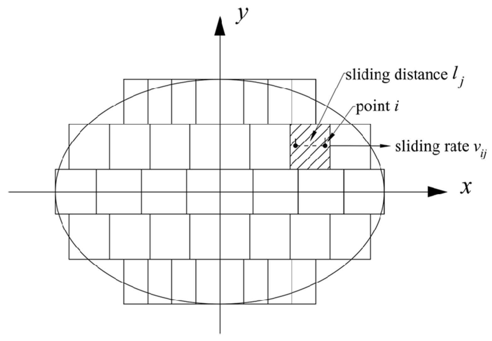
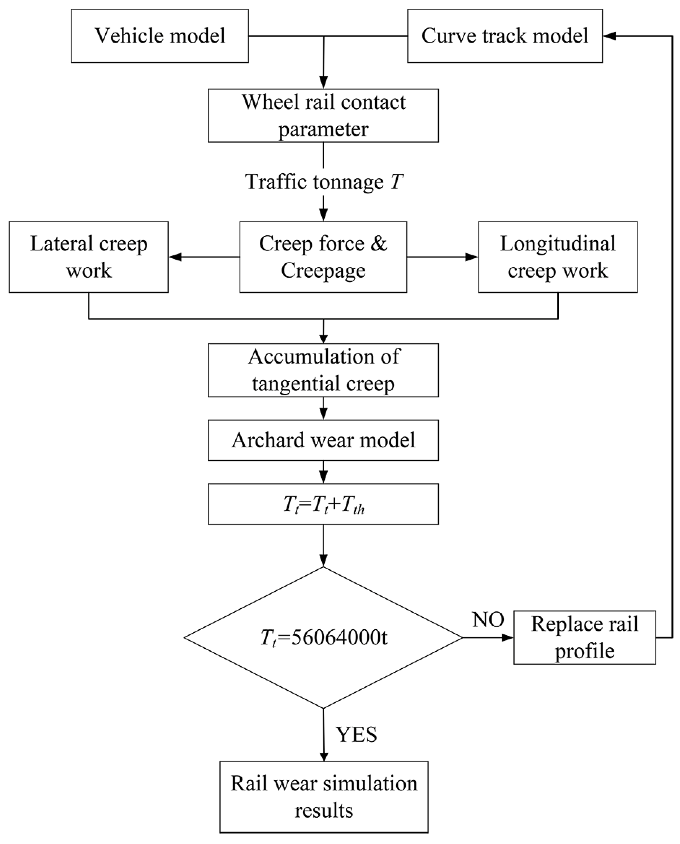
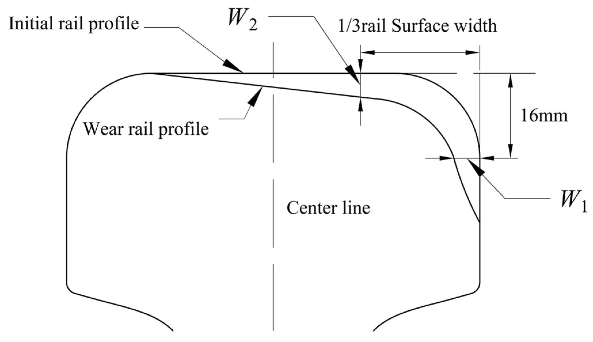
2.2. Rail Wear Model

Rail wear calculation is an iterative and reciprocating process. Firstly, the wheel-rail contact parameters (e.g., contact point positions, contact forces, creepages, etc.) are generated through the dynamic simulation. Based on this, the rail wear at the wheel-rail contact spot is calculated and the rail profile is updated. The updated rail profile is then incorporated into the multibody dynamic model for the next iteration, where rail wear is recalculated and a wear rail profile is obtained.

Material volume loss caused by rail wear can be categorized into distinct mechanisms, including abrasive, adhesive, corrosive, and surface fatigue wear [18]. Among these, adhesive wear is the predominant mechanism in wheel-rail contact scenarios [19]. Consequently, this study employs an adhesive wear model derived from Archard’s law [20], expressed by the original formula:

$$V_{wear}=k{\displaystyle \frac{N\cdot s}{H}}$$

(1)

where V_wear is the wear volume of the material (m³); k is the wear index, which is decided by the material of contact body; N is the normal contact force (N); s is the sliding distance; and H is the surface hardness of the softer material (N/m²). As evidenced in Equation (1), V_wear is proportional to N and s and inversely proportional to H. In the case where the friction coefficient μ is constant, Equation (1) reduces to

$$V_{wear}=k_m{W}_s$$

(2)

$$k_m={\displaystyle \frac{k}{H\cdot \mu }},W_s=\mu \cdot N\cdot s$$

(3)

where W_s represents the sliding work of the friction forces obtained by the wheel-rail contact and k_m is the corrected wear empirical index obtained through testing.

Due to creep dominating the state of the wheel-rail contact on the curved section, the sliding work should be calculated according to the creep force. The tangential creep force F_ij at any point i on the contact spot can be calculated by Equation (4):

$$F_{ij}=f(N_{ij},{\xi }_{ij})$$

(4)

where N_ij represents the point normal force on the contact spot and ξ_ij represents the wheel-rail creepage; in this context, j represents the directions in the lateral and longitudinal axes (j = x, j = y).

Under different creep conditions, the relationship between wheel-rail creep force and wheel-rail creepage is not constant. Under conditions of small creep, the wheel-rail creep force is linearly related to the wheel-rail contact through a constant creep coefficient ξ_ij. However, as creep increases, this relationship becomes nonlinear, indicating that the creepage is not uniform across every point within the contact patch. Therefore, this study employs the Kik-Piotrowski contact model to analyze the wheel-rail contact relationships [21,22]. The model assumes a semi-elliptical normal pressure distribution along the rolling direction. The contact area is determined by the virtual penetration of the wheel and rail. Normal pressure is calculated by meeting the contact conditions at the geometric contact point, while the tangential contact force is determined using an improved FASTSIM algorithm. In this algorithm, the contact patch is discretized into equal-width strips parallel to the x-axis, which are further divided into equal numbers of elements, as shown in Figure 3. The sliding distance l_j is obtained by integrating the sliding rate v_sj over time in each direction j, as shown in Equation (5). And the work W_sij due to creep in direction j at the point is calculated with Equation (6).

$$l_j={\displaystyle \int v_{sj}}dt$$

(5)

$$W_{sij}=F_{ij}{l}_j=f(N_{ij},{\xi }_{ij}){\displaystyle \int v_{sj}}dt$$

(6)

Based on the theoretical analysis above, calculating rail wear volume at the rail contact spot requires integrating Equation (6) over the contact area. However, as each contact point on the rail can be treated as a microcell, the creep displacement at each microcell is minimal as the wheel passes, and the area of each microcell is very small relative to the wear value. Therefore, the wear volume can be approximated by the wear value at each individual point.

Figure 4 shows the simulation flowchart for rail wear calculation used in this study. It is assumed that each track section serves for 10 years, with 40 trains passing daily. Each train consists of six formations. The total number of train passes can be converted into gross traffic tonnage, yielding 3.504 × 10⁶ wheelset passes, equivalent to a cumulative load of 56,064,000 tons (i.e., T_t = 56,064,000 t). To calculate rail wear, the progressive change in rail profile at each iteration is considered. A threshold value, T_th (where T_th = 140,160 t), is set in the calculation. When the traffic tonnage reaches this threshold, the rail profile is updated for the next iteration step, and this process continues until the cumulative gross traffic tonnage reaches 56,064,000 t.

After the rail wear simulation, the final worn rail profile is obtained. According to the national standards in China [23,24], rail wear (W_t) is composed of two components: side rail wear (W₁) and vertical rail wear (W₂). The measurement methods for vertical and side rail wear are illustrated in Figure 5. The vertical wear is measured at 1/3 of the rail surface width of the rail (from the standard working edge), and the side wear is measured at 16 mm below the rail tread. After measuring the side and vertical rail wear, the rail wear can be calculated with Equation (7):

$$W_t={\displaystyle \frac{1}{2}}{W}_1+W_2$$

(7)

where W_t is the rail wear (mm); W₁ is the lateral rail wear (mm); and W₂ is the vertical rail wear (mm).

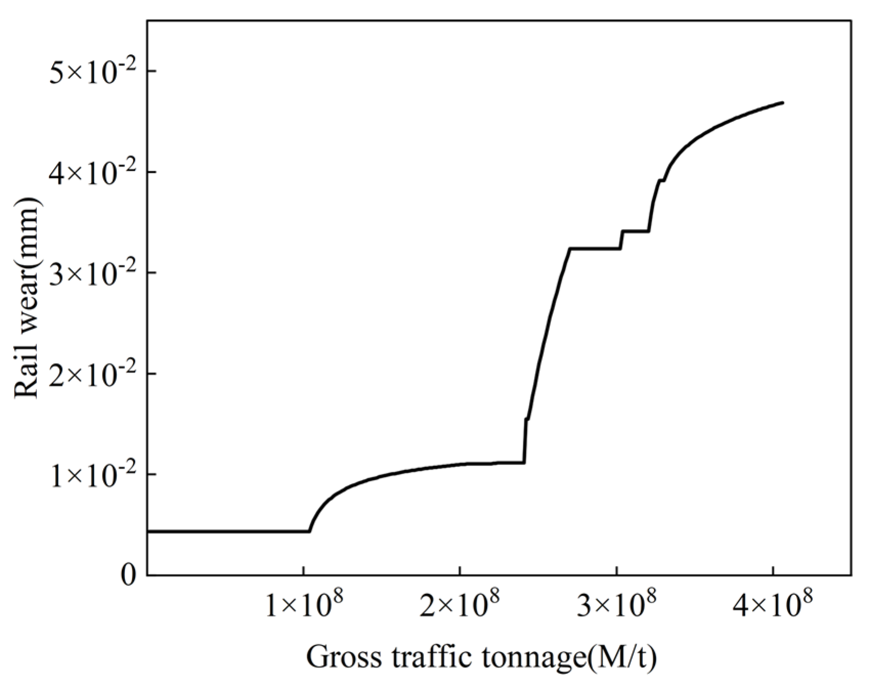
2.3. Model Verification

In order to verify the calculation accuracy of the rail wear using the above method, the rail side wear of a real-world railway measured by Lei et al. [16] is introduced. The parameters of the multi-body dynamic model and rail wear model are set according to the real-world railway in literature, of which the wheel tread and rail profile are wheel LMA and rail CHN60 of China Railway, the friction coefficient between the wheel and rail is 0.35, the vehicle axle load is 14 t, the vehicle speed is 60 km/h, the transition curve length is 140 m, the circular curve length is 200 m, the curve radius is 400 m, the rail bottom slope is 1/40, the wheel passing times is 2.9 × 10⁷, and the gross traffic tonnage is 4.06 × 10⁸ t. The simulation results are shown in Figure 6.

According to Figure 6, it can be seen that the rail wear through model simulation is 0.04687 mm, while the corresponding real-world measured rail wear is 0.04900 mm. The difference between the simulation and measured rail wear is only 0.00213 mm, which demonstrates the effectiveness of the simulation model.

3. Artificial Neural Networks for Rail Wear Prediction

Railway track geometry affects the rail wear dramatically. The primary goal of this study is to substitute the computationally intensive process between the input and output in Figure 1 with artificial neural networks, enabling efficient evaluation of a wide range of track geometries and thereby enhancing the quality of railway alignment design.

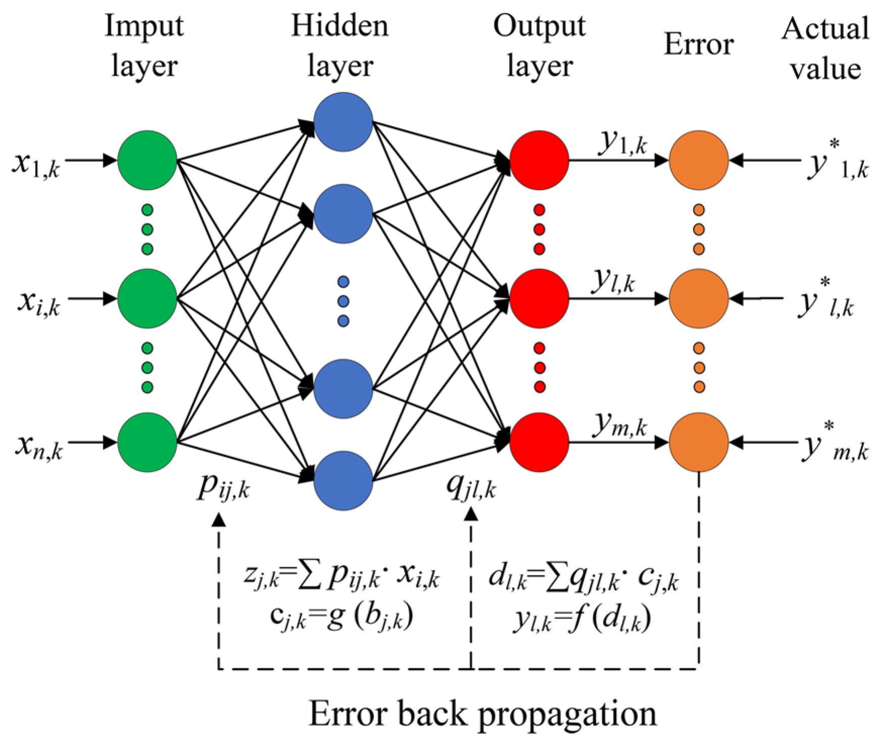
3.1. Artificial Neural Network (ANN)

Artificial neural networks (ANNs) are widely used to solve complex engineering problems. It can learn from samples, making it highly useful for simulating correlations that are difficult to describe using physical models or other mathematical expressions [25]. As a multilayer feedforward neural network trained through error back propagation, ANN possesses strong self-organizing learning capabilities. With suitable network parameters, it can accurately express various nonlinear relationships.

Within a feedforward neural network, information flows from the network’s inputs to its outputs. Figure 7 shows a feedforward neural network model with the input layer, output layer, and one hidden layer, where z_j,k and c_j,k are the input and output of the jth node in the hidden layer, and d_l,k and y_l,k are the input and output of the lth node in the output layer. For the establishment of ANN models, the primary task is to determine the network topology and experimental data processing. According to Hornik et al. [26], a three-layer ANN model, which has one hidden layer, can approximate any function to any precision. Therefore, one hidden layer is applied in this study, and in order to eliminate the difference in order of magnitude between input and output data and avoid causing a large prediction error, the data are normalized. The normalization process is as follows:

$$x^{\prime }={\displaystyle \frac{x-x_{\min }}{x_{\max }-x_{\min }}}$$

(8)

where x′ is the normalized data; x is the original data; x_min and x_max are the minimum and maximum values of x, respectively.

For the hidden layer, the number of nodes affects the model performance dramatically. An excessive number of nodes may cause the model to overfit, while too few nodes may result in predictions that fall short of requirements. Normally, the number of nodes is determined based on experience and experiments. In this study, an empirical formula (Equation (9)) from Liu et al. [27] is introduced, according to which the number of nodes in the hidden layer is determined through the trial-and-error method based on the training data. Detailed experiments are provided in Section 4.1.

$$h=\sqrt{m+n}+a$$

(9)

where h is the number of nodes in the hidden layer; n is the number of nodes in the input layer; m is the number of nodes of the output layer; a is an arbitrary constant between 1 and 10.

The Levenberg–Marquardt learning algorithm [28] is applied to update the weights (i.e., p_ij,k and q_jl,k) of the ANN models, as shown in Equations (10) and (11).

$$\begin{gathered} \left[\begin{array}{c}{p}_{ij,k+1}\\ q_{jl,k+1}\end{array}\right]=\left[\begin{array}{c}{p}_{ij,k}\\ q_{jl,k}\end{array}\right]-{\left[H_k+\alpha I\right]}^{-1}\left[\begin{array}{c}{\displaystyle \frac{\partial E_k}{\partial p_{ij,k}}}\\ {\displaystyle \frac{\partial E_k}{\partial q_{jl,k}}}\end{array}\right] \\ {H}_k=\left[\begin{array}{cc}{\displaystyle \sum _{ijl}\frac{{\partial }^2{E}_k}{\partial p_{ij,k}^2}}& {\displaystyle \sum _{ijl}\frac{{\partial }^2{E}_k}{\partial p_{ij,k}\partial q_{jl,k}}}\\ {\displaystyle \sum _{ijl}\frac{{\partial }^2{E}_k}{\partial p_{ij,k}\partial q_{jl,k}}}& {\displaystyle \sum _{ijl}\frac{{\partial }^2{E}_k}{\partial q_{ij,k}^2}}\end{array}\right],{\displaystyle \sum _{ijl}=}{\displaystyle \sum _i{\displaystyle \sum _j{\displaystyle \sum _l}}} \end{gathered}$$

(10)

where p_ij,k are the weights of the hidden layer; q_jl,k are the weights of the output layer; H_k is the second derivative of E_k; E_k is the error function as shown in Equation (11); α is the learning factor; I is the unit matrix; i is the number of nodes in input layer (1 ≤ i ≤ n); j is the number of nodes in hidden layer; l is the number of nodes in output layer (1 ≤ l ≤ m); and k is the iteration. The error function is shown in Equation (11).

$$E_k={\displaystyle \frac{1}{2}}{\displaystyle \sum _{l=1}^m{({y^{*}}_l-y_l)}^2}$$

(11)

where $y_l^{*}$ is the true value; y_l is the output value of the ANN model.

The accuracy of the ANN models is influenced by the transfer function. According to the analysis results from Wang et al. [29], for predicting rail wear, the sigmoid function demonstrates clear advantages over other transfer functions, such as the Sin function. Therefore, this study employs the sigmoid function as the transfer function, as shown in Equation (12).

$$g(x)={\displaystyle \frac{1}{1+e^{-x}}}$$

(12)

The quality of the ANN model is assessed by the mean absolute percentage error (MAPE) [30] using a separate set of samples, which is calculated with Equation (13).

$$MAPE={\displaystyle \sum _{d=1}^D\frac{\left|y_d^{*}-y_d\right|}{y_d^{*}}}\times 100\%$$

(13)

where $y_d^{*}$ is the observed value of rail wear (through dynamic simulations); y_d is the predicted value of rail wear by the ANN model; D is the number of samples.

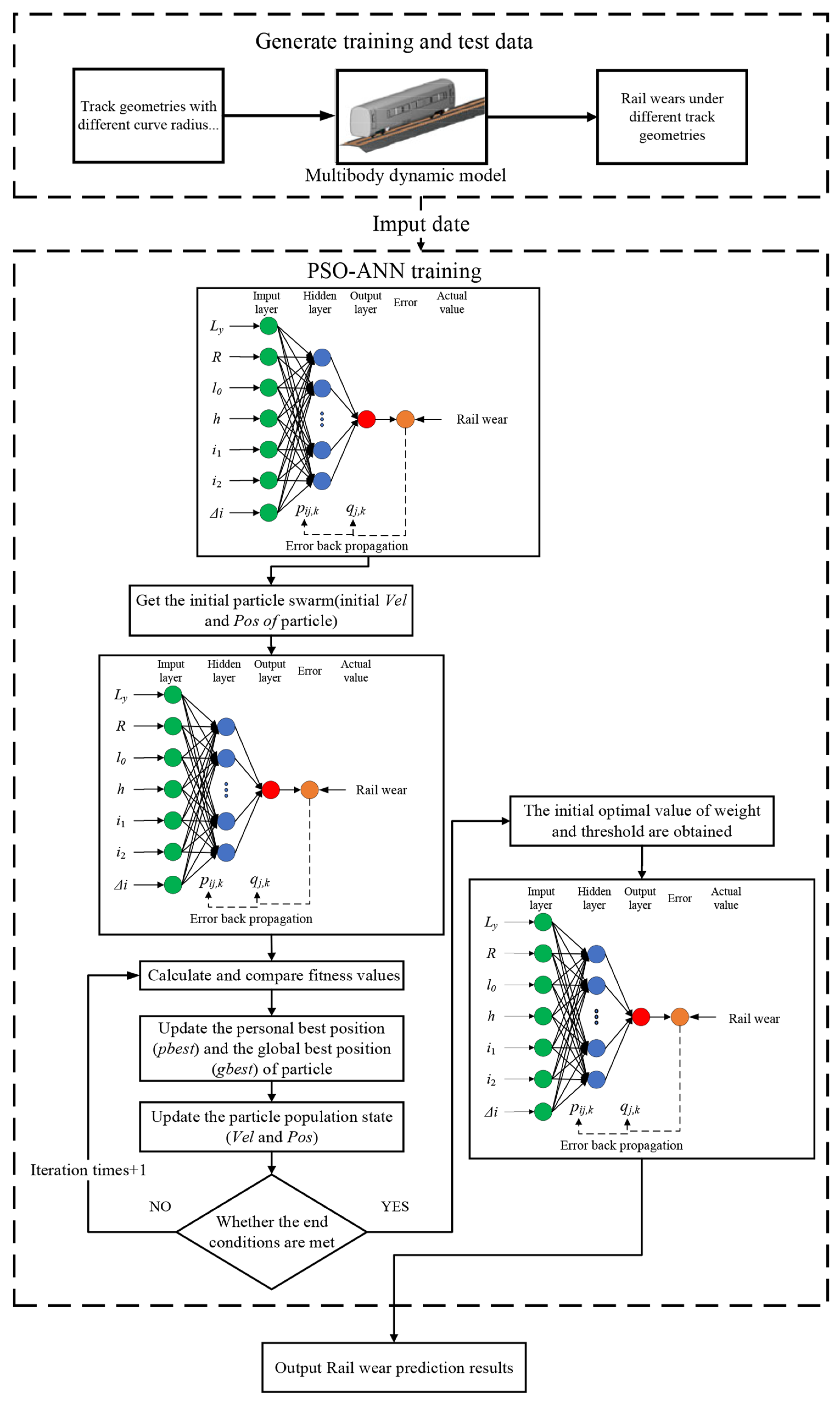
3.2. An Improved ANN Based on PSO (PSO-ANN)

The performance of the ANN model is highly sensitive to the initial weights. For the conventional ANN model, the initial weights are randomly generated, which may cause network oscillation and non-convergence [31]. To address this problem, particle swarm optimization (PSO) is employed to optimize the initial weights of the ANN model. PSO is an optimization technique that iteratively enhances a candidate solution based on a quality metric. It works by maintaining a population of candidate solutions, referred to as particles, and adjusting their positions in the search space to locate the optimal solution. Each particle has a fitness value and a velocity value. The fitness value is determined by the problem’s objective function, while the velocity dictates the direction and speed of movement.

In each iteration, the particle’s velocity is adjusted based on its current velocity and two best positions: the personal best (pbest) and the global best (gbest). The pbest is the best position a particle has achieved individually, and the gbest is the best position discovered by the entire swarm. The particle’s position is then updated according to its current position and the new velocity [32], as shown in Equations (14) and (15):

$$Ve{l}_i(t+1)=w\cdot Ve{l}_i(t)+C_1\cdot r_1(t)\cdot \left[gbest\left(t\right)-Po{s}_i\left(t\right)\right]+C_2\cdot r_2(t)\cdot \left[pbest\left(t\right)-Po{s}_i\left(t\right)\right]$$

(14)

$$Po{s}_i(t+1)=Po{s}_i\left(t)+Ve{l}_i\right(t+1)$$

(15)

where Vel and Pos denote the velocity and position of the particle, the lower foot label i denotes the ith particle in the swarm, and t denotes the tth iteration; C₁ and C₂ are acceleration coefficients, whose most frequent values are C₁ = C₂ = 2 [33]; r₁ and r₂ are random numbers that are uniformly distributed in the range [0, 1], and w is the inertia weight proposed by Shi and Eberhart [34].

The pseudocode of the optimization process is shown in Algorithm 1 as follows:

Algorithm 1: The Pseudocode of the Optimization Process [35]

Input: Track geometry parameters include curve radius (Ly), circular curve length (R), transition curve length (l0), superelevation (h), gradient (i1, i2), and gradient algebraic difference (Δi) Output: The final optimized neural network parameters Define the PSO parameters (number of particles, maximum iterations, and other related parameters) Initialize the particle swarm Initialize ANN model structure (input layer, hidden layers, output layer) For each particle Initialize particle End Do For each particle Calculate fitness value If the fitness value is better than the historical best (pbest) Update pbest to the current value. End Choose the particle with the best fitness value of all the particles as the gbest For each particle Calculate particle velocity according Equation (13) Update particle position according Equation (14) If max iterations or min error criteria are achieved End Return initial optimal value of weight and threshold

For the PSO-ANN model proposed in this study, the training starts with PSO, which performs a global search on weight ranges and finds the best initial weights for the neural network. Then, the back propagation (BP) algorithm starts the training process with the best initial weights provided by PSO.

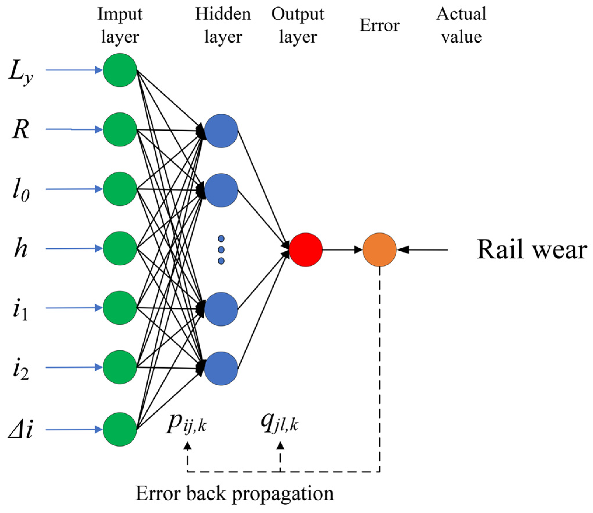
3.3. Rail Wear Prediction Based on PSO-ANN

In this study, the primary goal is to predict rail wear under different railway track geometries in order to evaluate a wide range of track geometries and thereby enhance the quality of railway alignment design. The track geometry can be characterized by a set of horizontal and vertical alignment parameters, including curve radius (L_y), circular curve length (R), transition curve length (l₀), superelevation (h), gradient (i₁, i₂), and gradient algebraic difference (Δi). Therefore, in this study, these alignment parameters are set as input data of the PSO-ANN models, and the rail wear is set as the output data, as shown in Figure 8.

To generate the training data of the PSO-ANN models, different values of horizontal and vertical alignment parameters are set according to the requirements of the Code for Design of Railway Line, and the corresponding rail wear is calculated through dynamic simulations in Section 2. It should be noted that other parameters affecting rail wear, such as speed, axle load, wheel profile, track substructure, and wheel-rail material [36,37,38], are kept constant and remain unchanged. The PSO-ANN models are trained using the generated data. Upon completion of the training, the model can predict rail wear for a railway track according to its horizontal and vertical alignment parameters (i.e., L_y, R, l₀, h, i₁, i₂, Δi). The whole process of rail wear prediction is shown in Figure 9.

4. Numerical Experiment Results and Discussions

In this section, 220 railway track geometries were randomly generated in accordance with the requirements of the Code for Design of Railway Line [39]. The corresponding rail wear for each track geometry is then calculated through dynamic simulations as detailed in Section 2, resulting in a total of 220 samples. Among these 220 samples, 150 samples are used to train the ANN models and the PSO-ANN models proposed in Section 3, and 70 samples are used to test the performance of these models. The computer equipped with a 13th Gen Intel(R) Core (TM) i9-13900K processor and 128 GB of random-access memory is used to perform the experiments, and the results are discussed as follows.

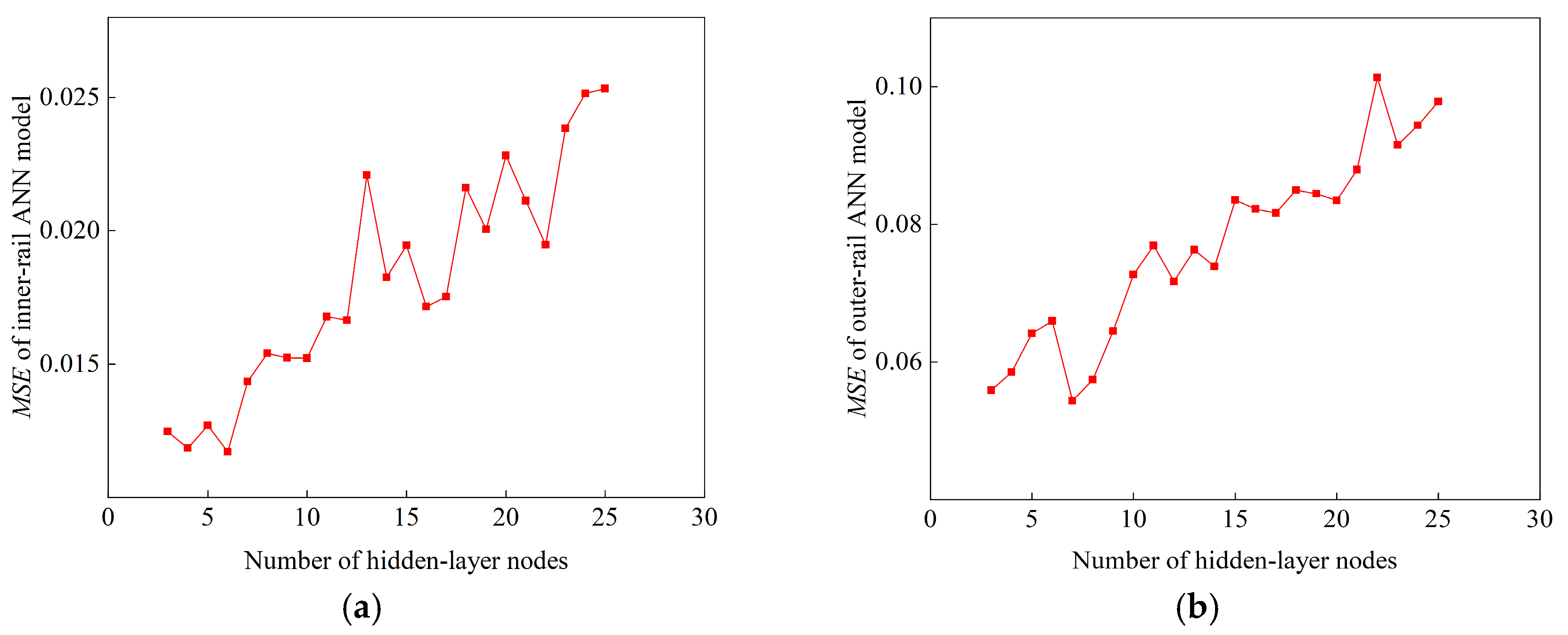
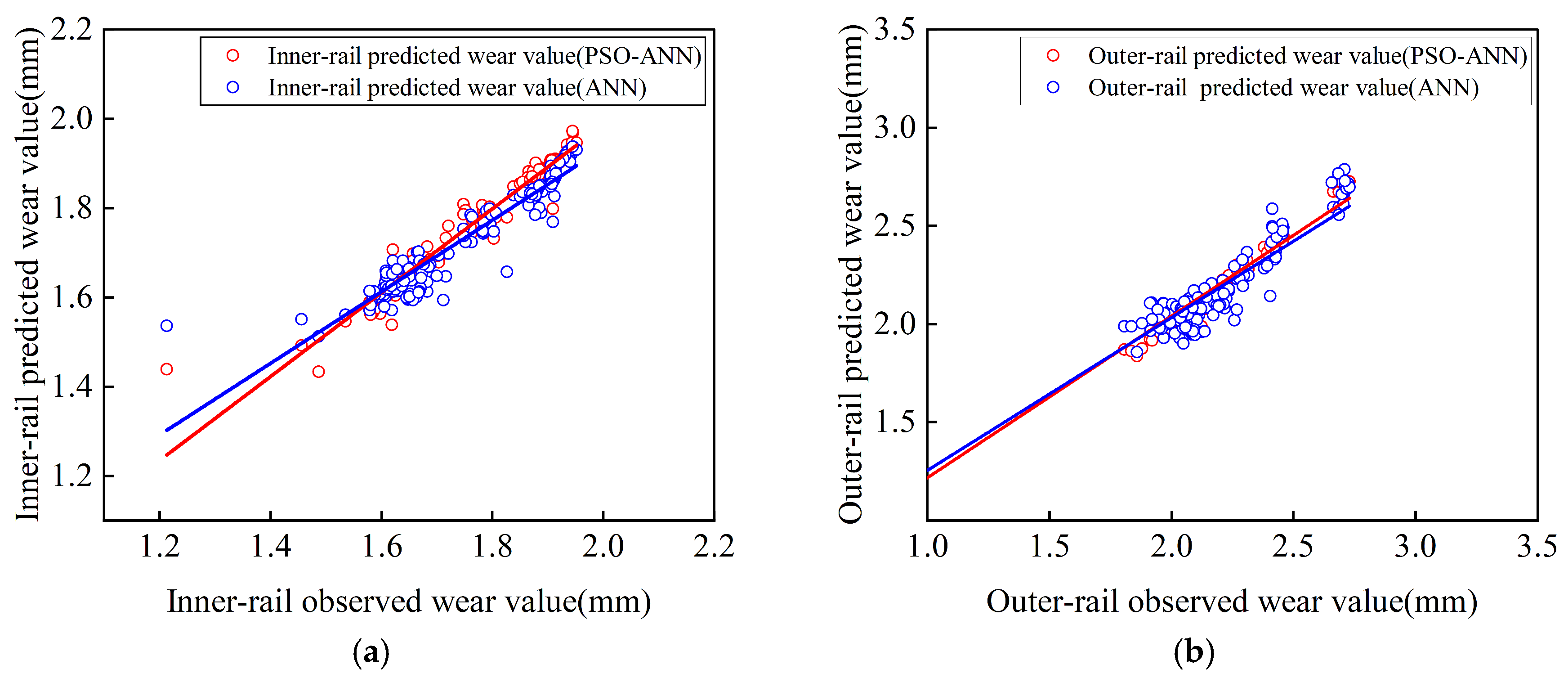
4.1. Prediction Accuracy of the ANN

The wear characteristics of the inner and outer rails differ significantly. For the inner rail, wear is predominantly concentrated on the top surface, whereas the outer rail experiences wear on both the top and side surfaces. Therefore, two separate ANN models, termed as inner and outer rail ANN models, have been developed to predict wear of inner and outer rails, respectively. Both models utilize the same input data, which includes curve radius, circular curve length, transition curve length, superelevation, gradients, and the algebraic difference of gradients. The optimal number of hidden-layer nodes for each model was determined separately through a trial-and-error method based on the training data, as shown in Figure 10. The inner rail ANN model was found to perform best with 6 hidden-layer nodes; the value of mean square error (MSE), which is expressed by Equation (16) [40], becomes minimum, while the outer rail ANN model required 7 nodes for optimal performance. Ultimately, the output of these ANN models are rail wear.

$$MSE={\displaystyle \frac{1}{D}}{\displaystyle \sum _{d=1}^D{(y_d^{*}-y_d)}^2}$$

(16)

where $y_d^{*}$ is the observed value of rail wear (through dynamic simulations); y_d is the predicted value of rail wear by the ANN model.

The predicted and observed values of rail wear are plotted as the horizontal and vertical coordinates, respectively, and a linear fit is applied to the data, as shown in Figure 11. The slope of the fitted line serves as an indicator of the ANN models’ performance, with a slope closer to 1 indicating better model accuracy. For the inner and outer rail ANN models, the slopes of the fitted lines are 0.802 and 0.778, respectively.

For the test data, the discrepancies between the predicted and observed rail wear values are shown in Figure 12. The mean absolute percentage error (MAPE) for the inner and outer rail ANN models are 4.26% and 4.22%, respectively, corresponding to accuracies of 95.74% and 95.78%.

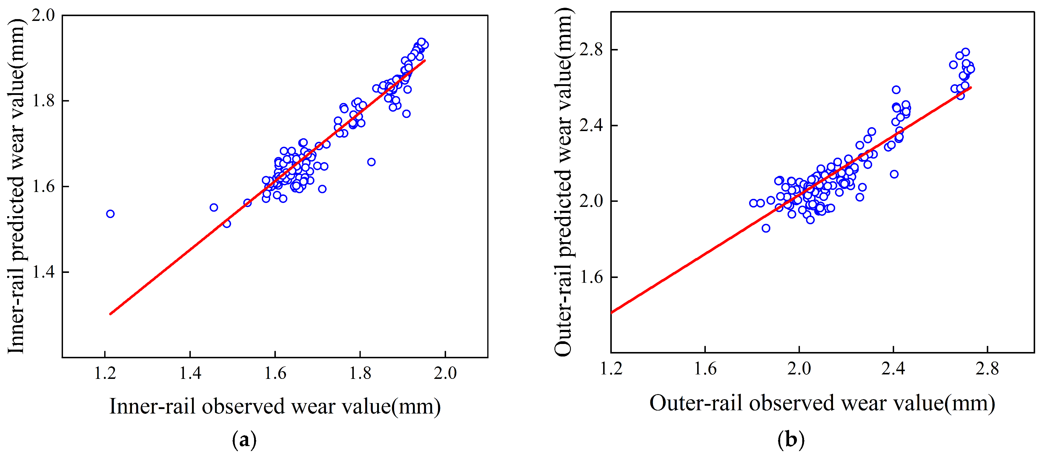
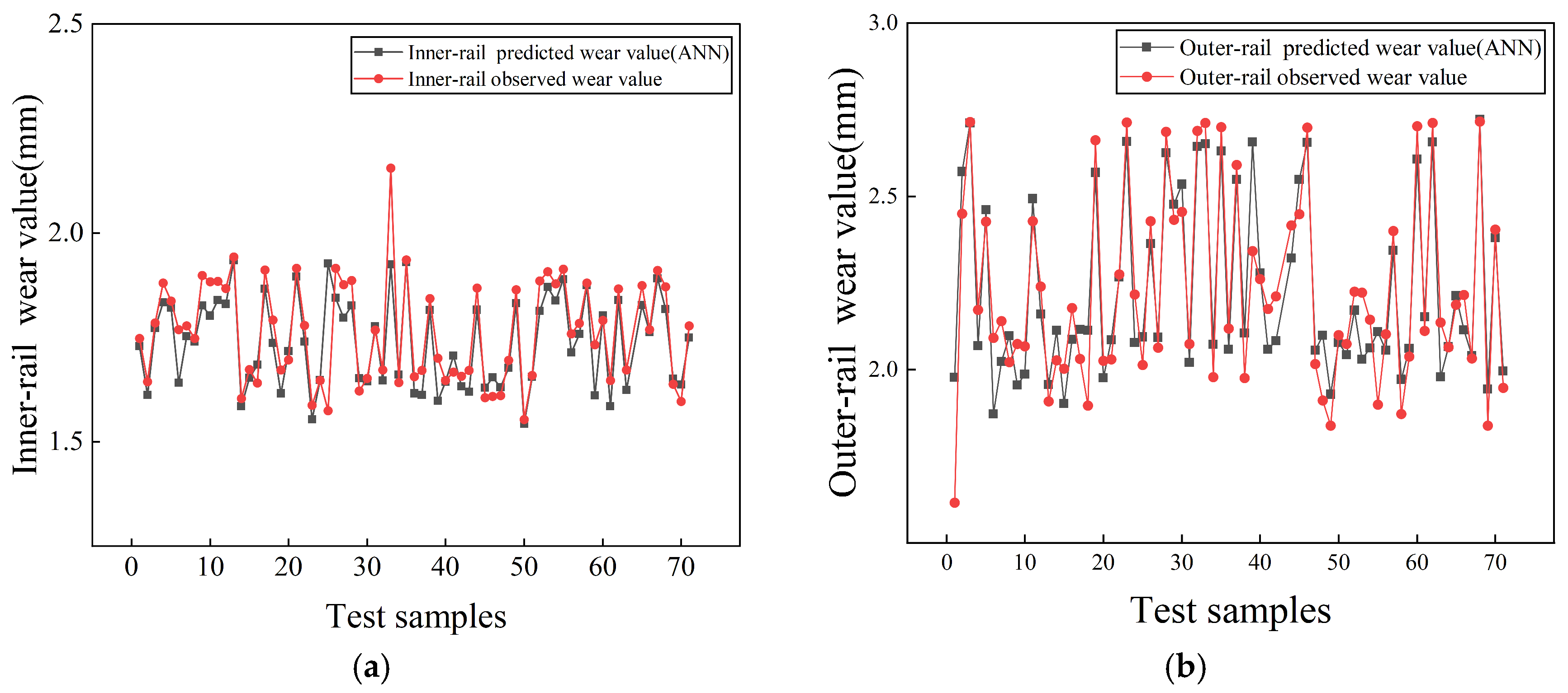
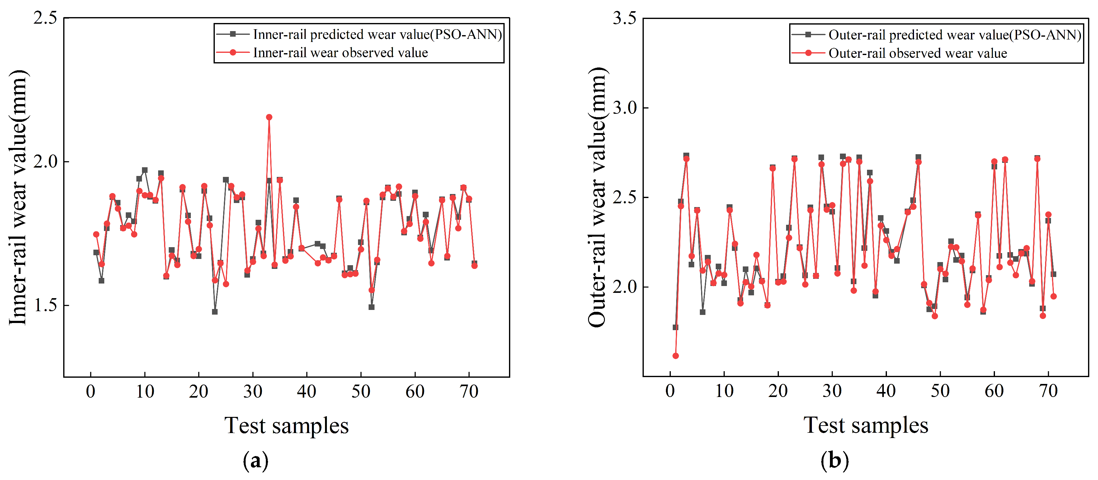
4.2. Prediction of the PSO-ANN

The predicted rail wear values from both the PSO-ANN models and ANN models, along with their corresponding observed values, are shown in Figure 13. It can be seen that for both the inner and outer rails, the correlation between predicted and observed rail wear values is stronger for the PSO-ANN models compared to the ANN models. The slopes of the fitting lines for the inner and outer rail PSO-ANN models are 0.940 and 0.832, respectively, both higher than those of the ANN models (0.802 and 0.778, respectively). These results demonstrate that the PSO-ANN models outperform the ANN models in predicting rail wear.

Figure 14 shows the discrepancies between the predicted and observed rail wear values from the PSO-ANN models for the test data. The mean absolute percentage errors (MAPE) for the inner and outer rail PSO-ANN models are 3.30% and 1.87%, respectively, representing reductions of 22.54% and 55.69% compared to the ANN models. Correspondingly, the prediction accuracies of the PSO-ANN models are 96.7% for the inner rail and 98.13% for the outer rail.

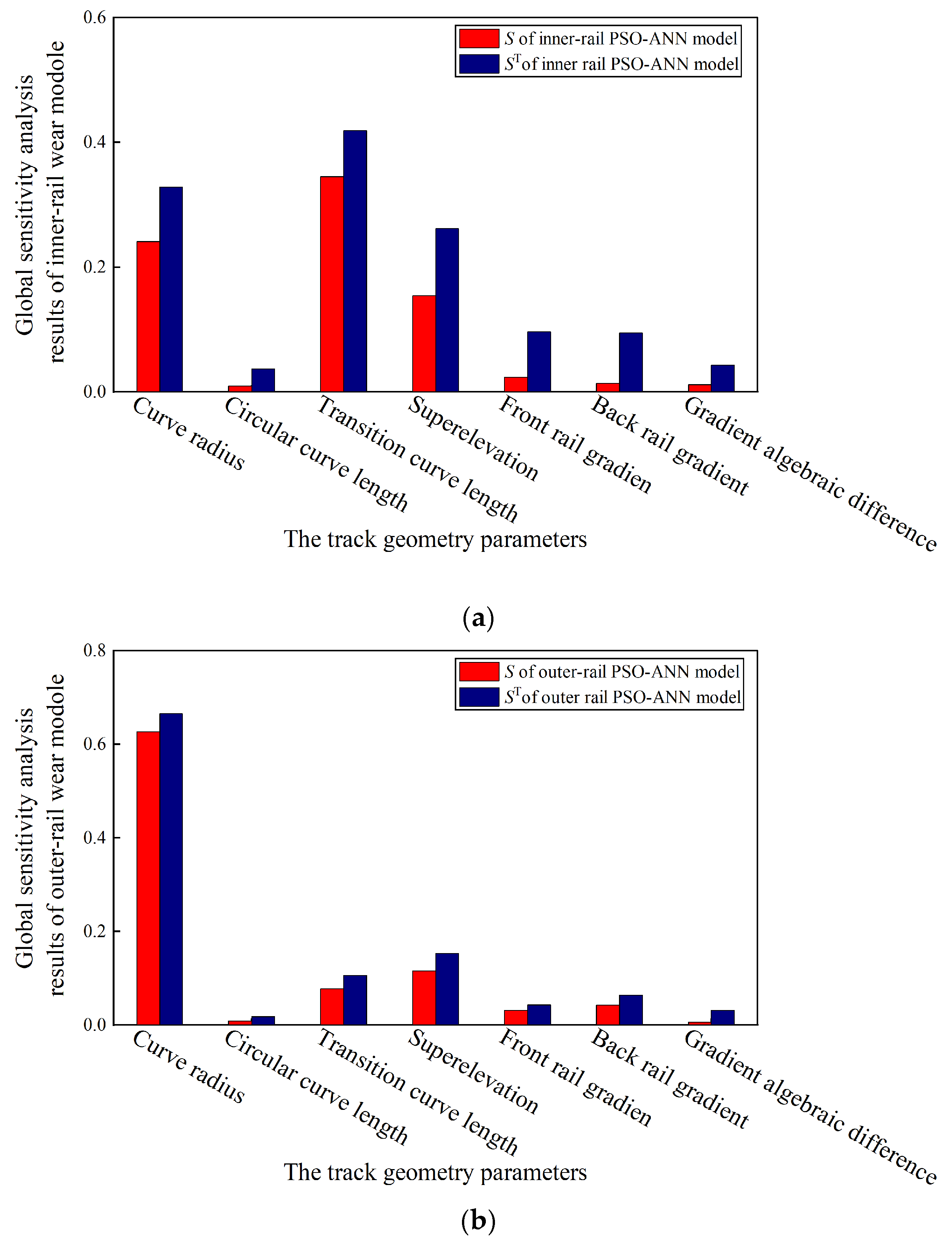
4.3. Sensitivity Analyses

Sensitivity analyses of the track geometry parameters (i.e., curve radius, circular curve length, transition curve length, superelevation, gradient, and gradient algebraic difference) on inner and outer rail wear are performed using Sobol’s analysis method [41,42,43]. All parameters can vary simultaneously during analysis, allowing the assessment of individual parameter effects and their interaction impacts on rail wear. The results are presented in Figure 15. The first-order sensitivity S_i (i = 1~7) indicates the individual influence of each parameter on rail wear, while the total sensitivity $S_i^T$ (i = 1~7), together with S_i, reflects the interaction of each parameter with all other parameters on impacting the rail wear. The greater the difference between S_i and $S_i^T$, the stronger the interaction effect of the parameter with others on impacting the rail wear.

From Figure 15, it can be seen that

• Different geometry parameters have varying effects on rail wear, and for the same geometry parameter, the impacts on the inner and outer rail wear also differ.
• For the inner-rail, transition curve length has the greatest influence, followed by curve radius and superelevation, while the effects of circular curve length and gradient algebraic difference are minimal.
• For the outer rail, the curve radius has the most significant individual effect and interaction with other parameters, as lateral wear, largely influenced by curve radius, is a major factor in outer-rail wear. The effects of transition curve length, superelevation, and gradient are comparatively smaller, with curve length and algebraic gradient difference having the least impact.

A comparative analysis of rail wear is conducted under varying curve radius (R), using the control variable method. The simulation results are presented in Figure 16.

From Figure 16, it is evident that the radius of the circular curve significantly affects the wear of the outer rail, as the rail wear profile varies greatly across different radii. In contrast, the wear of the inner rail is not significantly affected by the circular curve radius, as the rail wear profiles remain nearly unchanged across varying radii. However, according to the Sobol sensitivity analysis, the circular curve radius is identified as a key factor affecting inner rail wear. This is primarily due to its strong interaction effects with other parameters. These interaction effects cannot be captured by the control variable method, which isolates individual parameters and therefore fails to reflect the true influence of the circular curve radius on inner rail wear.

5. Conclusions

This paper developed an Artificial Neural Network model enhanced by Particle Swarm Optimization (PSO-ANN) to predict rail wear under different railway track geometries. This model serves as an efficient alternative to computationally intensive dynamic simulations, allowing for the rapid evaluation of a wide range of track geometries and thereby improving the quality of railway alignment design. The main contributions of this paper are summarized as follows:

• A PSO-ANN model was developed to predict the rail wear under different railway track geometries. The input data were the geometric parameters of the railway, which are curve radius, circular curve length, transition curve length, superelevation, gradient, and gradient algebraic difference, while the output data were the rail wear. The PSO-ANN model was able to predict the wear of the inner rail and outer rail with accuracies of 96.7% and 98.13%, demonstrating the good performance of the model. Compared with the conventional ANN model, the prediction errors can be reduced by 22.54% and 55.69%, respectively.
• Sobol analysis is used to assess the sensitivities of track geometry parameters to rail wear. The results indicate that for the inner rail, the primary factors influencing rail wear are the curve radius, transition curve length, and superelevation, while for the outer rail, the curve radius is the most significant factor.

The developed PSO-ANN model enables alignment design engineers to rapidly assess the quality of the alignment and make informed design decisions. Additionally, Sobol sensitivity analysis results from the model can assist alignment design engineers in identifying critical sections and optimizing the geometry parameters in these sections to improve the quality of the alignment.

Future research will analyze the impact of varying wheel-rail friction coefficients and worn wheels on rail wear. Meanwhile, we will measure rail wear in real-world railways and incorporate this data into the training and testing datasets. Additionally, the trained PSO-ANN model will be integrated into railway alignment optimization models [44,45]. By considering rail wear during the design phase and optimizing the railway alignment, the rail wear can be reduced from the source.

References

1. Liu, J.; Wang, W.; Liu, Q. Matching Characteristics between Four Kinds of Wheel Steels and U71Mn Hot-Rolled Rail. J. Southwest Jiaotong Univ. 2015, 50, 1130–1135. (In Chinese) [Google Scholar]
2. Wang, J.; Chen, X.; Li, X.; Wu, Y. Influence of heavy haul railway curve parameters on rail wear. Eng. Fail. Anal. 2015, 57, 511–520. [Google Scholar] [CrossRef]
3. Ignesti, M.; Malvezzi, M.; Marini, L.; Meli, E.; Rindi, A. Development of a wear model for the prediction of wheel and rail profile evolution in railway systems. Wear 2012, 284, 1–17. [Google Scholar] [CrossRef]
4. Wang, P.; Wang, S.; Si, D. Numerical prediction of rail wear development in high-speed railway turnouts. Proceedings of the Institution of Mechanical Engineers. J. Rail Rapid Transit 2020, 234, 1299–1318. [Google Scholar] [CrossRef]
5. Li, X.; Yang, T.; Zhang, J.; Cao, Y.; Wen, Z.; Jin, X. Rail wear on the curve of a heavy haul line-Numerical simulations and comparison with field measurements. Wear 2016, 366–367, 131–138. [Google Scholar] [CrossRef]
6. Sun, Y.; Guo, Y.; Zhai, W. Prediction of rail non-uniform wear-influence of track random irregularity. Wear 2019, 420, 235–244. [Google Scholar] [CrossRef]
7. Wen, B.; Wang, S.; Tao, G.; Li, J.; Ren, D.; Wen, Z. Prediction of rail profile evolution on metro curved tracks: Wear model and validation. Int. J. Rall Transp. 2022, 11, 811–832. [Google Scholar] [CrossRef]
8. Wang, H.; Zhao, Y.; Qi, Y.; Cao, Y. Effect of line parameters on wheel wear of heavy–haul freight vehicle. Ind. Lubr. Tribol. 2024, 76, 419–430. [Google Scholar] [CrossRef]
9. Meghoe, A.; Loendersloot, R.; Tinga, T. Rail wear and remaining life prediction using meta-models. Int. J. Rail Transp. 2020, 8, 1–26. [Google Scholar] [CrossRef]
10. Yin, X.; Kou, L.; Wei, X. Side wear prediction of a subway outer rail on small radius curves based on system dynamics of discrete supported track. Discret. Dyn. Nat. Soc. 2022, 2022, 7037655. [Google Scholar] [CrossRef]
11. Zhou, Y. Analysis of rail wear Influencing factors and study on prediction of wear. Transp. Energy Conserv. Environ. Prot. 2018, 14, 8–10. (In Chinese) [Google Scholar] [CrossRef]
12. Wang, P.; Wang, C.; Wang, W.; Liu, Q. Application of BP ANN optimized by hybrid algorithm based on POS in wear volume prediction of rail steel. J. Mech. Des. 2013, 30, 15–20. (In Chinese) [Google Scholar] [CrossRef]
13. Gao, T.; Wang, Q.; Yang, K.; Yang, C.; Wang, P.; He, Q. Estimation of rail renewal period in small radius Curves: A data and mechanics integrated approach. Measurement 2021, 185, 9. [Google Scholar] [CrossRef]
14. Jin, X.; Wen, Z.; Xiao, X.; Zhou, Z. A numerical method for prediction of curved rail wear. Multibody Syst. Dyn. 2007, 18, 531–557. [Google Scholar] [CrossRef]
15. Liu, Q.; Tao, G.; Liang, H.; Lu, C.; Wen, Z.; Long, H. Influence of metro wheel polygonal wear on dynamic properties of wheel-rail system. J. Cent. South Univ. (Sci. Technol.) 2022, 53, 3222–3231. (In Chinese) [Google Scholar] [CrossRef]
16. Wang, Z.; Lei, Z. Development characteristics of rail wear under different curve radius of metro. Railw. Eng. 2020, 60, 134–137. (In Chinese) [Google Scholar]
17. Wang, L.; Zhang, X.; Liu, H.; Han, Y.; Zhu, Z.; Cai, C. Global reliability analysis of running safety of a train traversing a bridge under crosswinds. J. Wind. Eng. Ind. Aerodyn. 2022, 224, 104979. [Google Scholar] [CrossRef]
18. Li, Z.; Kalker, J. Simulation of severe wheel-rail wear. WIT Press. 1998, 37, 393–402. [Google Scholar]
19. De Arizon, J.; Verlinden, O.; Dehombreux, P. Prediction of wheel wear in urban railway transport: Comparison of existing models. Veh. Syst. Dyn. 2007, 45, 849–866. [Google Scholar] [CrossRef]
20. Wang, S.; Qian, Y.; Feng, Q.; Guo, F.; Rizos, D.; Luo, X. Investigating high rail side wear in urban transit track through numerical simulation and field monitoring. Wear 2021, 470, 203643. [Google Scholar] [CrossRef]
21. Piotrowski, J.; Kik, W. A simplified model of wheel/rail contact mechanics for non-Hertzian problems and its application in rail vehicle dynamic simulations. Veh. Syst. Dyn. 2008, 46, 27–48. [Google Scholar] [CrossRef]
22. Sun, Y.; Ling, L. An optimal tangential contact model for wheel-rail non-Hertzian contact analysis and its application in railway vehicle dynamics simulation. Veh. Syst. Dyn. 2021, 60, 3240–3268. [Google Scholar] [CrossRef]
23. TG/GW102-2023; China State Railway Group Co., Ltd. Rules for the Repair of General-Speed Railway Lines. China Railway Publishing House: Beijing, China, 2023.
24. TG/GW121-2014; China State Railway Group Co., Ltd. Safety Regulations for High-Speed Railway Maintenance (Trial). China Railway Publishing House: Beijing, China, 2014.
25. Kramer, M. Nonlinear principal component analysis using autoassociative neural networks. Aiche J. 1991, 37, 233–243. [Google Scholar] [CrossRef]
26. Hornik, K.; Stinchcombe, M.; White, H. Multilayer feedforward networks are universal approximators. Neural Netw. 1989, 2, 359–366. [Google Scholar] [CrossRef]
27. Liu, X.; Wang, Z.; Li, J. Global Sensitivity Analysis Method for Parameters of Storm Water Management Model Based on BP Neural Network. China Water Wastewater 2021, 37, 8. (In Chinese) [Google Scholar] [CrossRef]
28. Rubio, J.D. Stability Analysis of the Modified Levenberg-Marquardt Algorithm for the Artificial Neural Network Training. IEEE Trans. Neural Netw. Learn. Syst. 2021, 32, 3510–3524. [Google Scholar] [CrossRef]
29. Wang, M.; Jia, S.; Chen, E.; Yang, S.; Liu, P.; Qi, Z. Research and application of neural network for tread wear prediction and optimization. Mech. Syst. Signal Process. 2022, 162, 108070. [Google Scholar] [CrossRef]
30. Ren, C.; An, N.; Wang, J.; Li, L.; Hu, B.; Shang, D. Optimal parameters selection for BP neural network based on particle swarm optimization: A case study of wind speed forecasting. Knowl.-Based Syst. 2014, 56, 226–239. [Google Scholar] [CrossRef]
31. Huang, K.; Zhang, W.; Zhang, Y. Research on shield parameter prediction based on the PSO-RF hybrid algorithm. J. Transp. Sci. Eng. 2024, 40, 117–127. [Google Scholar] [CrossRef]
32. Ding, F.; Jia, X.; Hong, T.; Xu, Y. Flow stress prediction model of 6061 aluminum alloy sheet based on GA-BP and PSO-BP neural networks. Rare Met. Mater. Eng. 2020, 49, 1840–1853. [Google Scholar]
33. Pu, H.; Song, T.; Schonfeld, P.; Li, W.; Zhang, H.; Hu, J.; Peng, X.; Wang, J. Mountain railway alignment optimization using stepwise & hybrid particle swarm optimization incorporating genetic operators. Appl. Soft Comput. 2019, 78, 41–57. [Google Scholar] [CrossRef]
34. Shi, Y.; Eberhart, R. A modified particle swarm optimizer. In Proceedings of the 1998 IEEE World Conference on Evolutionary Computation, Anchorage, AK, USA, 4–9 May 1998. [Google Scholar]
35. Kadadevaramath, R.S.; Mohanasundaram, K.M.; Rameshkumar, K.; Chandrashekhar, B. Production and distribution scheduling of Supply Chain structure using intelligent Particle Swarm Optimisation algorithm. Int. J. Intell. Syst. Technol. Appl. 2009, 6, 249–268. [Google Scholar] [CrossRef]
36. Ma, X.; Yin, W.; Wang, Y.; Liu, L.; Wang, X.; Qian, Y. Fatigue failure analysis of U75V rail material under Ⅰ + Ⅱ mixed-mode loading: Characterization using peridynamics and experimental verification. Int. J. Fatigue 2024, 185, 108371. [Google Scholar] [CrossRef]
37. Ma, X.; Wang, Y.; Wang, X.; Yin, W.; Liu, L.; Xu, J. Investigation on fatigue crack propagation behaviour of U71Mn and U75V rails using peridynamics. Eng. Fract. Mech. 2023, 281, 109097. [Google Scholar] [CrossRef]
38. Zhu, X.; Xu, J.; Li, Y.; Hou, M.; Qian, Y.; Wang, P.; Chen, J.; Yan, Z. Load spectrum extrapolation method for fatigue damage of the turnout based on kernel density estimation. Eng. Fail. Anal. 2024, 160, 108169. [Google Scholar] [CrossRef]
39. GB 50157-2013; Ministry of Housing and Urban-Rural Development of the People’s Republic of China. Code for Design of Metro. China Architecture & Building Press: Beijing, China, 2014.
40. Jiang, H.; Gao, L. Optimizing the Rail Profile for High-Speed Railways Based on Artificial Neural Network and Genetic Algorithm Coupled Method. Sustainability 2020, 12, 658. [Google Scholar] [CrossRef]
41. Sobol′, I. Global sensitivity indices for nonlinear mathematical models and their monte carlo estimates. Math. Comput. Simul. 2001, 55, 271–280. [Google Scholar] [CrossRef]
42. Saltelli, A.; Annoni, P.; Azzini, I.; Campolongo, F.; Ratto, M.; Tarantola, S. Variance based sensitivity analysis of model output. Design and estimator for the total sensitivity index. Comput. Phys. Commun. 2010, 181, 259–270. [Google Scholar] [CrossRef]
43. Pineda-Jaramillo, J.; Martínez-Fernández, P.; Villalba-Sanchis, I.; Salvador-Zuriaga, P.; Insa-Franco, R. Predicting the traction power of metropolitan railway lines using different machine learning models. Int. J. Rail Transp. 2020, 9, 461–478. [Google Scholar] [CrossRef]
44. Song, T.; Pu, H.; Yang, T.Y.; Schonfeld, P.; Li, W.; Hu, J. Optimizing net present values of risk avoidance for mountain railway alignments with seismic performance evaluation. Comput.-Aided Civ. Infrastruct. Eng. 2024, 39, 944–962. [Google Scholar] [CrossRef]
45. Song, T.; Pu, H.; Yang, T.Y.; Schonfeld, P.; Wan, X.; Li, W.; Zhu, Z.; Zhang, H.; Hu, J. Modeling earthquake-induced landslide risk for mountain railway alignment optimization. ASCE-ASME J. Risk Uncertain. Eng. Syst. Part A Civ. Eng. 2024, 10, 04024005. [Google Scholar] [CrossRef]
Figure 1. Rail wear estimation process by means of numerical experiments [9].
Infrastructures 10 00154 g001
Figure 2. Dynamic model of the vehicle structure. (a) Side view. (b) Front view. (c) Top view [17].
Infrastructures 10 00154 g002
Figure 3. Diagram of discretization of the wheel–rail contact spot.
Infrastructures 10 00154 g003
Figure 4. Rail wear simulation flowchart.
Infrastructures 10 00154 g004
Figure 5. Rail wear measurement standard.
Infrastructures 10 00154 g005
Figure 6. Simulation results of rail wear.
Infrastructures 10 00154 g006
Figure 7. Structure of an artificial neural network.
Infrastructures 10 00154 g007
Figure 8. Structure of Artificial neural network in the PSO-ANN model.
Infrastructures 10 00154 g008
Figure 9. Flowchart of rail wear prediction.
Infrastructures 10 00154 g009
Figure 10. The relationship between the number of hidden-layer nodes and MSE. (a) Inner-rail wear ANN model. (b) Outer-rail wear ANN model.
Infrastructures 10 00154 g010
Figure 11. The predicted rail wear values of the ANN models and the corresponding observed values. (a) Inner-rail wear ANN model. (b) Outer-rail wear ANN model.
Infrastructures 10 00154 g011
Figure 12. Comparison between predicted and observed rail wear values for the test data. (a) Inner-rail wear ANN model. (b) Outer-rail wear ANN model.
Infrastructures 10 00154 g012
Figure 13. The predicted rail wear values of the PSO-ANN models, ANN models, and the corresponding observed values. (a) Inner-rail wear PSO-ANN model. (b) Outer-rail wear PSO-ANN model.
Infrastructures 10 00154 g013
Figure 14. Comparison between predicted and observed rail wear values for the test data. (a) Inner-rail wear PSO-ANN model. (b) Outer-rail wear PSO-ANN model.
Infrastructures 10 00154 g014
Figure 15. Global sensitivity analysis results. (a) Inner-rail wear PSO-ANN model. (b) Outer-rail wear PSO-ANN model.
Infrastructures 10 00154 g015
Figure 16. Relationship between inner and outer rail wear and radius of circular curve. (a) Inner-rail. (b) Outer rail.
Infrastructures 10 00154 g016