Abstract
Exposure modeling plays a crucial role in disaster risk assessments by providing geospatial information about assets at risk and their characteristics. Detailed exposure data enhances the spatial representation of a rapidly changing environment, enabling decision-makers to develop effective policies for reducing disaster risk. This work proposes and demonstrates a methodology linking volunteered geographic information from OpenStreetMap (OSM), street-level imagery from Google Street View (GSV), and deep learning object detection models into the automated creation of exposure datasets for power grid transmission towers, assets particularly vulnerable to strong wind, and other perils. Specifically, the methodology is implemented through a start-to-end pipeline that starts from the locations of transmission towers derived from OSM data to obtain GSV images capturing the towers in a given region, based on which their relevant features for risk assessment purposes are determined using two families of object detection models, i.e., single-stage and two-stage detectors. Both models adopted herein, You Only Look Once version 5 (YOLOv5) and Detectron2, achieved high values of mean average precision (mAP) for the identification task (83.67% and 88.64%, respectively), while Detectron2 was found to outperform YOLOv5 for the classification task with a mAP of 64.89% against a 50.62% of the single-stage detector. When applied to a pilot study area in northern Portugal comprising approximately 5.800 towers, the two-stage detector also exhibited higher confidence in its detection on a larger part of the study area, highlighting the potential of the approach for large-scale exposure modeling of transmission towers.
1. Introduction
The built environment is constantly under the threat of natural hazards, and climate change will only exacerbate such perils [1]. The assessment of natural hazard risk requires exposure models representing the characteristics of the assets at risk, which are crucial to subsequently estimate damage and impacts of a given hazard to such assets [2]. Therefore, the exposure modeling of the built environment provides a basis for decision makers to establish policies and strategies to reduce disaster risk [3], offering geospatial information with a fine level of spatial detail regarding an often hard to track and rapidly changing built environment [4]. Therefore, studies addressing the exposure modeling of the built environment are expanding, supported by the emergence of new modeling possibilities associated with technological progress. In fact, multiple works introduce data collected from volunteered geographic information (VGI), user-generated content, and remote sensing data in natural hazards analysis. Still, many issues with the quality of the data, their reliability, and the spatial coverage of these type of data remains [5,6]. These methods generate large amounts of data that typically require a time-consuming extraction of the necessary information. This labor-intensive task is well suited for the capability of machine learning (ML) models, particularly deep learning models, to handle massive amounts of data [7]. The use of deep learning models has found several applications in the risk modeling of buildings, where artificial intelligence is used for a variety of reasons. For example, ref. [8] use an ML classifier ensemble method to combine OpenStreetMap and remote sensing data and extract exposure information regarding the number of buildings and the distribution of the population in the territory of Valparaíso, Chile. Several studies involve the use of deep learning models to extract information about the characteristics of buildings in urban areas (e.g., type of structures, numbers of floors, number of windows, type of roof) that are then used to perform seismic risk assessments [9,10]. Ref. [11] use a deep learning model to estimate the number of floors for each building in an urban setting based on street-level imagery. Other studies focused on improving damage assessment of the roof or the entire building by using a deep learning model in conjunction with aerophoto images that are taken during the event [12]. Similarly, deep learning models have also been applied in the field of electrical infrastructure with a special focus on detecting transmission towers in images [13,14]. However, the current state of the art is rather limited in number and scope, as most studies focus solely on tower inspection and management or rely on images retrieved via drones. Given the essential role that power lines play in delivering electricity to homes, businesses, and vital services, the risks posed by their damage during natural disasters remain understudied and poorly understood, exacerbating disaster impact [15,16]. The current work provides a comprehensive approach aimed at enhancing risk assessments. In this context, the present article proposes a methodology that connects VGI obtained from OpenStreetMap (OSM), street-level imagery from Google Street View (GSV), and deep learning object detection models to create an exposure dataset of electrical transmission towers, an asset type particularly vulnerable to strong winds as well as other perils, such as ice loads and earthquakes [17,18,19]. The main objective of the study is to establish and demonstrate a complete pipeline that first obtains the locations of transmission towers from the power infrastructure in OSM data, and subsequently assigns relevant features of each tower based on the classification returned from an object detection model over street-level imagery of the tower, obtained from GSV. Additionally, two different object detection models belonging to different families (i.e., single-stage and two-stage detectors) are used to perform the task, and a comparison between the two is carried out. The article is structured as follows: Section 2 introduces the key components of the pipeline, highlighting their features and criticality, and describes the case study selected to pilot the methodology, the training procedures, and the data used. Section 3 presents the main findings of the work, emphasizing the differences among the two families of object detection models used. Lastly, Section 4 summarizes the most important take-home message of the study, limitations, and future developments that would improve the application of the presented methodology.
2. Materials and Methods
The proposed methodology connects VGI obtained from OpenStreetMap (OSM), street-level imagery from Google Street View (GSV), and deep learning object detection models into the creation of an exposure dataset of electrical transmission towers. First, OpenStreetMap data are used to obtain the location of electrical transmission towers at the large scale. Street-level imagery from Google Street View is then used to collect photographs where each tower is visible. Lastly, a deep learning detection model is used to classify each tower based on a set of classes that are previously defined based on a custom taxonomy of the most representative type of tower for the area under study. The workflow of the methodology is represented in Figure 1.
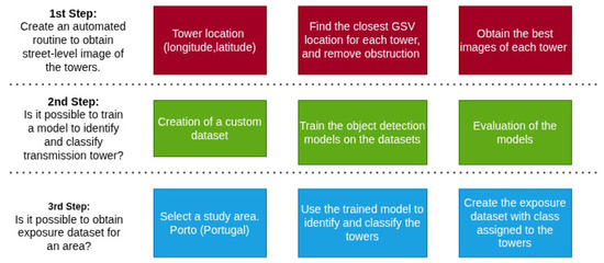
Figure 1.
Workflow of the proposed methodology.
2.1. Geospatial Data
2.1.1. OpenStreetMap (OSM)
OpenStreetMap (OSM) is an open geographic database of the world built and maintained by volunteers. The project started in 2004 and has gained great popularity over the years, motivated by technical and legal restrictions imposed by existing map services, which limited their applicability in innovative and creative applications [20]. As of today, the OSM project has more than 8 million registered users and the database is constantly being expanded and improved [21]. OSM uses three types of elements to coherently represent the physical world: nodes, ways, and relations. Nodes are the basic element of OSM’s data model. Each node represents a single point in space, to which a pair of coordinates (i.e., latitude and longitude) and a node ID are associated. Ways are an ordered list of nodes that are used to represent linear features like roads and rivers. Currently, there are over 8 billion nodes and 900 million ways in the OSM database. Lastly, a relation is a data structure describing logical or geographic relationships between elements, which can be used for multiple purposes. An example of a relation is the multi-polygon, which is used to represent complex areas. Elements can have one or more associated tags, which consists of a pair of a key and value that describe the function and/or peculiarity of the element [22]. The elements in the OSM database are divided into categories and sub-categories based on their tags. There are seven broad categories: (1) Leisure, Sport and Shopping, (2) Services, (3) Culture and Religion, (4) Transportation, (5) Infrastructure, (6) Places, and (7) Special. The Infrastructure category collects all kinds of physical infrastructure that are commonly found wherever human activities are carried out, including power distribution and production infrastructures. For this study, interest lies in the elements tagged as power with value equal to tower, which identifies large towers or pylons carrying electricity cables. The OSM database contains more than 14 million towers, but the level of detail of their distribution around the world is not homogeneous, as can be seen from the OSM-based OpenInfraMap (https://openinframap.org/). Different tools have been developed by third parties to facilitate the interaction between users and the OSM database [23]. In this study, the data were obtained using the Overpass API, a read-only API optimized for consuming data rather than editing, which is therefore reasonably fast for downloading large amounts of data. The Overpass API takes the user query with all the specified requirements of the search and returns the corresponding data in JSON format.
2.1.2. Street-Level Imagery with Google Street View (GSV)
In its simplest form, a street-level image is a representation of the landscape from the perspective of a pedestrian or a vehicle [24]. The most prominent promoter of street-level imagery is Google, which expanded the service provided by Google Maps and Google Earth by adding Google Street View [25]. Since its first release in 2007, GSV expanded its spatial coverage relentlessly, reaching up to 16 million km of road coverage [26]. Most of the images are taken by street view cars, but there is also a significant contribution from the community. For this purpose, Google provides a list of cameras that are suitable for taking pictures that can be uploaded to its platform. GSV provides an API that allows users to extract street-level imagery for a given location [27]. Additionally, the optional parameters allow for adjusting of different features of the image that one is downloading. The heading refers to the direction on a compass of the camera, with 0 and 360 both indicating the north going clockwise; the field of view grants the possibility to adjust the level of zoom of the image, with values within 0 and 120 (default is 90), where small values indicate a higher level of zoom; and the pitch allows the user to move the angle of the camera, which is usually flat horizontal, in the vertical direction. Positive values tilt the camera upward, while negative values tilt it downward. The right definition of these parameters is key in the extraction of the frame correctly picturing the tower. Another challenge is the possible existence of objects obstructing the view of a tower in an image, such as buildings, cars, or trees. In addition, the orography could hide part of an element, as well as infrastructures such as retaining walls. In this study, each of these challenges was addressed separately. The identification of the best parameters for retrieving the most accurate image was achieved by using the information relative to the location and elevation of each tower and the 4 closest points of GSV to each tower. This information allowed for computing of the heading and pitch, as exhibited in Figure 2a,b. After a trial-and-error phase, the field of view value was chosen based on a distance criterion. For distances less than 10 m between the tower and the GSV point, the default value was applied. In contrast, for distances over 600 m, a value of 15 was used, as it was the highest zoom level achievable without causing image blur. Finally, for distances in between, a linear interpolation of the field of view values was applied. The same information on location and elevation was used to discard the GSV point of view that may have yielded images containing buildings and/or orographic formations that might have obstructed the view of the GSV sensor. The footprints of the buildings were extracted from OSM and were used to control if any point of the perimeter of each building falls between the direct line connecting the tower to the GSV point of view; this way, it was possible to ensure that the least number of buildings would be captured in the GSV image (Figure 2c). In a similar manner, the orography was taken into consideration by drawing the elevation profile between each pair formed by the location of the tower and the GSV point of view for that location, ensuring that the straight lines connecting the pair with a peak in the middle were excluded. These steps ensured the highest number of images with a valid view of a tower, and the download was subsequently made through the Google Street View API. Additional detail on the equation used to derive GSV optimal parameters can be found in Appendix A.
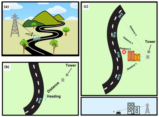
Figure 2.
Description of the different approach used to overcome the limitations of using street-level imagery. Definition of the best GSV parameters (a,b), elimination of obstructing buildings (c).
2.1.3. Study Area
The study area displayed in Figure 3, utilized for the initial application of the methodology, covers an area of 1360 km2 within the Porto district (Portugal). The area was found to be representative, given its diverse land use, containing both densely populated settlements and rural areas, and the different types of transmission towers that can be found. Within this area, the power infrastructure from the OpenStreetMap database contains 5789 transmission towers distributed across almost 680 km of electrical power lines. Retrieving the corresponding street-level imagery for each tower required the adoption of different strategies to overcome problems related to visibility, as described in the previous subsection. The building and road layers of OSM made it possible to remove GSV shots that were obstructed by buildings. Furthermore, the SRTM 30 m resolution digital elevation model (OpenTopography, San Diego, CA, USA, 2013) was used to remove camera shots that were hindered by the orography.
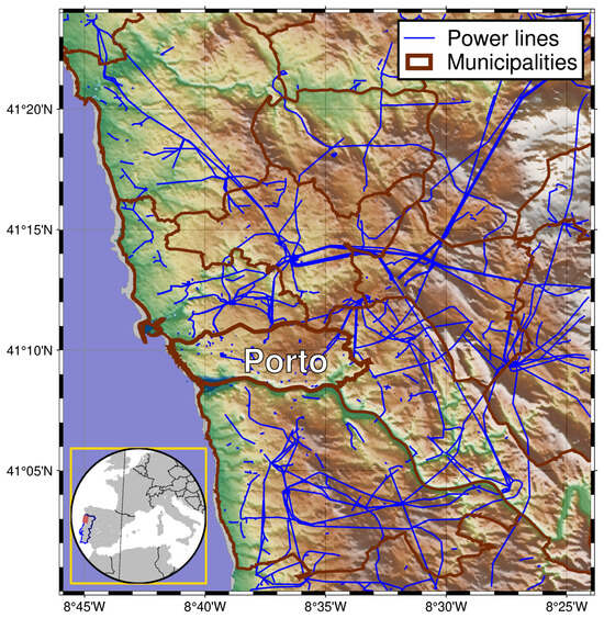
Figure 3.
Map of the power lines inside the study area.
2.2. Data Preparation
In the object detection field, it is common practice to test new advancements in architectures, loss functions, and tweaks in the algorithms using well-established datasets [28,29]. This way, it is possible for different researchers to measure the improvements brought by their novelties and compare the performance of the model over the same baseline. On the other hand, when the objective of the study is not to bring improvements to the model but using it in a real-life application (i.e., using the model to identify and classify towers), adopting already existing datasets could be detrimental towards achieving the best overall possible performance, as the dataset might not contain images for the class of interest or the accuracy of the image in describing the classes might not be good enough to reflect the outcome expected. Thus, in such cases, the training of the model requires the use of custom datasets [30]. In this work, two different tasks were carried out: identification and classification of electrical transmission towers. The first task was used to test the ability of a model to recognize whether a tower is present in an image, while the second task assigned a category to each tower based on a taxonomy derived from a compilation of the most used types of towers (Table 1) [31,32,33,34]. The taxonomy is based on the shape of the tower, which in turn, influences the structural behavior of the tower. In the taxonomy, three categories are defined: (a) self-supporting, (b) waist-type, and (c) monopole. For each category a different class is again assigned among the most common shapes. Classifying the towers is critical for assessing risk to this type of asset, as different tower types have different vulnerabilities and will sustain different levels of damage when impacted by natural perils.

Table 1.
Taxonomy of the tower’s classification.
The identification and classification tasks call for different levels of detail in the images used to train the models. For the first task, the image is required to only contain a transmission tower, while for the classification task, obtaining images with a class of the tower belonging to the taxonomy was indispensable. The images were automatically downloaded from three image search engines: Google, Bing, and Flickr. The taxonomy implemented leaves out possible transmission towers used in reality. While this might introduce some limitations to the generalizability of the methodology, using the most common classes was inevitable to be able to find images of the tower in the search engines, since the photos of specific underutilized towers are not to be found through searches. Therefore, two datasets were created and manually annotated. The annotation was carried out by one person, and validation of the bounding box and assigned classes by two people. The annotation process can also be done through semi-supervised or weak supervision algorithms [35,36]. These approaches drastically reduce the time-consuming task of manually annotating images, but they require the training of additionally algorithms, and considering the low number of images at disposal and the requirements for accurate classes in the images were constraints that led to the selection of manual annotation. There is no consensus on the number of images required to properly train a model [37]. Ref. [38] used 28,674 images to develop their model used to monitor and inspect power line components, while [39] used 600 images for training UAVs to autonomously identify and approach towers to perform inspections. Additionally, it has been shown that accurately annotating the image (i.e., drawing the most accurate bounding box around the object) is more beneficial to the training of the model than just having a large number of images [40]. When creating custom datasets for multiclass object detection, it is also important to have a balance in the number of images per class [41]. The characteristics of the two datasets that were used herein are reported in Table 2:
Table 2.
Training datasets feature. The symbol “#” denotes the numerosity, i.e., the number of items in the corresponding category.
During the training, both datasets were partitioned into training, validation, and testing in accordance with a 70/20/10 percentage split. This step is crucial to avoid overfitting, and to create a model able to generalize outside of the set of data used for training [42]. Early stopping was another strategy utilized to prevent overfitting, as recommended by [43], for small datasets. Due to computational cost and the limited numerosity of the training set, the splitting of the dataset was preferred with respect to k-fold cross-validation. The datasets used for training, the codes used to find the images, the OSM querys, the GSV querys, and the equations to derive the best parameters for the images can be found in the repository linked to the article.
2.3. Model Prediction and Evaluation
2.3.1. Object Detection Models
Object detection is defined as the task of predicting the location of an object in an image along with the class associated with the object. In recent years, two main types of machine learning models, commonly referred to as object detectors, are used to perform such tasks: two-stage detectors (TSD) and single-stage detectors (SSD) [44]. Accordingly, one model was selected for each category: Detectron2 [45] belonging to the two-stage detectors category and You Only Look Once (YOLOv5) [46] representing the single-stage detectors. The two types of models differ in the method adopted to predict the bounding box (i.e., the window that contains the object according to the model) used to locate the object in the image. Detectron2 is an open-source object detection system developed by Facebook AI Research that implements a variety of object detection algorithms. For this study, we decided to use the Base Faster R-CNN with Feature Pyramid Network (FPN) based on its ability to achieve good performance on both tiny and large objects [47,48]. The architecture selected is composed by three main modules: the FPN as the Backbone Network, the Regional Proposal Network (RPN), and the Box Head. The FPN oversees the extraction of multi-scale feature maps from the input image. Subsequently, the RPN uses these multi-scale feature maps to return a set of candidate detection regions with an associated objectness score (i.e., the likelihood that an object can be found in the region). Finally, the feature extracted along with the box proposed are passed through a Region of Interest (RoI) Pooling layer that provides the input for the Box Head layer that performs the final refined prediction of the bounding box locations and classification (Girshick, 2015). YOLOv5 is the fifth iteration of the YOLO family of models [49] and, unlike the two-stage detectors, treats the classification task as a regression problem. The model uses the image as an input and learns the class of the object and the coordinates of the bounding box as if they were the parameters of a regression [50]. For additional details on single-stage detectors and the YOLOv5 model, the reader is referred to [46]. Two-stage detectors are favored when accuracy is paramount, while single-stage detectors are usually used for their excellent speed performance [51]. For this study, the speed of the prediction is not relevant since the models are trained to recognize objects in images rather than videos. Nonetheless, the comparison between the two types of models was deemed relevant for a customized task such as the classification of power grid transmission towers.
2.3.2. Performance Evaluation Metrics
The output of an object detection model is a bounding box framing the object in the input image along with the class and a confidence score associated with the assigned class (Figure 4). The goodness of such a prediction can be evaluated using several metrics. Regardless of the adopted metric, each single prediction produced by the model falls into one of the following scenarios [52]:
- True positive (TP): when the correct detection of a ground truth box occurs.
- False positive (FP): when the model detects an object that is not present or the model mislabel an existing object (e.g., the model assigns the label dog to an image of a cat).
- False negative (FN): when a ground truth bounding box goes undetected by the model.
- True negative (TN): when a bounding box is correctly not identified.

Figure 4.
Example of a bounding box with confidence score around a transmission tower for the identification task (a), and classification task (b).
The outcomes of the predictions can be summarized in a table that allows us to visualize the performances of an algorithm, usually called a confusion matrix [53]. A confusion matrix is a square matrix where each row represents the instances in an actual class, and each column represents the instances in a predicted class. In the multiclass case, the diagonal elements represent the number of correct predictions for each class, while the off-diagonal elements represent misclassification. Here, it is used to shed light on the errors made by the models, and provide more insightful and interpretable results. A schematic representation of a confusion matrix for the binary classification case is reported in Table 3.
Table 3.
Schematic representation of the confusion matrix for the binary case.
Noticeably, in the object detection field, true negatives are not taken into consideration when evaluating model performance, the reason being that there is an almost infinite number of bounding boxes that do not require detection in an image. Once the possible outcomes of a prediction are defined, it is necessary to establish what a correct detection is. The prevailing approach is using the intersection over union (IoU). IoU is a measurement of the overlapping area between the ground truth bounding box Bgt and the detection bounding box Bp, based on the Jaccardi Index [54] and represented by Equation (1):
An IoU equal to 1 indicates a perfect match between the detection and the ground truth, while an IoU equal to 0 means there is no overlap between the predicted bounding box and the box of the actual object. By using the value of IoU as a threshold to compute the metrics employed to evaluate the models, it is possible to have more strict or relaxed metrics. Since identifying areas of the images without objects is not relevant in the object detection field, most of the metrics used to evaluate these models do not take TN into consideration. As such, precision (P) and recall (R) are widely adopted instead. Precision gives a measure of the percentage of times that the model is correct when making a prediction, while recall measures the ability of the model to detect all relevant objects. Let us assume N is the number of detections produced by the model, G is the number of total ground-truths in the dataset, and S are the correct predictions made by the model (S ≤ G). The formulation of the two metrics is reported in Equations (2) and (3):
Precision and recall are used in conjunction with the precision-recall curve, a model-wide evaluation metric that highlights the trade-off between precision and recall for different thresholds of the latter [55]. In recent years, the average precision (AP) has established itself as the gold standard in evaluating object detectors [28,29]. AP is obtained by computing the area under the precision-recall curve after removing its typical zig-zag behaviour generated by the single-value nature of precision and recall. To remove this effect, the precision is plotted as a function of a set number of recall values [52]. For models that are carrying out the detection of several classes, the performances of the object detectors can be evaluated using the mean average precision, which is given by the arithmetic mean of the average precision for each class being detected. Since the goodness of the detection is a function of the IoU, it is possible to retrieve AP across different values of IoU, evaluating the model in stricter or softer conditions. The metrics adopted in this study are as follows: mAP@0.5, AP[0.5:0.05:0.95], and AP for small, medium, and large elements. The mAP@0.5 returns the mean average precision for IoU set at 0.5 (or an overlap of 50%). This is the most common application of AP and can be used to compare the performance of the models with a broader number of object detector models. The AP[0.5:0.05:0.95] computes the average precision of each class at 10 different thresholds of IoU from 0.5 to 0.95. Adopting this metric is beneficial when one is interested in analyzing the ability of the model to perform accurate predictions in terms of precise identification of the ground truth. Finally, another important aspect used to evaluate object detection models consists of measuring their performance across scales using the area, in pixels, of the ground truth to define three classes (i.e., small or less than 322, medium or between 322 and 962, and large or greater than 962 pixel). Adopting these metrics allows us to determine whether the model performs correctly on images with objects of different sizes, and, more importantly, it gives us an idea about the model’s ability to recognize an object no matter the size that the element is in the image. The AP for small, medium, and large elements, which is also defined as the AP across scales, is used to evaluate the model for objects of different sizes. Deriving the metric at different scales is important where the set of images used has an unbalanced set of objects, e.g., images containing towers of different sizes, larger for towers in the foreground, while smaller for those in the background. The size of the object is computed by counting the number of pixels inside the bounding box of the ground truth and is classified as follows:
- AP for small objects: area < 322 pixels
- AP for medium objects: 322 < area < 962 pixels
- AP for large objects: area > 962 pixels
The mAP across scales is computed for various values of IoU, similarly to AP[0.5:0.05:0.95], where the mean average precision is obtained for ten values of IoU rather than the common 0.50. Averaging IoUs allows the evaluator to reward models that are better at localizing the object.
In addition to the mAP, another metric derived from the confusion matrix is used, namely the F1-score. This metric, defined in Equation (4), computes the harmonic mean of precision and recall, offering a balanced assessment of the model’s object detection performance, giving a score that incorporates both correct predictions and misclassification for each class.
3. Results and Discussion
Training DL models can be very sensitive to the hyperparameters and the hardware used. Table 4 summarizes some of the hyperparameters, GPU used to trained the models, and the training time. For further details on the hyperparameters and more information on the architecture of the models, the reader is addressed to the repository linked to the article.
Table 4.
Hyperparameters and specifications used for the two models.
Object detection models return predictions by means of drawing a bounding box around the object that the models are trained to identify. As mentioned, true negatives are not taken into consideration for this task; thus, the prediction can assume the form of true positive, false positive, or false negative. Figure 5a shows the model correctly predicting one tower, while failing to identify the second tower further in the background. Figure 5b instead shows a misclassification, that is, the model recognizes that a tower is in the image, but wrongly assigns the class.
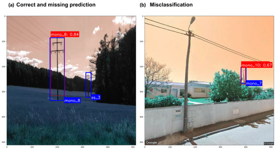
Figure 5.
Example of predictions returned by the object detection models trained to classify transmission towers. In blue, the ground truth bounding box, while in red, the bounding box of the prediction with the associated score.
The results are presented by firstly showcasing the performance of the object detection models on the two tasks previously introduced, i.e., identification and classification, on the test partition of the datasets, and thus, on images that the models never encountered during training. Secondly, the results of the prediction over the study area are presented, analyzing the spatial distribution of the accuracy of the prediction, along with a comparison between the two families of models used.
3.1. Identification
The identification was envisioned as the initial step into the investigation of the proposed methodology, since being able to recognize a tower in the image is seen as a preparatory step towards a better outcome in the classification phase. The confusion matrices in Figure 6 show a high accuracy in identifying towers for both models, with a slightly better performance given by the TSD. Notably, the upper row of the matrices is empty since the bounding boxes that correctly do not identify a tower are technically unbounded.
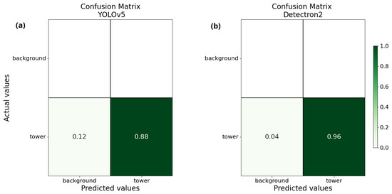
Figure 6.
Confusion matrices for the identification task. YOLOv5 on the left (a), Detectron2 on the right (b).
Figure 7 shows the precision-recall curves for the identification task for both the SSD model (YOLOv5) and the TSD model (Detectron2), along with their mean average precisions at an IoU of 0.5. The high values of mAP (83.67% for YOLOv5 and 88.64% for Detectron2) show the ability of both models in detecting and correctly placing the bounding box around the towers in the image, and similarly to the confusion matrices, it is observable how the TSD does slightly better than the SSD. Also, the high values of precision for increasing values of the recall demonstrate the ability of the models to recognize many relevant objects whilst identifying the majority of the towers. Nevertheless, it is noticeable how the two-stage detector is able to reach higher values of recall with respect to the single-stage detector, although with lower precision, highlighting the ability of the two-stage detector in detecting a larger portion of all possible towers recognizable in the picture.
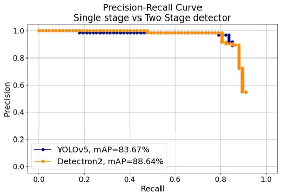
Figure 7.
Precision-recall curves and comparison of the mean average precisions for YOLOv5 and Detectron2 for the identification task.
Table 5 summarizes the metrics used to evaluate the models during the identification task. When looking at AP[0.5:0.05:0.95], and hence, the ability of the models to better localize the ground truth, although with a lower value, the disparity between TSD and SSD remains the same, showcasing that even averaging the mAP over different thresholds of IoU, Detectron2 still outperforms YOLOv5.
Table 5.
Summary of evaluation metrics for the identification task. The metrics are reported for the single-stage detector and the two-stage detector.
3.2. Classification
Regarding the performance of the models for the classification task, the confusion matrices can give a better understanding of how the predictions are spread among the 10 classes and give more insights into the misclassification. In Figure 8, it is possible to observe how the predictions behave for each class for the two models. Panels (a) and (c) display a good ability in recognizing the classes by the two models, evidenced by the prediction lying mostly along the diagonal. Looking at the first columns of the matrices, which highlight the false negatives (i.e., the models fail to predict a tower), the disparity between YOLOv5 and Detectron2 is rather evident, with the former having higher values (i.e., up to 0.4), and for all classes but one, and the latter lower values (i.e., up to 0.2), and for four classes of tower. In panels (b) and (d), the predictions are grouped by the family type of the transmission towers. Here, it is possible to observe that while the SSD indeed has more false negatives, it does a better job in predicting towers that belong to the actual family (i.e., maximum value of 0.03 for misclassifications for YOLOv5, and 0.09 for Detectron2).
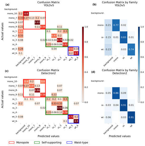
Figure 8.
Confusion matrices for the classification task. YOLOv5 in the top row, and Detectron2 on the bottom row. Panel (a,c) exhibit the confusion matrices for the 10 classes, while panels (b,d) show the confusion matrices grouped by family.
The confusion matrices allow the extraction of several metrics better equipped to synthesize the performance of the models. Table 6 shows, for each model, the F1-score, the precision, and the recall for each class. These metrics confirm the intuition provided by the confusion matrices. On average, Detectron2 achieves better results than YOLOv5, which is penalized by the higher number of false negatives as highlighted by the lower values of recall.
Table 6.
Metrics comparison for the classification task between YOLOv5 and Detectron2.
Table 7 reports the values of mAP for the ten tower classes at IoU = 0.5, while Figure 9 draws the mAP over the precision-recall plane for the same classes. It is observed that both models show a high mAP for most of the classes, with especially good performance for ss_3 and mono_8, which are among the most common types of towers and therefore might be easier to recognize. In terms of mAP over all the tower classes, a considerable difference is observed between SSD and TSD, which can be attributed in large portion to the poor performance of the YOLOv5 detector for two specific tower classes: the self-supporting single-level category and the monopole tubular single-level category (i.e., ss_1 and mono_7, respectively). The difference between the two type of models can be expected as shown in the literature, where studies compare these types of models.
Table 7.
Breakdown by class of the mean average precision for the classification task for the two types of models. The number of ground truth refers to the numerosity of each class in the images of the test partition. The symbol “#” denotes the numerosity, i.e., the number of items in the corresponding category.
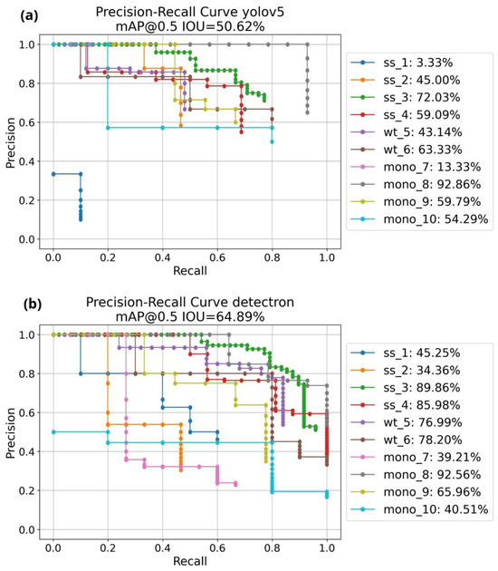
Figure 9.
Mean average precision for YOLOv5 (a) and Detectron2 (b) for the classification task. In the legend are reported the mean average precision for each class.
The relatively poor performance for these two tower classes might be due to a low number of samples in the training set and/or to the quality of the images used. Indeed, the dataset used to train the models might be inadequate to provide enough number of samples for the model to train on. However, this consideration might also point towards a higher robustness of the two-stage detector, where the sharp decrease for those classes is not observed. Indeed, without considering these two tower classes for the YOLOv5 model, the overall mAP would increase to an encouraging 61.2%, which would be closer to the performance provided by Detectron2 (i.e., 64.89%). It must be noted that, although the balance between the number of images for each class is important, in the real world, not all types of towers are employed at the same rate, and consequently, also finding images for each class to annotate is not a trivial task.
Table 8 summarizes the metrics regarding the classification task, where the advantage of Detectron2 is particularly visible in the classification task, as the difference in mAP never gets lower than 6%. Similarly to the identification task, the AP[0.5:0.05:0.95] metric confirms a better ability of the TSD to detect towers at varying IoUs than the SSD. The TSD decisively outperforms the SSD in every metric, showing a better ability in recognizing different object sizes in the image with increasing restricting IoU.
Table 8.
Summary of evaluation metrics for the identification task. The metrics are reported for the single-stage detector and the two-stage detector.
By analyzing the metrics adopted to evaluate the performance of the object detection models for the two tasks, a decrease in the performance is observed when going from the identification task to the classification task, which is somewhat expected. Moreover, in this case, this can be attributed mainly to two specific tower classes rather than the overall performance of the model, as previously discussed. Notwithstanding, the values obtained for the evaluation metrics are in line with other studies that use object detection models for customized tasks [56,57].
3.3. Spatial Distribution of the Predictions
The results presented up to now were obtained from the test partitioning of the two datasets. The application of the trained models to the whole study area is instead reported in Figure 10. Similarly to the testing set, the images of the whole study area were never seen before by the models, although in this case, the bounding boxes of the ground truth are not available for the entire area. This analysis allowed assessing how a given model would generalize in a real-life application. For the sake of brevity and clarity, the map shows the distribution of the confidence of the prediction (i.e., the level of confidence that the model has in recognizing a tower) over the entire study area only for the identification task. The points in light red are the towers for which the identification did not occur. The reasons for this might be multiple: (i) the model might not recognize any tower in the image, (ii) the image does not contain the tower because no available image of the tower is available, or (iii) the image of the tower might be obfuscated by an obstacle that was not taken into consideration in the proposed methodology (i.e., a truck parked on the side of the street, as well as a tree, could hide a clear shot of the transmission tower). Nevertheless, it is possible to see a large portion of dark blue points, which indicate the detection of towers with high levels of confidence (i.e., above 0.9). Still, the distribution of the dark blue area is not homogeneous. Both the northeast and southeast areas of the map show several towers that were not able to be identified. The missing predictions might be a consequence of the distance of the towers from the road and/or the morphology of the terrain. Another area where it is possible to notice a lower confidence in the predictions is close to the city of Porto. This might be expected due to the disturbance that the built environment inevitably brings to the images that are taken with Google Street View.
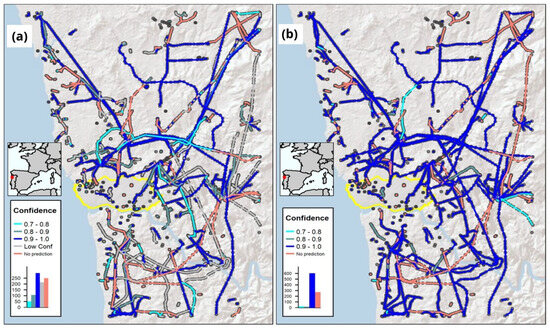
Figure 10.
Spatial distribution of the prediction confidence over the study area for the identification task performed by YOLOv5 (a) and Detectron2 (b).
Comparing the distribution of the confidence scores over the transmission tower’s lines, it is possible to identify areas where both models are unable to perform any predictions and lines where the TSD detector makes more confident predictions, or even performs predictions where the YOLOv5 model returns no prediction. In both maps, it is possible to observe that there were difficulties in making predictions in the north-east and, more generally, in the eastern side of the study area. As a matter of fact, those are regions that exhibit a complex orography in the form of mountainous areas, as well as areas that could be considered remote, and therefore reasonably away from roads that are covered by GSV imagery. In the southwest area of the map, the SSD model returns several missing predictions, whereas the TSD returns predictions with a high score. There are also important differences noticeable in the urban area of Porto, highlighted in yellow, where the low confidence predictions in Figure 10a are instead in the 0.9–1.0 range when looking at Figure 10b. Overall, the Detectron2 model returns a higher number of predictions with higher confidence than the YOLOv5 model, as can be seen in the histograms reported in the figures.
4. Conclusions
This study introduced a methodology to perform the automated classification of electrical transmission towers based on VGI data and street-level imagery, which is tested with two types of deep learning object detection models: a single-stage detector (i.e., YOLOv5) and a two-stage detector (i.e., Detectron2). The results showed that, in most cases, the deep learning models can identify towers in the images with a relatively high level of accuracy. This accuracy in the predictions decreases when the model is used to assign a class to the object, but the results remain comparable to those reported in related studies. The analysis also highlighted differences in performance between the two types of models. Overall, the TSD model outperformed the SSD model across most evaluation metrics and provided higher confidence scores. The outcomes of this work may contribute to large-scale risk assessment studies. The primary objective is to improve the exposure component of these assessments, which often employ methods that do not make full use of the growing availability of user-generated content. Enhancing the capacity to utilize such data may improve the accuracy and utility of large-scale risk evaluations related to natural hazards.
The proposed methodology, however, has some limitations that could be addressed in future work. These can be grouped into two main categories: those related to technological constraints and those inherent to the nature of the methodology and its subject. Regarding the latter, because power grids are distributed across various terrains and not always close to roads, it is often difficult to capture clear images of towers located at greater distances. This situation increases the likelihood of visual obstructions. In urban areas, occlusion by buildings is a common issue, particularly in densely built environments. Although the use of geometric and elevation-based heuristics to filter obstructed GSV images is a significant methodological strength, explicitly quantifying its positive impact on the quality of the final dataset could improve the robustness of the approach and provide insights on how to further refine it. Regarding technological constraints, limitations imposed by image providers such as Google Street View present additional challenges. The image quality is not consistent with the capabilities of the imaging instruments used, which typically produce higher-resolution data. Additionally, metadata about the camera or the original image size in pixels is not available, making it difficult to derive important information such as the height of the towers. Moreover, the size of the datasets and the number of samples per class influence the training process and, consequently, model performance. Collecting and annotating images is a resource-intensive task, especially given the specific nature of the problem. While automated collection remains complex due to the need for images of particular types of towers, annotation could potentially be supported through unsupervised algorithms to facilitate the construction of larger training datasets.
In response to these challenges, several complementary strategies could be explored to improve data quality and coverage. Data augmentation techniques, as well as the use of drone-based or LiDAR imagery, may help address issues related to dataset size and class imbalance. These approaches would not only expand the volume and diversity of available data but also offer imagery that is free from the usage restrictions imposed by the Terms of Services of street-level imagery providers. Furthermore, such alternatives may help mitigate concerns related to privacy, intellectual property, and the underrepresentation of certain geographic or socioeconomic areas. In addition, there are also possible refinements that can be made to the model architecture. For example, the integration of additional layers may enhance performance, though this may come at the cost of increased training and detection time, which may be acceptable in this context, where real-time processing is not a requirement. Similarly, implementing attention mechanisms or alternative padding techniques designed to optimize information extraction from input images could improve model performance, as suggested by [58]. In summary, the present study presents an initial step toward the application of the proposed methodology for natural hazard risk assessment and supports future developments aimed at constructing large-scale exposure datasets with improved detail. Furthermore, the methodological framework remains relevant and applicable with newer model versions as they continue to come out in the future.
Author Contributions
Conceptualization, L.C., R.F. and X.R.; methodology, L.C., R.F., X.R. and M.M.; software, L.C.; investigation, L.C., R.F., X.R. and M.M.; data curation, L.C.; writing—original draft preparation, L.C. and R.F.; writing—review and editing, L.C., R.F., X.R. and M.M.; supervision, R.F. and M.M. All authors have read and agreed to the published version of the manuscript.
Funding
This work was financially supported by the Portuguese Foundation for Science and Technology through the CEEC programme (2022.03980.CEECIND/CP1728/CT0003); the Italian Ministry of Education, within the framework of the project Dipartimenti di Eccellenza at IUSS Pavia; the Regione Lombardia within the framework of the project IUSS Data Center (DGR n.XI/3776/2020); Funding—UID/04708 of the CONSTRUCT—Instituto de I&D em Estruturas e Construçõ—funded by Fundação para a Ciência e a Tecnologia, I.P./MCTES through the national funds.
Data Availability Statement
The datasets regarding the annotated images of towers, and the codes developed in this study are available at the following link https://github.com/luigicesarini/ExposureModellingTower (accessed on 19 June 2025).
Conflicts of Interest
The authors declare no conflicts of interest.
Abbreviations
The following abbreviations are used in this manuscript:
| GSV | Google Street View |
| OSM | Open Street Map |
| YOLOv5 | You Only Look Once version 5 |
| API | Application Programming Interface |
| JSON | JavaScript Object Notation |
| UAV | Unmanned Aerial Vehicle |
| mAP | Mean average precision |
| SRTM | Shuttle Radar Topography Mission |
| SSD | Single-stage detector |
| TSD | Two-stage detector |
| AP | Average precision |
| IoU | Intersection over Union |
| ML | Machine Learning |
| DL | Deep Learning |
| VGI | Volunteered Geographic Information |
| FPN | Feature Pyramid Network |
| RPN | Region Proposal Network |
| RoI | Region of Interest |
| TP | True Positive |
| FP | False Positive |
| FN | False Negative |
| TN | True Negative |
| P | Precision |
| R | Recall |
Appendix A. Equation for Deriving the Optimal Google Street-View Parameters
Here are reported the equations used to derive the optimal parameters for querying GSV imagery. An implementation of these equations can be found at the link of the repository.
Knowing the position (longitude, latitude) of the towers and the positions (longitude, latitude) of the closest GSV, it is possible to compute the distances (D) Equation (A1), and the difference in elevations () Equation (A2).
Once the distances and differences in elevation are obtained, the parameters needed for the GSV query, namely, heading Equation (A3), field of view Equation (A4), and pitch Equation (A5), can be computed as follows:
where a and b are the coefficients of the line between the points with distance 10 m and field of view 90 and 600 m and field of view 15, respectively.
References
- IPCC. Summary for Policymakers. In Climate Change 2022: Impacts, Adaptation and Vulnerability; Pörtner, H.-O., Roberts, D.C., Poloczanska, E.S., Mintenbeck, K., Tignor, M., Alegría, A., Craig, M., Langsdorf, S., Löschke, S., Möller, V., et al., Eds.; Cambridge University Press: Cambridge, UK, 2021. [Google Scholar] [CrossRef]
- Figueiredo, R.; Martina, M. Using open building data in the development of exposure data sets for catastrophe risk modelling. Nat. Hazards Earth Syst. Sci. 2016, 16, 417–429. [Google Scholar] [CrossRef]
- Pearson, L.; Pelling, M. The UN Sendai Framework for Disaster Risk Reduction 2015–2030: Negotiation Process and Prospects for Science and Practice. J. Extrem. Events 2015, 02, 1571001. [Google Scholar] [CrossRef]
- Wieland, M.; Pittore, M.; Parolai, S.; Zschau, J.; Moldobekov, B.; Begaliev, U. Estimating building inventory for rapid seismic vulnerability assessment: Towards an integrated approach based on multi-source imaging. Soil Dyn. Earthq. Eng. 2012, 36, 70–83. [Google Scholar] [CrossRef]
- De Albuquerque, J.P.; Herfort, B.; Brenning, A.; Zipf, A. A geographic approach for combining social media and authoritative data towards identifying useful information for disaster management. Int. J. Geogr. Inf. Sci. 2015, 29, 667–689. [Google Scholar] [CrossRef]
- Klonner, C.; Marx, S.; Usón, T.; Porto de Albuquerque, J.; Höfle, B. Volunteered Geographic Information in Natural Hazard Analysis: A Systematic Literature Review of Current Approaches with a Focus on Preparedness and Mitigation. ISPRS Int. J. Geo-Inf. 2016, 5, 103. [Google Scholar] [CrossRef]
- LeCun, Y.; Bengio, Y.; Hinton, G. Deep learning. Nature 2015, 521, 436–444. [Google Scholar] [CrossRef]
- Geiß, C.; Schauß, A.; Riedlinger, T.; Dech, S.; Zelaya, C.; Guzmán, N.; Hube, M.A.; Arsanjani, J.J.; Taubenböck, H. Joint use of remote sensing data and volunteered geographic information for exposure estimation: Evidence from Valparaíso, Chile. Nat. Hazards 2017, 86, 81–105. [Google Scholar] [CrossRef]
- Aravena Pelizari, P.; Geiß, C.; Aguirre, P.; Santa María, H.; Merino Peña, Y.; Taubenböck, H. Automated building characterization for seismic risk assessment using street-level imagery and deep learning. ISPRS J. Photogramm. Remote Sens. 2021, 180, 370–386. [Google Scholar] [CrossRef]
- Xu, J.Z.; Lu, W.; Li, Z.; Khaitan, P.; Zaytseva, V. Building Damage Detection in Satellite Imagery Using Convolutional Neural Networks. arXiv 2019, arXiv:1910.06444. [Google Scholar]
- Iannelli, G.; Dell’Acqua, F. Extensive Exposure Mapping in Urban Areas through Deep Analysis of Street-Level Pictures for Floor Count Determination. Urban Sci. 2017, 1, 16. [Google Scholar] [CrossRef]
- Fujita, S.; Hatayama, M. Estimation Method for Roof-damaged Buildings from Aero-Photo Images During Earthquakes Using Deep Learning. Inf. Syst. Front. 2021, 25, 351–363. [Google Scholar] [CrossRef]
- Hu, Z.; He, T.; Zeng, Y.; Luo, X.; Wang, J.; Huang, S.; Liang, J.; Sun, Q.; Xu, H.; Lin, B. Fast image recognition of transmission tower based on big data. Prot. Control Mod. Power Syst. 2018, 3, 15. [Google Scholar] [CrossRef]
- Wang, H.; Yang, G.; Li, E.; Tian, Y.; Zhao, M.; Liang, Z. High-Voltage Power Transmission Tower Detection Based on Faster R-CNN and YOLO-V3. In Proceedings of the 2019 Chinese Control Conference (CCC), Guangzhou, China, 27–30 July 2019; pp. 8750–8755. [Google Scholar] [CrossRef]
- Pescaroli, G.; Alexander, D. Critical infrastructure, panarchies and the vulnerability paths of cascading disasters. Nat. Hazards 2016, 82, 175–192. [Google Scholar] [CrossRef]
- Bhusal, N.; Abdelmalak, M.; Kamruzzaman, M.; Benidris, M. Power System Resilience: Current Practices, Challenges, and Future Directions. IEEE Access 2020, 8, 18064–18086. [Google Scholar] [CrossRef]
- López, A.L.; Rocha, L.E.P.; Escobedo, D.d.L.; Sánchez, J. Reliability and Vulnerability Analysis of Electrical Substations and Transmission Towers for Definition of Wind and Seismic Damage Maps for Mexico. In Proceedings of the 11th Americas Conference on Wind Engineering, San Juan, Puerto Rico, 22–26 June 2009; p. 13. [Google Scholar]
- Rezaei, S.N.; Chouinard, L.; Legeron, F.; Langlois, S. Vulnerability Analysis of Transmission Towers subjected to Unbalanced Ice Loads. In Proceedings of the 112th International Conference on Applications of Statistics and Probability in Civil Engineering, ICASP12, Vancouver, BC, Canada, 12–15 July 2015; p. 8. [Google Scholar]
- Tapia-Hernández, E.; De-León-Escobedo, D. Vulnerability of transmission towers under intense wind loads. Struct. Infrastruct. Eng. 2021, 18, 1235–1250. [Google Scholar] [CrossRef]
- Minghini, M.; Sarretta, A.; Napolitano, M. OpenStreetMap Contribution to Local Data Ecosystems in COVID-19 Times: Experiences and Reflections from the Italian Case. Data 2022, 7, 39. [Google Scholar] [CrossRef]
- Contributors, O. Stats—OpenStreetMap Wiki. 2024. Available online: https://wiki.openstreetmap.org/wiki/Stats (accessed on 1 June 2025).
- Contributors, O. Elements—OpenStreetMap Wiki. 2024. Available online: https://wiki.openstreetmap.org/wiki/Elements (accessed on 1 June 2025).
- OpenStreetMap Contributors. List of OSM-Based Services—OpenStreetMap Wiki. 2024. Available online: https://wiki.openstreetmap.org/wiki/List_of_OSM-based_services (accessed on 10 May 2024).
- Alvarez Leon, L.; Quinn, S. Street-level Imagery. In The Geographic Information Science & Technology Body of Knowledge; University Consortium for Geographic Information Science: Chesapeake, VA, USA, 2019. [Google Scholar] [CrossRef]
- Anguelov, D.; Dulong, C.; Filip, D.; Frueh, C.; Lafon, S.; Lyon, R.; Ogale, A.; Vincent, L.; Weaver, J. Google Street View: Capturing the World at Street Level. Computer 2010, 43, 32–38. [Google Scholar] [CrossRef]
- Zou, S.; Wang, L. Detecting individual abandoned houses from google street view: A hierarchical deep learning approach. ISPRS J. Photogramm. Remote Sens. 2021, 175, 298–310. [Google Scholar] [CrossRef]
- Google. Panoramica dell’API Street View Static|Street View Static API. July 2024. Available online: https://developers.google.com/maps/documentation/streetview/overview?hl=it (accessed on 11 June 2024).
- Everingham, M.; Van Gool, L.; Williams, C.K.I.; Winn, J.; Zisserman, A. The Pascal Visual Object Classes (VOC) Challenge. Int. J. Comput. Vis. 2010, 88, 303–338. [Google Scholar] [CrossRef]
- Lin, T.Y.; Maire, M.; Belongie, S.; Bourdev, L.; Girshick, R.; Hays, J.; Perona, P.; Ramanan, D.; Zitnick, C.L.; Dollár, P. Microsoft COCO: Common Objects in Context. arXiv 2015, arXiv:1405.0312. [Google Scholar]
- Chiu, M.T.; Xu, X.; Wei, Y.; Huang, Z.; Schwing, A.G.; Brunner, R.; Khachatrian, H.; Karapetyan, H.; Dozier, I.; Rose, G.; et al. Agriculture-Vision: A Large Aerial Image Database for Agricultural Pattern Analysis. In Proceedings of the 2020 IEEE/CVF Conference on Computer Vision and Pattern Recognition (CVPR), Seattle, WA, USA, 13–19 June 2020; pp. 2825–2835. [Google Scholar] [CrossRef]
- Preeti, C.; Mohan, K.J. Analysis of transmission towers with different configurations. Jordan J. Civ. Eng. 2013, 7, 450–460. [Google Scholar]
- Paiva, F.; Henriques, J.; Barros, R.C. Review of transmission tower testing stations around the world. Procedia Eng. 2013, 57, 859–868. [Google Scholar] [CrossRef][Green Version]
- Tibolt, M.; Bezas, M.; Vayas, I.; Jaspart, J. The design of a steel lattice transmission tower in Central Europe. ce/papers 2021, 4, 243–248. [Google Scholar] [CrossRef]
- Stracqualursi, E.; Pelliccione, G.; Celozzi, S.; Araneo, R. Tower models for power systems transients: A review. Energies 2022, 15, 4893. [Google Scholar] [CrossRef]
- Marin-Castro, H.; Sucar, E.; Morales, E. Automatic Image Annotation Using a Semi-supervised Ensemble of Classifiers. In Progress in Pattern Recognition, Image Analysis and Applications; Rueda, L., Mery, D., Kittler, J., Eds.; Springer: Berlin/Heidelberg, Germany, 2008; Volume 4756, pp. 487–495. [Google Scholar] [CrossRef]
- Ratner, A.; Bach, S.H.; Ehrenberg, H.; Fries, J.; Wu, S.; Ré, C. Snorkel: Rapid training data creation with weak supervision. VLDB J. 2020, 29, 709–730. [Google Scholar] [CrossRef]
- Shahinfar, S.; Meek, P.; Falzon, G. “How many images do I need?” Understanding how sample size per class affects deep learning model performance metrics for balanced designs in autonomous wildlife monitoring. Ecol. Inform. 2020, 57, 101085. [Google Scholar] [CrossRef]
- Nguyen, V.N.; Jenssen, R.; Roverso, D. Intelligent Monitoring and Inspection of Power Line Components Powered by UAVs and Deep Learning. IEEE Power Energy Technol. Syst. J. 2019, 6, 11–21. [Google Scholar] [CrossRef]
- Hui, X.; Bian, J.; Zhao, X.; Tan, M. Vision-based autonomous navigation approach for unmanned aerial vehicle transmission-line inspection. Int. J. Adv. Robot. Syst. 2018, 15, 172988141775282. [Google Scholar] [CrossRef]
- Zhang, S.; Benenson, R.; Omran, M.; Hosang, J.; Schiele, B. How Far are We from Solving Pedestrian Detection? In Proceedings of the 2016 IEEE Conference on Computer Vision and Pattern Recognition (CVPR), Las Vegas, NV, USA, 27–30 June 2016; pp. 1259–1267. [Google Scholar] [CrossRef]
- Olivier, A.; Raynaud, C. Balanced sampling for an object detection problem—Application to fetal anatomies detection. In Proceedings of the Medical Imaging with Deep Learning, Lübeck, Germany, 7 July 2021; p. 13. [Google Scholar]
- Reitermanova, Z. Data splitting. In Proceedings of the WDS’10 Proceedings of Contributed Papers-WDS 2010; Prague, Czech Republic, 1–4 June 2010, Volume 10, pp. 31–36.
- Muhammad, A.R.; Utomo, H.P.; Hidayatullah, P.; Syakrani, N. Early Stopping Effectiveness for YOLOv4. J. Inf. Syst. Eng. Bus. Intell. 2022, 8, 29988. [Google Scholar] [CrossRef]
- Sultana, F.; Sufian, A.; Dutta, P. A Review of Object Detection Models Based on Convolutional Neural Network. In Intelligent Computing: Image Processing Based Applications; Mandal, J.K., Banerjee, S., Eds.; Advances in Intelligent Systems and Computing; Springer: Singapore, 2020; Volume 1157, pp. 1–16. [Google Scholar] [CrossRef]
- Wu, Y.; Kirillov, A.; Massa, F.; Lo, W.Y.; Girshick, R. Detectron2. 2019. Available online: https://github.com/facebookresearch/detectron2 (accessed on 1 June 2025).
- Jocher, G.; Stoken, A.; Chaurasia, A.; Borovec, J.; NanoCode012; TaoXie; Kwon, Y.; Michael, K.; Changyu, L.; Fang, J.; et al. ultralytics/yolov5: V6.0-YOLOv5n ’Nano’ Models, Roboflow Integration, TensorFlow Export, OpenCV DNN Support. 2021; Available online: https://zenodo.org/records/5563715 (accessed on 22 June 2025).
- Lin, T.Y.; Dollár, P.; Girshick, R.; He, K.; Hariharan, B.; Belongie, S. Feature Pyramid Networks for Object Detection. arXiv 2016, arXiv:1612.03144. [Google Scholar] [CrossRef]
- Ren, S.; He, K.; Girshick, R.; Sun, J. Faster R-CNN: Towards Real-Time Object Detection with Region Proposal Networks. In Proceedings of the Advances in Neural Information Processing Systems; Cortes, C., Lawrence, N., Lee, D., Sugiyama, M., Garnett, R., Eds.; Curran Associates, Inc.: San Diego, CA, USA, 2015; Volume 28. [Google Scholar]
- Redmon, J.; Divvala, S.; Girshick, R.; Farhadi, A. You Only Look Once: Unified, Real-Time Object Detection. arXiv 2016, arXiv:1506.02640. [Google Scholar]
- Soviany, P.; Ionescu, R.T. Optimizing the Trade-off between Single-Stage and Two-Stage Object Detectors using Image Difficulty Prediction. arXiv 2018, arXiv:1803.08707. [Google Scholar]
- Lu, X.; Li, Q.; Li, B.; Yan, J. MimicDet: Bridging the Gap Between One-Stage and Two-Stage Object Detection. In Computer Vision—ECCV 2020; Vedaldi, A., Bischof, H., Brox, T., Frahm, J.M., Eds.; Lecture Notes in Computer Science; Springer International Publishing: Cham, Switzerland, 2020; Volume 12359, pp. 541–557. [Google Scholar] [CrossRef]
- Padilla, R.; Passos, W.L.; Dias, T.L.B.; Netto, S.L.; Da Silva, E.A.B. A Comparative Analysis of Object Detection Metrics with a Companion Open-Source Toolkit. Electronics 2021, 10, 279. [Google Scholar] [CrossRef]
- Stehman, S.V. Selecting and interpreting measures of thematic classification accuracy. Remote Sens. Environ. 1997, 62, 77–89. [Google Scholar] [CrossRef]
- Ivchenko, G.I.; Honov, S.A. On the jaccard similarity test. J. Math. Sci. 1998, 88, 789–794. [Google Scholar] [CrossRef]
- Saito, T.; Rehmsmeier, M. The Precision-Recall Plot Is More Informative than the ROC Plot When Evaluating Binary Classifiers on Imbalanced Datasets. PLoS ONE 2015, 10, e0118432. [Google Scholar] [CrossRef]
- Abdelfattah, R.; Wang, X.; Wang, S. TTPLA: An Aerial-Image Dataset for Detection and Segmentation of Transmission Towers and Power Lines. arXiv 2020, arXiv:2010.10032. [Google Scholar]
- Mittal, P.; Singh, R.; Sharma, A. Deep learning-based object detection in low-altitude UAV datasets: A survey. Image Vis. Comput. 2020, 104, 104046. [Google Scholar] [CrossRef]
- Zhu, L.; Geng, X.; Li, Z.; Liu, C. Improving YOLOv5 with Attention Mechanism for Detecting Boulders from Planetary Images. Remote Sens. 2021, 13, 3776. [Google Scholar] [CrossRef]


Disclaimer/Publisher’s Note: The statements, opinions and data contained in all publications are solely those of the individual author(s) and contributor(s) and not of MDPI and/or the editor(s). MDPI and/or the editor(s) disclaim responsibility for any injury to people or property resulting from any ideas, methods, instructions or products referred to in the content. |
© 2025 by the authors. Licensee MDPI, Basel, Switzerland. This article is an open access article distributed under the terms and conditions of the Creative Commons Attribution (CC BY) license (https://creativecommons.org/licenses/by/4.0/).