Abstract
Deflection slopes measured by the traffic speed deflectometer (TSD) are being used to backcalculate the moduli of pavement layers. Pavement surface roughness causes variations in tyre load magnitude due to excitation, which affects TSD measurements. In this study, three rough pavement surface profiles over 150 m longitudinal distances were extracted from the Long-Term Pavement Performance (LTPP) programme database. Utilising finite element method (FEM) simulation of the TSD pass at a travel speed of 80 km/h over a three-layer flexible pavement system containing the rough surface profiles and employing the Greenwood Engineering TSD backcalculation tool, it was found that tyre load excitation can lead to backcalculation errors of up to 48%. By obtaining deflection slopes at equal distance intervals along the 150 m pavement profiles, it was found that averaging the deflection slopes across 9 measurement points reduced backcalculation errors to 10%, while increasing the number of measurement points to 28 further lowered the backcalculation errors to 5%. These findings highlight the potential to mitigate the effects of tyre load excitation on TSD backcalculation outputs without relying on strain gauges, which are mounted on modern TSDs to measure instantaneous tyre load magnitudes but are sensitive to environmental conditions and require calibration.
1. Introduction
The falling weight deflectometer (FWD) is a widely used tool for assessing the structural condition of pavement systems. However, due to its stationary nature and the requirement to close lanes during testing, its use is limited to project-level evaluations [1]. To address the limitations of the FWD, a number of mobile devices capable of operating at traffic speed have been developed in the US and Europe. One such device is the traffic speed deflectometer (TSD) [2]. The TSD measures pavement deflection velocities on one side of the rear axle using Doppler laser sensors. These velocities are then normalised by the travel speed to obtain deflection slopes [3]. Several applications for TSD measurements in pavement management have been proposed in previous studies, such as evaluating the remaining service life of motorway pavements [4], predicting critical strains in flexible pavement systems [5], determining the structural number (SN) of existing pavements [6], and measuring joint displacement in rigid pavements to evaluate load transfer efficiency (LTE) [7].
Another major application of TSD measurements, which has been widely investigated in previous studies, is backcalculating the moduli of flexible pavement layers. In the velocity and deflection backcalculation methods developed by Nasimifar et al. [8], as well as the viscoelastic backcalculation approach proposed by Nielsen [9], a TSD moving load with a constant load magnitude was assumed. However, when a vehicle drives on a rough road, it can cause dynamic excitations that lead to the pavement experiencing heavier loads from the vehicle [10]. The dynamic load coefficient (DLC), a dimensionless parameter, emerges by dividing the standard deviation of dynamic load by the mean static load. Through the application of DLC, it becomes feasible to ascertain the probabilistic extent of the dynamic axle load based on vehicle speed, vehicle suspension system, and road surface roughness. Ideally, a truck moving over a smooth road would exhibit a DLC value approaching zero [11]. The consideration of DLC into a backcalculation approach has been explored by correlating FWD and TSD deflections obtained from the 3D-Move programme [12] using an artificial neural network (ANN), with the aim of enabling the use of correlated TSD deflections as input for FWD backcalculation tools [13]. By incorporating the DLC parameter, the influence of variations in dynamic load magnitude caused by pavement surface roughness on backcalculated moduli has been investigated using an iterative approach employing the constrained extended Kalman filter (CEKF) within a two-and-a-half-dimensional (2.5D) finite element method (FEM). It was found that when the DLC for tyre load magnitude varied from 0.7 to 1.3, it could lead to errors of up to 30% in the backcalculated moduli of the pavement layers [14]. Instead of considering DLC in dynamic load variations, TSD dynamic loading data was obtained using TruckSim software [15] based on the surface profile of a specific pavement section. The semi-analytical finite element method (SAFEM) was then used to model the TSD dynamic loading at a specified travel speed to assess its impact on deflection values and deflection slopes [16].
Two major types of uncertainties exist when modelling real world events. Aleatoric or data uncertainty refers to the inherent randomness and noise in the data entered into the model, while epistemic or model uncertainty arises from limited knowledge or specific assumptions made in the model [17]. With regard to TSD data uncertainty, TSD measurements may be affected by noise in the raw data [18] or by sources of randomness such as spatial variations in pavement structure [19] and changes in dynamic load magnitude caused by pavement surface roughness. As discussed earlier, changes in dynamic load magnitude influence deflection slopes and affect the backcalculated moduli derived from them. Some backcalculation techniques do not account for variations in dynamic load in TSDs, while others incorporate these changes into their approaches and analyses. Quantitative techniques such as averaging deflection slopes over different travel lengths have been proposed in previous studies to reduce random noise in TSD data while preserving the part of the signal related to spatial variations in pavement structure, and these methods are discussed in the next section [18,19,20,21,22]. However, the mitigation of randomness in TSD measurements caused by dynamic load excitation from pavement surface roughness has not been discussed in previous studies. Modern TSDs are equipped with strain gauges on their rear axles to measure the strain applied, enabling continuous measurement of dynamic load magnitudes [23,24]. However, strain gauges require calibration, and their performance is highly sensitive to environmental factors such as temperature and humidity, which can compromise the reliability of the measurements [25]. Therefore, it would be highly valuable to investigate whether averaging TSD measurements for the purpose of data noise removal contributes to reducing the data randomness caused by changes in dynamic load magnitude influenced by pavement surface roughness. Through this evaluation, it can be determined whether the averaging process could eliminate the need for instantaneous load measurements from strain gauges, specifically for backcalculation purposes, since such instrumentation increases setup and maintenance costs. This investigation can be carried out through finite element simulation of flexible pavement systems.
2. Processing of TSD Raw Data Measurements
TSD devices measure raw deflection velocities at around 1000 Hz, but the collected data contain considerable random noise. Averaging over specific travel-length intervals as a quantitative approach can help reduce this noise; however, when the averaging length is too small, the noise may still be noticeable. Consequently, in the UK, TSD measurements are averaged over 10-metre intervals, while the raw data are collected at 1-metre intervals. It should be noted that this noise-reduction technique may not reveal actual variations in TSD deflections [18]. Figure 1 illustrates the raw deflection velocities measured at 1-metre chainage intervals by the Doppler laser sensor positioned at 300 mm offset distance from the centre of loading, obtained during a TSD field evaluation conducted on the Roskilde Loop in Denmark.
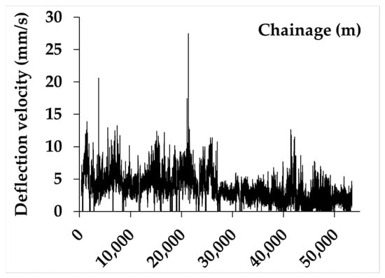
Figure 1.
A sample of raw TSD measurements at Roskilde Loop in Denmark.
More advanced techniques have been proposed to remove TSD signal noise without relying solely on averaging the measurements over fixed lengths. Given the likely spatial variability in pavement structure during TSD evaluations, it is important to apply a noise reduction technique that retains the parts of the signal related to spatial changes. By recognising the normal distribution characteristics of TSD measurement errors, the use of weighted averaging through smoothing spline regression, achieved by minimising the generalised cross-validation (GCV) criterion for optimal smoothing, has been shown to be a practical method for TSD data denoising [19]. Wavelet-based denoising has also been proposed to remove noise from TSD deflection slopes, with three different wavelet approaches suggested, each suitable for either project-level or network-level pavement management [20]. An additional attempt to optimise the averaging of TSD measurements for noise reduction used the difference sequence method to calculate the standard deviations of noise and the true signal, which reflects structural variations within the pavement system. When compared with the results obtained from the GCV-based smoothing method, the difference sequence method was found to be more effective [21]. More recently, a TSD signal denoising approach based on variational mode decomposition (VMD), combined with the particle swarm optimisation (PSO) algorithm, has been proposed and shown to be effective in eliminating noise from TSD data [22].
3. International Roughness Index (IRI)
Irregularities in the road surface induce oscillations in the wheels of vehicles, and these oscillations are subsequently conveyed to the loading axles. The suspension system of the vehicle plays a crucial role in mitigating the vibrations transmitted to the car body. Vehicles employ three distinct categories of suspension systems: passive, semi-active, and active. Passive systems are the most prevalent [26]. They comprise an element for dissipating energy (a damper) and an element for storing energy (a spring) without the capability to introduce additional energy into the system [27].
The International Roughness Index (IRI) serves as the universally accepted standard for measuring pavement surface roughness and has gained widespread popularity as the most frequently employed index for this purpose [28]. IRI is calculated in units of m/km based on the response of a quarter-car model, referred to as the golden car, travelling at a speed of 80 km/h utilising the passive suspension system [29]. IRI exhibits a linear relationship with surface roughness, implying that a certain percentage increase in elevation values within a measured profile leads to an equivalent percentage increase in the IRI. A perfect flat profile is denoted by an IRI value of zero. Table 1 illustrates the types of pavements based on their roughness levels and provides the IRI index range for each category [30].

Table 1.
IRI range corresponding to pavement surface roughness levels (data from [30]).
Figure 2 illustrates the physical representation of the golden car’s suspension system elements, with detailed description of each element provided at the bottom of the figure [31]. The model’s differential equations of motion are presented in Equations (1) and (2), with the matrix form depicted in Equation (3) [32]. It is important to note, as depicted in Equation (3), that the ratios of masses and the constants of springs and dampers play a crucial role in solving the equation. These ratios are specifically provided for the golden car’s suspension system, as illustrated in Table 2 [33].
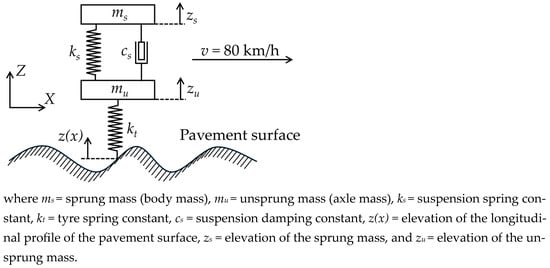
Figure 2.
Golden car’s suspension system elements.

Table 2.
Parameters ratios in the golden car’s suspension system (data from [33]).
After solving the system of differential equations presented in Equations (1)–(3), the IRI can be calculated using Equation (4) [32]. As depicted in Figure 2, it is evident that at each instant, the force magnitude applied to the ground surface corresponds to the force in the tyre spring. By dividing this force by the total mass of the suspension system, the vertical acceleration, denoted by av, applied to the vehicle by the pavement surface can be calculated using Equation (5).
where l = distance travelled by the vehicle, v = travel speed, and t = travel time.
4. Greenwood Engineering TSD Backcalculation Tool
Greenwood Engineering has developed a backcalculation tool for its TSD users worldwide. The tool runs on a web service platform [34] and provides the backcalculated moduli of pavement layers directly from the measured deflection slopes. It uses inputs such as the weights of the TSD truck and trailer axles, the thicknesses of pavement layers obtained using ground-penetrating radar (GPR) during TSD evaluation [35], and the Poisson’s ratios of the pavement layers. The tool can account for both linear elastic behaviour and the time dependent or viscoelastic behaviour of pavement materials. If the user chooses to ignore time dependency and viscoelasticity, the tool provides a linear elastic modulus as the backcalculation output for each layer. The tool was developed based on a previous study [9] and follows the same assumptions. These include a uniform density of 2000 kg/m3 for all pavement layers, an equivalent dual circular loading area on each side of the loading axles with a dual wheel spacing of 350 mm and an axle width of 1820 mm, and a truck-to-trailer axle distance of 8150 mm. A uniform tyre contact pressure of 0.85 MPa is considered to apply across all wheels during the backcalculation process.
5. Effect of Vertical Acceleration on Tyre Load Magnitude
Figure 3 shows a diagram of the vertical forces on a tyre travelling over a pavement system, focusing on the effect of pavement surface roughness and neglecting other forces such as tyre–pavement friction.
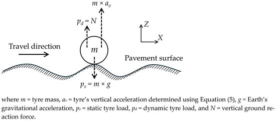
Figure 3.
Vertical loads applied on a tyre travelling over a pavement system.
It should be noted that the dynamic tyre load is equal to the vertical reaction force exerted on the tyre by the pavement surface. Consequently, as shown in Figure 3, pd is equal to N. When the vehicle travels over a perfectly smooth pavement surface and no vertical acceleration arises from surface roughness, the dynamic tyre load becomes equal to the static tyre load, ensuring equilibrium of forces in the vertical direction.
Assuming a circular contact area as adopted in the Greenwood Engineering backcalculation tool, Equation (6) shows the relationship between the static tyre load, the tyre contact pressure, and the static loading radius. Referring to the diagram in Figure 3, Equation (7) describes the relationship between static and dynamic tyre loads. By substituting the dynamic tyre load from Equation (7) into Equation (6), the equivalent dynamic circular loading radius, which accounts for the effect of pavement surface roughness on the dynamic tyre load, can be calculated using Equation (8).
where q = tyre contact pressure, and as = equivalent circular loading radius in static loading.
where ad = equivalent circular loading radius in dynamic loading.
It should be noted that based on the load directions shown in Figure 3, av in Equation (8) is obtained as positive when the effect of pavement surface roughness opposes the tyre’s static weight, which occurs under tyre load attenuation. In contrast, av is negative when pavement surface roughness intensifies the tyre’s static load, which corresponds to tyre load amplification.
6. Materials and Methods
Figure 4 presents an overall flowchart of the methodology adopted in this study. Three distinct rough pavement surface elevation profiles, each spanning 150 m in length, were extracted from the Long-Term Pavement Performance (LTPP) Programme Standard Data Release (SDR) database [36]. The IRI values of the surface profiles were 2.77, 3.04, and 3.18 m/km, corresponding to surveys conducted in the states of Texas (TX), Pennsylvania (PA), and Minnesota (MN), respectively. Table 3 presents the details of each surface profile survey. Rough pavement surface profiles were selected, as they have a stronger effect on the DLC and the magnitudes of attenuated and amplified tyre loads caused by surface roughness [37]. The system of ordinary differential equations (ODEs) presented in Equation (3) for the golden car travel was solved numerically using MATLAB R2022b’s ODE45 solver [38], with the results input into Equation (5) to calculate tyre vertical accelerations along three surface profiles. This analysis identified two key locations on each profile where the highest attenuation and the highest amplification of tyre load magnitude occurred due to the effect of pavement surface roughness. For each of the points showing the highest attenuation and highest amplification on each of the three surface profiles, ten auxiliary point sets were defined, each having longitudinal point intervals of 2.5, 5, 10, 15, 20, 25, 30, 40, 50, or 60 m. As an example, Figure 5 illustrates a schematic of the points with the highest attenuation and amplification, along with their corresponding 15 m interval auxiliary point sets. Subsequently, the tyre vertical acceleration at each point in every point set was calculated by using Equation (5). The rear axle of a TSD was then simulated in three-dimensional (3D) ABAQUS [39] using the FEM as it travelled over a three-layer flexible pavement system. The dynamic load magnitude used in each FEM simulation was determined by decoupling vehicle vibration from pavement surface roughness and was calculated based on the tyre vertical acceleration previously obtained for the points with the highest attenuation and the highest amplification, along with their associated auxiliary points in each point set. Afterwards, deflection slopes were calculated at various offset distances from the centre of loading on the side equipped with Doppler laser sensors. These deflection slopes were entered into the Greenwood Engineering TSD backcalculation tool, either directly for each highest attenuation and highest amplification point or by averaging the deflection slopes of each highest attenuation and amplification point together with their corresponding auxiliary points in each point set. The backcalculated moduli of the pavement layers were then obtained.
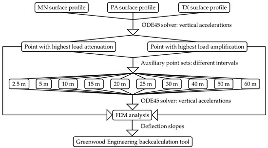
Figure 4.
Flowchart depicting overall methodology of current study.

Table 3.
Details of pavement surface profile surveys (data from [36]).
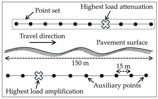
Figure 5.
Schematic of the points with highest attenuation and amplification and 15 m interval points (not to scale).
It should be noted that, since tyre vertical accelerations from the golden car suspension system’s equations of motion were used in the FEM, the TSD vehicle was assumed to have the same suspension system as the golden car. The TSD travel speed was set to 80 km/h, as higher speeds have a greater impact on the DLC [40] and, therefore, a more pronounced effect on the vertical accelerations caused by pavement surface roughness. Further details of the FEM simulations and calculations carried out in this study are provided in the following subsections.
It is also important to highlight that the deterministic backcalculation approach was adopted in this study to obtain a single set of backcalculated moduli for the pavement layers in each backcalculation attempt. The probabilistic backcalculation approach, which accounts for the uncertainties in the parameters involved in inverse problem solving, such as uncertainties in the material properties of pavement layers [41], was not adopted.
6.1. Pavement Structure in FEM
All pavement layers were assumed to be linear elastic, with material properties and layers’ thicknesses specified in Table 4. Asphalt concrete (AC) material intrinsically exhibits viscoelastic behaviour, and as a result, the point of maximum deflection and zero deflection slope do not occur directly under the centre of loading [42]. The viscoelasticity of the AC layer was neglected in this study, as the viscoelastic master curve is not implemented in the backcalculation tool and is instead simplified using a constant hysteretic damping coefficient [9]. However, previous research has shown that when analysing a moving load over pavement systems, simplifying the viscoelastic behaviour of the AC layer to linear elastic behaviour negatively affects pavement surface deflections and pavement performance [43].

Table 4.
Typical material properties and thicknesses of pavement layers in FEM models.
The 3000 MPa modulus for the AC layer is considered an acceptable representative value for the AC mixture at 25 °C under the 80 km/h travel speed used in this study [44]. However, it is important to note that the pavement surface profiles extracted from the LTPP database belong to three US regions with differing climatic conditions. The extracted temperature data for 2024 show average annual air temperatures of 7.5, 11.2, and 20.3 °C for MN, PA, and TX states, respectively [45]. This indicates that the AC modulus of 3000 MPa calibrated at 25 °C would be higher in these regions, particularly in the states of MN and PA due to their lower average annual air temperatures. To isolate the effect of surface roughness on the study outputs, the constant AC modulus of 3000 MPa mentioned in Table 4 was applied unchanged when assigning different pavement surface profiles, assuming that the pavement structure was analysed during the warmer months of the year, particularly for the states of MN and PA.
Although the base and subgrade materials exhibit nonlinear stress-dependent and cross-anisotropic behaviour [46,47,48,49], these characteristics have not been considered in this study. However, their effects on deflection slopes and the backcalculation results derived from the deflection slopes have been investigated in other research. It was found that neglecting the nonlinear stress dependency and cross-anisotropy of unbound granular materials and fine-grained soils when backcalculating from deflection slopes can lead to underestimation or overestimation of the permanent deformation life of the pavement system [50,51]. To facilitate comparison between the FEM outputs and those from the Greenwood Engineering backcalculation tool, a uniform density of 2000 kg/m3 was applied to all pavement layers.
6.2. Loading Configuration in FEM
The total static load on the TSD trailer’s rear axle was obtained as 99 kN (24.75 kN per tyre), consistent with the load magnitude used in the MnROAD trials [8], and was assumed to be evenly distributed across all tyres. The tyres were represented as equivalent circular areas, with a constant contact pressure of 0.85 MPa, a dual spacing of 350 mm, and an axle width of 1820 mm from centre to centre of the two dual wheels. These parameters match those used in the development of the Greenwood Engineering backcalculation tool. Equation (8) was used to calculate the equivalent circular loading radius for each tyre under a range of vertical accelerations. Figure 6 presents a schematic of the TSD trailer’s rear axle positioned over the pavement surface in the FEM model, while Figure 7 illustrates the static loading configuration on each side of the axle, with the static loading radius calculated using Equation (6). It is important to note that although the truck axle can influence surface deflections near the trailer axle, its effect on deflection slopes is negligible [52]. Consequently, the truck axle of the TSD was excluded from the FEM simulations. Furthermore, any potential influence of the truck axle in the analysis was eliminated by assigning a 9.8 kN axle load to the truck axle in the backcalculation tool, which is significantly lower than the 99 kN trailer axle load. The loading configurations were defined using DLOAD subroutines [53] developed with Fortran code [54].
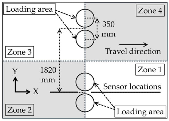
Figure 6.
Loading axle over the pavement surface (not to scale).
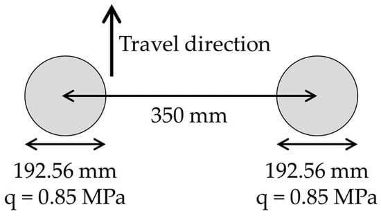
Figure 7.
Static loading configuration at each axle side (not to scale).
6.3. Model Geometry in FEM
The 3D FEM model included only zones 1 and 2 from Figure 6, taking advantage of geometrical symmetry. The model dimensions were designed to extend at least 50 times the static loading radius from the centre of loading in the horizontal direction and 100 times the static loading radius in depth. Infinite elements were applied at the sides and bottom of the model to simulate an infinite medium for the soil layers [55]. The model used 20-node quadratic brick elements, with a mesh size of 25 mm directly under the load and a progressively coarser mesh further away. Dynamic implicit solving method was employed, with a maximum time increment of 0.001 s. The travel distance was set to 1 m along the pavement surface. Figure 8 illustrates the 3D FEM model, with a magnified section showing the mesh in the vicinity of the loading area.
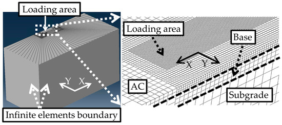
Figure 8.
3D FEM model.
7. Results and Discussion
7.1. Validation of the Correct Implementation of the ODE45 Numerical Solver
Table 5 presents the IRI values calculated using the ODE45 numerical solver for three surface profiles examined in this study, alongside the corresponding IRI values from the LTPP database. As shown, there is a close agreement between the two sets of IRI values, supporting the validity of the ODE45 solver implementation. To illustrate an example of vertical accelerations obtained from the ODE45 solver, Figure 9 shows the results from the analysis of the MN surface profile using Equation (5) and highlights the locations of maximum attenuation and amplification in the tyre load magnitude along the surface profile.

Table 5.
IRI values for the pavement surface profiles.
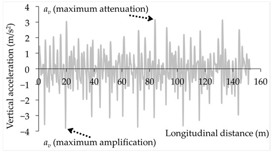
Figure 9.
Vertical accelerations in MN surface profile.
7.2. Validation of FEM Simulations
FEM simulations were validated in two stages. In the first stage, the pavement system was subjected to static analysis, and surface deflections at multiple offset distances from the centre of loading were compared with the corresponding results from the well-established multilayer elastic software CIRCLY [56] and WinJULEA [57]. Figure 10 illustrates this comparison.
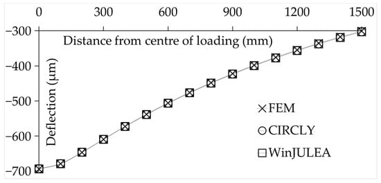
Figure 10.
Comparison of FEM surface deflections with CIRCLY and WinJULEA outputs.
In the second stage, the pavement system was analysed under a moving load using both FEM and the 3D-Move programme. The maximum tensile strain at the bottom of the AC layer and the maximum compressive strain at the top of the subgrade were compared with each other, as shown in Figure 11. It should be noted that to utilise the predefined axle/tyre configurations in 3D-Move, an equivalent single circular loading area with a radius of 136.2 mm was applied on each side of the loading axle during the second stage of validation.
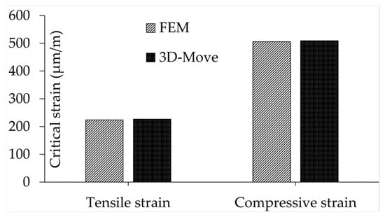
Figure 11.
Comparison of FEM critical strains with 3D-Move outputs.
7.3. Comparison of FEM and Greenwood Engineering TSD Backcalculation Tool
Table 6 presents the backcalculated moduli obtained using the Greenwood Engineering TSD backcalculation tool for various axle load magnitudes, which vary in this study due to the influence of pavement surface roughness. The 10.1-tonne (99 kN) load shown in the table corresponds to the static axle load adopted in this study, without any attenuation or amplification effects. Figure 12 illustrates the backcalculation errors, expressed as the percentage difference between the backcalculated modulus and the FEM modulus for each pavement layer, with the FEM moduli serving as the reference for comparisons.

Table 6.
Backcalculated layers’ moduli for various axle loads.
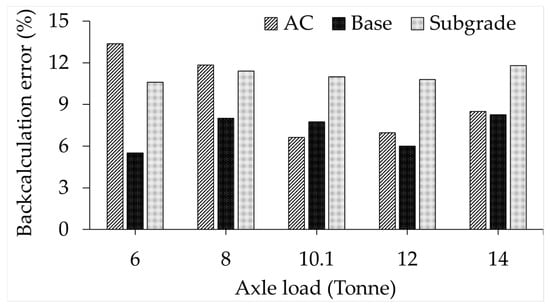
Figure 12.
Backcalculation errors by comparing FEM and TSD backcalculation tool.
As shown in Figure 12, the backcalculation errors between the FEM and the backcalculation tool were always below 13.5% for all pavement layers. This shows that the Greenwood Engineering tool could be reliably used to backcalculate pavement layers’ moduli from TSD deflection slopes throughout the study. To maintain consistency in the comparisons and analyses, the backcalculated moduli corresponding to the static axle load of 10.1 tonnes presented in Table 6 were used as the reference for all subsequent comparisons in this study.
7.4. Effect of Tyre Load Attenuation and Amplification on Backcalculated Moduli
Figure 13 shows an example of deflection slopes obtained from attenuated and amplified loading analyses related to the PA state surface profile. It can be seen that both attenuated and amplified loading conditions have a significant effect on the deflection slopes compared with the case of the TSD’s static axle load. As a result, the influence of these changes in deflection slopes, caused by pavement surface roughness affecting the tyre load magnitude, on the backcalculated moduli of the pavement layers was examined.
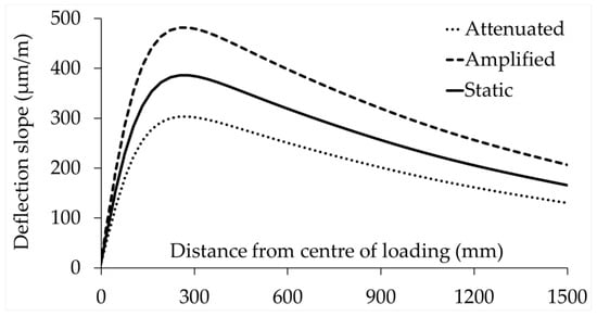
Figure 13.
Deflection slopes at attenuated, amplified, and static tyre load of PA surface profile.
Table 7 presents the backcalculated moduli of pavement layers under the highest attenuation and amplification of tyre load magnitudes caused by pavement surface roughness, as well as under the static tyre load magnitude based on three pavement surface profiles. Figure 14 illustrates the backcalculation errors as percentage differences between the backcalculated moduli of pavement layers under attenuated or amplified load conditions, and those under static load conditions, using the backcalculated moduli under static load cases as the basis for comparisons. As shown, tyre load attenuation and amplification altered the backcalculated moduli of pavement layers by up to 48% and 30%, respectively, in this study.

Table 7.
Backcalculated layers’ moduli in highest attenuation and amplification loading conditions.
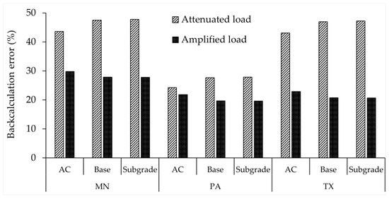
Figure 14.
Backcalculation errors in highest attenuation and amplification loading conditions.
7.5. Effect of Averaging Deflection Slopes on Backcalculated Moduli
At each point set possessing different auxiliary point intervals, deflection slopes were averaged across all points in the set. The backcalculated moduli derived from the averaged deflection slopes were compared with the corresponding backcalculated moduli obtained under the static tyre load, as would occur on a perfectly smooth pavement profile. Figure 15 presents an example of backcalculation errors for the AC layer at the MN surface profile, expressed as the percentage difference between the backcalculated moduli derived from averaged deflection slopes and those obtained using the static tyre load magnitude without averaging the deflection slopes. It should be noted that the backcalculated moduli obtained from the static tyre load magnitude case were used as the basis for comparisons. The numbers above the bars in the graph show the total number of points in each point set that were included in averaging the deflection slopes. The overall trend shown in Figure 15 indicates that reducing the point set interval, which increases the number of auxiliary points in the point set, tends to decrease the backcalculation error.
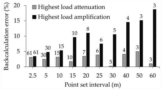
Figure 15.
Backcalculation errors of AC layer by averaging deflection slopes in MN surface profile. (The numbers above the bars show the point count in each point set.)
Predictive equations were developed to correlate the backcalculation error of each pavement layer in each surface profile, under the highest attenuation and amplification of tyre load, with the total number of points in each point set. The mean absolute percentage error (MAPE) was used, based on Equation (9), to evaluate the accuracy of the developed predictive equations. However, the MAPE becomes unreliable when the values under investigation are small [58]. As shown in Figure 15, for example, the backcalculation errors can be less than 5%, thereby reducing the reliability of the MAPE in assessing the accuracy of the predictive equations. Consequently, the backcalculated moduli were first correlated with the number of points in each point set. Since the backcalculated moduli have higher magnitudes than the backcalculation errors, this approach increases the accuracy of the MAPE analysis. The backcalculation errors were then calculated from the backcalculated moduli, enabling the predictive equations to establish a relationship between backcalculation error and the number of points in the point set. As an example of this procedure, Figure 16 presents the backcalculated modulus for the AC layer plotted against the total number of points in the point set for the MN surface profile, considering the loading case with the highest amplification. The results indicate an approximately linear trend on a logarithmic scale. Noting that the backcalculated AC modulus under the static axle loading case, obtained as 2801 MPa and presented in Table 7, was used to calculate the backcalculation error from the backcalculated modulus using Equation (10), the predictive equation for the backcalculated modulus shown in Figure 16 was then used to obtain the backcalculation error prediction using Equation (11).
where i = specified point in the point set, n = number of total points in the point set, = actual backcalculated modulus, and = predicted backcalculated modulus.
where Er(%) = percentage of backcalculation error, E = backcalculated modulus in MPa, and P = the number of points in the point set.
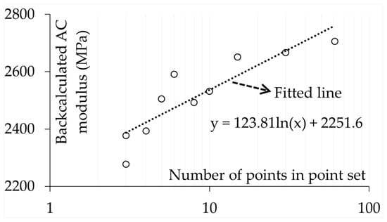
Figure 16.
Backcalculated AC modulus versus number of points in the point set at MN surface profile and highest amplification load case.
It should be noted that the maximum number of points in the point sets occurs when the 2.5 m auxiliary point set intervals are considered. Given the total profile length of 150 m, the maximum number of points in the point sets cannot exceed 61. This total of 61 points includes the point with the highest attenuation and amplification of the tyre load, along with 60 auxiliary points obtained by dividing the profile length of 150 m into 2.5 m intervals. Consequently, the predictive equations correlating backcalculation errors with the number of points in the point set are valid only when the calculated number of points does not exceed 61. Table 8 presents the MAPE values for the regression-based equations used to predict the backcalculated moduli from the number of points in the point set, which were then used to develop equations for predicting backcalculation errors from the number of points in the point set. As can be seen, all MAPE values for the developed predictive equations in Table 8 are below 3.2%, indicating high prediction accuracy based on the criteria presented in Table 9 [59].

Table 8.
Accuracy of backcalculated moduli predictions from number of points in the point set.

Table 9.
Accuracy of forecasting based on MAPE value (data from [59]).
7.6. Effect of Point Set Size on Backcalculation Error
The flowchart shown in Figure 17 explains the overall process used to determine the number of points in a point set required to limit the error in predicting pavement layers’ moduli by averaging deflection slopes. Backcalculation errors of 5% and 10% were considered acceptable tolerance levels in this study. Error tolerances with both positive and negative signs, for example −5% and +5%, were input into the predictive equations correlating backcalculation error with the number of points in the point set, an example of which is shown in Equation (11). This produced two point set numbers denoted by P− and P+, for each error tolerance of 5% and 10% for each pavement layer, corresponding to each condition of attenuation or amplification of tyre load at each surface profile. The smaller of the two point set numbers, referred to as Pmin, was then used as the minimum number of points required in the point set to meet the target error tolerance. Consequently, for each error tolerance of 5% and 10%, a total of 18 values of Pmin were calculated, accounting for variations in surface profiles, loading conditions, and pavement layers. All calculated Pmin values were verified to be below 61, consistent with the maximum number of points in a point set considered in this study, as discussed earlier. The largest value among all Pmin values for each error tolerance was used as the required number of points in the point set, denoted by Ptarget. This ensures the specified backcalculation error tolerance is satisfied across all conditions after averaging deflection slopes. Table 10 presents the calculated Pmin values corresponding to backcalculation error tolerances of 5% and 10%. Based on these results, the minimum number of points required in the point set to achieve a backcalculation error tolerance of 5% is 28, and for 10%, it is 9.
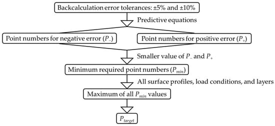
Figure 17.
Flowchart depicting the procedure to calculate required number of points in the point set to limit the backcalculation error.

Table 10.
Required point numbers in the point set for each backcalculation error tolerance.
It should be noted that based on the analyses in this study where deflection slopes were averaged over evaluation points spaced at equal intervals, averaging over 9 points which produced eight distance intervals, corresponds theoretically to a spacing of 150 m divided by 8 or approximately 18.8 m between points. Similarly, averaging over 28 points which produced 27 intervals corresponds to a spacing of 150 m divided by 27 or approximately 5.6 m between points. However, the attenuation or amplification of the tyre load at each evaluation point is highly random, so the exact averaging interval is of lesser importance. Therefore, the number of points used to average the deflection slopes is the primary factor determining the accuracy of the backcalculation.
8. Conclusions
The TSD moving load was simulated in FEM to pass over a three-layer flexible pavement system. The pavement system was assumed to have a rough surface condition, with three different IRI values of 2.77, 3.04, and 3.18 m/km assigned over a 150 m section of the pavement. The purpose of the study was to perform a quantitative analysis using a deterministic approach to evaluate how averaging TSD measurements over different travel-length intervals, which effectively denoises raw TSD signals, can mitigate the negative effect of pavement surface roughness on the backcalculated moduli of pavement layers derived from deflection slopes. This effect arises from changes in deflection slopes caused by the attenuation and amplification of the TSD dynamic load magnitude due to pavement surface roughness.
Using the Greenwood Engineering TSD backcalculation tool, which proved effective for backcalculating from TSD deflection slopes in this study, it was found that the attenuation and amplification of TSD load magnitude caused by pavement surface roughness could lead to up to 48% error in backcalculated moduli of pavement layers. The general trend indicated that averaging deflection slopes over travel-length intervals can reduce backcalculation errors caused by pavement surface roughness. Shorter TSD travel distance intervals, which involve a greater number of points in the averaging process, were found to reduce backcalculation errors more effectively. By correlating backcalculation errors in each pavement layer with the number of points used along the TSD travel direction for averaging deflection slopes, it was found that averaging over 9 equally spaced points could reduce backcalculation errors for all pavement layers to approximately 10%. Increasing the number of points to 28 further reduced the backcalculation error to around 5%.
The results suggest that while averaging deflection slopes is commonly used to eliminate random noise in TSD measurements, it can also mitigate the negative effect of pavement surface roughness on the backcalculated moduli derived from deflection slopes. Therefore, it is important to include a sufficient number of TSD measurement points in the averaging process to effectively minimise the influence of pavement surface roughness on the backcalculation results. Furthermore, averaging the deflection slopes reduces the need to rely on strain gauges for measuring the instantaneous tyre load magnitude affected by pavement surface roughness. This approach helps avoid the uncertainties associated with strain gauges, such as their sensitivity to environmental conditions and the need for regular calibration.
9. Limitations of the Study and Path Towards Future Works
The following limitations exist in this study and warrant consideration, as they not only broaden the understanding of the present findings but also provide a clear pathway for future research:
- -
- The range of IRI values assigned to the pavement surface roughness conditions lay within a narrow range of 2.77 m/km to 3.18 m/km. For this study, rough pavement surface conditions were selected because they have a stronger influence on backcalculation errors. Under these conditions, the negative effects of pavement surface roughness on backcalculated moduli are more pronounced, emphasising the crucial need for the mitigation strategy for backcalculation errors presented in this study. However, assessing a wider range of IRI values would help examine how general the findings are and allow comparisons between different surface roughness conditions when interpreting the results.
- -
- Sources of epistemic or model uncertainty exist in the FEM simulations, and they can be improved in future studies. These include simplifying the viscoelastic behaviour of the AC layer to linear elastic behaviour, ignoring the nonlinear stress-dependent and cross-anisotropic behaviour of the base and subgrade layers, neglecting the effects of moisture change on subgrade stiffness, and using the golden car’s suspension system characteristics to represent the suspension system of the TSD vehicle.
- -
- Given the sources of uncertainty present in the FEM simulations, the deterministic framework used for backcalculation in this study, which produces a unique solution for the backcalculated moduli without considering confidence intervals, appears to be inadequate. In addition to the epistemic uncertainties already discussed, sources of aleatoric or data uncertainty also exist in the TSD backcalculation process. These may include spatial variability in material properties and pavement layers’ thicknesses, TSD measurement noise, and the way IRI averages the surface over distance, which can hide local defects that affect tyre vertical accelerations. Considering all sources of uncertainties, a probabilistic framework for backcalculation that includes uncertainty quantification and provides posterior distributions of the backcalculation outputs, rather than single deterministic values, would be highly valuable. The probabilistic backcalculation approach is a powerful tool for inverse problem solving, as, for example, the Bayesian inference framework has been successfully applied in previous studies [60,61].
- -
- Although only one pavement structure was analysed in this study, the methodology developed to mitigate the negative effect of pavement surface roughness on the backcalculated moduli of pavement layers remains valid and can be applied to different pavement system configurations. However, it is recommended that future studies evaluate a wider range of pavement structures to establish a comprehensive framework for determining the required number of points in a point set to mitigate backcalculation errors to any target error tolerance level.
Author Contributions
Conceptualisation, N.K. and M.S.; methodology, N.K.; validation, N.K.; formal analysis, N.K.; investigation, N.K.; writing—original draft preparation, N.K.; writing—review and editing, M.S. and C.-L.L.; visualisation, N.K.; supervision, M.S. and C.-L.L. All authors have read and agreed to the published version of the manuscript.
Funding
This research received no external funding.
Data Availability Statement
The data presented in this study are available on request from the corresponding author.
Conflicts of Interest
The authors declare no conflicts of interest.
Abbreviations
The following abbreviations are used in this manuscript:
| 2.5D | Two-and-a-half-dimensional |
| 3D | Three-dimensional |
| AC | Asphalt concrete |
| ANN | Artificial neural network |
| CEKF | Constrained extended Kalman filter |
| DLC | Dynamic load coefficient |
| FEM | Finite element method |
| FWD | Falling weight deflectometer |
| GPR | Ground-penetrating radar |
| IRI | International Roughness Index |
| LTPP | Long-Term Pavement Performance |
| MAPE | Mean absolute percentage error |
| MN | Minnesota |
| ODE | Ordinary differential equation |
| PA | Pennsylvania |
| SAFEM | Semi-analytical finite element method |
| SDR | Standard Data Release |
| SHRP | Strategic Highway Research Program |
| TSD | Traffic speed deflectometer |
| TX | Texas |
References
- Douglas, A.S.; Lee, H.; Beckemeyer, C.A. Development of the Rolling Wheel Deflectometer (RWD); Report No. FHWA-DTFH-61-14-H00019; Federal Highway Administration, U.S. Department of Transportation: Washington, DC, USA, 2020. [Google Scholar]
- Rada, G.R.; Nazarian, S.; Visintine, B.A.; Siddharthan, R.; Thyagarajan, S. Pavement Structural Evaluation at the Network Level: Final Report; Report No. FHWA-HRT-15–074; Federal Highway Administration, U.S. Department of Transportation: Washington, DC, USA, 2016. [Google Scholar]
- Krarup, J.; Rasmussen, S.; Aagaard, L.; Hjorth, P.G. Output from the Greenwood Traffic Speed Deflectometer. In Proceedings of the 22nd ARRB Conference—Research into Practice, Canberra, Australia, 29 October–2 November 2006. [Google Scholar]
- Canestrari, F.; Ingrassia, L.P.; Spinelli, P.; Graziani, A. A New Methodology to Assess the Remaining Service Life of Motorway Pavements at the Network Level from Traffic Speed Deflectometer Measurements. Int. J. Pavement Eng. 2023, 24, 2128349. [Google Scholar] [CrossRef]
- Shen, K.; Wang, H. Prediction of Critical Strains of Flexible Pavement from Traffic Speed Deflectometer Measurements. Constr. Build. Mater. 2024, 411, 134770. [Google Scholar] [CrossRef]
- Zhang, M.; Gong, H.; Jia, X.; Jiang, X.; Feng, N.; Huang, B. Determining Pavement Structural Number with Traffic Speed Deflectometer Measurements. Transp. Geotech. 2022, 35, 100774. [Google Scholar] [CrossRef]
- Nielsen, C.P.; Nahoujy, M.R.; Jansen, D. Measuring Joint Movement on Rigid Pavements using the Traffic Speed Deflectometer. J. Transp. Eng. Part B Pavements 2023, 149, 04023002. [Google Scholar] [CrossRef]
- Nasimifar, M.; Thyagarajan, S.; Sivaneswaran, N. Backcalculation of Flexible Pavement Layer Moduli from Traffic Speed Deflectometer Data. Transp. Res. Rec. 2017, 2641, 66–74. [Google Scholar] [CrossRef]
- Nielsen, C.P. Visco-elastic Back-calculation of Traffic Speed Deflectometer Measurements. Transp. Res. Rec. 2019, 2673, 439–448. [Google Scholar] [CrossRef]
- Marcondes, J.A.; Snyder, M.B.; Singh, S.P. Predicting Vertical Acceleration in Vehicles through Road Roughness. J. Transp. Eng. 1992, 118, 33–49. [Google Scholar] [CrossRef]
- Misaghi, S.; Tirado, C.; Nazarian, S.; Carrasco, C. Impact of Pavement Roughness and Suspension Systems on Vehicle Dynamic Loads on Flexible Pavements. Transp. Eng. 2021, 3, 100045. [Google Scholar] [CrossRef]
- Siddharthan, R.V.; Yao, J.; Sebaaly, P.E. Pavement Strain from Moving Dynamic 3D Load Distribution. J. Transp. Eng. 1998, 124, 557–566. [Google Scholar] [CrossRef]
- Zihan, Z.U.; Elseifi, M.A.; Icenogle, P.; Gaspard, K.; Zhang, Z. Mechanistic-based Approach to Utilize Traffic Speed Deflectometer Measurements in Backcalculation Analysis. Transp. Res. Rec. 2020, 2674, 208–222. [Google Scholar] [CrossRef]
- Wu, C.; Wang, H.; Zhao, J.; Jiang, X.; Qiu, Y. Asphalt Pavement Modulus Backcalculation using Surface Deflections under Moving Loads. Comput.-Aided Civ. Infrastruct. Eng. 2020, 35, 1246–1260. [Google Scholar] [CrossRef]
- McCormack, R. TRUCKSIM—A Log Truck Performance Simulator. J. For. Eng. 1990, 2, 31–37. [Google Scholar] [CrossRef]
- Shen, K.; Wang, H. Impact of Dynamic Loading on Pavement Deflection Measurements from Traffic Speed Deflectometer. Measurement 2023, 217, 113086. [Google Scholar] [CrossRef]
- Dai, J.; Adhikari, S.; Wen, M. Uncertainty Quantification and Propagation in Atomistic Machine Learning. Rev. Chem. Eng. 2025, 41, 333–357. [Google Scholar] [CrossRef]
- Flintsch, G.W.; Ferne, B.; Diefenderfer, B.; Katicha, S.; Bryce, J.; Nell, S. Evaluation of Traffic-Speed Deflectometers. Transp. Res. Rec. 2012, 2304, 37–46. [Google Scholar] [CrossRef]
- Katicha, S.W.; Flintsch, G.W.; Ferne, B. Optimal Averaging and Localized Weak Spot Identification of Traffic Speed Deflectometer Measurements. Transp. Res. Rec. 2013, 2367, 43–52. [Google Scholar] [CrossRef]
- Katicha, S.W.; Flintsch, G.; Bryce, J.; Ferne, B. Wavelet Denoising of TSD Deflection Slope Measurements for Improved Pavement Structural Evaluation. Comput.-Aided Civ. Infrastruct. Eng. 2014, 29, 399–415. [Google Scholar] [CrossRef]
- Katicha, S.W.; Bryce, J.; Flintsch, G.; Ferne, B. Estimating “True” Variability of Traffic Speed Deflectometer Deflection Slope Measurements. J. Transp. Eng. 2015, 141, 04014071. [Google Scholar] [CrossRef]
- Wu, C.; Duan, Y.; Wang, H. Signal Denoising of Traffic Speed Deflectometer Measurement Based on Partial Swarm Optimization–Variational Mode Decomposition Method. Sensors 2024, 24, 3708. [Google Scholar] [CrossRef]
- Rada, G.; Nazarian, S.; Tirado, C.; Beizaei, M.; Flintsch, G.; Katicha, S. Verification of Traffic Speed Deflection Devices’ (TSDDs) Measurements: Final Report; Project No. 10-105; NCHRP Transportation Research Board of the National Academies of Sciences, Engineering, and Medicine: Washington, DC, USA, 2023. [Google Scholar]
- Zhang, M.; Fu, G.; Ma, Y.; Xiao, R.; Huang, B. Speed and Temperature Superposition on Traffic Speed Deflectometer Measurements. Transp. Geotech. 2023, 40, 100990. [Google Scholar] [CrossRef]
- Hoffmann, K. An Introduction to Measurements Using Strain Gages; Hottinger Baldwin Messtechnik GmbH: Darmstadt, Germany, 1989. [Google Scholar]
- Florin, A.; Ioan-Cozmin, M.-R.; Liliana, P. Passive Suspension Modeling Using MATLAB, Quarter Car Model, Input Signal Step Type. In Proceedings of the 17th International TEHNOMUS Conference (New Technologies and Products in Machine Manufacturing Technologies), Suceava, Romania, 17–18 May 2013; pp. 258–263. [Google Scholar]
- Sandage, R.N.; Patil, P.M.; Patil, S. Simulation Analysis of 2DOF Quarter Car Semi-Active Suspension System to Improve Ride comfort—A review. Int. J. Appl. Innov. Eng. Manag. (IJAIEM) 2013, 2, 339–345. [Google Scholar]
- Cruz, O.G.D.; Mendoza, C.A.; Lopez, K.D. International Roughness Index as Road Performance Indicator: A Literature Review. In Proceedings of the International Conference on Contemporary and Sustainable Infrastructure (ICCSI), Bangalore, India, 21–22 May 2021. [Google Scholar] [CrossRef]
- Pawar, P.R.; Mathew, A.T.; Saraf, M. IRI (International Roughness Index): An Indicator of Vehicle Response. In Materials Today, Proceedings of the International Conference on Materials, Manufacturing and Modelling (ICMMM), Vellore, India, 9–12 March 2017; Elsevier Ltd.: Amsterdam, The Netherlands, 2018; Volume 5, pp. 11738–11750. [Google Scholar] [CrossRef]
- Arhin, S.A.; Noel, E.C. Predicting Pavement Condition Index Using International Roughness Index in Washington DC: Final Report; Report No. DDOT-RDT-14-03; Department of Transportation: Washington, DC, USA, 2014. [Google Scholar]
- Múčka, P. International Roughness Index Specifications Around the World. Road Mater. Pavement Des. 2017, 18, 929–965. [Google Scholar] [CrossRef]
- Di Mascio, P.; Loprencipe, G.; Moretti, L.; Puzzo, L.; Zoccali, P. Bridge Expansion Joint in Road Transition Curve: Effects Assessment on Heavy Vehicles. Appl. Sci. 2017, 7, 599. [Google Scholar] [CrossRef]
- Sayers, M.W.; Karamihas, S.M. The Little Book of Profiling: Basic Information About Measuring and Interpreting Road Profile; Transportation Research Institute, University of Michigan: Ann Arbor, MI, USA, 1998. [Google Scholar]
- Greenwood Engineering. TSD Viscoelastic back Calculation. Available online: https://vbc.greenwood.dk/ (accessed on 6 October 2023).
- Maser, K.; Schmalzer, P.; Shaw, W.; Carmichael, A. Integration of Traffic Speed Deflectometer and Ground-Penetrating Radar for Network-Level Roadway Structure Evaluation. Transp. Res. Rec. 2017, 2639, 55–63. [Google Scholar] [CrossRef]
- Federal Highway Administration. LTPP Standard Data Release, Long-Term Pavement Performance Program, SDR 37. Available online: https://infopave.fhwa.dot.gov/Data/StandardDataRelease (accessed on 11 December 2023).
- Bilodeau, J.-P.; Gagnon, L.; Doré, G. Assessment of the Relationship Between the International Roughness Index and Dynamic Loading of Heavy Vehicles. Int. J. Pavement Eng. 2017, 18, 693–701. [Google Scholar] [CrossRef]
- MATLAB, version 9.13.0; The MathWorks Inc.: Natick, MA, USA, 2022.
- ABAQUS; Dassault Systèmes Simulia Corp.: Johnston, RI, USA, 2022.
- Liu, X.; Al-qadi, I. Integrated Vehicle–Tire–Pavement Approach for Determining Pavement Structure–Induced Rolling Resistance under Dynamic Loading. Transp. Res. Rec. 2022, 2676, 398–409. [Google Scholar] [CrossRef]
- Wang, Z.Z.; Sun, Z.; Hakim, B.; Indraratna, B.; Al-Tabbaa, A. Probabilistic Simulation of TSD-based Pavement Deflections for Bayesian Updating of Material Parameters. Transp. Geotech. 2025, 55, 101715. [Google Scholar] [CrossRef]
- Nasimifar, M.; Kamalizadeh, R.; Heidary, B. The Available Approaches for using Traffic Speed Deflectometer Data at Network Level Pavement Management System. Measurement 2022, 202, 111901. [Google Scholar] [CrossRef]
- Mejłun, Ł.; Judycki, J.; Dołżycki, B. Comparison of Elastic and Viscoelastic Analysis of Asphalt Pavement at High Temperature. Procedia Eng. 2017, 172, 746–753. [Google Scholar] [CrossRef]
- Moffatt, M. Guide to Pavement Technology Part 2: Pavement Structural Design; Austroads Ltd.: Sydney, Australia, 2017. [Google Scholar]
- NOAA National Centers for Environmental Information. Climate at a Glance: Statewide Time Series. Available online: https://www.ncei.noaa.gov/access/monitoring/climate-at-a-glance/statewide/time-series (accessed on 2 December 2025).
- Brown, S.F.; Pappin, J. Analysis of Pavements with Granular Bases. Transp. Res. Rec. 1981, 810, 17–23. [Google Scholar]
- Uzan, J. Characterization of Granular Material. Transp. Res. Rec. 1985, 1022, 52–59. [Google Scholar]
- Al-Qadi, I.L.; Wang, H.; Tutumluer, E. Dynamic Analysis of Thin Asphalt Pavements by using Cross-Anisotropic Stress-Dependent Properties for Granular Layer. Transp. Res. Rec. 2010, 2154, 156–163. [Google Scholar] [CrossRef]
- Tarefder, R.A.; Ahmed, M.U.; Rahman, A. Effects of Cross-Anisotropy and Stress-Dependency of Pavement Layers on Pavement Responses under Dynamic Truck Loading. J. Rock Mech. Geotech. Eng. 2016, 8, 366–377. [Google Scholar] [CrossRef]
- Kazemi, N.; Saleh, M.; Lee, C.-L. Effect of the Stress Dependency and Anisotropy of Unbound Granular Base and Subgrade Materials on TSD Deflection Slopes. In Proceedings of the International Conference on Transportation and Development (ICTD), Atlanta, GA, USA, 15–18 June 2024; pp. 327–337. [Google Scholar] [CrossRef]
- Kazemi, N.; Saleh, M.; Lee, C.-L. Effect of Nonlinear Stress-Dependency and Cross-Anisotropy on the Backcalculation Outputs from the TSD Deflection Slopes and the Effect on Estimated Pavement Performance. Int. J. Pavement Eng. 2024, 25, 2417967. [Google Scholar] [CrossRef]
- Hamidi, A.; Hoff, I.; Mork, H. A Sensitivity Analysis on the Simulated Measurements of Traffic Speed Deflection Devices. Int. J. Pavement Eng. 2024, 25, 2447461. [Google Scholar] [CrossRef]
- ABAQUS 2016 User Subroutines Reference Guide; Dassault Systèmes Simulia Corp.: Providence, RI, USA, 2015.
- Fortran Compiler, Intel Corporation: Santa Clara, CA, USA, 2023.
- ABAQUS Theory Manual: Version 6.11; Dassault Systèmes Simulia Corp.: Providence, RI, USA, 2011.
- Wardle, L. CIRCLY and Mechanistic Pavement Design: The Past, Present and Towards the Future; Mincad Systems: Richmond, Australia, 2010. [Google Scholar]
- Uzan, J. JULEA (Jacob Uzan Layered Elastic Analysis); Technion University: Haifa, Israel, 1976. [Google Scholar]
- Kim, S.; Kim, H. A New Metric of Absolute Percentage Error for Intermittent Demand Forecasts. Int. J. Forecast. 2016, 32, 669–679. [Google Scholar] [CrossRef]
- Lewis, C.D. Industrial and Business Forecasting Methods: A Practical Guide to Exponential Smoothing and Curve Fitting; Butterworth Scientific: London, UK, 1982; ISBN 978-0408005593. [Google Scholar]
- Wang, H.; Zhou, W.; Wang, H.; Li, G. A DeepONets-based Resolution Independent ABC Inverse Method for Determining Material Parameters of HAZ. Eng. Fract. Mech. 2025, 315, 110843. [Google Scholar] [CrossRef]
- Jiang, X.; Wang, X.; Wen, Z.; Wang, H. Resolution-Independent Generative Models based on Operator Learning for Physics-Constrained Bayesian Inverse Problems. Comput. Methods Appl. Mech. Eng. 2024, 420, 116690. [Google Scholar] [CrossRef]
Disclaimer/Publisher’s Note: The statements, opinions and data contained in all publications are solely those of the individual author(s) and contributor(s) and not of MDPI and/or the editor(s). MDPI and/or the editor(s) disclaim responsibility for any injury to people or property resulting from any ideas, methods, instructions or products referred to in the content. |
© 2025 by the authors. Licensee MDPI, Basel, Switzerland. This article is an open access article distributed under the terms and conditions of the Creative Commons Attribution (CC BY) license (https://creativecommons.org/licenses/by/4.0/).