Article

Temperature and Speed Corrections for TSD-Measured Deflection Slopes Using 3D Finite Element Simulations

Department of Civil and Environmental Engineering, University of Canterbury, Christchurch 8140, New Zealand
*
Author to whom correspondence should be addressed.
Infrastructures 2025, 10(12), 351; https://doi.org/10.3390/infrastructures10120351
Submission received: 28 October 2025 / Revised: 12 December 2025 / Accepted: 15 December 2025 / Published: 16 December 2025

Abstract

Traffic Speed Deflectometer (TSD) measures deflection velocities, normalised by travel speed to obtain deflection slopes. Pavement temperature and travel speed can significantly affect deflection slopes. Therefore, correcting deflection slopes for temperature and speed effects is essential. This study employs three-dimensional (3D) finite element simulations of a three-layer flexible pavement system subjected to moving load at travel speeds from 40 km/h to 80 km/h, while varying the Asphalt Concrete (AC) layers’ thickness from 100 mm to 300 mm and the temperature from 5 °C to 45 °C. The results showed that deflection slopes at 100 mm offset distance could be corrected for the effects of temperature and speed using a correction factor comprising the sum of a parabolic function of temperature and a linear function of speed. At 600 mm and 1500 mm offset distances, simpler correction factors could be established using the sum of linear functions of temperature and speed. The Mean Absolute Percentage Error (MAPE) for all predictions was below 3%, indicating high accuracy. Accurate regression-based equations were also proposed to incorporate AC thickness in predicting the correction factors. The results highlight the potential to correct deflection slopes to a reference temperature and speed by evaluating a range of pavement systems.

1. Introduction

Several parameters influence the deformation and performance of the Asphalt Concrete (AC) layer, one of which is temperature. As the temperature increases, the stiffness of the AC layer decreases [1]. Therefore, it is essential to adjust pavement surface deflections or their analysis for temperature effects to ensure a reasonable interpretation [2]. The viscoelastic characteristics of the AC layer in flexible pavement systems also mean that deflections are affected by travel speed as well as temperature [3], so adjustment for speed effects is equally necessary. The correction of Falling Weight Deflectometer (FWD) deflections for temperature has been studied, and the American Association of State Highway and Transportation Officials (AASHTO) [4] developed charts to adjust FWD deflections based on the AC layer’s thickness and temperature. However, temperature correction for measurements obtained from Traffic Speed Deflection Devices (TSDDs), such as the Traffic Speed Deflectometer (TSD), is still under development. The TSD operates at traffic speed, carrying a set of laser sensors enclosed in a steel container mounted on a single rear-axle trailer. These sensors are positioned both ahead of and behind the loading axle. Using the Doppler effect, the sensors measure deflection velocities, which are then normalised by the travel speed to produce deflection slopes as outputs [5].
Rada et al. [6] proposed a temperature correction factor based on the pavement temperature at the time of TSDD measurement and a reference temperature of 21.11 °C. This factor was used to adjust the dynamic modulus of the AC layer for use in correlation equations with maximum fatigue strains calculated from deflection-based parameters. Shrestha et al. [7] applied the same correction factor from Rada et al. [6] to modify the AC layer’s dynamic modulus. By determining the corrected fatigue strain at the reference temperature, they then used correlation equations to derive a temperature-corrected Surface Curvature Index (SCI300) parameter. Nasimifar et al. [8] generated a synthetic database of SCI300 values using the 3D-Move programme [9] and applied the functional forms developed by Lukanen et al. [2] to propose a temperature adjustment factor that accounts for the reference temperature, the AC layer’s thickness, and the latitude of the measurement location to correct the SCI300 parameter. Zhang et al. [3] introduced the effective temperature correction method that simultaneously accounts for both speed and temperature effects on TSD deflections simulated using the 3D-Move programme. Their study also revealed that TSD deflections are influenced much more by pavement temperature than by TSD travel speed. As shown in previous studies, all correction approaches accounting for the effects of temperature and speed were proposed by considering deflections or deflection-based parameters. However, TSD does not directly measure pavement surface deflections. Instead, algorithms are used to convert TSD deflection slopes into deflection values and the inaccuracies of these algorithms have been discussed in the literature [10]. In a recent study, a synthetic database of TSD deflections and deflection slopes was developed using the Semi-Analytical Finite Element Method (SAFEM). Simple linear regression equations with R2 values between 85% and 90% were proposed to estimate the temperature correction factor (TCF) for deflection slopes, based on the temperature at the mid-depth of the AC layer and the TSD travel speed. The reference temperature and speed were set at 22 °C and 72 km/h, respectively. To improve the accuracy of TCF predictions, the machine learning approach of developing an Artificial Neural Network (ANN) was also adopted. Based on an evaluation of activation functions, including none, Rectified Linear Unit (ReLU), sigmoid, and hyperbolic tangent, and after testing layer sizes from 2 to 10, a network structure with a layer size of 9 and the sigmoid activation function was selected for developing the ANN. Bayesian optimisation was employed to minimise the target function, defined as the Mean Absolute Error (MAE), during ANN development. The dataset was split into an 80% training subset to establish the ANN and a 20% subset for testing the model [11].
Even though ANN models have been developed to directly correct deflection slopes by accounting for temperature and speed effects, such ANN models are not readily accessible to practitioners and are less practical than simple equations that can be used to estimate correction factors. Some attempts have also been made to develop simple linear regression equations to estimate correction factors for deflection slopes directly. However, developing accurate regression equations requires an understanding of how the correction factors vary with pavement structural parameters, pavement temperature, and TSD travel speed, and this has not been examined in previous studies. Consequently, performing a systematic sensitivity analysis of the factors affecting correction factors for deflection slopes provides a foundation for developing accurate and practically usable equations to correct deflection slopes. Finite Element Method (FEM) simulation of pavement systems has proven effective in TSD-related studies, such as backcalculation of flexible pavement layers’ moduli from TSD measurements [12], investigating TSD measurements in inverted asphalt pavements [13], calculating surface deflections from deflection slopes [14], and predicting speed and temperature correction factors for deflection slopes in flexible pavements using ANNs [11]. Building on the demonstrated effectiveness of FEM in previous TSD-related studies, FEM simulation of flexible pavement systems can also be utilised to perform a sensitivity analysis of the factors influencing correction factors for deflection slopes.

2. Objective and Scope

The main objective of this study is to perform a systematic sensitivity analysis using FEM simulations to evaluate the effects of AC temperature, AC thickness, and TSD travel speed on correction factors for deflection slopes. Understanding the correlations between correction factors and the aforementioned parameters can facilitate the development of accurate and practically applicable equations to predict correction factors.

3. Materials and Methods

In this study, the movement of the rear axle of a TSD trailer over three-layer flexible pavement systems was modelled using three-dimensional (3D) Finite Element Analysis (FEA) in ABAQUS software (version 6.22-1) [15]. Deflection slopes were obtained between the dual wheels on one side of the loading axle where the Doppler equipment is installed. The deflection slopes were captured at offset distances of 100, 200, 300, 600, 900, and 1500 mm from the centre of loading, corresponding to the typical positions of Doppler laser sensors mounted on TSDs in the United States [16]. Further details of the FEM simulations are provided in the subsequent sections.

3.1. Material Properties in FEM

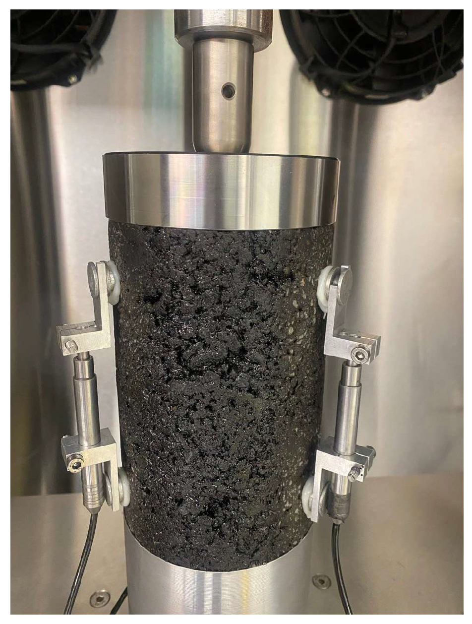
The AC layer was modelled in the FEM using the viscoelastic properties of AC14 mixtures containing Performance Grade (PG) 64-16 binder, sourced from a local contractor in Christchurch, New Zealand. The AC mixtures were prepared using an optimum binder content of 5.6% and compacted with a gyratory compactor applying a ram pressure of 600 kPa and an external gyration angle of 1.25°. Dynamic moduli of four replicates of the AC mixture were measured at different temperatures and loading frequencies in accordance with AASHTO TP 62-07 [17]. The dynamic moduli were then shifted to any reference temperature using the Williams–Landel–Ferry (WLF) shifting function [18] to construct the AC master curve at the target temperature. Equation (1) presents the WLF shifting function. The procedure for fitting the sigmoidal function to the AC master curve, converting it to Prony series, and obtaining the dimensionless shear relaxation modulus for use as ABAQUS-compatible input can be found in other studies [1,19,20,21]. Figure 1 shows the dynamic modulus test apparatus.
Figure 1. Dynamic modulus test setup.
Infrastructures 10 00351 g001
log a T = c 1 × ( T T s ) c 2 + T T s
a T = shift factor;
T = target temperature;
T s = reference temperature;
c 1 & c 2 = material constants.
As an example of the AC material properties used in the FEM simulations, Figure 2 shows the master curve of the AC mixture at 29 °C, while Table 1 lists the corresponding ABAQUS input parameters for the viscoelastic AC layer. The goodness of fit of the Prony series parameters at each reference temperature with respect to the measured dynamic moduli data was evaluated using the Mean Absolute Percentage Error (MAPE), as defined in Equation (2) [22]. Table 2 presents the MAPE for each set of Prony series data fitted to the shifted dynamic moduli at each reference temperature to construct the master curve, along with the WLF shifting function constants for the corresponding temperatures. According to the interpretation of regression accuracy based on MAPE values shown in Table 3 [23], all MAPE values in Table 2 are below 3.5%, indicating a high fitting accuracy for all Prony series.
M A P E = 1 N t = 1 n A t F t A t
t = specified data point;
N = number of data points;
A t = actual value at data point t;
F t = predicted value at data point t.
It should be noted that, in practice, the temperature within the AC layer is not constant and varies with depth. This temperature gradient significantly influences the stress state, particularly in thicker AC layers [24]. However, because temperature changes depend on the time of day and season, considering the exact temperature gradient would introduce considerable uncertainty. Consequently, for pavement structural evaluation, it is common to assign a representative temperature to the entire AC layer, referred to as the effective temperature [25]. Previous studies have suggested different approaches for defining the effective temperature. Although using the temperature at a fixed depth as the effective temperature has previously been recommended [4], other studies have proposed that the effective temperature should depend on the AC layer’s thickness. For instance, Inge and Kim [26] suggested taking the effective temperature at the mid-depth of the AC layer, while Walia et al. [25] recommended using a depth between 30% and 45% of the AC thickness. Based on this discussion, an effective temperature was assumed for the entire AC layer in this study and used in the analyses.
The base and subgrade layers were modelled as linear elastic in the simulations. Although it has been demonstrated that unbound granular materials and fine-grained soils exhibit nonlinear stress-dependent and cross-anisotropic behaviour [27,28,29,30], these characteristics were not considered in this study. However, their effects on TSD deflection slopes and backcalculation results have been investigated in other studies [31,32]. While the Rayleigh damping model is available in ABAQUS for representing material damping [21], it constructs the damping ratio curve using only two frequencies and has several limitations. These include its inability to accurately represent damping across an arbitrary number of modes and its poor performance in achieving a uniform damping ratio [33]. Despite these drawbacks, it remains widely used due to its mathematical simplicity and computational efficiency [34]. Therefore, to avoid introducing unrealistic material damping, the Rayleigh damping model was not applied. Instead, the damping matrix in the FEM simulations was derived solely from the viscoelastic behaviour of the AC layer. Table 4 presents the material properties and layer thicknesses of the pavement systems used in this study.

3.2. Loading Configuration in FEM

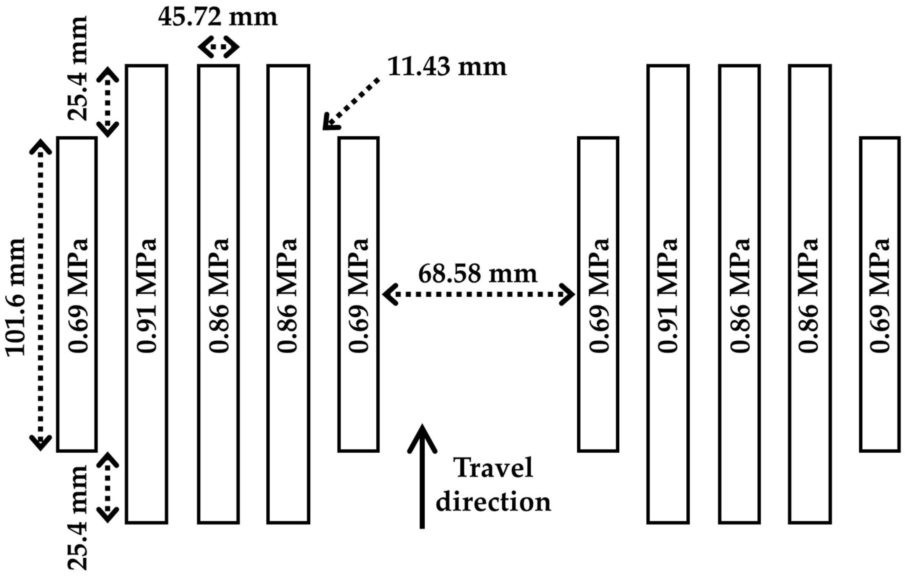
Nasimifar et al. [35] used TSD tyre footprints with non-uniform contact pressure distribution over the tyre grooves at the MnROAD trials and incorporated this loading configuration in their TSD simulations conducted with the 3D-Move programme. This configuration was based on a report from South Africa, where pressure measurement sensors were used to determine the non-uniform contact pressure distribution across the TSD tyres’ loading area [36]. Figure 3 illustrates the tyre footprint loading configuration, showing the non-uniform contact pressure distribution across the loading area on each side of the loading axle. As part of their study, the TSD loading configuration for each tyre shown in Figure 3 was converted into an equivalent circular loading with uniform contact pressure distribution over the contact area, while maintaining the total load of 24.75 kN applied to each tyre and causing only a negligible change in the contact area of around 2%. Figure 4 presents this equivalent dual circular loading configuration on each side of the loading axle, which was adopted to simulate the rear axle of the TSD trailer in this study.
Although some TSD devices intentionally apply more weight to the side containing Doppler equipment to increase deflections under the load [37], an equal axle load distribution was assumed in this study. However, the effects of tyre footprint loading configuration with non-uniform contact pressure distribution and unequal axle load spread on TSD deflection slopes, and the backcalculated moduli derived from deflection slopes have been investigated in other studies by the authors. It should be noted that the TSD travel speeds considered in the simulations were 40, 50, 60, 70, and 80 km/h. DLOAD subroutines [38] were developed using Fortran code [39] to define the movement of the loading configuration across the pavement systems for each travel speed.

3.3. Model Geometry in FEM

Due to the symmetry of the loading axle between the two sides, a 3D half-pavement model was developed and used in this study to simulate the movement of the TSD axle over a 1 m travel distance. The model dimensions were set to extend at least 50 times the loading radius (4953 mm) in the horizontal direction and 100 times the loading radius (9906 mm) in depth. Infinite elements were applied at the sides and bottom of the model to represent the infinite extent of the pavement layers [40]. The 20-node quadratic brick elements were used in the simulations, with an element size of 25 mm near the centre of loading and a progressively coarser mesh at greater distances. A dynamic implicit solving method was used for the analyses, with a maximum time increment of 0.001 s. Figure 5 shows an overview of the 3D FEM model, including a magnified section highlighting the mesh configuration near the loading area.

4. Results and Discussion

4.1. Theoretical Validation of FEM Simulations

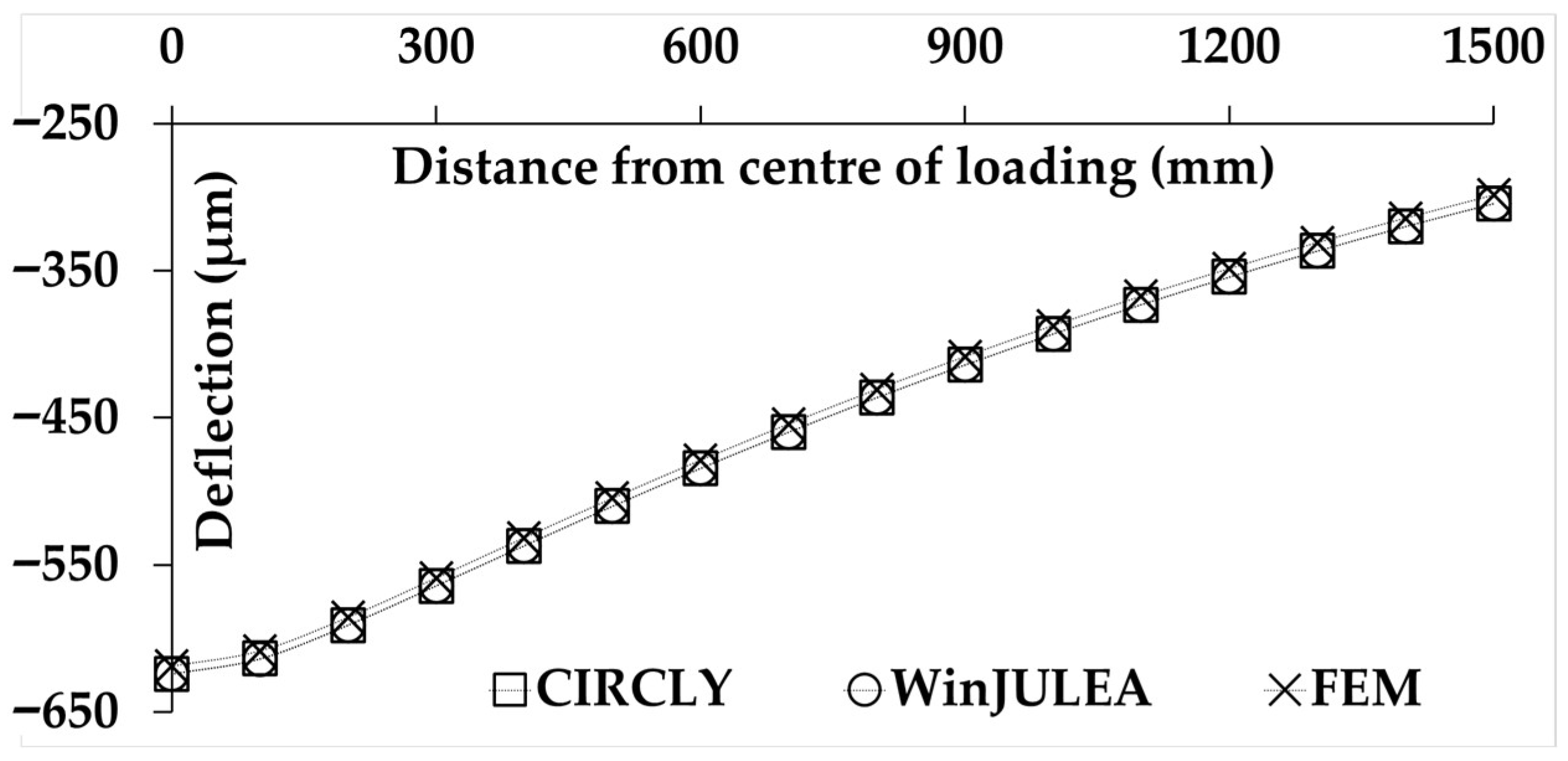
Finite element simulations were theoretically validated in two stages. In the first stage, a pavement system with a 200 mm AC layer and linear elastic material properties for all layers underwent static analysis in FEM. Vertical surface deflections between the dual wheels were obtained at multiple offset distances from the centre of loading and compared with the corresponding results from the multilayer elastic analysis software CIRCLY 7.0 [41] and WinJULEA 1.0 [42]. To reflect the linear elastic behaviour of the AC layer at this stage, an elastic modulus of 3000 MPa was used. Figure 6 presents the comparison of vertical surface deflections.
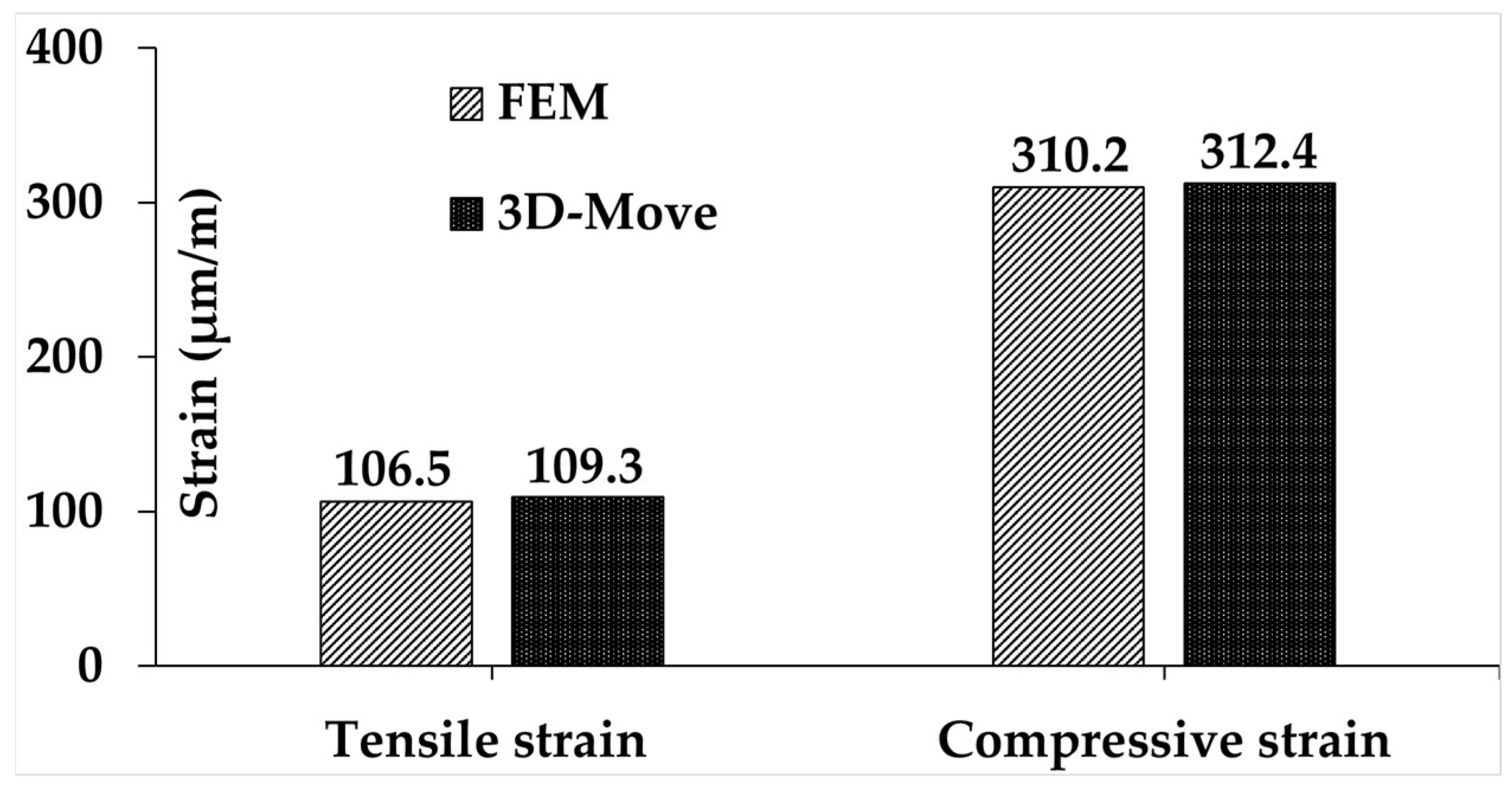
In the second stage of theoretical validation, the pavement system was analysed in FEM using a viscoelastic AC layer with a thickness of 200 mm at a temperature of 21 °C. The maximum tensile strain at the bottom of the AC layer and the maximum compressive strain at the top of the subgrade were obtained and compared with the corresponding results from the 3D-Move programme. To account for the predefined axle/tyre loading configuration in 3D-Move, an equivalent single circular loading area with a radius of 140 mm was applied to each side of the loading axle. A travel speed of 60 km/h was used at this stage of validation. Figure 7 shows the comparison of the critical tensile and compressive strains.
Consequently, by comparing the pavement responses obtained from FEM with the corresponding outputs of well-known software, a close match was observed, thereby providing theoretical validation of the FEM simulations.

4.2. Field Validation of FEM Simulations Based on MnROAD Measurements

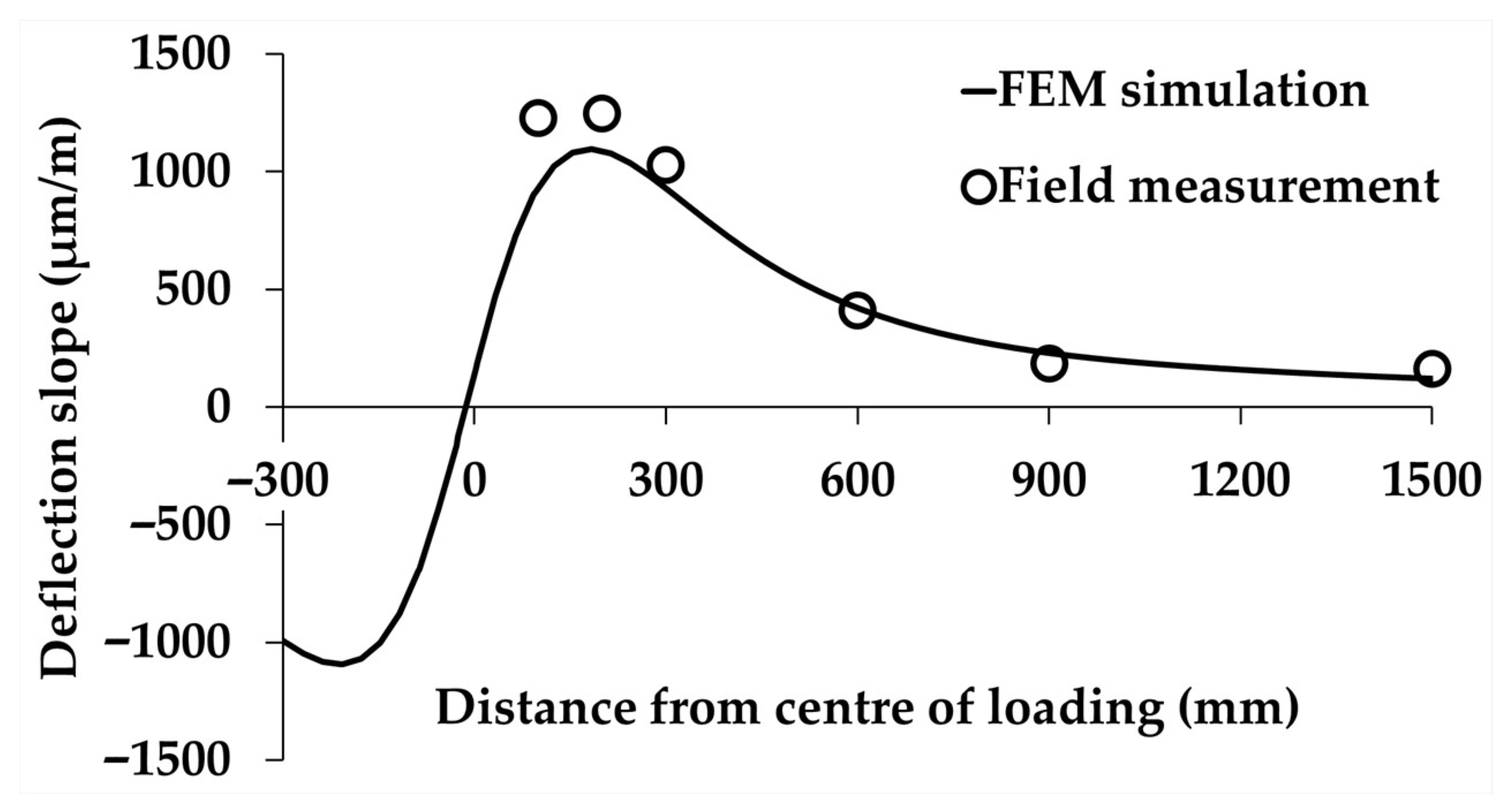
Deflection slopes obtained from TSD field investigations at Cell 19 of the MnROAD facility were used to compare the FEM-generated deflection slopes with field measurements. Details of the material properties and layer thicknesses for the pavement section in Cell 19 are available elsewhere [6]. Figure 8 presents the comparison between FEM and field-measured deflection slopes, showing a close match and thereby validating the FEM simulations against field data.

4.3. Temperature Correction of Deflection Slopes

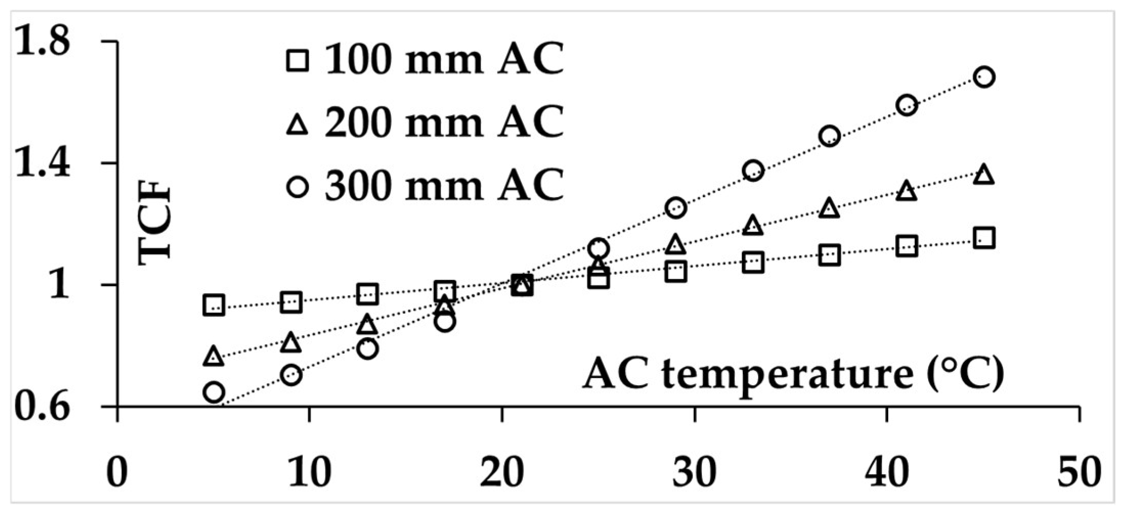
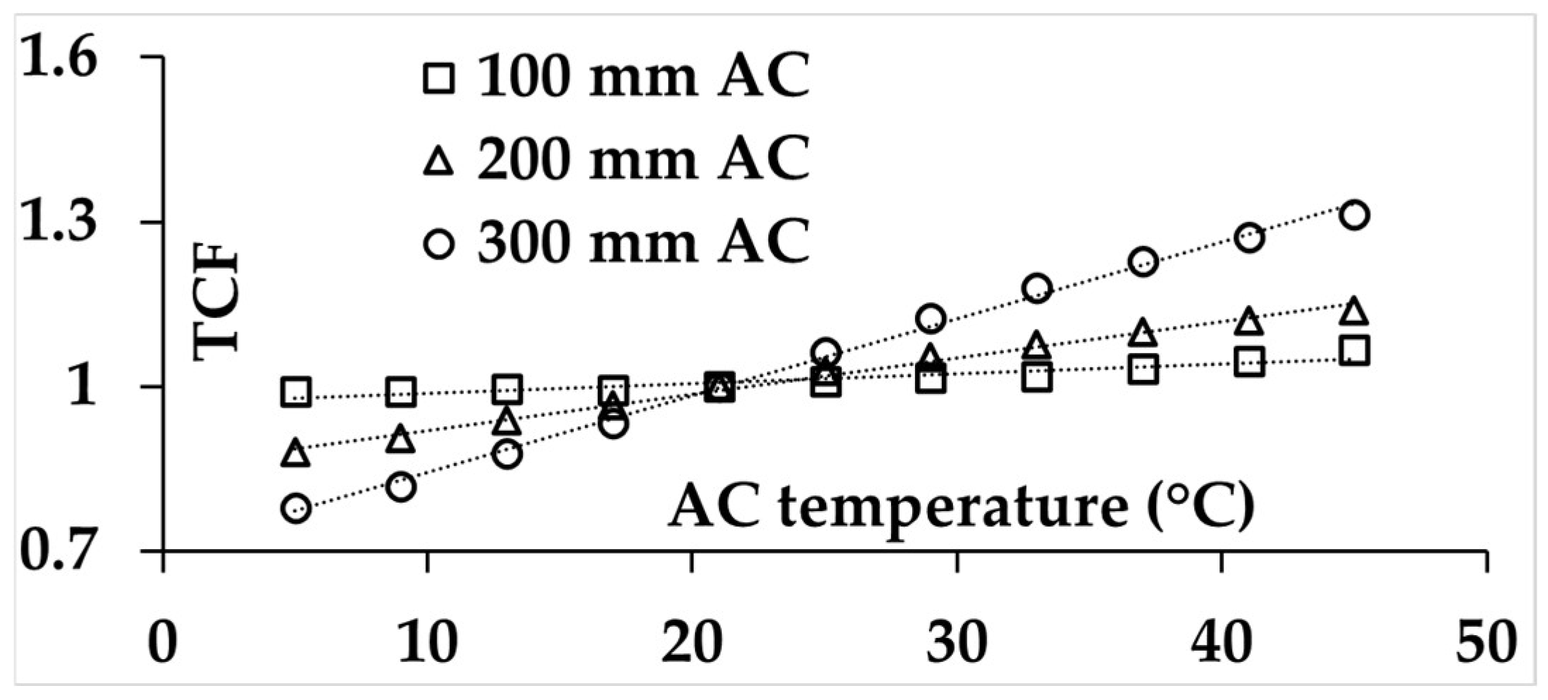
At this stage of the study, deflection slopes obtained at various AC temperatures were corrected to an intermediate AC temperature of 21 °C, which was selected as the reference temperature. Three Doppler laser sensor locations were considered for the analysis, one located near the centre of loading at 100 mm offset distance, one at mid-range offset distance of 600 mm, and one at the furthest offset distance of 1500 mm. The effect of TSD travel speed was not considered at this stage. Instead, a constant speed of 60 km/h was assumed, which represents the average of the travel speeds examined in this study. This is because the TSD travel speed can be controlled during field evaluations, whereas the AC temperature is beyond human control [3]. Temperature correction factors (TCFs) were calculated using Equation (3). Linear regression was considered the basic and simplest fitting to be performed over the data, and Figure 9, Figure 10 and Figure 11 show linear regression curves fitted to the TCFs for a range of AC temperatures and thicknesses. The MAPE for each regression equation was calculated using Equation (2). Table 5 presents the linear regression equations corresponding to the curves shown in Figure 9, Figure 10 and Figure 11, along with their respective MAPE values as the evaluation metric.
T C F = D e f l e c t i o n   s l o p e   a t   a c t u a l   A C   t e m p e r a t u r e D e f l e c t i o n   s l o p e   a t   r e f e r e n c e   A C   t e m p e r a t u r e   ( 21   ° C )
According to the results, linear regression models were able to accurately predict the TCFs for deflection slopes at offset distances of 600 mm and 1500 mm from the centre of loading, with MAPE values for these regression equations remaining below 3%, indicating high prediction accuracy. However, the MAPE values for TCF predictions at the 100 mm offset distance were higher than those at the other Doppler laser sensor locations, particularly for the AC layer’s thickness of 300 mm, where the MAPE exceeded 10%, indicating reduced accuracy. This is because AC temperature, which affects AC stiffness, has a more significant influence on deflection slopes closer to the centre of loading. As a result, predicting TCFs at smaller offset distances requires more complex regression models. To address this, and based on the visual shape of the graph in Figure 9, a parabolic polynomial regression equation was used to model the TCFs for deflection slopes at 100 mm offset distance. Figure 12 shows the newly fitted regression curves, with their equations and evaluation metric of MAPE presented in Table 6. A comparison of the results in Figure 12 and Table 6 with those in Figure 9 and Table 5 reveals that using a parabolic polynomial regression improved prediction accuracy by reducing the MAPE, particularly at greater AC layer thicknesses.

4.4. Simultaneous Speed and Temperature Correction of Deflection Slopes

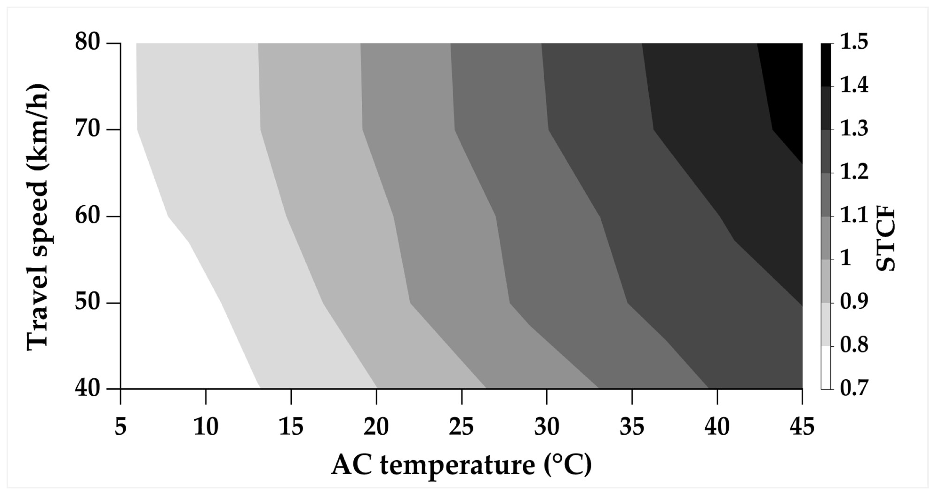
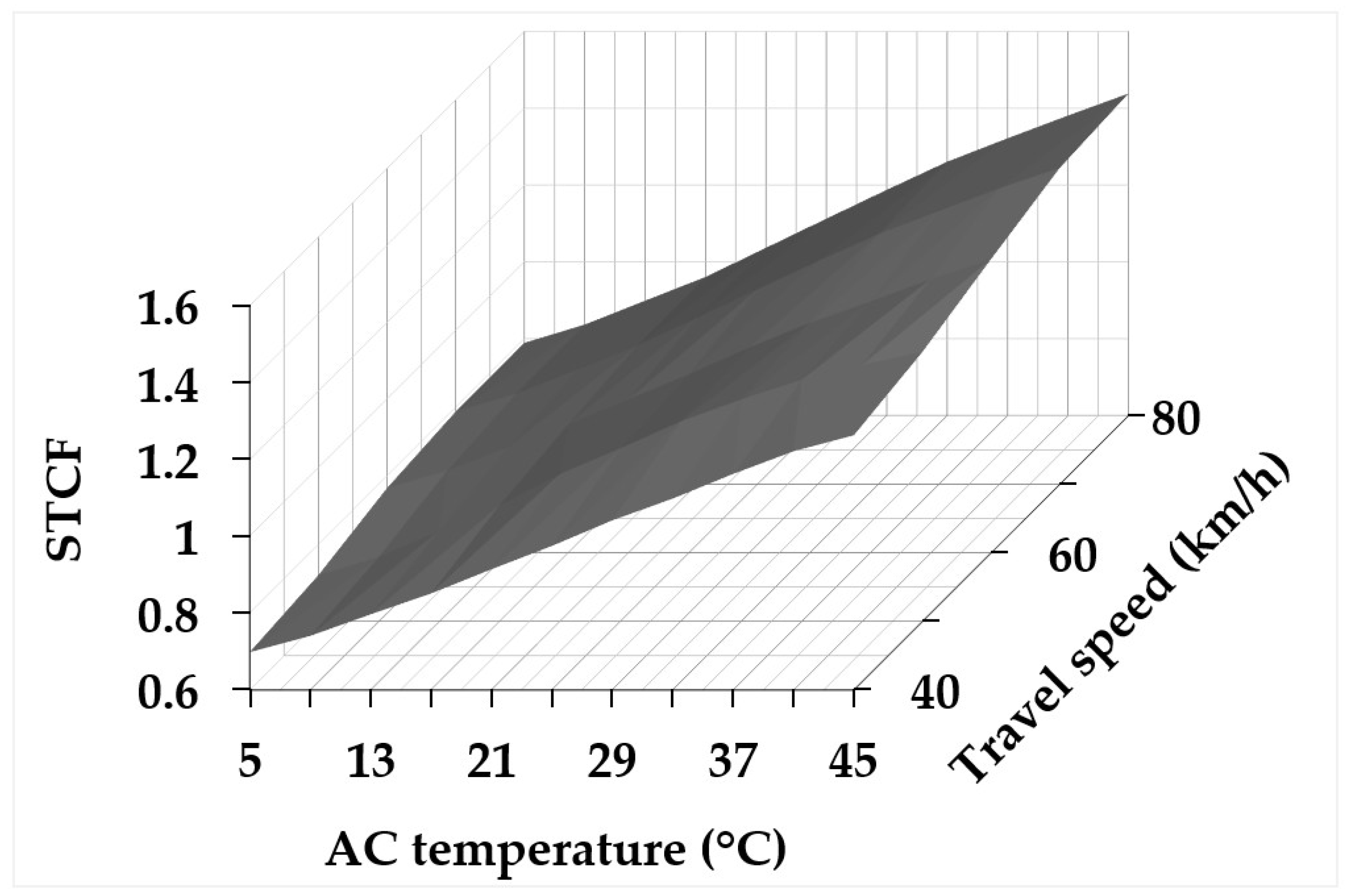
This part of the study involved correcting the deflection slopes for the combined effects of TSD travel speed and AC temperature. Deflection slopes obtained from FEM analyses, corresponding to each TSD travel speed ranging from 40 km/h to 80 km/h and AC temperatures ranging from 5 °C to 45 °C, were simultaneously corrected to a reference AC temperature of 21 °C and a reference TSD travel speed of 60 km/h using Equation (4), which defines the speed and temperature correction factor (STCF). As an example, Figure 13 presents a contour plot showing the relationship between STCF, AC temperature, and TSD travel speed at the offset distance of 600 mm from the centre of loading, with the AC thickness of 200 mm. Figure 14 provides a 3D representation of Figure 13, with AC temperature, travel speed, and STCF each represented on a separate axis in the 3D domain.
S T C F = D e f l e c t i o n   s l o p e   a t   a c t u a l   A C   t e m p e r a t u r e   a n d   a c t u a l   T S D   t r a v e l   s p e e d D e f l e c t i o n   s l o p e   a t   r e f e r e n c e   A C   t e m p e r a t u r e 21   ° C   a n d   r e f e r e n c e   T S D   t r a v e l   s p e e d   ( 60   k m / h )
As illustrated in Figure 14, the surface is nearly planar with minor curvature, indicating the suitability of a linear correlation between STCF, TSD travel speed, and AC temperature. Considering the results for other Doppler laser sensor locations and the AC layer’s thickness, Table 7 presents the corresponding linear regression equations and their MAPE values. As shown in Table 7, the MAPE values for the regression equations are mostly below 10%, indicating high accuracy in accordance with the criteria outlined in Table 3. However, the accuracy of the regression equations in predicting STCF at 100 mm offset distance from the centre of loading is lower, with the MAPE exceeding 10% at the AC thickness of 300 mm. This trend is consistent with the results presented in the previous section when predicting TCF for the deflection slopes. In that case, the linear equation was replaced with a parabolic polynomial to improve the regression fit. A similar approach was applied here, specifically for the regressions at the 100 mm offset distance from the centre of loading. A parabolic polynomial of AC temperature was added to the linear function of TSD travel speed to enhance the prediction of STCF. The revised regression equations and their corresponding MAPE values are presented in Table 8. As shown, the new fitted equations significantly improved the prediction of STCF, reducing the MAPE values notably.

4.5. Correlation Between Temperature Correction Factor and AC Thickness

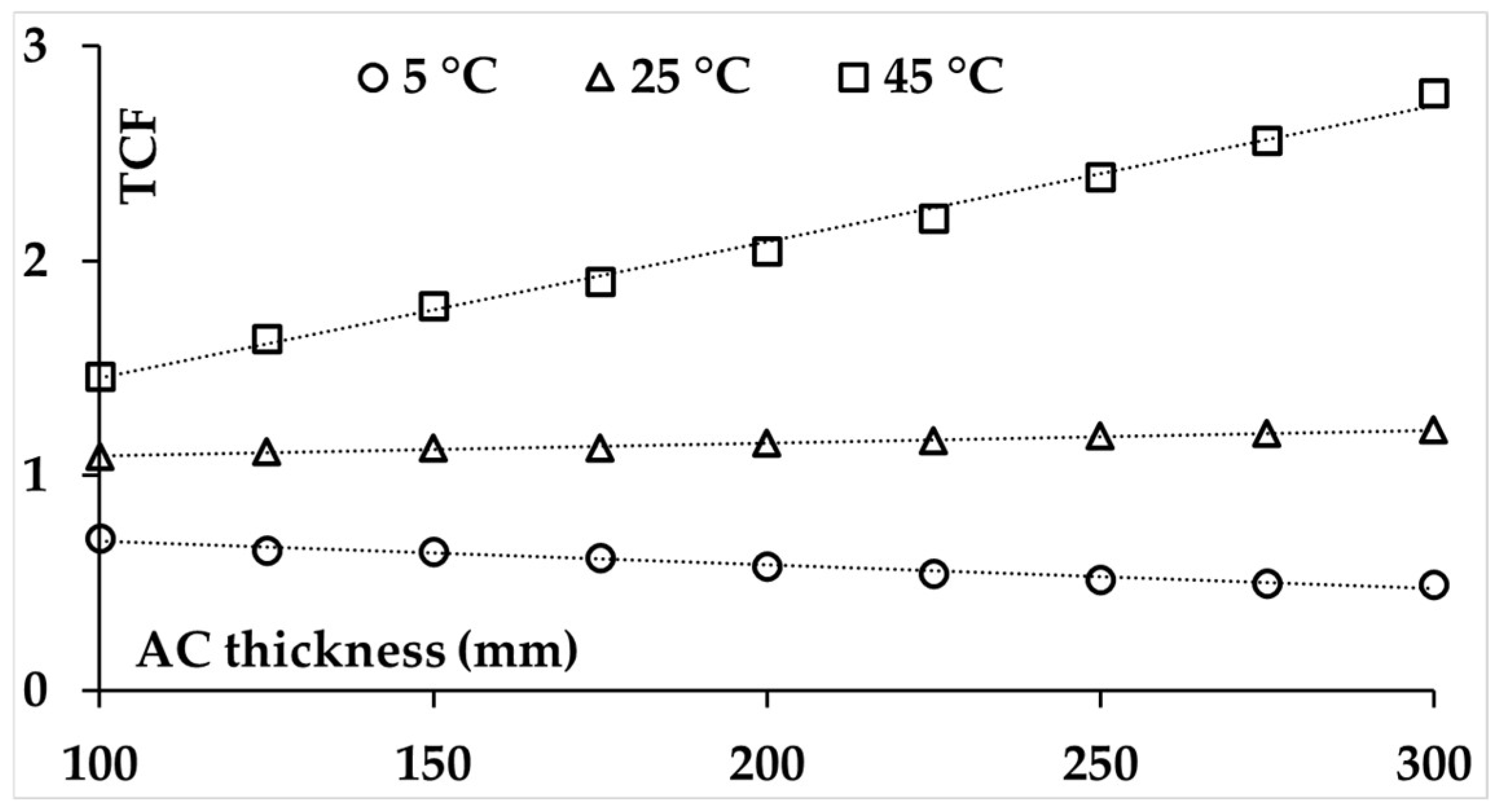
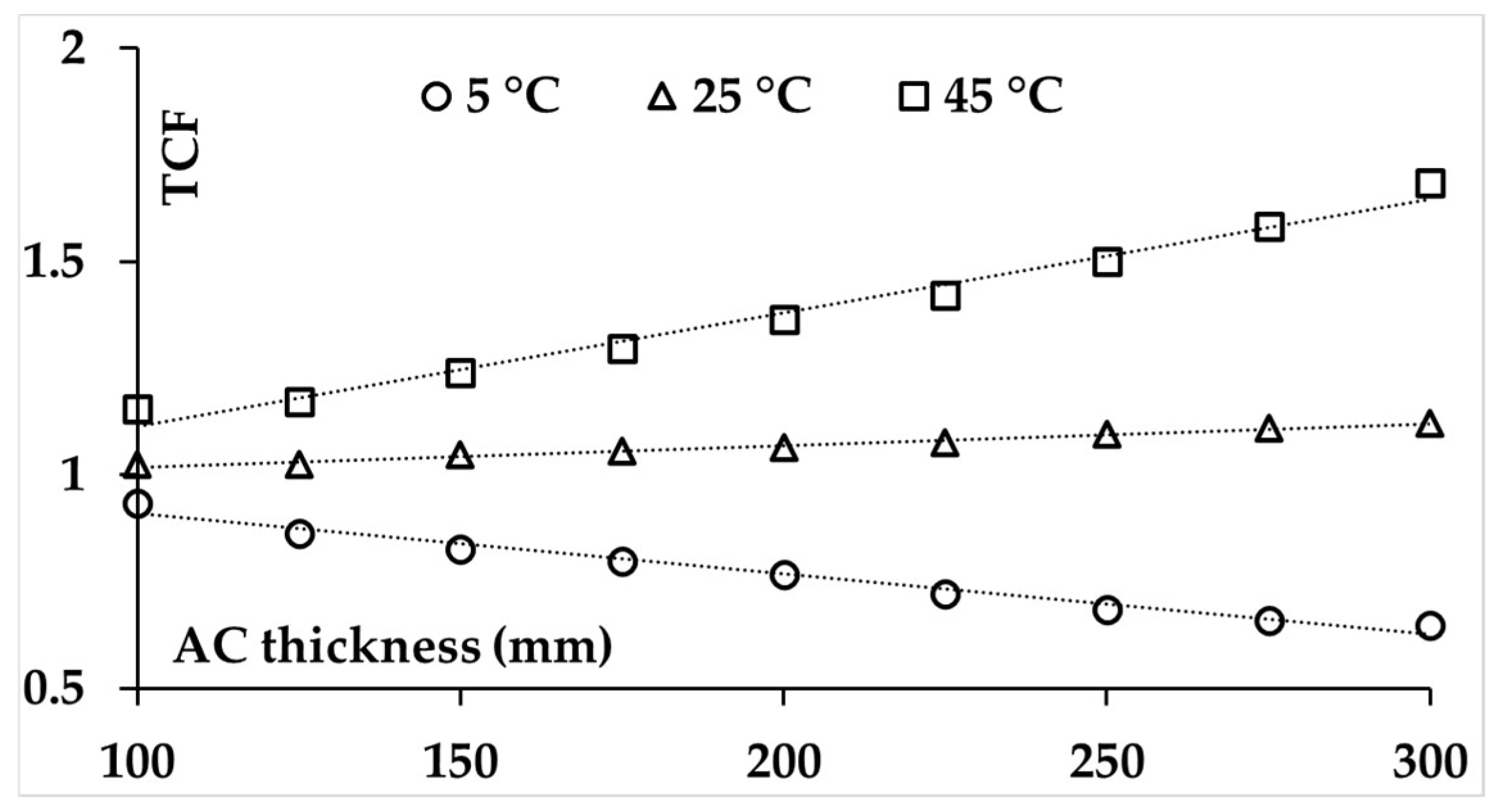
After examining how TSD travel speed and AC temperature influence deflection slopes and identifying trends to calculate correction factors, the effect of AC thickness on correction factors was also investigated. At this stage of the study, the focus was placed solely on temperature correction without including travel speed. This decision was based on earlier discussions about the possibility of controlling driving speed and the greater influence of AC temperature on deflection slopes. It also enabled the correlations between TCF and the AC layer’s thickness to be illustrated using simple graphs. The AC layer’s thickness varied from 100 mm to 300 mm in 25 mm increments, and three AC temperatures, 5, 25, and 45 °C, were considered in the analyses. The TSD travel speed was fixed at 60 km/h, and the reference temperature for calculating the TCF was set to 21 °C as previously used. Figure 15, Figure 16 and Figure 17 present the TCFs with respect to AC thickness at offset distances of 100, 600, and 1500 mm from the centre of loading, respectively. Table 9 presents the fitted linear regression equations along with their MAPE values. As can be seen, all MAPE values are below 2% and indicate accurate prediction of TCFs from AC thickness, based on the MAPE interpretation criteria shown in Table 3.

4.6. Simultaneous Speed and Temperature Correction Considering the AC Layer’s Thickness

Given the demonstrated accuracy of the linear relationship between TCF and the thickness of the AC layer, Equation (5) provides a general form for correcting deflection slopes by simultaneously accounting for AC temperature, TSD travel speed, and AC thickness. In this formulation, the coefficients can be expressed as functions f and g, which depend on AC temperature and TSD travel speed. As discussed earlier, these functions can be represented by a general form consisting of a parabolic polynomial of AC temperature and a linear function of TSD travel speed. However, for deflection slopes at 600 mm and 1500 mm offset distances from the centre of loading, the coefficient of the parabolic term for AC temperature can be set to zero, as a linear function of AC temperature provides sufficiently accurate predictions.
S T C F = f T , V × h + g T , V = a T 2 + b T + c V + d × h + ( m T 2 + n T + p V + q )
S T C F = a T 2 h + b T h + c V h + d h + m T 2 + n T + p V + q
T = AC temperature in °C;
V = TSD travel speed in km/h;
h = AC thickness in mm;
a , b , c , d , m , n , p , q = regression constants.
Table 10 presents the coefficients of the regression equations for STCF predictions, along with their corresponding MAPE values. The regressions were conducted using the outputs from a total of 495 FEM simulations, comprising 11 levels of AC temperature, 9 levels of AC layer’s thickness, and 5 levels of TSD travel speed (11 × 9 × 5 = 495). The prediction at the 100 mm offset distance from the centre of loading was performed twice, once including the parabolic term of AC temperature, and once considering only the linear term. As can be seen, all MAPE values are below 7%, indicating a high level of prediction accuracy.
The results in Table 10 illustrate that when developing correction factors for deflection slopes to account for AC temperature, AC thickness, and TSD travel speed at 100 mm offset distance from the centre of loading, including the parabolic term of AC temperature in the predictive equation resulted in lower prediction errors compared with using only the linear term. This finding is consistent with earlier findings of the study, which showed that at higher AC layer thicknesses, the parabolic term of AC temperature improves the prediction of correction factors. However, when all combinations of AC layer thicknesses were included in the regression analysis, it was found that even a linear term of AC temperature could provide accurate predictions, with a MAPE value of 6.5%. Based on these results, it is recommended that predictive equations for correction factors of deflection slopes at Doppler laser sensor locations near the centre of loading be developed separately for different categories of AC layer’s thickness. Specifically, the parabolic term of AC temperature should be used for higher AC layer thicknesses, while for lower to intermediate AC layer thicknesses, the linear term alone may be sufficient to simplify the form of the predictive equation.

5. Conclusions

Three-dimensional FEM simulations were conducted to model the rear axle of a TSD vehicle passing over a three-layer flexible pavement system. In the simulations, the AC temperature ranged from 5 °C to 45 °C, the AC thickness ranged from 100 mm to 300 mm, and the TSD travel speed varied from 40 km/h to 80 km/h. The objective was to derive correction factors to account for the effects of AC temperature and travel speed on deflection slopes at three offset distances from the centre of loading: 100 mm, which is close to the tyres; 600 mm, which represents a mid-distance location for Doppler laser sensors; and 1500 mm, which corresponds to the furthest Doppler laser sensor.
The findings showed that when only temperature effects were considered, while keeping the travel speed constant at 60 km/h, the temperature correction factor (TCF) could be estimated using linear correlations with AC temperature. For offset distances of 600 mm and 1500 mm, the Mean Absolute Percentage Error (MAPE) values for predictions were below 2.5% across different AC layer thicknesses. However, at 100 mm offset distance, linear correlations were less accurate, particularly at higher AC layer thicknesses, with MAPE values reaching up to 13%. The accuracy at this location improved significantly by using parabolic polynomial regression, reducing MAPE values to below 2%. Simultaneous correction of deflection slopes for both AC temperature and TSD travel speed showed similar trends. Linear regression using AC temperature and TSD travel speed accurately predicted the combined speed and temperature correction factor (STCF) at 600 mm and 1500 mm offset distances, with MAPE values for predictions below 3%. At 100 mm offset distance, the summation of a parabolic polynomial of AC temperature and a linear function of TSD travel speed resulted in STCF predictions with MAPE values below 2%. At the final stage of the study, it was found that TCF exhibits a linear correlation with AC thickness across different AC temperatures and different offset distances from the centre of loading, with MAPE values of the predictions below 2%. Consequently, predictive equations were developed to estimate the STCF at various offset distances from the centre of loading by accounting for the thickness of the AC layer, with resulting MAPE values remaining below 7%, demonstrating high accuracy. The results demonstrate the potential to develop regression equations that can predict correction factors for deflection slopes with high accuracy while accounting for variations in AC temperature and TSD travel speed.

6. Study Limitations and Path Towards Future Research

The following limitations exist in this study, and addressing them would broaden the findings and create opportunities for future research:
-
Only a limited number of pavement structures were evaluated, primarily to demonstrate the capability of developing correction factors for deflection slopes by accounting for AC temperature, travel speed, and AC thickness. It is recommended that future studies expand the FEM simulations to include a wider range of pavement structures by considering different material properties and layer thicknesses. This will help ensure that the regression equations with the developed structures are applicable to a broad spectrum of pavement configurations and can be extended to incorporate all relevant characteristics of pavement systems in terms of material properties and layer thicknesses. Expanding the range of pavement structures in future studies would require consideration of different aggregate gradations and bitumen types for the AC layer, resulting in different AC moduli, as well as varying base and subgrade layers’ moduli and AC and base layer thicknesses.
-
Some simplifications were made regarding the material properties of pavement layers. The temperature gradient within the AC layer was disregarded, and the AC layer was assumed to possess a uniform effective temperature throughout its entire thickness. The base and subgrade layers were considered to behave as linear elastic materials in the FEM simulations, with their nonlinear stress-dependent and cross-anisotropic behaviour neglected. The effect of moisture on subgrade stiffness was also not considered.
-
FEM simulations were performed using an equivalent circular loading simplification of a specific rear axle configuration for the TSD vehicle at the MnROAD facility, which limits the generality of the study findings. Furthermore, the effect of pavement surface roughness on the excitation of tyre load magnitude [43] was not considered.
-
Finally, although the range of AC temperatures considered in the study is relatively comprehensive, the findings could be further strengthened by including some negative AC temperatures in the FEM simulations. Additionally, considering a wider range of TSD travel speeds, particularly below 40 km/h and above 80 km/h, is important to enhance the comprehensiveness of the study.

Author Contributions

Conceptualisation, N.K. and M.S.; methodology, N.K. and M.S.; validation, N.K.; formal analysis, N.K.; investigation, N.K.; writing—original draft preparation, N.K.; writing—review and editing, M.S. and C.-L.L.; visualisation, N.K.; supervision, M.S. and C.-L.L. All authors have read and agreed to the published version of the manuscript.

Funding

This research received no external funding.

Data Availability Statement

The data presented in this study are available on request from the corresponding author.

Conflicts of Interest

The authors declare no conflicts of interest.

Abbreviations

The following abbreviations are used in this manuscript:
3DThree-Dimensional
AASHTOAmerican Association of State Highway and Transportation Officials
ACAsphalt Concrete
ANNArtificial Neural Network
FEAFinite Element Analysis
FEMFinite Element Method
FWDFalling Weight Deflectometer
MAEMean Absolute Error
MAPEMean Absolute Percentage Error
PGPerformance Grade
ReLURectified Linear Unit
SAFEMSemi-Analytical Finite Element Method
SCISurface Curvature Index
STCFSpeed and Temperature Correction Factor
TCFTemperature Correction Factor
TSDTraffic Speed Deflectometer
TSDDsTraffic Speed Deflection Devices
WLFWilliams–Landel–Ferry

References

  1. Kim, Y.R. Modeling of Asphalt Concrete; McGraw-Hill Education: Columbus, OH, USA, 2009; ISBN 978-0071464628. [Google Scholar]
  2. Lukanen, E.O.; Stubstad, R.; Briggs, R. Temperature Predictions and Adjustment Factors for Asphalt Pavement; Report No. FHWA-RD-98-085; Turner-Fairbank Highway Research Center, Federal Highway Administration, US Department of Transportation: McLean, VA, USA, 2000.
  3. Zhang, M.; Fu, G.; Ma, Y.; Xiao, R.; Huang, B. Speed and Temperature Superposition on Traffic Speed Deflectometer Measurements. Transp. Geotech. 2023, 40, 100990. [Google Scholar] [CrossRef]
  4. Guide for Design of Pavement Structures; American Association of State Highway and Transportation Officials (AASHTO): Washington, DC, USA, 1993.
  5. Ferne, B.W.; Langdale, P.; Round, N.; Fairclough, R. Development of a Calibration Procedure for the UK Highways Agency Traffic-Speed Deflectometer. Transp. Res. Rec. 2009, 2093, 111–117. [Google Scholar] [CrossRef]
  6. Rada, G.R.; Nazarian, S.; Visintine, B.A.; Siddharthan, R.; Thyagarajan, S. Pavement Structural Evaluation at the Network Level: Final Report; Report No. FHWA-HRT-15–074; Federal Highway Administration, US Department of Transportation: McLean, VA, USA, 2016.
  7. Shrestha, S.; Katicha, S.W.; Flintsch, G.W.; Thyagarajan, S. Application of Traffic Speed Deflectometer for Network-Level Pavement Management. Transp. Res. Rec. 2018, 2672, 348–359. [Google Scholar] [CrossRef]
  8. Nasimifar, M.; Chaudhari, S.; Thyagarajan, S.; Sivaneswaran, N. Temperature Adjustment of Surface Curvature Index from Traffic Speed Deflectometer Measurements. Int. J. Pavement Eng. 2020, 21, 1408–1418. [Google Scholar] [CrossRef]
  9. Siddharthan, R.V.; Yao, J.; Sebaaly, P.E. Pavement Strain from Moving Dynamic 3D Load Distribution. J. Transp. Eng. 1998, 124, 557–566. [Google Scholar] [CrossRef]
  10. Nasimifar, M.; Kamalizadeh, R.; Heidary, B. The Available Approaches for using Traffic Speed Deflectometer Data at Network Level Pavement Management System. Measurement 2022, 202, 111901. [Google Scholar] [CrossRef]
  11. Shen, K.; Wang, H.; Canestrari, F.; Graziani, A. Temperature Correction for Traffic Speed Deflectometer Measurements on Flexible Pavement using ANN Models. Road Mater. Pavement Des. 2025, 26 (Suppl. 1), 751–770. [Google Scholar] [CrossRef]
  12. Wu, C.; Wang, H.; Zhao, J.; Jiang, X.; Qiu, Y. Asphalt Pavement Modulus Backcalculation using Surface Deflections under Moving Loads. Comput.-Aided Civ. Infrastruct. Eng. 2020, 35, 1246–1260. [Google Scholar] [CrossRef]
  13. Wang, K.; Wei, J.; Hou, X.; Wu, C. Evaluation of Deflection Errors in Traffic Speed Deflectometer Measurements on Inverted Asphalt Pavement Structures. Appl. Sci. 2025, 15, 4059. [Google Scholar] [CrossRef]
  14. Tong, X.; Chen, Z.; Cheng, H.; Sun, L.; Li, Y.; Min, X.; Jin, F. Improved Deflection Calculation Methods for Traffic Speed Deflectometers for Asphalt Pavement Condition Assessments. Int. J. Pavement Eng. 2025, 26, 2498080. [Google Scholar] [CrossRef]
  15. ABAQUS; Dassault Systèmes Simulia Corp.: Johnston, RI, USA, 2022.
  16. Katicha, S.; Flintsch, G.; Diefenderfer, B. Ten Years of Traffic Speed Deflectometer Research in the United States: A Review. Transp. Res. Rec. 2022, 2676, 152–165. [Google Scholar] [CrossRef]
  17. TP 62-07; Standard Method of Test for Determining Dynamic Modulus of Hot Mix Asphalt (HMA). Standard Specifications for Transportation and Methods of Sampling and Testing. American Association of State Highway and Transportation Officials (AASHTO): Washington, DC, USA, 2009.
  18. Williams, M.L.; Landel, R.F.; Ferry, J.D. The Temperature Dependence of Relaxation Mechanisms in Amorphous Polymers and other Glass-forming Liquids. J. Am. Chem. Soc. 1955, 77, 3701–3707. [Google Scholar] [CrossRef]
  19. Park, S.; Schapery, R. Methods of Interconversion between Linear Viscoelastic Material Functions. Part I—A Numerical Method Based on Prony Series. Int. J. Solids Struct. 1999, 36, 1653–1675. [Google Scholar] [CrossRef]
  20. Pellinen, T.K.; Witczak, M.W.; Bonaquist, R.F. Asphalt Mix Master Curve Construction using Sigmoidal Fitting Function with Non-linear Least Squares Optimization. In Recent Advances in Materials Characterization and Modeling of Pavement Systems; Geotechnical Special Publication No. 12; American Society of Civil Engineers (ASCE): Reston, VA, USA, 2003; pp. 83–101. [Google Scholar] [CrossRef]
  21. ABAQUS 2016 Analysis User’s Guide Volume 3: Materials; Dassault Systèmes Simulia Corp.: Providence, RI, USA, 2015.
  22. Kim, S.; Kim, H. A New Metric of Absolute Percentage Error for Intermittent Demand Forecasts. Int. J. Forecast. 2016, 32, 669–679. [Google Scholar] [CrossRef]
  23. Lewis, C.D. Industrial and Business Forecasting Methods: A Practical Guide to Exponential Smoothing and Curve Fitting; Butterworth Scientific: Amsterdam, The Netherlands, 1982; ISBN 978-0408005593. [Google Scholar]
  24. Hu, X.; Li, J.; Hu, Y.; Sun, L. Study on Temperature Correction of Asphalt Pavement Deflection Based on the Deflection Change Rate. Appl. Sci. 2022, 13, 367. [Google Scholar] [CrossRef]
  25. Walia, A.; Rastogi, R.; Kumar, P.; Jain, S.S. Determination of Effective Depth to Measure Temperature Required for Structural Evaluation of Asphalt Pavements. J. Transp. Eng. Part B. Pavements 2021, 147, 04021040. [Google Scholar] [CrossRef]
  26. Inge, E.H., Jr.; Kim, Y.R. Prediction of Effective Asphalt Layer Temperature. In Transportation Research Record 1473; Transportation Research Board: Washington, DC, USA, 1995; pp. 93–100. [Google Scholar]
  27. Al-Qadi, I.L.; Wang, H.; Tutumluer, E. Dynamic Analysis of Thin Asphalt Pavements by using Cross-Anisotropic Stress-Dependent Properties for Granular Layer. Transp. Res. Rec. 2010, 2154, 156–163. [Google Scholar] [CrossRef]
  28. Brown, S.F.; Pappin, J. Analysis of Pavements with Granular Bases. In Transportation Research Record 810; Transportation Research Board: Washington, DC, USA, 1981; pp. 17–23. [Google Scholar]
  29. Tarefder, R.A.; Ahmed, M.U.; Rahman, A. Effects of Cross-Anisotropy and Stress-Dependency of Pavement Layers on Pavement Responses under Dynamic Truck Loading. J. Rock Mech. Geotech. Eng. 2016, 8, 366–377. [Google Scholar] [CrossRef]
  30. Uzan, J. Characterization of Granular Material. In Transportation Research Record 1022; Transportation Research Board: Washington, DC, USA, 1985; pp. 52–59. [Google Scholar]
  31. Kazemi, N.; Saleh, M.; Lee, C.-L. Effect of the Stress Dependency and Anisotropy of Unbound Granular Base and Subgrade Materials on TSD Deflection Slopes. In Proceedings of the International Conference on Transportation and Development (ICTD), Atlanta, GA, USA, 15–18 June 2024; pp. 327–337. [Google Scholar] [CrossRef]
  32. Kazemi, N.; Saleh, M.; Lee, C.-L. Effect of Nonlinear Stress-Dependency and Cross-Anisotropy on the Backcalculation Outputs from the TSD Deflection Slopes and the Effect on Estimated Pavement Performance. Int. J. Pavement Eng. 2024, 25, 2417967. [Google Scholar] [CrossRef]
  33. Lee, C.-L. Proportional Viscous Damping Model for Matching Damping Ratios. Eng. Struct. 2020, 207, 110178. [Google Scholar] [CrossRef]
  34. Carr, A.J.; Puthanpurayil, A.M.; Lavan, O.; Dhakal, R.P. Damping Models for Inelastic Time History Analysis: A Proposed Modelling Approach. In Proceedings of the 16th World Conference on Earthquake Engineering (WCEE), Santiago, Chile, 9–13 January 2017; Volume 11, pp. 7696–7705. [Google Scholar]
  35. Nasimifar, M.; Thyagarajan, S.; Sivaneswaran, N. Backcalculation of Flexible Pavement Layer Moduli from Traffic Speed Deflectometer Data. Transp. Res. Rec. 2017, 2641, 66–74. [Google Scholar] [CrossRef]
  36. Kannemeyer, L.; Lategan, W.; Mckellar, A. Verification of Traffic Speed Deflectometer Measurements using Instrumented Pavements in South Africa. In Proceedings of the Pavement Evaluation, Blacksburg, VA, USA, 15–18 September 2014. [Google Scholar]
  37. Elseifi, M.A.; Zihan, Z.U. Assessment of the Traffic Speed Deflectometer in Louisiana for Pavement Structural Evaluation; Report No. FHWA/LA/.18/590; Louisiana Transportation Research Center: Baton Rouge, LA, USA, 2018.
  38. ABAQUS 2016 User Subroutines Reference Guide; Dassault Systèmes Simulia Corp.: Providence, RI, USA, 2015.
  39. Fortran Compiler; Intel Corporation: Santa Clara, CA, USA, 2023.
  40. ABAQUS Theory Manual: Version 6.11; Dassault Systèmes Simulia Corp.: Providence, RI, USA, 2011.
  41. Wardle, L. CIRCLY and Mechanistic Pavement Design: The Past, Present and Towards the Future; Mincad Systems: Richmond, Australia, 2010. [Google Scholar]
  42. Uzan, J. JULEA (Jacob Uzan Layered Elastic Analysis); Technion University: Haifa, Israel, 1976. [Google Scholar]
  43. Marcondes, J.A.; Snyder, M.B.; Singh, S.P. Predicting Vertical Acceleration in Vehicles through Road Roughness. J. Transp. Eng. 1992, 118, 33–49. [Google Scholar] [CrossRef]
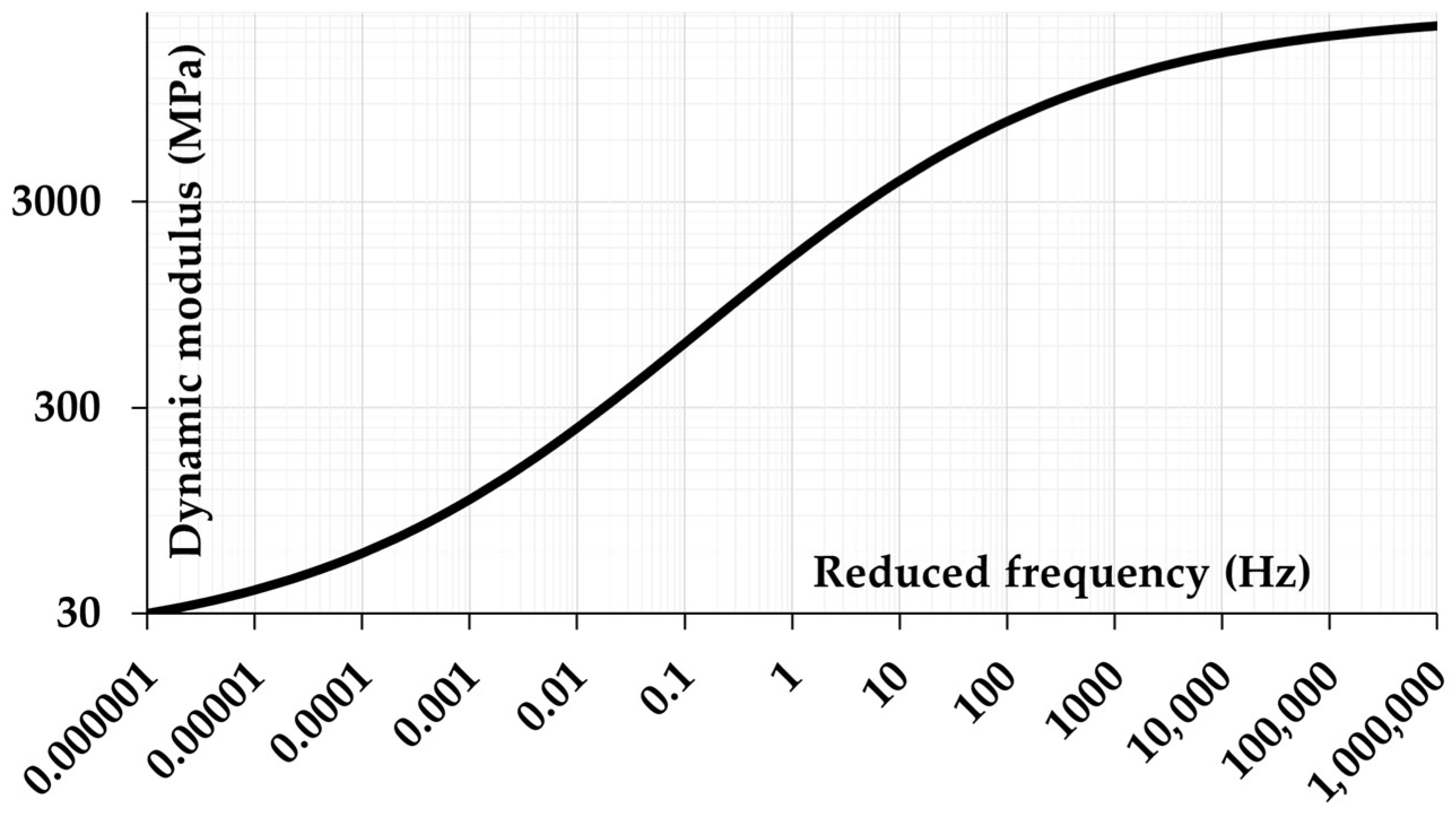
Figure 2. Dynamic modulus master curve of AC material at 29 °C.
Infrastructures 10 00351 g002
Figure 3. Dual tyre footprint loading configuration at each axle side (not to scale).
Infrastructures 10 00351 g003
Figure 4. Dual circular loading configuration at each axle side (not to scale).
Infrastructures 10 00351 g004
Figure 5. Three-dimensional half-pavement FEM model and mesh condition.
Infrastructures 10 00351 g005
Figure 6. Vertical surface deflections obtained from FEM, CIRCLY, and WinJULEA.
Infrastructures 10 00351 g006
Figure 7. Maximum critical tensile and compressive strains obtained from FEM and 3D-Move.
Infrastructures 10 00351 g007
Figure 8. Deflection slopes obtained from FEM analysis and field measurements.
Infrastructures 10 00351 g008
Figure 9. Linear regression over TCFs relative to AC temperature at 100 mm offset distance.
Infrastructures 10 00351 g009
Figure 10. Linear regression over TCFs relative to AC temperature at 600 mm offset distance.
Infrastructures 10 00351 g010
Figure 11. Linear regression over TCFs relative to AC temperature at 1500 mm offset distance.
Infrastructures 10 00351 g011
Figure 12. Parabolic regression over TCFs relative to AC temperature at 100 mm offset distance.
Infrastructures 10 00351 g012
Figure 13. Contour plot of STCFs at 600 mm offset distance and 200 mm AC thickness.
Infrastructures 10 00351 g013
Figure 14. Three-dimensional view of STCFs at 600 mm offset distance and 200 mm AC thickness.
Infrastructures 10 00351 g014
Figure 15. Linear regression over TCFs relative to AC thickness at 100 mm offset distance.
Infrastructures 10 00351 g015
Figure 16. Linear regression over TCFs relative to AC thickness at 600 mm offset distance.
Infrastructures 10 00351 g016
Figure 17. Linear regression over TCFs relative to AC thickness at 1500 mm offset distance.
Infrastructures 10 00351 g017
Table 1. Prony series parameters of AC14 mixture for ABAQUS input at 29 °C analysis.
i τ i (s) g i E0 (MPa)
110−60.00080218,403.1
210−50.207389
310−40.24844
410−30.246903
510−20.168632
610−10.081873
710.028347
8100.013771
91040.00001
101050.000011
111060.000011
τ i & g i = material constants for Prony series fitting; E0 = instantaneous Young’s modulus.
Table 2. MAPE values of Prony series fittings as well as WLF shifting function constants.
Reference Temperature (°C)MAPE (%) c 1 c 2 (°C)
53.117.9133.1
93.217.3137
133.116.8141.2
173.216.4145.2
213.115.9149.2
253.415.5153.2
293.215.1157.2
333.214.8161.3
373.314.4165.3
413.214169
453.213.7172.9
Table 3. Forecasting accuracy based on MAPE (data from [23]).
MAPEPrediction Accuracy
<10%High
10–20%Good
20–50%Reasonable
>50%Inaccurate
Table 4. Material properties and thicknesses of pavement layers in FEM simulations.
LayerThickness (mm)Modulus (MPa)Temperature (°C)Poisson’s RatioDensity (kg/m3)
AC100 to 300viscoelastic5 to 450.42300
Base300400-0.352000
SubgradeSemi-infinite50-0.452000
Table 5. Linear regression equations over TCFs relative to AC temperature.
Distance (mm)AC Thickness (mm)Regression EquationMAPE (%)
100100TCF = 0.02T * + 0.58911.2
200TCF = 0.0375T + 0.28055.2
300TCF = 0.0574T − 0.04613.2
600100TCF = 0.0056T + 0.89310.7
200TCF = 0.0154T + 0.68030.6
300TCF = 0.0274T + 0.45522.3
1500100TCF = 0.0018T + 0.970.7
200TCF = 0.0066T + 0.85340.6
300TCF = 0.014T + 0.70320.9
* T = AC temperature (°C).
Table 6. Parabolic regression equations over TCFs relative to AC temperature at 100 mm distance.
AC Thickness (mm)Regression EquationMAPE (%)
100TCF = −6 × 10⁻⁷T2 + 0.0201T * + 0.58881.2
200TCF = 0.0004T2 + 0.0172T + 0.46910.9
300TCF = 0.0011T2 + 0.0041T + 0.451.6
* T = AC temperature (°C).
Table 7. Linear regression equations over STCFs relative to AC temperature and travel speed.
Distance (mm)AC Thickness (mm)Regression EquationMAPE (%)
100100STCF = 0.02T * + 0.0013V * + 0.50341.3
200STCF = 0.038T + 0.0023V + 0.12315.9
300STCF = 0.0552T − 3 × 10⁻⁵V + 0.02712.6
600100STCF = 0.0058T + 0.0037V + 0.67251
200STCF = 0.0158T + 0.0034V + 0.46021.5
300STCF = 0.0262T + 0.0016V + 0.38832.9
1500100STCF = 0.0019T + 0.0075V + 0.48432.2
200STCF = 0.0061T + 0.0039V + 0.59482.4
300STCF = 0.0132T + 0.0013V + 0.61162.2
* T = AC temperature (°C); V = TSD travel speed (km/h).
Table 8. Parabolic regression equations over STCFs relative to AC temperature and travel speed at 100 mm offset distance.
AC Thickness (mm)Regression EquationMAPE (%)
100STCF = 4 × 10⁻⁵T2 + 0.0182T * + 0.0013V * + 0.52031.2
200STCF = 0.0004T2 + 0.0157T + 0.0023V + 0.33071.7
300STCF = 0.0011T2 + 0.0014T − 3 × 10⁻⁵V + 0.52731.9
* T = AC temperature (°C); V = TSD travel speed (km/h).
Table 9. Linear regression equations over TCFs relative to AC thickness.
Distance (mm)AC Temperature (°C)Regression EquationMAPE (%)
1005TCF = −0.0011h * + 0.80391.7
25TCF = 0.0006h + 1.03330.4
45TCF = 0.0064h + 0.81691.4
6005TCF = −0.0014h + 1.05121.7
25TCF = 0.0005h + 0.96830.4
45TCF = 0.0027h + 0.8461.6
15005TCF = −0.0011h + 1.09910.5
25TCF = 0.0003h + 0.97220.4
45TCF = 0.0013h + 0.90571.5
* h = AC thickness (mm).
Table 10. Regression equations over STCFs relative to temperature, travel speed, and AC thickness.
Offset Distance (mm)abcdmnpqMAPE (%)
100 (parabolic)4 × 10⁻⁶−3 × 10−52 × 10−5−2.4 × 10⁻³−3 × 10−40.0184−3 × 10−30.94023
100 (linear)02 × 10−4−6 × 10⁻⁶−2.4 × 10−300.00362.7 × 10−30.6726.5
600010−4−10−5−1.4 × 10⁻³⁰−0.00480.0050.77991.9
150006 × 10−5−3 × 10−56 × 10−40−0.00480.01030.45222.5
Disclaimer/Publisher’s Note: The statements, opinions and data contained in all publications are solely those of the individual author(s) and contributor(s) and not of MDPI and/or the editor(s). MDPI and/or the editor(s) disclaim responsibility for any injury to people or property resulting from any ideas, methods, instructions or products referred to in the content.