1. Introduction
Metaheuristic algorithms have become vital tools for addressing complex optimization problems and are widely applied in fields such as engineering design [
1,
2], machine learning [
3,
4], and control systems [
5,
6]. Compared to traditional mathematical optimization techniques, such as gradient-based techniques [
7], metaheuristics offer several advantages; they do not require gradient information, exhibit low sensitivity to initial conditions, and are well-suited for high-dimensional or multimodal problems [
8,
9]. Their flexibility in navigating the solution space and capability to avoid entrapment in local optima have made them a central focus in computational intelligence research [
10,
11].
In recent years, hybridization techniques have been increasingly employed to enhance the performance of metaheuristics by integrating complementary strategies from different algorithms, thereby improving the convergence speed, solution quality, and robustness [
12,
13,
14,
15]. Among these, particle swarm optimization (PSO) has received considerable attention due to its simplicity and rapid convergence [
16]. However, PSO also suffers from limited local exploitation ability and a tendency toward premature convergence. To mitigate these issues, numerous studies have combined particle swarm optimization (PSO) with evolutionary operators such as genetic algorithms (GA) [
17] and differential evolution (DE) [
18], adaptive parameter control techniques [
19], and multi-strategy perturbation schemes to better balance global exploration and local exploitation [
20].
In parallel, the ivy algorithm (IVYA) has emerged as a promising bio-inspired approach due to its straightforward design and strong local search capabilities [
21]. By mimicking the natural growth and propagation behaviors of ivy plants, IVYA can efficiently exploit the neighborhood of promising regions while preserving population diversity. Nevertheless, the lack of a global guidance mechanism limits its convergence efficiency on large-scale optimization problems.
Despite the development of various hybrid metaheuristics, most existing methods primarily focus on accelerating convergence or maintaining diversity, without effectively addressing how to preserve the exploration–exploitation balance while avoiding premature convergence. Moreover, mechanisms that adaptively adjust search strategies based on dynamic fitness landscapes remain underexplored in the current literature.
To bridge these gaps, this paper introduces a novel hybrid optimization algorithm—IVYPSO—which synergistically combines the global guidance of PSO with the adaptive local search capabilities of IVYA. IVYPSO incorporates a biologically inspired ivy perturbation variable (GV) into the PSO velocity update equation, enabling adaptive directional control and stochastic perturbations based on the current fitness landscape. This design enhances the algorithm’s ability to escape local optima while improving the population diversity and convergence stability. The main contributions of this work are summarized as follows:
A novel PSO-guided hybrid optimization algorithm, IVYPSO, is proposed. It embeds the ivy growth strategy of IVYA into the velocity update process of PSO, thereby enabling dynamic switching between local and global search modes.
A balanced search framework was constructed by comparing the fitness of the current individual with that of the global best. The algorithm dynamically determines whether to perform local exploitation or global exploration, thereby improving its adaptability to complex search spaces.
A comprehensive experimental evaluation was conducted on 26 standard benchmark functions and three constrained real-world engineering design problems. The performance of the proposed IVYPSO algorithm was compared against eleven advanced metaheuristic optimization algorithms, including classical methods (such as PSO, IVY, BOA, WOA, and GOOSE), as well as recently developed hybrid algorithms from high-quality research studies (including HPSOBOA, FDC-AGDE, dFDB-LSHADE, NSM-BO, dFDB-SFS, and FDB-AGSK). The experimental results demonstrate that IVYPSO consistently outperformed the compared algorithms in terms of optimization accuracy, convergence speed, and robustness.
The rest of this paper is organized as follows.
Section 2 reviews the related work concerning the design and development of metaheuristic search algorithms.
Section 3 introduces the PSO and ivy algorithms.
Section 4 presents the proposed IVYPSO hybrid algorithm.
Section 5 covers its testing on benchmark functions and applications for practical engineering problems.
Section 6 discusses the results and outlines future work.
2. Related Work
Metaheuristic algorithms have become essential tools for addressing complex, multimodal, and high-dimensional optimization problems. Inspired by natural, biological, or social phenomena, these gradient-free algorithms are particularly well-suited for real-world engineering applications. Recent advancements in metaheuristics have shifted the research focus toward enhancing the algorithmic performance by redesigning key components—namely, the guiding mechanisms, convergence strategies, and update schemes.
Among these components, the guiding mechanism is critical, as it governs how individuals or candidate solutions are influenced by others within the population. Traditional guidance approaches, such as those used in classical PSO, typically direct individuals toward global or local optima based on fitness values but often suffer from premature convergence and loss of population diversity. To address these challenges, advanced guiding strategies have been developed, including fitness distance balance (FDB) [
22], adaptive FDB (AFDB) [
23], dynamic FDB (DFDB) [
24], and fitness distance constraint (FDC). By incorporating spatial distance information between solutions, these methods achieve a more balanced trade-off between exploration and exploitation, as demonstrated by their successful integration into algorithms such as FDC_AGDE [
25], dFDB_LSHADE [
26], dFDB_SFS [
27], and FDB_AGSK [
28], which exhibit strong performance on benchmark functions and engineering problems.
Convergence strategies, which determine how candidate solutions are updated each iteration, also play a pivotal role in directing search trajectories and influencing the convergence speed. The contemporary approaches include time-decreasing control parameters, multi-phase convergence schemes, and hybrid deterministic random update models. For instance, the GOOSE algorithm adapts its convergence behavior across different search stages [
29], while HPSOBOA incorporates multiple convergence modes to sustain robustness across diverse problem domains [
30].
Moreover, update schemes—particularly for the selection of surviving individuals—are vital for maintaining the solution quality and population diversity. Conventional methods relying solely on fitness-based ranking risk stagnation and premature convergence. To overcome this, the natural survivor method (NSM) integrates the fitness performance with historical success rates to judiciously select individuals for the next generation [
31]. NSM has proven effective in algorithms such as NSM-BO and NSM-LSHADE-CnEpSin [
32], markedly enhancing the stability and global search performance in constrained engineering problems.
Despite these advances, most existing studies focus on improving individual algorithmic components—such as the convergence behavior or update strategies—often at the expense of overall adaptability or diversity. A unified framework that simultaneously integrates global guidance and bio-inspired local searches with dynamic adaptability remains lacking.
To bridge this gap, we propose a hybrid algorithm, IVYPSO, which synergistically combines PSO’s global search capability with the ivy algorithm’s local growth and diffusion mechanisms. By embedding a dynamic ivy-inspired variable GV within the PSO velocity update formula, IVYPSO adaptively switches search strategies based on individual fitness, effectively balancing exploration and exploitation. This design not only preserves the convergence accuracy but also enhances the robustness and diversity, offering a novel high-performance optimization framework tailored for complex global optimization challenges.
3. Materials and Methods
To better illustrate our hybrid algorithm, the inspiration behind and detailed implementation of the PSO algorithm and ivy algorithm will be introduced.
3.1. PSO Formulation
PSO is a nature-inspired swarm intelligence algorithm, proposed by Kennedy and Eberhart in 1995. Its core idea is based on simulating the foraging behavior of bird flocks or fish schools. By sharing information and collaborating among individuals, PSO strikes a balance between global exploration and local exploitation, effectively solving optimization problems.
In the PSO algorithm, each particle has a unique position and velocity , representing a potential solution. Here, , denotes the dimensionality of the search space. In each iteration, the position of the particle is dynamically updated based on the following three components:
- (1)
Inertia component: Determined by the particle’s previous velocity, it is used to maintain the particle’s movement trend and balance the global exploration capability of the search.
- (2)
Individual cognitive component: The particle adjusts its search direction based on its own historical best position , simulating individual learning behavior.
- (3)
Social component: The particle adjusts its direction based on the entire population’s global best position , reflecting social learning and collaborative effects.
During the search process, the particle’s position is influenced by its best position in the neighborhood and the global best position of the entire population.
The particle position and velocity update formulas are given by Equations (1) and (2), respectively:
where
is the inertia weight, which controls the balance between global and local searches;
and
are acceleration coefficients that determine the influence of individual and group learning, respectively;
and
are random numbers, ranging from 0 to 1, which enhance the randomness of the search.
The flowchart of the PSO algorithm is shown in
Figure 1.
3.2. IVYA Formulation
The ivy algorithm, derived from the growth behavior of ivy plants in nature, is a swarm intelligence optimization method. Ivy plants continuously grow, climb, and spread in the environment in search of sunlight, nutrients, and other resources for survival. This process serves as inspiration for addressing global optimization problems. The algorithm simulates the different life stages of ivy, including growth, ascent, and spreading [
33]. The algorithm’s implementation process can be outlined in the subsequent four steps:
- (1)
Initialize the population, where
and
represent the total number of members and the dimensionality of the problem, respectively. Thus, the
population member has the form
, where
, The total population of ivy plants is represented as
, At the start of the algorithm, the initial positions of the ivy algorithm population in the search space are determined using Equation (3):
where
represents a vector of dimension
with random numbers uniformly distributed in the range [0, 1]. The upper and lower limits of the search space are denoted by
and
, respectively, and
denotes the element-wise product of two vectors.
- (2)
Coordinated and disciplined population growth. In the growth process of the ivy algorithm, we assume that the growth rate
of the ivy algorithm is a function of time, expressed through a differential equation, as illustrated in Equation (4):
where
,
, and
represent the growth rate, growth velocity, and correction factor for growth deviation, respectively. The member
is modeled by Equation (5).
where
and
represent the growth rates at discrete time steps
and
, respectively;
is a random number in the range of [0, 1];
represents a random vector of dimension
.
- (3)
Obtaining sunlight for growth. For ivy in nature, quickly finding a surface to attach to is crucial. The movement towards the light source is modeled by Equations (6)–(8). In the proposed algorithm, this behavior is simulated by the
individual
in the population, selecting its closest and most optimal neighbor
(based on the value of the fitness function) as a reference for self-improvement, as shown in
Figure 2.
where
is a vector, with each component being the absolute value of the corresponding component in the vector
.
- (4)
Growth and evolution of ivy. After the member
navigates the search space globally to reach its nearest and most significant neighbor
, it enters a phase where
strives to directly follow the optimal member
in the population. This stage aligns with the pursuit of an improved optimal solution in the vicinity of
, as depicted in Equations (9) and (10).
The flowchart of the ivy algorithm is shown in
Figure 3.
4. Proposed Optimization Formulation of IVYPSO
The IVYPSO hybrid algorithm integrates the global exploration capability of PSO with the local exploitation and adaptive perturbation mechanism inspired by the natural growth behavior of ivy plants. Specifically, the algorithm leverages the PSO’s velocity-position update rule to guide individuals toward promising areas in the solution space. Meanwhile, an ivy-inspired introduces fine-grained random perturbations to enhance the local search capability around high-quality solutions. To balance exploration and exploitation, IVYPSO adaptively switches between global and local strategies based on a dynamic quality threshold. A greedy selection strategy is also employed to retain elite solutions in each iteration. This coordinated hybridization approach improves the convergence speed, avoids local optima, and enhances the solution’s overall accuracy.
4.1. Initialization Phase
In this phase, the objective function is defined to calculate the fitness. The lower and upper bounds of the search space, and , respectively, are set to restrict the solution range; individuals are randomly generated, and the position and velocity of each individual are initialized, along with the ivy variables. The specific parameter initialization process is as follows.
The particles’ initial positions in the search space are randomly generated, as described in Equation (11):
The velocity is initialized as a zero vector, as described in Equation (12):
The ivy growth variable
is then initialized, as described in Equation (13):
The ivy variable represents the relative growth behavior of an ivy plant within the bounded search space and is used to control the intensity of local random movement.
4.2. Guidance Mechanism: PSO-Guided Velocity Update
This step updates the velocity for each individual, as described by the velocity update formula in Equation (14):
where
,
,
,
, and
are randomly generated values within the interval [0, 1], adding randomness to the particles. This mechanism guides particles towards their personal best position
and the global best position
, promoting convergence toward high-quality areas.
This velocity update represents the guidance mechanism in a metaheuristic search (MHS), guiding particles toward personal and global best positions to balance exploration and exploitation. Recent state-of-the-art (SOTA) methods such as FDB and its variants improve the guidance by considering both the fitness and distance to avoid premature convergence.
4.3. Update Mechanism: Position Update with Ivy Perturbation
To achieve a dynamic balance between global and local searches, we introduce a dynamic control factor
, which is a dynamic adjustment parameter that controls the ratio between global and local search. The expression is as described in Equation (15):
The random value is in the range of [0, 1], and the value of dynamically changes, which helps introduce randomness and balance the strengths of global and local searches. By adjusting , the algorithm primarily focuses on global searches in the early stages and gradually enhances the local search capability in the later stages, thereby improving the convergence accuracy.
In each iteration, for each individual
the update strategy is selected based on the relationship between its current fitness value
and the global best fitness value
. The condition judgment formula is as described in Equation (16):
where
represents the fitness value of the current individual and
represents the fitness value of the current global best solution. If the condition is met, Equation (17) is used for local searches (exploited around a neighbor). Otherwise, Equation (18) is applied to global searches (perturbed toward the best). Equations (17) and (18) are as follows:
Here,
controls the perturbation magnitude;
is a normally distributed random value that mimics the irregular yet directed growth of ivy tips toward better areas. The ivy growth variable is then updated using Equation (19).
This adaptive update allows to decay or intensify based on the stochastic process, simulating flexible growth behaviors for refining solutions.
4.4. Survivor Selection Strategy
In metaheuristic search algorithms, survivor selection is a crucial component of the update mechanism that determines which individuals are retained in the population to balance the convergence speed and solution diversity. In IVYPSO, we employ a greedy selection strategy, described in Equation (20), to preserve improved solutions:
If the new position yields a better fitness than the current position , it replaces the current solution; otherwise, the original solution is retained. Additionally, the individual best and global best are updated synchronously upon improvement.
Furthermore, inspired by recent advances in metaheuristics, the NSM has been proposed as an effective survivor selection technique. NSM dynamically combines fitness and historical success information to select survivors, enhancing the stability and diversity in the population. Although IVYPSO does not explicitly implement NSM, its greedy selection strategy combined with ivy-inspired perturbations shares conceptual similarities with NSM’s goal of balancing exploitation and exploration, ensuring robustness against premature convergence. Future work may explore integrating NSM directly into IVYPSO to further improve the update mechanism performance.
4.5. Summary
Through PSO-guided global movement and ivy-inspired local perturbations, IVYPSO forms a complementary hybrid search system. The use of ivy growth variables enhances the adaptability and solution refinement, particularly in rugged or complex landscapes. The implementation process of IVYPSO is illustrated in
Figure 4 and Algorithm 1.
| Algorithm 1. IVYPSO |
| Input: N, Max_iteration, lb, ub, dim, fobj |
| Output: Destination_fitness, Destination_position, Convergence_curve |
| Initialize parameters: |
| Set PSO parameters: inertia weight (w), cognitive factor (c1), social factor (c2) |
| Initialize population size (N), maximum iterations (Max_iteration), search space (lb, ub) |
| Define and initialize the vine growth variable (GV) |
| Initialize population: |
| For each particle i in population: |
| Randomly initialize position Position_i within [lb, ub] |
| Initialize velocity Velocity_i as a zero vector |
| Evaluate fitness Cost_i = fobj(Position_i) |
| Initialize vine growth variable GV_i = Position_i/(ub - lb) |
| Set personal best PBest_i = Position_i and PBest_Cost_i = Cost_i |
| Set global best GBest as the particle with the lowest fitness value |
| Iteration loop (t = 1 to Max_iteration): |
| For each particle i in population: |
| Update velocity and position: |
| Generate random vectors r1 and r2 |
| Velocity_i = w * Velocity_i |
| + c1 * r1 * (PBest_i - Position_i) |
| + c2 * r2 * (GBest - Position_i) |
| Calculate dynamic control factor β: |
| β = 1 + (random/2) |
| Perform local or global search based on fitness comparison: |
| If Cost_i < β * GBest_Cost: |
| New_Position = Position_i |
| + |N(0,1)| * (Position_neighbor - Position_i) |
| + N(0,1) * GV_i |
| Else: |
| New_Position = GBest * (random + N(0,1) * GV_i) |
| Boundary handling: |
| Ensure New_Position is within [lb, ub] |
| Update vine growth variable: |
| GV_i = GV_i * (random^2 * N(0,1)) |
| Evaluate and update solutions: |
| New_Cost = fobj(New_Position) |
| If New_Cost < Cost_i: |
| Position_i = New_Position |
| Cost_i = New_Cost |
| If New_Cost < PBest_Cost_i: |
| PBest_i = New_Position |
| PBest_Cost_i = New_Cost |
| If New_Cost < GBest_Cost: |
| GBest = New_Position |
| GBest_Cost = New_Cost |
| Record the best fitness at the current iteration: |
| Convergence_curve(t) = GBest_Cost |
| Return: |
| Destination_fitness = GBest_Cost |
| Destination_position = GBest |
| Convergence_curve |
5. Results and Analytical Evaluation of the Experiment
To verify the proposed algorithm’s reliability and performance, 26 standard benchmark functions were utilized. Moreover, we applied the algorithm to three real-world engineering optimization problems to evaluate its practical performance. The subsequent sections offer comprehensive details on the benchmark functions, parameter configurations, and performance metrics. The algorithm’s effectiveness was assessed through a comparative analysis with ten widely recognized metaheuristic algorithms.
Setup for experiments: The proposed IVYPSO algorithm and other metaheuristic methods were implemented in MATLAB 2023a. All tests were conducted on a Windows 10 platform with an Intel(R) Core (TM) i9-14900KF processor (3.10 GHz) and 32 GB of RAM.
5.1. Global Optimization with 26 Benchmark Mathematical Test Functions
To assess the performance of the proposed IVYPSO algorithm in solving complex optimization problems, this study employed 26 widely recognized benchmark functions [
34,
35,
36]. These functions were selected to ensure a comprehensive evaluation covering various optimization scenarios, and they are grouped here into two main categories: unimodal and multimodal functions. Each function was tested in a 30-dimensional space.
Unimodal functions: The initial set of 15 benchmark functions (F1–F15) is unimodal, characterized by the presence of a single global optimum, making it suitable for evaluating the convergence speed and local exploitation capability of optimization algorithms. These functions provide a smooth search landscape without local optima, allowing the assessment of an algorithm’s ability to quickly converge to the global minimum.
For instance, the Quartic function introduces a noise component that simulates real-world measurement errors, making it relevant for applications such as experimental data fitting. The Sum Power function, with its amplified penalization of higher-order dimensions, reflects challenges seen in structural reliability or robust design tasks in engineering optimization.
Multimodal functions: The latter set of functions (F16–F26) is multimodal, containing numerous local optima and being employed to test an algorithm’s ability to maintain diversity and avoid premature convergence. These functions simulate complex landscapes typically encountered in real-world scenarios such as material design, resource allocation, or non-linear process optimization.
For example, the Alpine function represents rugged fitness landscapes with a repetitive pattern, akin to multi-peak phenomena in signal processing or energy system optimization. The Weierstrass function, characterized by its fractal-like structure, is often used to test algorithms under highly irregular and non-differentiable conditions, making it applicable to domains such as financial modeling or dynamic system tuning.
By adopting this comprehensive set of 26 benchmark functions, this study evaluated IVYPSO across a wide range of conditions, from simple landscapes to highly complex multimodal terrains. This thorough testing ensures that the algorithm’s effectiveness, robustness, and generalization ability were rigorously validated. The full mathematical formulations and parameter settings of the benchmark functions are detailed in
Table 1.
5.1.1. Performance Indicators
To objectively assess the effectiveness of the IVYPSO algorithm, this study used the following standard evaluation metrics to comprehensively assess its performance across different benchmark tests [
37,
38,
39,
40].
Average value (
): The average fitness value obtained from
independent runs of the algorithm, calculated as shown in Equation (21).
Standard deviation (
): The variability in the objective function values obtained from
independent runs of the algorithm. The standard deviation is calculated using Equation (22).
Best: The minimum fitness obtained from M independent runs of the algorithm, as shown in Equation (23).
where
denotes the optimal fitness value attained during run
.
5.1.2. Parameter Settings and Performance Comparison Against Other Algorithms
Table 2 summarizes the parameter settings for the IVYPSO algorithm and its comparison algorithms. The proper adjustment of the parameters for each algorithm is crucial to ensure optimal performance. To maintain the fairness of the comparison, the initial settings and common parameters for all algorithms are set based on the standard values from the existing literature, while the remaining parameters are optimized through experimental procedures. The comparison algorithms selected in this study include classic metaheuristic methods such as PSO, IVY, BOA [
41], and WOA [
42], as well as several recently proposed improved algorithms, including GOOSE and HPSOBOA, and several advanced variant algorithms such as FDC-AGDE, dFDB-LSHADE, NSM-BO, dFDB-SFS, and FDB-AGSK. These algorithms have demonstrated strong performance in the IEEE CEC competition and in solving real-world engineering optimization problems. In this study, the evaluation of the objective function is terminated upon reaching the maximum number of iterations.
5.1.3. Analysis of Numerical Results
The proposed algorithm’s performance was evaluated and compared with several mature and latest algorithms.
Table 3 presents a detailed comparison of the average fitness values and standard deviations achieved by the IVYPSO algorithm and other algorithms across the test functions. Notably, IVYPSO attained the best average fitness on 21 out of the 26 test functions (F1–F4, F6, F8–F20, F24–F26), outperforming the other 11 algorithms. Particularly impressive was its performance on 17 functions (F1–F4, F8, F9, F11, F13–F17, F19, F20, F24–F26), where it achieved the best average fitness with a standard deviation of zero, demonstrating excellent stability and efficiency. On functions F5, F21, and F23, the IVYPSO algorithm ranked 6th, 5th, and 4th, respectively. However, its performance on F7 and F22 was relatively poor, ranking 11th and 12th, respectively.
Table 4 compares the best fitness values obtained by the IVYPSO algorithm and the other 11 algorithms across the test functions. Among the 26 functions, IVYPSO achieved superior results on 20 functions (F1–F4, F8, F9, F11–F20, F24–F26), outperforming the other 11 algorithms. For functions F6, F21, and F23, IVYPSO ranked 2nd, 4th, and 2nd, respectively, in terms of the best fitness value. Nevertheless, its performance was inferior on functions F5, F7, and F22, where it ranked 8th, 11th, and 10th, respectively.
In summary, the IVYPSO algorithm can be considered a superior optimization algorithm.
5.1.4. Analysis of Convergence Behavior
Figure 5 compares the convergence behavior of the IVYPSO algorithm with that of other algorithms over 500 iterations. The vertical axis represents the best fitness value obtained at each iteration, while the horizontal axis indicates the iteration count. On 16 out of the 26 test functions (specifically F1–F4, F6, F8–F15, F18, F20, and F25), IVYPSO demonstrated consistently faster and more efficient convergence, outperforming the other algorithms. Although IVYPSO exhibits strong global optimization capability, a few other algorithms outperformed it in certain specific cases.
5.1.5. Analysis of Exploitation Capabilities
Ideal for evaluating the algorithm’s development capabilities, the single-modal benchmark functions (F1–F14) contain only one minimum. For functions F1–F4, F8, F9, F11, F13, and F14,
Figure 3 demonstrates that IVYPSO reaches the theoretical best solution in around 50 iterations. Reflecting IVYPSO’s high precision and stability,
Table 3 reveals that the average fitness and standard deviation for these functions are typically 0. These findings clearly indicate that IVYPSO outperforms most of the comparison algorithms on the benchmark functions. For the multi-modal functions F15–F17, F19, F20, and F24–F26, IVYPSO also attains the theoretical best fitness in around 50 iterations.
Table 4 demonstrates that the majority of the algorithms are capable of locating the theoretical optimal solution. Moreover,
Table 3 underscores that IVYPSO demonstrates better average fitness and standard deviation than most competing algorithms, highlighting its robust and stable exploration capabilities.
5.1.6. Wilcoxon Signed-Rank Analysis Results and Friedman Ranking Scores
To ensure statistically robust conclusions, the widely accepted Wilcoxon non-parametric [
43,
44,
45,
46] test was used to assess the effectiveness of IVYPSO compared to 11 other algorithms.
Table 5 presents the results of the Wilcoxon signed-rank test applied to 26 standard test functions at a significance level of α = 0.05, using the mean objective value of each function as the test sample. The
p-value, which reflects the significance level, is considered significant when below 0.05. The data in
Table 5 show that IVYPSO yields
p-values below 0.05 in all cases. Therefore, this analysis statistically validates the superiority of IVYPSO over the other 11 algorithms.
To evaluate further the overall performance of the proposed IVYPSO algorithm on the 26 benchmark functions, the Friedman scores were used to rank the average performances of 12 comparative algorithms [
47,
48,
49].
Table 6 presents the Friedman scores and their corresponding ranks. Among all algorithms, IVYPSO achieved the lowest Friedman score of 1.9231, ranking first, which demonstrates its outstanding performance across all test functions. In contrast, traditional algorithms such as PSO and BOA obtained Friedman scores of 5.8846 and 6.7308, ranking 9th and 11th, respectively, indicating relatively weaker overall performance. Similarly, some improved algorithms, such as FDC-AGDE and dFDB-LSHADE, ranked 12th and 10th, respectively, also underperforming compared to IVYPSO. These results indicate that IVYPSO exhibits strong robustness and competitiveness in solving complex optimization problems, and its overall performance surpasses that of both traditional and newly developed metaheuristic algorithms.
5.1.7. Analysis of Computational Expenses
The time complexity of the IVYPSO algorithm is primarily composed of three parts: the population initialization, iteration updates, and fitness evaluation. Let the population size be , the maximum number of iterations be , and the dimensionality of the decision variables be . In the population initialization phase, the random generation of each particle’s position and velocity, along with the fitness evaluation, requires a time complexity of . In each iteration, the algorithm updates the velocity and position of each particle, adjusts the ivy growth variables, and evaluates the fitness. The velocity and position updates involve basic vector operations, with a time complexity of , and the ivy growth variable update and random perturbation for local or global searches also have a time complexity of . The fitness evaluation is usually the most time-consuming operation. If the complexity of the objective function evaluation is , the fitness calculation for the entire population in each iteration has a time complexity of . Therefore, the overall time complexity of the IVYPSO algorithm can be expressed as . As the population size , maximum iteration count , and dimensionality increase, the algorithm’s time complexity grows linearly, making it suitable for large-scale, complex global optimization problems.
5.2. Application of IVYPSO to Engineering Optimization Problems
This section presents the application of the IVYPSO algorithm in solving engineering optimization problems that involve various inequality and equality constraints. For each optimization problem, IVYPSO was evaluated in 20 independent runs using a population size of 30 individuals, with a maximum of 500 iterations. The performance of IVYPSO was compared with 11 other algorithms, including PSO, IVY, BOA, WOA, GOOSE, HPSOBOA, FDC_AGDE, dFDB_LSHADE, NSM_BO, dFDB_SFS, and FDB_AGSK. Additionally, three stability analysis metrics were incorporated: SR, ACTs, and AFEs. SR represents the proportion of independent runs in which the algorithm successfully found solutions that satisfy all constraints and reach the global optimum or an acceptable level of precision. ACTs refers to the average time (in seconds) spent by the algorithm to complete each optimization task across multiple runs. AFEs indicates the average number of fitness function evaluations required to complete the optimization task over multiple experiments.
5.2.1. Gas Transmission Compressor Design (GTCD) Problem
Figure 6 illustrates the gas transmission compressor design (GTCD) problem, which is a representative and practical mechanical design case originally proposed by Beightler and Phillips [
50]. This problem involves determining the optimal values of several design variables, such as the pipeline length, inlet and outlet pressures, and pipe diameter, with the objective of minimizing the total cost of a gas pipeline transmission system while ensuring the delivery of 100 million cubic feet of natural gas per day.
The GTCD problem reflects a realistic and complex engineering scenario widely encountered in energy and process industries. It poses significant optimization challenges due to its non-linear, constrained, and multimodal nature. By applying the proposed IVYPSO algorithm to this problem, we aim to demonstrate its capability to handle real-world design constraints, achieve cost-effective solutions, and maintain robustness in practical optimization tasks. This problem has three decision variables: the length between two compressor stations; the compression ratio , at the compressor inlet, where , with being the pressure leaving the compressor station (psi) and being the pressure entering the compressor station (psi); and , the internal diameter of the pipeline (inches). The goal is to find the optimal values for , , and that minimize the value.
In this problem, the total annual cost of the gas transmission system is defined as in Equation (24):
where
,
,
, subject to:
Table 7 presents a comparison of the results for solving the gas transmission compressor design problem using IVYPSO and other algorithms from the literature. The success rate threshold for this problem was determined to be 1,677,759.2755. The best result achieved by IVYPSO was
,
,
, with a minimum cost of 1,677,759.2755 and with an SR value of 100%, which required minimal time to complete the task.
Table 8 shows a statistical analysis, showing that IVYPSO achieved the lowest average cost of 1,677,759.2755. These results demonstrate that compared to other optimization algorithms, IVYPSO delivers a superior solution to the gas transmission compressor design problem.
5.2.2. Three-Bar Truss Design Problem
Figure 7 shows the three-bar truss design problem. The three-bar truss is typically a simple planar truss structure composed of three rods forming a triangular shape. This problem is widely applicable in engineering design, particularly in the field of structural optimization. The design variables typically include the cross-sectional area or dimensions of the rods, with the objective of minimizing the total mass of the truss while ensuring compliance with stress and geometric constraints. Such problems effectively reflect real-world engineering demands for structural safety and material efficiency, making them commonly used as benchmark problems for evaluating the performance of optimization algorithms.
The total mass of the three-bar truss can be expressed by Equation (25):
where
,
:
where
.
Table 9 presents a comparison of the results for solving the three-bar truss design problem using IVYPSO and other algorithms from the literature. The success rate threshold for this problem was determined to be 263.8523. The best result obtained by IVYPSO was
,
, with a minimum cost of 263.8523 and an SR value of 100%, and it required minimal time to complete the task.
Table 10 provides a statistical analysis, showing that IVYPSO achieved the lowest average cost of 263.8523. These results indicate that compared to other optimization algorithms, IVYPSO provides a better solution for the three-bar truss design problem.
5.2.3. Multiple-Disk Clutch Brake Design Problem
Figure 8 illustrates the multiple-disk clutch brake design problem, a classic engineering optimization issue that is commonly encountered in automation equipment, mechanical transmission systems, and the automotive industry [
51]. This problem involves optimizing the design of the clutch and brake system to minimize the stopping time of the brake while ensuring high operational efficiency and stability. Such design problems are highly relevant to real-world engineering scenarios, where the balance between performance, efficiency, and reliability is critical. By addressing this problem, the algorithm’s ability to handle practical engineering challenges and improve the overall system design is demonstrated, reflecting its applicability in real-world applications. This problem involves five decision variables: the inner radius
in millimeters, outer radius
in millimeters, disk thickness
in millimeters, driving force
, and number of friction surfaces
.
The brake’s stopping time can be expressed by Equation (26):
where
,
,
,
,
, subject to:
where:
Table 11 presents a comparison of the results for solving the multiple-disk clutch brake design problem using IVYPSO and other algorithms from the literature. The success rate threshold for this problem was determined to be 0.2352. The best result obtained by IVYPSO was
,
,
,
,
, with the lowest cost of 0.2352 and an SR value of 100%, and it required minimal time to complete the task.
Table 12 shows a statistical analysis, showing that IVYPSO achieves the lowest average cost of 0.2352. These results indicate that compared to other optimization algorithms, IVYPSO provides a better solution for the multiple-disk clutch brake design problem.
6. Conclusions
The proposed IVYPSO algorithm effectively enhances both the global exploration and local exploitation capabilities within complex search spaces by integrating ivy growth variables and dynamic control factors into the classical PSO framework. The ivy growth variables facilitate diverse search behaviors that prevent premature convergence, while the dynamic control factors adaptively balance the emphasis between global and local searches based on fitness evaluations.
Extensive experiments on 26 benchmark functions and three challenging engineering optimization problems—including the multiple-disk clutch brake design and gas transmission compressor design—demonstrated that IVYPSO achieves superior solution quality with rapid convergence. Comparative analyses against ten state-of-the-art optimization algorithms further confirmed the algorithm’s superiority in convergence accuracy, stability, and robustness, particularly in handling multi-modal and high-dimensional problems where the global optimization ability is critical.
This study lays a foundation for further research in several directions. Our future work will focus on extending IVYPSO to more complex engineering problems and multi-objective optimization scenarios, especially those involving dynamic, multi-modal, and high-dimensional environments. Moreover, the incorporation of adaptive parameter tuning strategies is planned to optimize the design of ivy growth variables and dynamic control factors, thereby improving the algorithm’s flexibility and performance across diverse problem domains.
In addition, hybridizing IVYPSO with other intelligent optimization techniques, such as genetic algorithms, differential evolution, and simulated annealing, to build multi-fusion frameworks may offer significant performance enhancements. This would leverage complementary algorithmic strengths and further improve the solution quality and convergence behavior.
Author Contributions
Conceptualization, K.Z. and F.Y.; methodology, K.Z. and Y.J.; software, Y.J. and Z.Z.; validation, Y.J. and Z.Z.; formal analysis, F.Y.; investigation, K.Z. and Z.Z.; data curation, Y.J.; writing—original draft preparation, K.Z.; writing—review and editing, Z.M. and Y.P.; supervision, F.Y.; project administration, F.Y. All authors have read and agreed to the published version of the manuscript.
Funding
This research received no external funding.
Institutional Review Board Statement
Not applicable.
Informed Consent Statement
Not applicable.
Data Availability Statement
The datasets used and/or analyzed during the current study are publicly available and can be accessed without any restrictions. If needed, they can also be obtained by contacting the corresponding author.
Acknowledgments
This work was supported by equipment funded through the Intelligent Connected New Energy Vehicle Teaching System project of Chongqing University of Technology, under the national initiative “Promote Large-Scale Equipment Renewals and Trade-Ins of Consumer Goods”.
Conflicts of Interest
The authors declare no conflict of interest. The authors declare that they have no known competing financial interests or personal relationships that could have appeared to influence the work reported in this paper.
References
- Sattar, D.; Salim, R. A smart metaheuristic algorithm for solving engineering problems. Eng. Comput. 2021, 37, 2389–2417. [Google Scholar] [CrossRef]
- Abualigah, L.; Elaziz, M.A.; Khasawneh, A.M.; Alshinwan, M.; Ibrahim, R.A.; Al-Qaness, M.A.A.; Mirjalili, S.; Sumari, P.; Gandomi, A.H. Meta-heuristic optimization algorithms for solving real-world mechanical engineering design problems: A comprehensive survey, applications, comparative analysis, and results. Neural Comput. Appl. 2022, 34, 4081–4110. [Google Scholar] [CrossRef]
- Talbi, E.G. Machine learning into metaheuristics: A survey and taxonomy. ACM Comput. Surv. (CSUR) 2021, 54, 1–32. [Google Scholar] [CrossRef]
- Kaveh, M.; Mesgari, M.S. Application of meta-heuristic algorithms for training neural networks and deep learning architectures: A comprehensive review. Neural Process. Lett. 2023, 55, 4519–4622. [Google Scholar] [CrossRef] [PubMed]
- Katebi, J.; Shoaei-Parchin, M.; Shariati, M.; Trung, N.T.; Khorami, M. Developed comparative analysis of metaheuristic optimization algorithms for optimal active control of structures. Eng. Comput. 2020, 36, 1539–1558. [Google Scholar] [CrossRef]
- Joseph, S.B.; Dada, E.G.; Abidemi, A.; Oyewola, D.O.; Khammas, B.M. Metaheuristic algorithms for PID controller parameters tuning: Review, approaches and open problems. Heliyon 2022, 8, e09399. [Google Scholar] [CrossRef]
- Ahmadianfar, I.; Bozorg-Haddad, O.; Chu, X. Gradient-based optimizer: A new metaheuristic optimization algorithm. Inf. Sci. 2020, 540, 131–159. [Google Scholar] [CrossRef]
- Abdel-Basset, M.; Mohamed, R.; Elkomy, O.M.; Abouhawwash, M. Recent metaheuristic algorithms with genetic operators for high-dimensional knapsack instances: A comparative study. Comput. Ind. Eng. 2022, 166, 107974. [Google Scholar] [CrossRef]
- Keivanian, F.; Chiong, R. A novel hybrid fuzzy–metaheuristic approach for multimodal single and multi-objective optimization problems. Expert Syst. Appl. 2022, 195, 116199. [Google Scholar] [CrossRef]
- Huang, Y.; Lu, S.; Liu, Q.; Han, T.; Li, T. GOHBA: Improved Honey Badger Algorithm for Global Optimization. Biomimetics 2025, 10, 92. [Google Scholar] [CrossRef]
- Zhu, X.; Zhang, J.; Jia, C.; Liu, Y.; Fu, M. A Hybrid Black-Winged Kite Algorithm with PSO and Differential Mutation for Superior Global Optimization and Engineering Applications. Biomimetics 2025, 10, 236. [Google Scholar] [CrossRef] [PubMed]
- Choi, K.; Jang, D.-H.; Kang, S.-I.; Lee, J.-H.; Chung, T.-K.; Kim, H.-S. Hybrid algorithm combing genetic algorithm with evolution strategy for antenna design. IEEE Trans. Magn. 2015, 52, 7209004. [Google Scholar] [CrossRef]
- Yu, X.; Jiang, N.; Wang, X.; Li, M. A hybrid algorithm based on grey wolf optimizer and differential evolution for UAV path planning. Expert Syst. Appl. 2023, 215, 119327. [Google Scholar] [CrossRef]
- Peng, Y.; Wang, Y.; Hu, F.; He, M.; Mao, Z.; Huang, X.; Ding, J. Predictive modeling of flexible EHD pumps using Kolmogorov–Arnold Networks. Biomim. Intell. Robot. 2024, 4, 100184. [Google Scholar] [CrossRef]
- Mao, Z.; Bai, X.; Peng, Y.; Shen, Y. Design, modeling, and characteristics of ring-shaped robot actuated by functional fluid. J. Intell. Mater. Syst. Struct. 2024, 35, 1459–1470. [Google Scholar] [CrossRef]
- Kennedy, J.; Eberhart, R. Particle swarm optimization. In Proceedings of the ICNN’95-International Conference on Neural Networks, Perth, Australia, 27 November–1 December 1995; IEEE: Piscataway, NJ, USA, 1995; Volume 4, pp. 1942–1948. [Google Scholar]
- Papazoglou, G.; Biskas, P. Review and comparison of genetic algorithm and particle swarm optimization in the optimal power flow problem. Energies 2023, 16, 1152. [Google Scholar] [CrossRef]
- Thangaraj, R.; Pant, M.; Abraham, A.; Bouvry, P. Particle swarm optimization: Hybridization perspectives and experimental illustrations. Appl. Math. Comput. 2011, 217, 5208–5226. [Google Scholar] [CrossRef]
- Sun, J.; Xu, W.; Feng, B. Adaptive parameter control for quantum-behaved particle swarm optimization on individual level. In Proceedings of the 2005 IEEE International Conference on Systems, Man and Cybernetics, Waikoloa, HI, USA, 12 October 2015; IEEE: Piscataway, NJ, USA, 2005; Volume 4, pp. 3049–3054. [Google Scholar]
- Song, Y.; Liu, Y.; Chen, H.; Deng, W. A multi-strategy adaptive particle swarm optimization algorithm for solving optimization problem. Electronics 2023, 12, 491. [Google Scholar] [CrossRef]
- Ghasemi, M.; Zare, M.; Trojovský, P.; Rao, R.V.; Trojovská, E.; Kandasamy, V. Optimization based on the smart behavior of plants with its engineering applications: Ivy algorithm. Knowl. Based Syst. 2024, 295, 111850. [Google Scholar] [CrossRef]
- Kahraman, H.T.; Aras, S.; Gedikli, E. Fitness-distance balance (FDB): A new selection method for meta-heuristic search algorithms. Knowl. Based Syst. 2020, 190, 105169. [Google Scholar] [CrossRef]
- Duman, S.; Kahraman, H.T.; Kati, M. Economical operation of modern power grids incorporating uncertainties of renewable energy sources and load demand using the adaptive fitness-distance balance-based stochastic fractal search algorithm. Eng. Appl. Artif. Intell. 2023, 117, 105501. [Google Scholar] [CrossRef]
- Kahraman, H.T.; Bakir, H.; Duman, S.; Katı, M.; Aras, S.; Guvenc, U. Dynamic FDB selection method and its application: Modeling and optimizing of directional overcurrent relays coordination. Appl. Intell. 2022, 52, 4873–4908. [Google Scholar] [CrossRef]
- Ozkaya, B.; Kahraman, H.T.; Duman, S.; Guvenc, U. Fitness-Distance-Constraint (FDC) based guide selection method for constrained optimization problems. Appl. Soft Comput. 2023, 144, 110479. [Google Scholar] [CrossRef]
- Yildirim, I.; Bozkurt, M.H.; Kahraman, H.T.; Aras, S. Dental X-Ray image enhancement using a novel evolutionary optimization algorithm. Eng. Appl. Artif. Intell. 2025, 142, 109879. [Google Scholar] [CrossRef]
- Kahraman, H.T.; Hassan, M.H.; Katı, M.; Tostado-Véliz, M.; Duman, S.; Kamel, S. Dynamic-fitness-distance-balance stochastic fractal search (dFDB-SFS algorithm): An effective metaheuristic for global optimization and accurate photovoltaic modeling. Soft Comput. 2024, 28, 6447–6474. [Google Scholar] [CrossRef]
- Bakır, H.; Duman, S.; Guvenc, U.; Kahraman, H.T. Improved adaptive gaining-sharing knowledge algorithm with FDB-based guiding mechanism for optimization of optimal reactive power flow problem. Electr. Eng. 2023, 105, 3121–3160. [Google Scholar] [CrossRef]
- Hamad, R.K.; Rashid, T.A. GOOSE algorithm: A powerful optimization tool for real-world engineering challenges and beyond. Evol. Syst. 2024, 15, 1249–1274. [Google Scholar] [CrossRef]
- Zhang, M.; Long, D.; Qin, T.; Yang, J. A chaotic hybrid butterfly optimization algorithm with particle swarm optimization for high-dimensional optimization problems. Symmetry 2020, 12, 1800. [Google Scholar] [CrossRef]
- Kahraman, H.T.; Katı, M.; Aras, S.; Taşci, D.A. Development of the Natural Survivor Method (NSM) for designing an updating mechanism in metaheuristic search algorithms. Eng. Appl. Artif. Intell. 2023, 122, 106121. [Google Scholar] [CrossRef]
- Öztürk, H.T.; Kahraman, H.T. Metaheuristic search algorithms in Frequency Constrained Truss Problems: Four improved evolutionary algorithms, optimal solutions and stability analysis. Appl. Soft Comput. 2025, 171, 112854. [Google Scholar] [CrossRef]
- Ouyang, H.; Li, W.; Gao, F.; Huang, K.; Xiao, P. Research on Fault Diagnosis of Ship Diesel Generator System Based on IVY-RF. Energies 2024, 17, 5799. [Google Scholar] [CrossRef]
- Jamil, M.; Yang, X.S. A literature survey of benchmark functions for global optimisation problems. Int. J. Math. Model. Numer. Optim. 2013, 4, 150–194. [Google Scholar] [CrossRef]
- Zhan, Z.-H.; Shi, L.; Tan, K.C.; Zhang, J. A survey on evolutionary computation for complex continuous optimization. Artif. Intell. Rev. 2022, 55, 59–110. [Google Scholar] [CrossRef]
- Cai, T.; Zhang, S.; Ye, Z.; Zhou, W.; Wang, M.; He, Q.; Chen, Z.; Bai, W. Cooperative metaheuristic algorithm for global optimization and engineering problems inspired by heterosis theory. Sci. Rep. 2024, 14, 28876. [Google Scholar] [CrossRef]
- Mao, Z.; Hosoya, N.; Maeda, S. Flexible electrohydrodynamic fluid-driven valveless water pump via immiscible interface. Cyborg Bionic Syst. 2024, 5, 0091. [Google Scholar] [CrossRef]
- Lau, S.L.H.; Lim, J.; Chong, E.K.P.; Wang, X. Single-pixel image reconstruction based on block compressive sensing and convolutional neural network. Int. J. Hydromechatronics 2023, 6, 258–273. [Google Scholar] [CrossRef]
- Verma, H.; Siruvuri, S.V.; Budarapu, P.R. A machine learning-based image classification of silicon solar cells. Int. J. Hydromechatronics 2024, 7, 49–66. [Google Scholar] [CrossRef]
- Alawi, O.A.; Kamar, H.M.; Shawkat, M.M.; Al Ani, M.M.; Mohammed, H.A.; Homod, R.Z.; Wahid, M.A. Artificial intelligence-based viscosity prediction of polyalphaolefin-boron nitride nanofluids. Int. J. Hydromechatro. 2024, 7, 89–112. [Google Scholar] [CrossRef]
- Arora, S.; Singh, S. Butterfly optimization algorithm: A novel approach for global optimization. Soft Comput. 2019, 23, 715–734. [Google Scholar] [CrossRef]
- Mirjalili, S.; Lewis, A. The whale optimization algorithm. Adv. Eng. Softw. 2016, 95, 51–67. [Google Scholar] [CrossRef]
- Yuan, F.; Huang, X.; Zheng, L.; Wang, L.; Wang, Y.; Yan, X.; Gu, S.; Peng, Y. The Evolution and Optimization Strategies of a PBFT Consensus Algorithm for Consortium Blockchains. Information 2025, 16, 268. [Google Scholar] [CrossRef]
- Zhang, C.; Chen, J.; Li, J.; Peng, Y.; Mao, Z. Large language models for human–robot interaction: A review. Biomim. Intell. Robot. 2023, 3, 100131. [Google Scholar] [CrossRef]
- Peng, Y.; Yang, X.; Li, D.; Ma, Z.; Liu, Z.; Bai, X.; Mao, Z. Predicting flow status of a flexible rectifier using cognitive computing. Expert Syst. Appl. 2025, 264, 125878. [Google Scholar] [CrossRef]
- Bai, X.; Peng, Y.; Li, D.; Liu, Z.; Mao, Z. Novel soft robotic finger model driven by electrohydrodynamic (EHD) pump. J. Zhejiang Univ. Sci. A 2024, 25, 596–604. [Google Scholar] [CrossRef]
- Mao, Z.; Peng, Y.; Hu, C.; Ding, R.; Yamada, Y.; Maeda, S. Soft computing-based predictive modeling of flexible electrohydrodynamic pumps. Biomim. Intell. Robot. 2023, 3, 100114. [Google Scholar] [CrossRef]
- Peng, Y.; Sakai, Y.; Funabora, Y.; Yokoe, K.; Aoyama, T.; Doki, S. Funabot-Sleeve: A Wearable Device Employing McKibben Artificial Muscles for Haptic Sensation in the Forearm. IEEE Robot. Autom. Lett. 2025, 10, 1944–1951. [Google Scholar] [CrossRef]
- Mao, Z.; Kobayashi, R.; Nabae, H.; Suzumori, K. Multimodal strain sensing system for shape recognition of tensegrity structures by combining traditional regression and deep learning approaches. IEEE Robot. Autom. Lett. 2024, 9, 10050–10056. [Google Scholar] [CrossRef]
- Dai, L.; Zhang, L.; Chen, Z. GrS Algorithm for Solving Gas Transmission Compressor Design Problem. In Proceedings of the 2022 IEEE/WIC/ACM International Joint Conference on Web Intelligence and Intelligent Agent Technology (WI-IAT), Niagara Falls, ON, Canada, 17–20 November 2022; IEEE: Piscataway, NJ, USA, 2022; pp. 842–846. [Google Scholar]
- Dhiman, G.; Kaur, A. Spotted hyena optimizer for solving engineering design problems. In Proceedings of the 2017 International Conference on Machine Learning and Data Science (MLDS), Noida, India, 14–15 December 2017; IEEE: Piscataway, NJ, USA, 2017; pp. 114–119. [Google Scholar]
Figure 1.
Flowchart of PSO algorithm.
Figure 1.
Flowchart of PSO algorithm.
Figure 2.
The member of the population chooses its closest, most vital neighbor .
Figure 2.
The member of the population chooses its closest, most vital neighbor .
Figure 3.
Flowchart of the ivy algorithm.
Figure 3.
Flowchart of the ivy algorithm.
Figure 4.
Flowchart of IVYPSO algorithm.
Figure 4.
Flowchart of IVYPSO algorithm.
Figure 5.
The convergence behaviors of IVYPSO and other algorithms for various test functions.
Figure 5.
The convergence behaviors of IVYPSO and other algorithms for various test functions.
Figure 6.
A gas pipeline transmission system for the GTCD problem.
Figure 6.
A gas pipeline transmission system for the GTCD problem.
Figure 7.
Schematic diagram of the three-bar truss design.
Figure 7.
Schematic diagram of the three-bar truss design.
Figure 8.
Schematic view of multiple-disk clutch brake design problem.
Figure 8.
Schematic view of multiple-disk clutch brake design problem.
Table 1.
Details of the 26 test functions.
Table 1.
Details of the 26 test functions.
| s/n | Function Name | Formula | Category | Range | |
|---|
| F1 | Sphere | | Unimodal | [−100, 100] | 0 |
| F2 | Schwefel 2.22 | | Unimodal | [−10, 10] | 0 |
| F3 | Schwefel 1.2 | | Unimodal | [−100, 100] | 0 |
| F4 | Schwefel 2.21 | | Unimodal | [−100, 100] | 0 |
| F5 | Step | | Unimodal | [−100, 100] | 0 |
| F6 | Quartic | | Unimodal | [−1.28, 1.28] | 0 |
| F7 | Exponential | | Unimodal | [−10, 10] | 0 |
| F8 | Sum power | | Unimodal | [−1, 1] | 0 |
| F9 | Sum square | | Unimodal | [−10, 10] | 0 |
| F10 | Rosenbrock | | Unimodal | [−5, 10] | 0 |
| F11 | Zakharov | | Unimodal | [−5, 10] | 0 |
| F12 | Trid | | Unimodal | [−5, 10] | 0 |
| F13 | Elliptic | | Unimodal | [−100, 100] | 0 |
| F14 | Cigar | | Unimodal | [−100, 100] | 0 |
| F15 | Rastrigin | | Fixed | [−5.12, 5.12] | 0 |
| F16 | NCRastrigin | | Multimodal | [−5.12, 5.12] | 0 |
| F17 | Ackley | | Multimodal | [−50, 50] | 0 |
| F18 | Griewank | | Multimodal | [−600, 600] | 0 |
| F19 | Alpine | | Fixed | [−10, 10] | 0 |
| F20 | Penalized 1 | | Multimodal | [−100, 100] | 0 |
| F21 | Penalized 2 | | Multimodal | [−100, 100] | 0 |
| F22 | Schwefel | | Fixed | [−100, 100] | 0 |
| F23 | Lévy | | Multimodal | [−10, 10] | 0 |
| F24 | Weierstrass | | Multimodal | [−0.5, 0.5] | 0 |
| F25 | Solomon | | Fixed | [−100,100] | 0 |
| F26 | Bohachevsky | | Fixed | [−10,10] | 0 |
Table 2.
Parameter settings of IVYPSO and other algorithms.
Table 2.
Parameter settings of IVYPSO and other algorithms.
| Algorithm | Parameter | Algorithm | Parameter |
|---|
| ALL | Max iteration = 500, Agents = 30, Runs = 30 | HPSOBOA | |
| IVYPSO | | dFDB_LSHADE |
|
| PSO | | FDC_AGDE | |
| IVY | | NSM_BO |
|
| BOA | |
| WOA | | dFDB_SFS | |
| GOOSE | | FDB_AGSK | |
Table 3.
A comparison of IVYPSO’s average fitness values and standard deviation with 10 other algorithms for various test functions.
Table 3.
A comparison of IVYPSO’s average fitness values and standard deviation with 10 other algorithms for various test functions.
| Func | Metrics | IVYPSO | PSO | IVY | BOA | WOA | GOOSE | HPSOBOA | dFDB_LSHADE | FDC_AGDE | NSM_BO | dFDB_SFS | FDB_AGSK |
|---|
| F1 | Avg | 0 | 2.5159 | 5.6148 × 10−160 | 7.5380 × 10⁻¹¹ | 4.4643 × 10−74 | 28.045 | 1.6444 × 10−291 | 4954.6436 | 6.1553 × 10⁻³ | 0.5044 | 27.5647 | 6.0516 × 10−96 |
| | Std | 0 | 1.1071 | 8.5891 × 10−160 | 7.0143 × 10⁻¹² | 2.2966 × 10−73 | 103.4571 | 0 | 1398.5169 | 3.6651 × 10⁻³ | 1.982 | 10.3053 | 3.3035 × 10−95 |
| | Rank | 1 | 9 | 3 | 6 | 5 | 11 | 2 | 12 | 7 | 8 | 10 | 4 |
| F2 | Avg | 0 | 4.5489 | 0 | 2.3029 × 10⁻⁸ | 2.5328 × 10−50 | 1359.2299 | 1.0782 × 10−145 | 43.1042 | 1.4138 × 10⁻² | 4.2033 × 10⁻³ | 4.5363 | 3.9126 × 10−60 |
| | Std | 0 | 1.1878 | 0 | 6.7460 × 10⁻⁹ | 1.3725 × 10−49 | 6860.7534 | 7.0216 × 10−146 | 9.4746 | 3.4474 × 10⁻³ | 8.0123 × 10⁻³ | 1.1547 | 2.1335 × 10−59 |
| | Rank | 1 | 10 | 1 | 6 | 5 | 12 | 3 | 11 | 8 | 7 | 9 | 4 |
| F3 | Avg | 0 | 82.4665 | 5.6472 × 10−85 | 5.2628 × 10⁻¹¹ | 422.432 | 2.43 | 3.3155 × 10−292 | 188.7533 | 8.4739 | 3.6188 | 174.9405 | 419.0353 |
| | Std | 0 | 24.2503 | 4.3479 × 10−86 | 6.0949 × 10⁻¹² | 156.2203 | 0.8986 | 0 | 78.0896 | 13.0659 | 3.9852 | 48.3456 | 128.6289 |
| | Rank | 1 | 8 | 3 | 4 | 12 | 5 | 2 | 10 | 7 | 6 | 9 | 11 |
| F4 | Avg | 0 | 1.9179 | 0 | 2.6176 × 10⁻⁸ | 3.8852 | 0.2502 | 5.4053 × 10−147 | 4.4093 | 1.2657 | 2.2818 | 1.1509 | 5.7175 |
| | Std | 0 | 0.32 | 0 | 2.4363 × 10⁻⁹ | 2.8659 | 0.2304 | 3.3527 × 10−148 | 0.744 | 0.1467 | 0.4925 | 0.2463 | 3.5226 |
| | Rank | 1 | 8 | 1 | 4 | 10 | 5 | 3 | 11 | 7 | 9 | 6 | 12 |
| F5 | Avg | 0.241 | 2.2492 | 0.4888 | 5.3766 | 9.8934 × 10⁻² | 0.0114 | 0.0327 | 53.3583 | 6.2779 × 10⁻⁵ | 3.2036 × 10⁻³ | 0.2562 | 0.5742 |
| | Std | 0.1957 | 1.1515 | 0.4037 | 0.4651 | 7.3668 × 10⁻² | 3.7831 × 10⁻³ | 2.3514 × 10⁻² | 16.69 | 3.1763 × 10⁻⁵ | 7.9615 × 10⁻³ | 8.6912 × 10⁻² | 0.5068 |
| | Rank | 6 | 10 | 8 | 11 | 5 | 3 | 4 | 12 | 1 | 2 | 7 | 9 |
| F6 | Avg | 6.7137 × 10⁻⁵ | 14.4701 | 6.7440 × 10⁻⁵ | 1.9729 × 10⁻³ | 2.5420 × 10⁻³ | 0.1336 | 1.1522 × 10⁻⁴ | 1.9443 | 6.3089 × 10⁻² | 0.0984 | 7.7676 × 10⁻² | 1.3547 × 10⁻³ |
| | Std | 5.9831 × 10⁻⁵ | 10.0623 | 6.4272 × 10⁻⁵ | 8.4663 × 10⁻⁴ | 3.0980 × 10⁻³ | 4.2711 × 10⁻² | 8.8115 × 10⁻⁵ | 0.8096 | 1.4809 × 10⁻² | 3.9632 × 10⁻² | 2.4921 × 10⁻² | 2.5808 × 10⁻³ |
| | Rank | 1 | 12 | 2 | 5 | 6 | 10 | 3 | 11 | 7 | 9 | 8 | 4 |
| F7 | Avg | 4.8103 × 10⁻¹⁵ | 0 | 8.7899 × 10⁻³¹ | 6.3334 × 10⁻¹¹ | 7.1751 × 10−66 | 1.2216 × 10−65 | 1.7703 × 10−62 | 1.6598 × 10−48 | 2.5562 × 10−54 | 7.1751 × 10−66 | 2.0229 × 10−65 | 7.1751 × 10−66 |
| | Std | 1.7831 × 10⁻¹⁴ | 0 | 4.0250 × 10⁻³⁰ | 2.0811 × 10⁻¹⁰ | 3.2167 × 10−81 | 1.6721 × 10−65 | 8.7838 × 10−78 | 9.0229 × 10−48 | 1.3999 × 10−53 | 3.2167 × 10−81 | 1.2398 × 10−65 | 3.2167 × 10−81 |
| | Rank | 11 | 1 | 10 | 12 | 2 | 5 | 7 | 9 | 8 | 3 | 6 | 4 |
| F8 | Avg | 0 | 0.183 | 0 | 9.7665 × 10⁻¹⁴ | 3.5039 × 10−104 | 1.7042 × 10⁻⁵ | 1.2449 × 10−295 | 7.6028 × 10⁻⁴ | 9.4531 × 10⁻²⁰ | 2.5527 × 10⁻²⁰ | 1.4060 × 10⁻¹⁰ | 4.4055 × 10−153 |
| | Std | 0 | 0.1684 | 0 | 6.2767 × 10⁻¹⁴ | 1.9152 × 10−103 | 1.1127 × 10⁻⁵ | 0 | 1.5541 × 10⁻³ | 3.4998 × 10⁻¹⁹ | 8.9169 × 10⁻²⁰ | 3.8320 × 10⁻¹⁰ | 2.3589 × 10−152 |
| | Rank | 1 | 12 | 1 | 8 | 5 | 10 | 3 | 11 | 7 | 6 | 9 | 4 |
| F9 | Avg | 0 | 26.7969 | 4.3686 × 10−95 | 6.8638 × 10⁻¹¹ | 2.6339 × 10−73 | 0.8848 | 2.6080 × 10−291 | 658.4361 | 6.9232 × 10⁻⁴ | 0.123 | 2.9677 | 1.3465 × 10−94 |
| | Std | 0 | 14.5494 | 0 | 5.7608 × 10⁻¹² | 1.4319 × 10−72 | 0.7549 | 0 | 209.486 | 4.2068 × 10⁻⁴ | 0.4863 | 0.9921 | 5.1291 × 10−94 |
| | Rank | 1 | 11 | 3 | 6 | 5 | 9 | 2 | 12 | 7 | 8 | 10 | 4 |
| F10 | Avg | 26.9025 | 914.4537 | 27.6343 | 28.9104 | 27.9035 | 86.349 | 28.7569 | 45,111.5779 | 60.6339 | 87.2424 | 162.7128 | 28.7208 |
| | Std | 0.8425 | 438.8139 | 0.2558 | 2.3631 × 10⁻² | 0.4628 | 68.1133 | 4.3639 × 10⁻² | 29,206.2521 | 43.6974 | 53.4909 | 63.2633 | 9.4422 × 10⁻² |
| | Rank | 1 | 11 | 2 | 6 | 3 | 8 | 5 | 12 | 7 | 9 | 10 | 4 |
| F11 | Avg | 0 | 111.8508 | 0 | 6.6299 × 10⁻¹¹ | 7.0248 × 10−75 | 0.1491 | 1.5401 × 10−291 | 679.9458 | 6.8789 × 10⁻⁴ | 9.7422 × 10⁻³ | 1.7317 | 2.7436 × 10−92 |
| | Std | 0 | 52.0599 | 0 | 6.5461 × 10⁻¹² | 2.5674 × 10−74 | 3.6406 × 10⁻² | 0 | 337.3768 | 3.7684 × 10⁻⁴ | 1.8844 × 10⁻² | 0.5826 | 1.5027 × 10−91 |
| | Rank | 1 | 11 | 1 | 6 | 5 | 9 | 3 | 12 | 7 | 8 | 10 | 4 |
| F12 | Avg | 0.6667 | 209.9059 | 0.6667 | 0.9707 | 0.667 | 2.1609 | 0.9959 | 1233.9148 | 0.8234 | 2.9415 | 3.9169 | 0.7818 |
| | Std | 9.4147 × 10⁻⁸ | 128.9306 | 4.7975 × 10⁻⁸ | 9.8902 × 10⁻³ | 2.0518 × 10⁻⁴ | 1.3914 | 8.0022 × 10⁻⁴ | 870.8841 | 0.2879 | 1.8042 | 1.7217 | 0.1635 |
| | Rank | 1 | 11 | 2 | 6 | 3 | 8 | 7 | 12 | 5 | 9 | 10 | 4 |
| F13 | Avg | 0 | 1.7597 × 10⁻²³ | 0 | 1.2000 × 10⁻²¹ | 0 | 3.3757 × 10⁻⁴ | 5.2516 × 10⁻² | 8.6767 | 8.4768 × 10−37 | 0 | 1.8101 × 10⁻³² | 0 |
| | Std | 0 | 9.2757 × 10⁻²³ | 0 | 3.9643 × 10⁻²¹ | 0 | 5.2807 × 10⁻⁴ | 0.103 | 17.2354 | 3.6192 × 10−36 | 0 | 4.8001 × 10⁻³² | 0 |
| | Rank | 1 | 8 | 1 | 9 | 1 | 10 | 11 | 12 | 6 | 1 | 7 | 1 |
| F14 | Avg | 0 | 1.2617 × 10⁻¹⁷ | 0 | 6.5631 × 10⁻¹⁵ | 2.0239 × 10−103 | 1997.0369 | 0.0359 | 8.1314 | 2.6242 × 10⁻²⁵ | 0 | 2.3759 × 10⁻¹⁹ | 9.7815 × 10−151 |
| | Std | 0 | 4.3869 × 10⁻¹⁷ | 0 | 3.5821 × 10⁻¹⁴ | 9.0242 × 10−103 | 2107.4933 | 0.1044 | 23.3506 | 1.4323 × 10⁻²⁴ | 0 | 5.3197 × 10⁻¹⁹ | 5.3566 × 10−150 |
| | Rank | 1 | 8 | 1 | 9 | 5 | 12 | 10 | 11 | 6 | 1 | 7 | 4 |
| F15 | Avg | 0 | 1.0826 × 10⁻²³ | 5.3697 × 10−260 | 1.3855 × 10⁻¹⁸ | 1.1287 × 10−128 | 6.8549 × 10⁻³ | 3.1054 × 10⁻³ | 0.0557 | 1.6634 × 10−36 | 0 | 1.8751 × 10⁻³⁰ | 1.6475 × 10−192 |
| | Std | 0 | 4.3883 × 10⁻²³ | 6.3684 × 10−259 | 4.4188 × 10⁻¹⁸ | 6.1811 × 10−128 | 1.1247 × 10⁻² | 6.5997 × 10⁻³ | 0.1444 | 9.0070 × 10−36 | 0 | 5.4607 × 10⁻³⁰ | 0 |
| | Rank | 1 | 8 | 3 | 9 | 5 | 11 | 10 | 12 | 6 | 1 | 7 | 4 |
| F16 | Avg | 0 | 169.139 | 0 | 26.6377 | 0 | 150.3139 | 0.3609 | 239.6035 | 46.6483 | 10.3208 | 214.2906 | 1.8948 × 10⁻¹⁵ |
| | Std | 0 | 31.3264 | 0 | 69.0482 | 0 | 28.026 | 0.8057 | 18.0974 | 7.1298 | 3.6033 | 14.3203 | 1.0378 × 10⁻¹⁴ |
| | Rank | 1 | 10 | 1 | 7 | 1 | 9 | 5 | 12 | 8 | 6 | 11 | 4 |
| F17 | Avg | 0 | 151.8179 | 0 | 109.6198 | 4.9084 | 194.1359 | 0.2559 | 216.455 | 30.7778 | 8.7194 | 197.9083 | 0 |
| | Std | 0 | 28.435 | 0 | 79.6068 | 26.8846 | 33.0475 | 0.4747 | 23.1197 | 3.1702 | 3.0756 | 19.4055 | 0 |
| | Rank | 1 | 9 | 1 | 8 | 5 | 10 | 4 | 12 | 7 | 6 | 11 | 1 |
| F18 | Avg | 4.4409 × 10⁻¹⁶ | 2.5742 | 4.4409 × 10⁻¹⁶ | 2.7789 × 10⁻⁸ | 3.1678 × 10⁻¹⁵ | 8.1913 | 4.4409 × 10⁻¹⁶ | 9.3502 | 1.2613 × 10⁻² | 0.8511 | 2.3255 | 3.6415 × 10⁻¹⁵ |
| | Std | 0 | 0.4745 | 0 | 2.7043 × 10⁻⁹ | 2.5861 × 10⁻¹⁵ | 7.6507 | 0 | 0.946 | 3.3014 × 10⁻³ | 0.6142 | 0.4014 | 2.1580 × 10⁻¹⁵ |
| | Rank | 1 | 10 | 1 | 6 | 4 | 11 | 1 | 12 | 7 | 8 | 9 | 5 |
| F19 | Avg | 0 | 0.1297 | 8.3647 × 10⁻³¹ | 1.0441 × 10⁻¹¹ | 9.3855 × 10⁻³ | 240.6283 | 0 | 51.1922 | 5.7896 × 10⁻² | 0.1998 | 1.2171 | 5.3087 × 10⁻² |
| | Std | 0 | 5.8069 × 10−02 | 9.1238 × 10⁻³⁰ | 8.8748 × 10⁻¹² | 3.6288 × 10⁻² | 219.7319 | 0 | 16.6066 | 5.7987 × 10⁻² | 0.2448 | 9.1563 × 10⁻² | 0.2087 |
| | Rank | 1 | 8 | 3 | 4 | 5 | 12 | 1 | 11 | 7 | 9 | 10 | 6 |
| F20 | Avg | 0 | 5.5514 | 0 | 2.9520 × 10⁻⁹ | 1.0727 × 10−44 | 6.33 | 4.9382 × 10−147 | 25.9518 | 3.0941 × 10⁻² | 1.1060 × 10⁻³ | 10.4077 | 2.4419 × 10−62 |
| | Std | 0 | 2.3383 | 0 | 8.8910 × 10⁻⁹ | 5.8751 × 10−44 | 2.6195 | 6.0974 × 10−147 | 4.7219 | 1.0909 × 10⁻² | 1.6310 × 10⁻³ | 2.5345 | 6.5463 × 10−62 |
| | Rank | 1 | 9 | 1 | 6 | 5 | 10 | 3 | 12 | 8 | 7 | 11 | 4 |
| F21 | Avg | 2.5547 × 10⁻² | 5.2594 × 10⁻² | 2.9661 × 10⁻² | 0.5326 | 1.9728 × 10⁻² | 3.8312 | 2.2408 × 10⁻³ | 3.2529 | 4.4463 × 10⁻⁶ | 2.0755 × 10⁻² | 0.0312 | 3.5037 × 10⁻² |
| | Std | 9.7752 × 10⁻³ | 4.9296 × 10⁻² | 1.4688 × 10⁻² | 0.1176 | 5.4402 × 10⁻² | 1.3479 | 1.6259 × 10⁻³ | 1.2921 | 4.5629 × 10⁻⁶ | 4.2171 × 10⁻² | 2.6494 × 10⁻² | 0.03 |
| | Rank | 5 | 9 | 4 | 10 | 3 | 12 | 2 | 11 | 1 | 4 | 6 | 7 |
| F22 | Avg | 2.9038 | 0.5688 | 2.9005 | 2.7472 | 0.1729 | 9.1851 × 10⁻³ | 1.0042 | 2.7355 | 4.4222 × 10⁻⁶ | 5.5565 × 10⁻³ | 4.5368 × 10⁻² | 0.134 |
| | Std | 0.1621 | 0.247 | 0.19955 | 0.3013 | 0.1276 | 6.9460 × 10⁻³ | 0.8045 | 0.8778 | 5.7875 × 10⁻⁶ | 1.0655 × 10⁻² | 1.8046 × 10⁻² | 0.0886 |
| | Rank | 12 | 7 | 9 | 10 | 6 | 3 | 8 | 9 | 1 | 2 | 4 | 5 |
| F23 | Avg | 0.5537 | 6.2603 | 1.3854 | 12.1723 | 0.3206 | 0.8029 | 0.7788 | 5.8924 | 3.9947 × 10⁻² | 6.3801 × 10⁻² | 1.6454 | 0.5537 |
| | Std | 1.1402 | 3.5956 | 0.8307 | 2.4477 | 0.2835 | 0.6338 | 0.8349 | 1.7669 | 0.012 | 8.4765 × 10⁻² | 0.6333 | 1.1402 |
| | Rank | 4 | 11 | 5 | 12 | 3 | 6 | 5 | 10 | 1 | 2 | 9 | 4 |
| F24 | Avg | 0 | 3.7947 | 8.1486 × 10⁻⁸ | 1.0973 | 0 | 9.6985 | 0 | 38.4245 | 0 | 1.4924 × 10⁻⁵ | 0 | 0 |
| | Std | 0 | 3.1278 | 8.6874 × 10⁻⁸ | 2.0728 | 0 | 6.5506 | 0 | 2.5571 | 0 | 5.6480 × 10⁻⁵ | 0 | 0 |
| | Rank | 1 | 10 | 7 | 9 | 3 | 11 | 4 | 12 | 5 | 8 | 6 | 7 |
| F25 | Avg | 0 | 1.6918 | 0 | 0.714 | 0.1592 | 1.844 | 0.0233 | 20.7438 | 0.732 | 4.9581 | 1.0114 | 0.136 |
| | Std | 0 | 0.4571 | 0 | 0.2408 | 0.1373 | 0.4942 | 4.2871 × 10⁻² | 6.4717 | 0.2354 | 1.5861 | 0.2408 | 0.1394 |
| | Rank | 1 | 9 | 1 | 6 | 5 | 10 | 3 | 12 | 7 | 11 | 8 | 4 |
| F26 | Avg | 0 | 22.3883 | 0 | 7.8537 × 10⁻¹¹ | 0 | 4.9249 | 0 | 58.728 | 1.6200 × 10⁻² | 0.4135 | 4.5409 | 0 |
| | Std | 0 | 6.0981 | 0 | 8.3251 × 10⁻¹² | 0 | 2.077 | 0 | 12.0427 | 8.5765 × 10⁻² | 1.0675 | 1.4705 | 0 |
| | Rank | 1 | 11 | 1 | 6 | 1 | 10 | 1 | 12 | 7 | 8 | 9 | 1 |
| Paired rank +/=/− | 24/0/2 | 11/12/3 | 25/0/1 | 18/3/5 | 23/0/3 | 19/3/4 | 24/0/2 | 21/0/5 | 18/3/5 | 24/0/2 | 20/4/2 |
| Avg. rank | 2.26 | 9.27 | 2.92 | 7.35 | 4.54 | 8.92 | 4.31 | 11.35 | 5.96 | 6.08 | 8.42 | 4.81 |
| Overall rank | 1 | 11 | 2 | 8 | 4 | 10 | 3 | 12 | 6 | 7 | 9 | 5 |
Table 4.
A comparison of the best fitness values between IVYPSO and 10 other algorithms for various test functions.
Table 4.
A comparison of the best fitness values between IVYPSO and 10 other algorithms for various test functions.
| Func. | Metrics | IVYPSO | PSO | IVY | BOA | WOA | GOOSE | HPSOBOA | dFDB_LSHADE | FDC_AGDE | NSM_BO | dFDB_SFS | FDB_AGSK |
|---|
| F1 | Best | 0 | 1.9195 | 3.2648 × 10−260 | 7.6243 × 10⁻¹¹ | 2.3137 × 10−83 | 0.0134 | 2.2327 × 10−291 | 6221.6016 | 0.0075 | 3.9426 × 10⁻⁵ | 26.8336 | 3.2275 × 10−104 |
| | Rank | 1 | 10 | 3 | 6 | 5 | 9 | 2 | 12 | 8 | 7 | 11 | 4 |
| F2 | Best | 0 | 4.8081 | 0 | 2.4927 × 10−08 | 3.6914 × 10−49 | 12.8456 | 7.8194 × 10−146 | 32.7774 | 0.0182 | 0.0051 | 5.3565 | 5.2776 × 10−63 |
| | Rank | 1 | 9 | 1 | 6 | 5 | 11 | 3 | 12 | 8 | 7 | 10 | 4 |
| F3 | Best | 0 | 53.1933 | 6.5785 × 10−95 | 5.085 × 10⁻¹¹ | 428.7845 | 0.7136 | 2.9839 × 10−292 | 169.5741 | 4.42 | 1.3085 | 161.3353 | 724.5566 |
| | Rank | 1 | 8 | 3 | 4 | 11 | 5 | 2 | 10 | 7 | 6 | 9 | 12 |
| F4 | Best | 0 | 1.8277 | 0 | 2.466 × 10−08 | 0.4163 | 0.3557 | 5.2086 × 10−147 | 2.9046 | 1.4183 | 2.6106 | 1.0204 | 8.0432 |
| | Rank | 1 | 9 | 1 | 4 | 6 | 5 | 3 | 11 | 8 | 10 | 7 | 12 |
| F5 | Best | 0.2523 | 0.9559 | 0.6904 | 5.1787 | 0.0725 | 0.007 | 0.0302 | 39.4716 | 5.2662 × 10⁻⁵ | 3.4297 × 10⁻⁵ | 0.2432 | 0.136 |
| | Rank | 8 | 10 | 9 | 11 | 5 | 3 | 4 | 12 | 2 | 1 | 7 | 6 |
| F6 | Best | 1.1454 × 10⁻⁵ | 45.8573 | 3.2954 × 10⁻⁵ | 0.0014 | 0.0011 | 0.1351 | 5.385 × 10⁻⁵ | 2.6236 | 0.066 | 0.1496 | 0.0931 | 1.2591 × 10⁻⁵ |
| | Rank | 2 | 12 | 1 | 6 | 5 | 9 | 4 | 11 | 7 | 10 | 8 | 3 |
| F7 | Best | 3.1914 × 10⁻¹⁹ | 0 | 6.3819 × 10⁻³⁵ | 5.3719 × 10⁻¹³ | 7.1751 × 10−66 | 9.334 × 10−66 | 1.7703 × 10−62 | 8.2727 × 10−52 | 7.1751 × 10−66 | 7.1751 × 10−66 | 1.1911 × 10−65 | 7.1751 × 10−66 |
| | Rank | 11 | 1 | 10 | 12 | 2 | 6 | 8 | 9 | 2 | 2 | 7 | 2 |
| F8 | Best | 0 | 0.3335 | 0 | 1.1492 × 10⁻¹³ | 2.5197 × 10−100 | 8.3454 × 10⁻⁶ | 1.7958 × 10−295 | 1.4189 × 10⁻⁵ | 4.3298 × 10⁻²¹ | 1.2446 × 10⁻²³ | 9.3771 × 10⁻¹¹ | 7.2831 × 10−152 |
| | Rank | 1 | 12 | 1 | 8 | 5 | 10 | 3 | 11 | 7 | 6 | 9 | 4 |
| F9 | Best | 0 | 25.8431 | 4.3686 × 10−95 | 7.5806 × 10⁻¹¹ | 1.2833 × 10−82 | 0.7984 | 2.2617 × 10−291 | 545.8044 | 0.0003 | 0.0003 | 4.3525 | 2.3672 × 10−106 |
| | Rank | 1 | 11 | 4 | 6 | 5 | 9 | 2 | 12 | 8 | 7 | 10 | 3 |
| F10 | Best | 27.0059 | 673.4298 | 27.899 | 28.9468 | 27.7308 | 30.1997 | 28.8365 | 21,955.7713 | 29.2534 | 396.3681 | 203.3141 | 28.7384 |
| | Rank | 1 | 11 | 3 | 6 | 2 | 8 | 5 | 12 | 7 | 10 | 9 | 4 |
| F11 | Best | 0 | 85.9941 | 0 | 6.8182 × 10⁻¹¹ | 3.5927 × 10−81 | 0.244 | 1.9516 × 10−291 | 894.8034 | 0.0007 | 1.665 × 10⁻⁵ | 0.9829 | 1.1737 × 10−108 |
| | Rank | 1 | 11 | 1 | 6 | 5 | 9 | 3 | 12 | 8 | 7 | 10 | 4 |
| F12 | Best | 0.6667 | 222.886 | 0.66667 | 0.9632 | 0.6667 | 0.8154 | 0.9953 | 2331.6115 | 0.7225 | 6.9031 | 4.5096 | 0.6774 |
| | Rank | 1 | 11 | 1 | 7 | 1 | 6 | 8 | 12 | 5 | 10 | 9 | 4 |
| F13 | Best | 0 | 2.0826 × 10⁻²⁷ | 0 | 5.5035 × 10⁻²⁶ | 0 | 0.0017 | 0.0598 | 0.0089 | 4.8456 × 10−42 | 0 | 2.4964 × 10⁻³³ | 0 |
| | Rank | 1 | 8 | 1 | 9 | 1 | 10 | 12 | 11 | 6 | 1 | 7 | 1 |
| F14 | Best | 0 | 7.0078 × 10⁻²² | 0 | 7.8597 × 10⁻²⁰ | 5.0035 × 10−125 | 0.013 | 0.0256 | 0.5158 | 5.1081 × 10⁻²⁷ | 0 | 1.1492 × 10⁻¹⁹ | 1.0275 × 10−152 |
| | Rank | 1 | 7 | 1 | 8 | 5 | 10 | 11 | 12 | 6 | 1 | 9 | 4 |
| F15 | Best | 0 | 1.1273 × 10⁻³⁰ | 8.3154 × 10−262 | 5.7109 × 10⁻²² | 4.1221 × 10−133 | 0.0004 | 1.9605 × 10−296 | 0.0002 | 2.3713 × 10−40 | 0 | 2.0643 × 10⁻³¹ | 1.7744 × 10−188 |
| | Rank | 1 | 9 | 4 | 10 | 6 | 12 | 3 | 11 | 7 | 1 | 8 | 5 |
| F16 | Best | 0 | 207.2783 | 0 | 2.8422 × 10⁻¹³ | 1.1369 × 10⁻¹³ | 170.5284 | 0 | 227.4552 | 45.5111 | 6.967 | 197.8528 | 0 |
| | Rank | 1 | 11 | 1 | 6 | 5 | 9 | 1 | 12 | 8 | 7 | 10 | 1 |
| F17 | Best | 0 | 174.921 | 0 | 167.5903 | 0 | 280.0004 | 0 | 217.8745 | 35.3575 | 6.0006 | 206.6572 | 0 |
| | Rank | 1 | 9 | 1 | 8 | 1 | 12 | 1 | 11 | 7 | 6 | 10 | 1 |
| F18 | Best | 4.4409 × 10⁻¹⁶ | 2.8075 | 4.4409 × 10⁻¹⁶ | 2.5252 × 10⁻⁸ | 4.4409 × 10⁻¹⁶ | 0.0649 | 4.4409 × 10⁻¹⁶ | 9.5098 | 0.0115 | 0.9373 | 2.0932 | 3.9968 × 10⁻¹⁵ |
| | Rank | 1 | 11 | 1 | 6 | 1 | 8 | 1 | 12 | 7 | 9 | 10 | 5 |
| F19 | Best | 0 | 0.1039 | 0 | 1.8527 × 10⁻¹¹ | 0 | 289.0103 | 0 | 57.1856 | 0.0152 | 0.1684 | 1.1599 | 0 |
| | Rank | 1 | 8 | 1 | 6 | 1 | 12 | 1 | 11 | 7 | 9 | 10 | 1 |
| F20 | Best | 0 | 2.3272 | 0 | 5.0467 × 10⁻¹⁰ | 2.1642 × 10−50 | 8.4344 | 6.1344 × 10−147 | 23.0176 | 0.0272 | 0.0005 | 8.9652 | 1.3616 × 10−67 |
| | Rank | 1 | 9 | 1 | 6 | 5 | 10 | 3 | 12 | 8 | 7 | 11 | 4 |
| F21 | Best | 0.0068 | 0.0125 | 0.0198 | 0.4861 | 0.0181 | 3.3439 | 0.0013 | 3.2316 | 4.0407 × 10⁻⁶ | 2.7412 × 10⁻⁷ | 0.0211 | 0.0107 |
| | Rank | 4 | 6 | 8 | 10 | 7 | 12 | 3 | 11 | 2 | 1 | 9 | 5 |
| F22 | Best | 2.9661 | 0.8753 | 2.9715 | 2.9968 | 0.0595 | 0.0147 | 0.0651 | 1.5015 | 2.0754 × 10⁻⁶ | 7.3649 × 10⁻⁹ | 0.052 | 0.2135 |
| | Rank | 10 | 8 | 11 | 12 | 5 | 3 | 6 | 9 | 2 | 1 | 4 | 7 |
| F23 | Best | 0.0134 | 5.2542 | 2.1048 | 6.4945 | 0.3179 | 0.2986 | 1.5223 | 5.6278 | 0.051 | 1.235 | 1.6193 | 0.0021 |
| | Rank | 2 | 10 | 9 | 12 | 5 | 4 | 7 | 11 | 3 | 6 | 8 | 1 |
| F24 | Best | 0 | 3.2678 | 0 | 0 | 0 | 2.0776 | 0 | 38.2506 | 0 | 0 | 0 | 0 |
| | Rank | 1 | 11 | 1 | 1 | 1 | 10 | 1 | 12 | 1 | 1 | 1 | 1 |
| F25 | Best | 0 | 2.4874 | 0 | 0.8955 | 0.398 | 1.5919 | 0.0995 | 25.468 | 0.8955 | 6.3676 | 0.9069 | 0.0995 |
| | Rank | 1 | 10 | 1 | 7 | 5 | 9 | 4 | 12 | 6 | 11 | 8 | 3 |
| F26 | Best | 0 | 14.0908 | 0 | 7.6919 × 10⁻¹¹ | 0 | 5.3631 | 0 | 54.1892 | 0.0006 | 0.0253 | 3.8484 | 0 |
| | Rank | 1 | 11 | 1 | 6 | 1 | 10 | 1 | 12 | 7 | 8 | 9 | 1 |
| Paired rank +/=/− | 24/0/2 | 9/15/2 | 25/0/1 | 16/7/3 | 23/0/3 | 16/6/4 | 24/0/2 | 21/1/4 | 18/4/4 | 22/1/3 | 16/6/4 |
| Avg. rank | 2.19 | 9.35 | 3.08 | 7.27 | 4.08 | 8.5 | 3.92 | 11.35 | 5.92 | 5.85 | 8.46 | 3.92 |
| Overall rank | 1 | 10 | 2 | 8 | 5 | 10 | 3 | 11 | 7 | 6 | 9 | 3 |
Table 5.
Results of the Wilcoxon signed-rank test for 26 test functions with α = 0.05.
Table 5.
Results of the Wilcoxon signed-rank test for 26 test functions with α = 0.05.
| Algorthm | Wilcoxon Test p-Value | Significant |
|---|
| IVYPSO-PSO | 2.4153 × 10⁻⁵ | Yes |
| IVYPSO-IVY | 1.6357 × 10⁻² | Yes |
| IVYPSO-BOA | 2.9991 × 10⁻⁵ | Yes |
| IVYPSO-WOA | 4.5685 × 10⁻² | Yes |
| IVYPSO-GOOSE | 5.0978 × 10⁻⁵ | Yes |
| IVYPSO-HPSOBOA | 1.6067 × 10⁻² | Yes |
| IVYPSO-FDC-AGDE | 8.3166 × 10⁻³ | Yes |
| IVYPSO-dFDB-LSHADE | 7.8847 × 10⁻⁶ | Yes |
| IVYPSO-NSM-BO | 3.8919 × 10⁻³ | Yes |
| IVYPSO-dFDB-SFS | 5.9619 × 10⁻⁵ | Yes |
| IVYPSO-FDB-AGSK | 1.5664 × 10⁻³ | Yes |
Table 6.
Friedman ranking scores of IVYPSO and other competing algorithms.
Table 6.
Friedman ranking scores of IVYPSO and other competing algorithms.
| Algorthm | Friedman Scores | Rank |
|---|
| IVYPSO | 1.9231 | 1 |
| PSO | 5.8846 | 9 |
| IVY | 3.7308 | 2 |
| BOA | 6.7308 | 11 |
| WOA | 4.8462 | 3 |
| GOOSE | 5.4615 | 6 |
| HPSOBOA | 4.9615 | 4 |
| FDC-AGDE | 7.0385 | 12 |
| dFDB-LSHADE | 6.4231 | 10 |
| NSM-BO | 5.4615 | 7 |
| dFDB-SFS | 5.5385 | 8 |
| FDB-AGSK | 5.0385 | 5 |
Table 7.
The best values obtained by IVYPSO and other competing algorithms for the GTCD problem.
Table 7.
The best values obtained by IVYPSO and other competing algorithms for the GTCD problem.
| Algorithm | L | r | D | Optimal Value | SR (%) | ACTs | AFEs |
|---|
| IVYPSO | 24.496 | 1.5867 | 20 | 1,677,759.2755 | 100 | 0.1419 | 15,030 |
| PSO | 24.496 | 1.5867 | 20 | 1,677,759.2755 | 80 | 0.1187 | 15,030 |
| IVY | 24.496 | 1.5867 | 20 | 1,677,759.2755 | 80 | 0.172 | 15,030 |
| BOA | 20 | 1.1134 | 20 | 1,683,684.5457 | 0 | 0.1797 | 30,030 |
| WOA | 24.496 | 1.5867 | 20 | 1,677,759.2755 | 85 | 0.0938 | 15,000 |
| GOOSE | 32.5256 | 1.2305 | 20 | 1,677,759.2854 | 0 | 0.101 | 15,000 |
| HPSOBOA | 21 | 1.0537 | 21 | 1,685,732.6804 | 0 | 0.1786 | 30,030 |
| FDC_AGDE | 24.496 | 1.5867 | 20 | 1,677,759.2755 | 85 | 0.1087 | 15,030 |
| dFDB_LSHADE | 28.5541 | 1.1932 | 20 | 1,677,783.3132 | 0 | 0.0047 | 500 |
| NSM_BO | 24.496 | 1.5867 | 20 | 1,677,759.2755 | 100 | 0.3239 | 15,000 |
| dFDB_SFS | 24.496 | 1.5867 | 20 | 1,677,759.2755 | 80 | 0.1978 | 15,000 |
| FDB_AGSK | 24.496 | 1.5867 | 20 | 1,677,759.2755 | 100 | 0.1845 | 15,000 |
Table 8.
Statistical assessment of various algorithms applied to the GTCD problem.
Table 8.
Statistical assessment of various algorithms applied to the GTCD problem.
| Algorithm | Mean | Best | Worst | Median | Std | Rank |
|---|
| IVYPSO | 1,677,759.2755 | 1,677,759.2755 | 1,677,759.2755 | 1,677,759.2755 | 0.0000 | 1 |
| PSO | 1,678,556.6157 | 1,677,759.2755 | 1,685,732.6774 | 1,677,759.2755 | 2521.4111 | 7 |
| IVY | 1,678,354.4837 | 1,677,759.2755 | 1,685,634.2755 | 1,677,759.2755 | 1932.6400 | 6 |
| BOA | 1,685,527.8813 | 1,683,684.5457 | 1,685,732.7254 | 1,685,732.6942 | 647.6821 | 8 |
| WOA | 1,677,759.2760 | 1,677,759.2755 | 1,677,759.2777 | 1,677,759.2756 | 0.0009 | 4 |
| GOOSE | 2,048,858.2698 | 1,677,759.2854 | 5,177,439.6140 | 1,698,815.7980 | 1,099,516.1908 | 12 |
| HPSOBOA | 1,685,748.4393 | 1,685,732.6804 | 1,685,810.0629 | 1,685,735.5707 | 25.3056 | 9 |
| FDC_AGDE | 1,778,373.1947 | 1,677,759.2755 | 2,675,925.0653 | 1,677,759.2755 | 315,377.5360 | 11 |
| dFDB_LSHADE | 1,678,255.5734 | 1,677,783.3132 | 1,679,765.5234 | 1,678,075.9952 | 619.2305 | 5 |
| NSM_BO | 1,677,759.2755 | 1,677,759.2755 | 1,677,759.2755 | 1,677,759.2755 | 0 | 1 |
| dFDB_SFS | 1,694,760.8055 | 1,677,759.2755 | 1,762,766.9254 | 1,677,759.2755 | 35,842.3723 | 10 |
| FDB_AGSK | 1,677,759.2755 | 1,677,759.2755 | 1,677,759.2755 | 1,677,759.2755 | 0 | 1 |
Table 9.
The best values obtained by IVYPSO and other competing algorithms for the three-bar truss design problem.
Table 9.
The best values obtained by IVYPSO and other competing algorithms for the three-bar truss design problem.
| Algorithm | X1 | X2 | Optimal Value | SR (%) | ACTs | AFEs |
|---|
| IVYPSO | 0.7884 | 0.4081 | 263.8523 | 100 | 0.1531 | 15,030 |
| PSO | 0.7884 | 0.4081 | 263.8523 | 85 | 0.1663 | 15,030 |
| IVY | 0.7884 | 0.4081 | 263.8523 | 90 | 0.2151 | 15,030 |
| BOA | 0.7937 | 0.3938 | 263.8849 | 0 | 0.2743 | 30,030 |
| WOA | 0.7919 | 0.3984 | 263.8611 | 0 | 0.137 | 15,000 |
| GOOSE | 0.7884 | 0.4081 | 263.8523 | 100 | 0.1447 | 15,000 |
| HPSOBOA | 0.8374 | 0.4669 | 264.2474 | 0 | 0.2783 | 30,030 |
| FDC_AGDE | 0.7884 | 0.4081 | 263.8523 | 100 | 0.1518 | 15,030 |
| dFDB_LSHADE | 0.7884 | 0.4081 | 263.8523 | 90 | 0.0058 | 500 |
| NSM_BO | 0.7884 | 0.4081 | 263.8523 | 100 | 0.357 | 15,000 |
| dFDB_SFS | 0.7884 | 0.4081 | 263.8523 | 100 | 0.2654 | 15,000 |
| FDB_AGSK | 0.7884 | 0.4081 | 263.8523 | 100 | 0.2167 | 15,000 |
Table 10.
Statistical assessment of various algorithms applied to the three-bar truss design problem.
Table 10.
Statistical assessment of various algorithms applied to the three-bar truss design problem.
| Algorithm | Mean | Best | Worst | Median | Std | Rank |
|---|
| IVYPSO | 263.8523 | 263.8523 | 263.8523 | 263.8523 | 0 | 1 |
| PSO | 263.9375 | 263.8523 | 264.7016 | 263.8523 | 0.2685 | 9 |
| IVY | 263.8524 | 263.8523 | 263.8527 | 263.8524 | 6.97 × 10⁻⁴ | 7 |
| BOA | 264.1555 | 263.8787 | 264.8682 | 264.0228 | 0.3227 | 10 |
| WOA | 265.3408 | 263.8591 | 268.7184 | 264.7459 | 1.8316 | 11 |
| GOOSE | 263.8524 | 263.8523 | 264.5934 | 263.8523 | 0.2397 | 6 |
| HPSOBOA | 271.5462 | 264.4945 | 279.0356 | 272.9894 | 4.4763 | 12 |
| FDC_AGDE | 263.8523 | 263.8523 | 263.8523 | 263.8523 | 0 | 1 |
| dFDB_LSHADE | 263.8573 | 263.8524 | 263.8955 | 263.8527 | 0.0134 | 8 |
| NSM_BO | 263.8523 | 263.8523 | 263.8523 | 263.8523 | 0 | 1 |
| dFDB_SFS | 263.8523 | 263.8523 | 263.8523 | 263.8523 | 0 | 1 |
| FDB_AGSK | 263.8523 | 263.8523 | 263.8523 | 263.8523 | 0 | 1 |
Table 11.
The best values obtained by IVYPSO and other competing algorithms for the multiple-disk clutch brake design problem.
Table 11.
The best values obtained by IVYPSO and other competing algorithms for the multiple-disk clutch brake design problem.
| Algorithm | X1 | X2 | X3 | X4 | X5 | Optimal Value | SR(%) | ACTs | AFEs |
|---|
| IVYPSO | 70 | 90 | 1 | 1000 | 2 | 0.2352 | 100 | 0.2261 | 15,030 |
| PSO | 70 | 90 | 1 | 1000 | 2 | 0.2352 | 90 | 0.2117 | 15,030 |
| IVY | 70 | 90 | 1 | 1000 | 2 | 0.2352 | 95 | 0.2644 | 15,030 |
| BOA | 69.7384 | 90 | 1.1944 | 405.0447 | 2 | 0.2842 | 0 | 0.3671 | 30,030 |
| WOA | 70 | 90 | 1 | 1000 | 2 | 0.2352 | 100 | 0.1843 | 15,000 |
| GOOSE | 70 | 90 | 1 | 1000 | 2 | 0.2352 | 90 | 0.2395 | 15,000 |
| HPSOBOA | 67.2176 | 91 | 0.8157 | 788.6999 | 1.8812 | 0.2731 | 0 | 0.6078 | 30,030 |
| FDC_AGDE | 70 | 90 | 1 | 1000 | 2 | 0.2352 | 100 | 0.2211 | 15,030 |
| dFDB_LSHADE | 69.9485 | 90 | 1 | 432.177 | 2 | 0.2358 | 0 | 0.0117 | 500 |
| NSM_BO | 70 | 90 | 1 | 1000 | 2 | 0.2352 | 100 | 0.4497 | 15,000 |
| dFDB_SFS | 70 | 90 | 1 | 1000 | 2 | 0.2352 | 85 | 0.3248 | 15,000 |
| FDB_AGSK | 70 | 90 | 1 | 1000 | 2 | 0.2352 | 100 | 0.2867 | 15,000 |
Table 12.
Statistical assessment of various algorithms applied to the multiple-disk clutch brake design problem.
Table 12.
Statistical assessment of various algorithms applied to the multiple-disk clutch brake design problem.
| Algorithm | Mean | Best | Worst | Median | Std | Rank |
|---|
| IVYPSO | 0.2352 | 0.2352 | 0.2352 | 0.2352 | 0 | 1 |
| PSO | 0.2381 | 0.2352 | 0.2638 | 0.2352 | 0.009 | 8 |
| IVY | 0.2354 | 0.2352 | 0.236 | 0.2352 | 0.0014 | 6 |
| BOA | 0.3149 | 0.2842 | 0.3308 | 0.3255 | 0.0234 | 11 |
| WOA | 0.2352 | 0.2352 | 0.2352 | 0.2352 | 0 | 1 |
| GOOSE | 0.2383 | 0.2352 | 0.2531 | 0.2352 | 0.006 | 9 |
| HPSOBOA | 0.3264 | 0.2731 | 0.3308 | 0.3308 | 0.0139 | 12 |
| FDC_AGDE | 0.2352 | 0.2352 | 0.2352 | 0.2352 | 0 | 1 |
| dFDB_LSHADE | 0.2376 | 0.2358 | 0.242 | 0.2371 | 0.002 | 7 |
| NSM_BO | 0.2352 | 0.2352 | 0.2352 | 0.2352 | 0 | 1 |
| dFDB_SFS | 0.2411 | 0.2352 | 0.2646 | 0.2352 | 0.0124 | 10 |
| FDB_AGSK | 0.2352 | 0.2352 | 0.2352 | 0.2352 | 0 | 1 |
| Disclaimer/Publisher’s Note: The statements, opinions and data contained in all publications are solely those of the individual author(s) and contributor(s) and not of MDPI and/or the editor(s). MDPI and/or the editor(s) disclaim responsibility for any injury to people or property resulting from any ideas, methods, instructions or products referred to in the content. |
© 2025 by the authors. Licensee MDPI, Basel, Switzerland. This article is an open access article distributed under the terms and conditions of the Creative Commons Attribution (CC BY) license (https://creativecommons.org/licenses/by/4.0/).


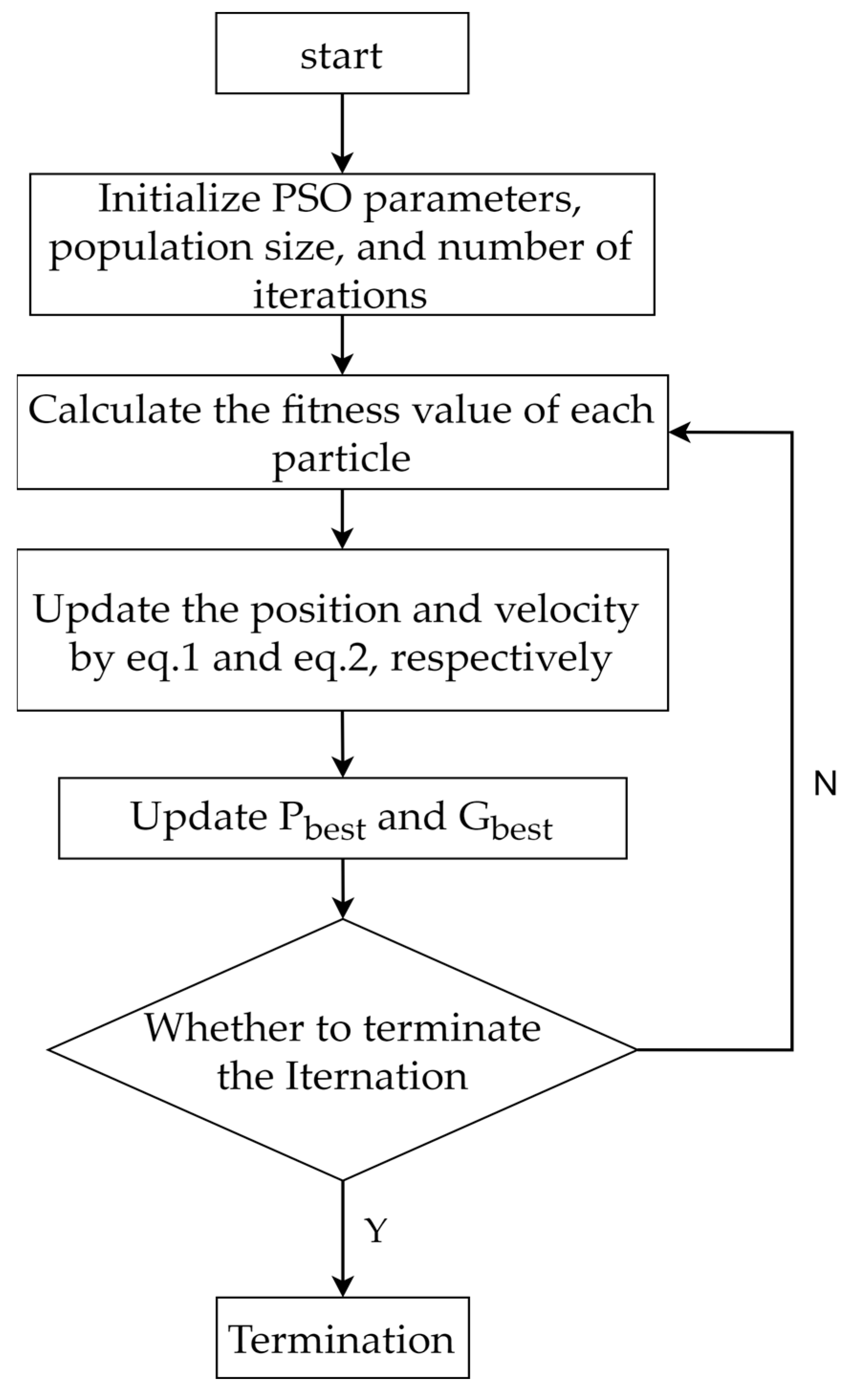
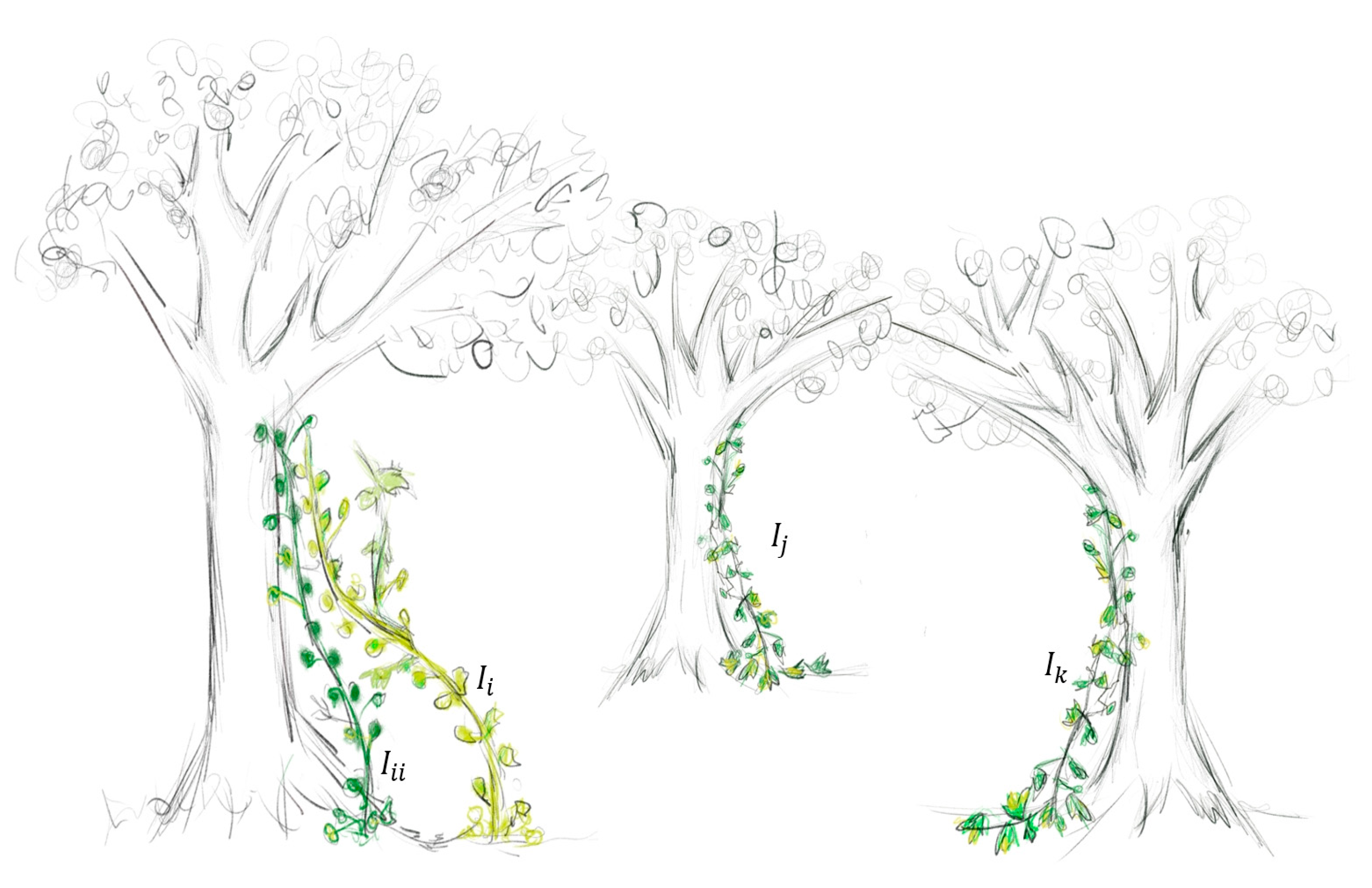


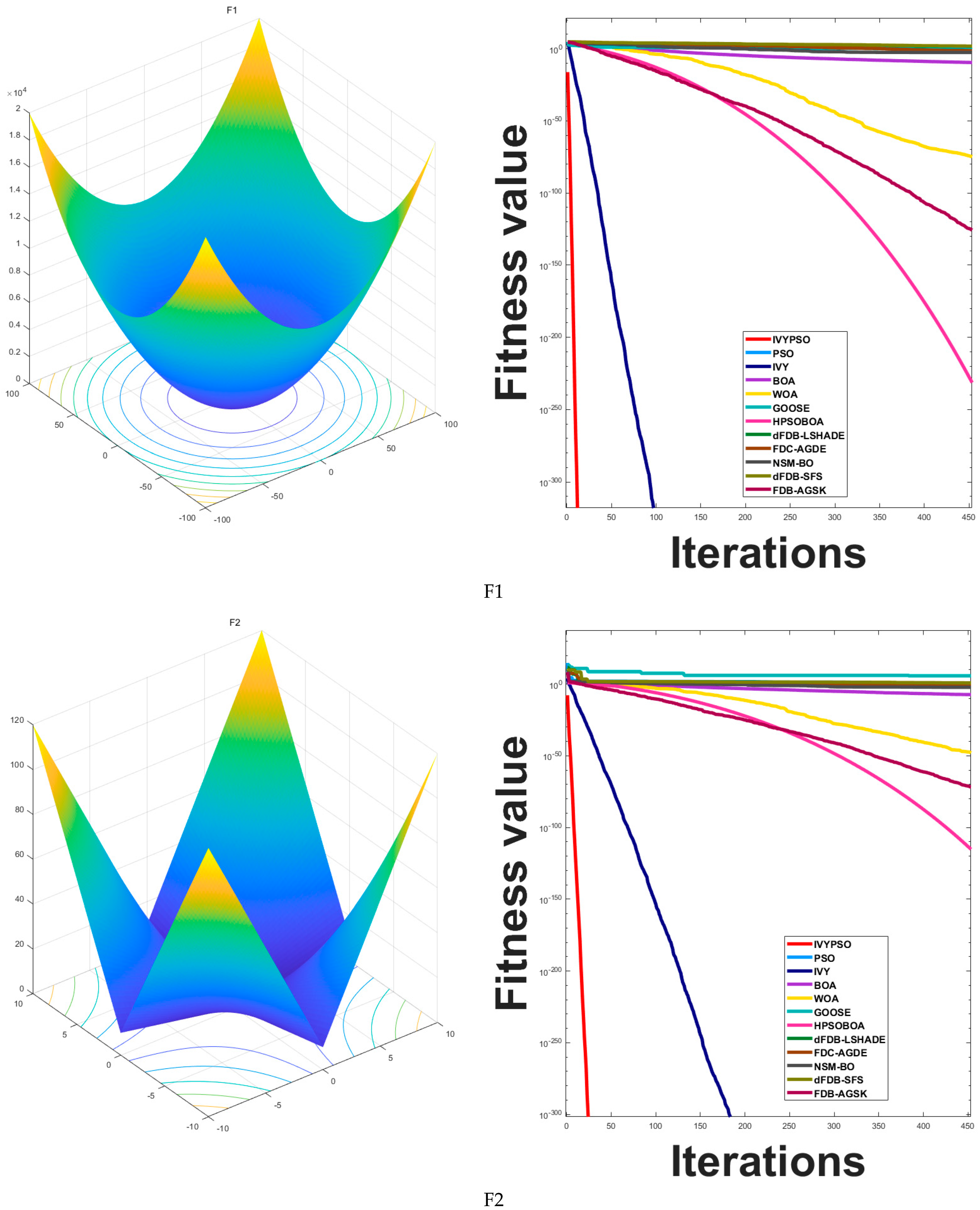


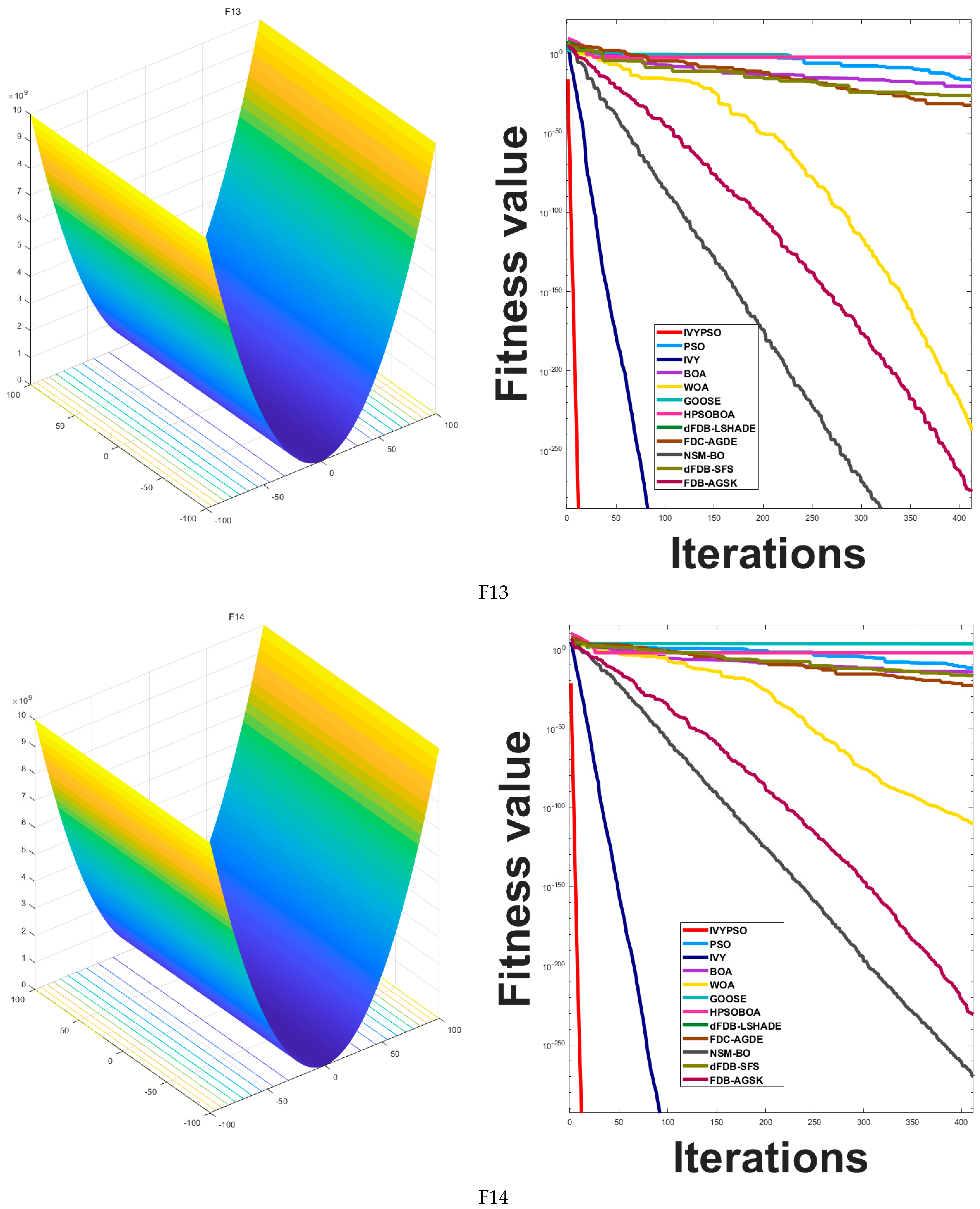
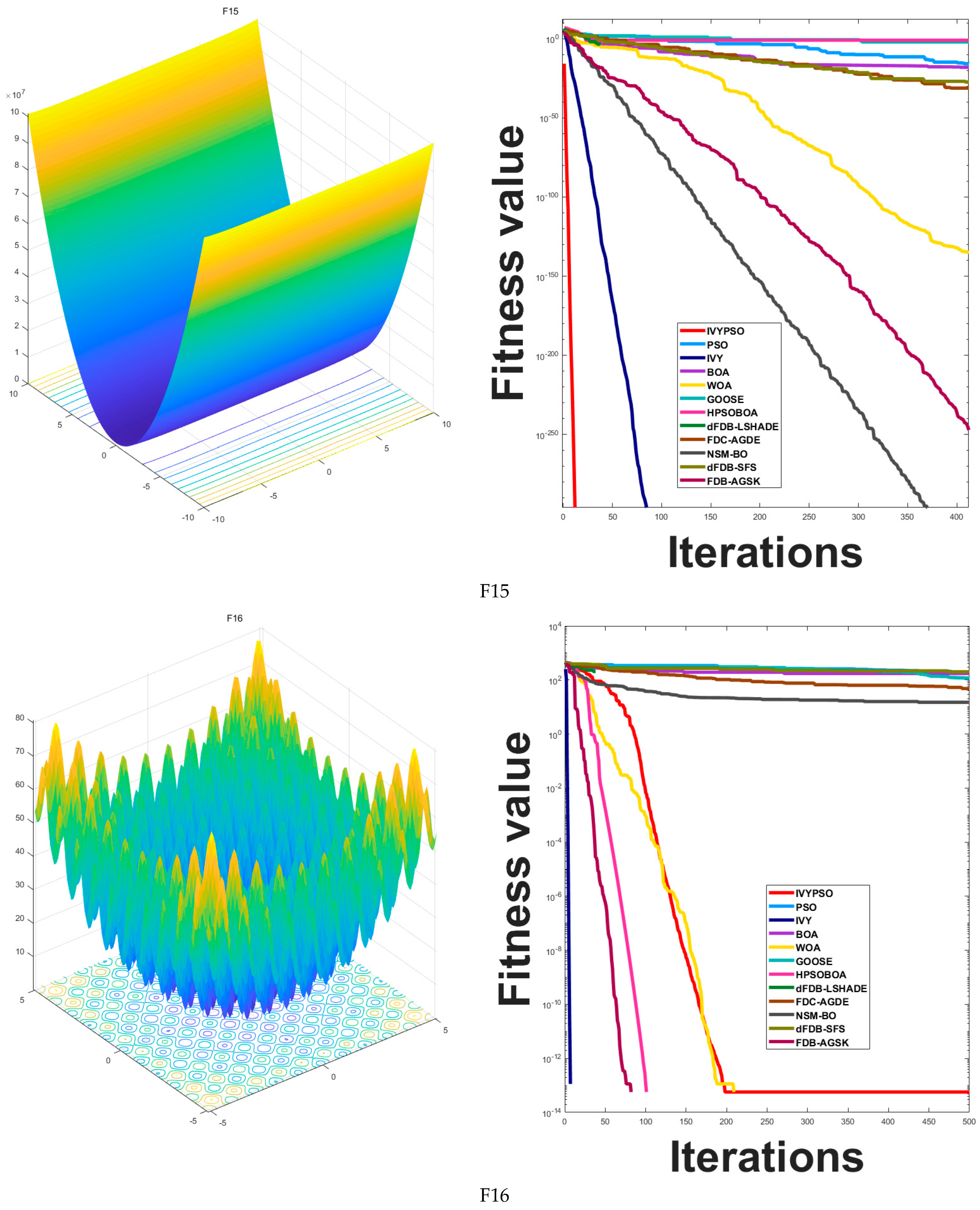
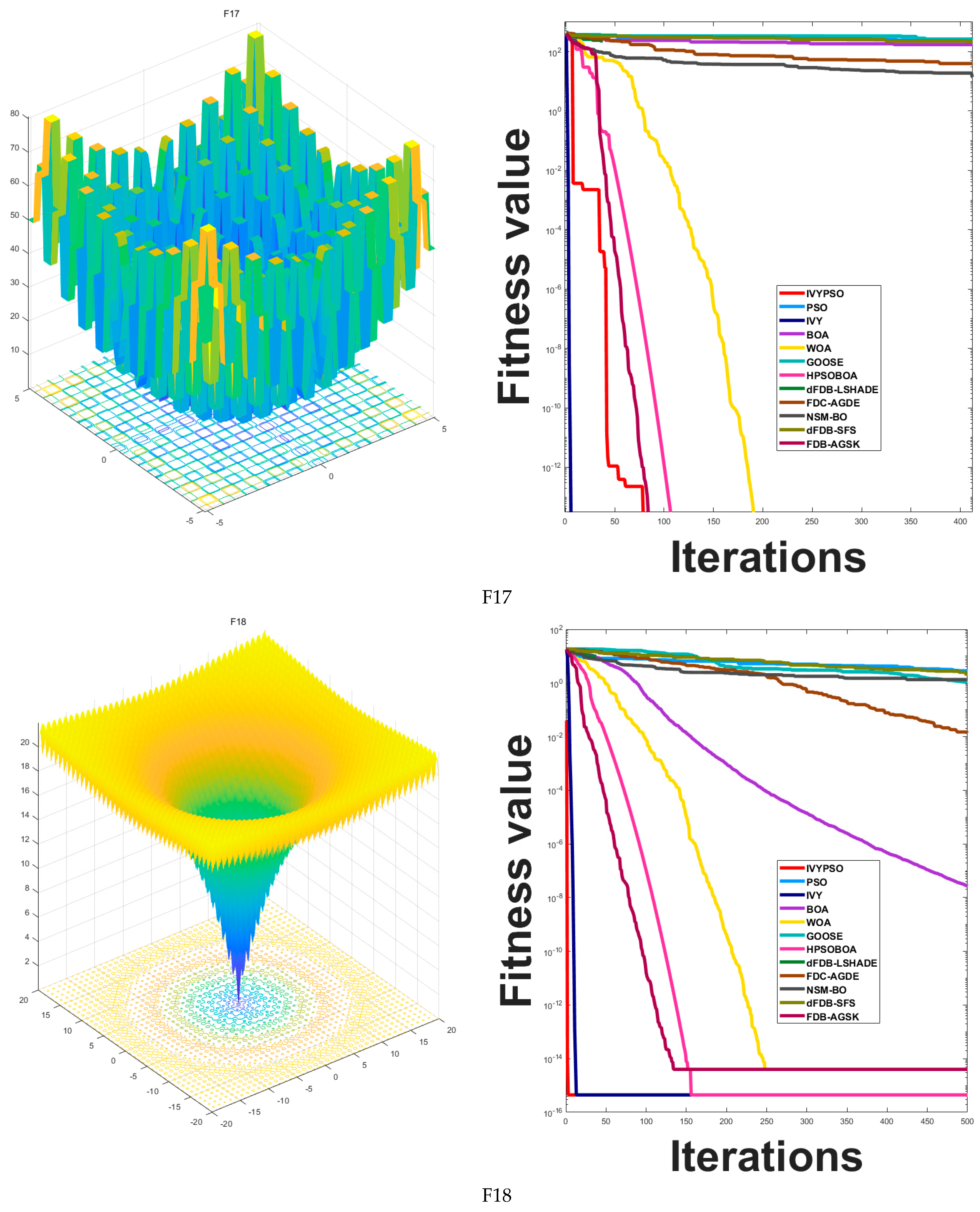


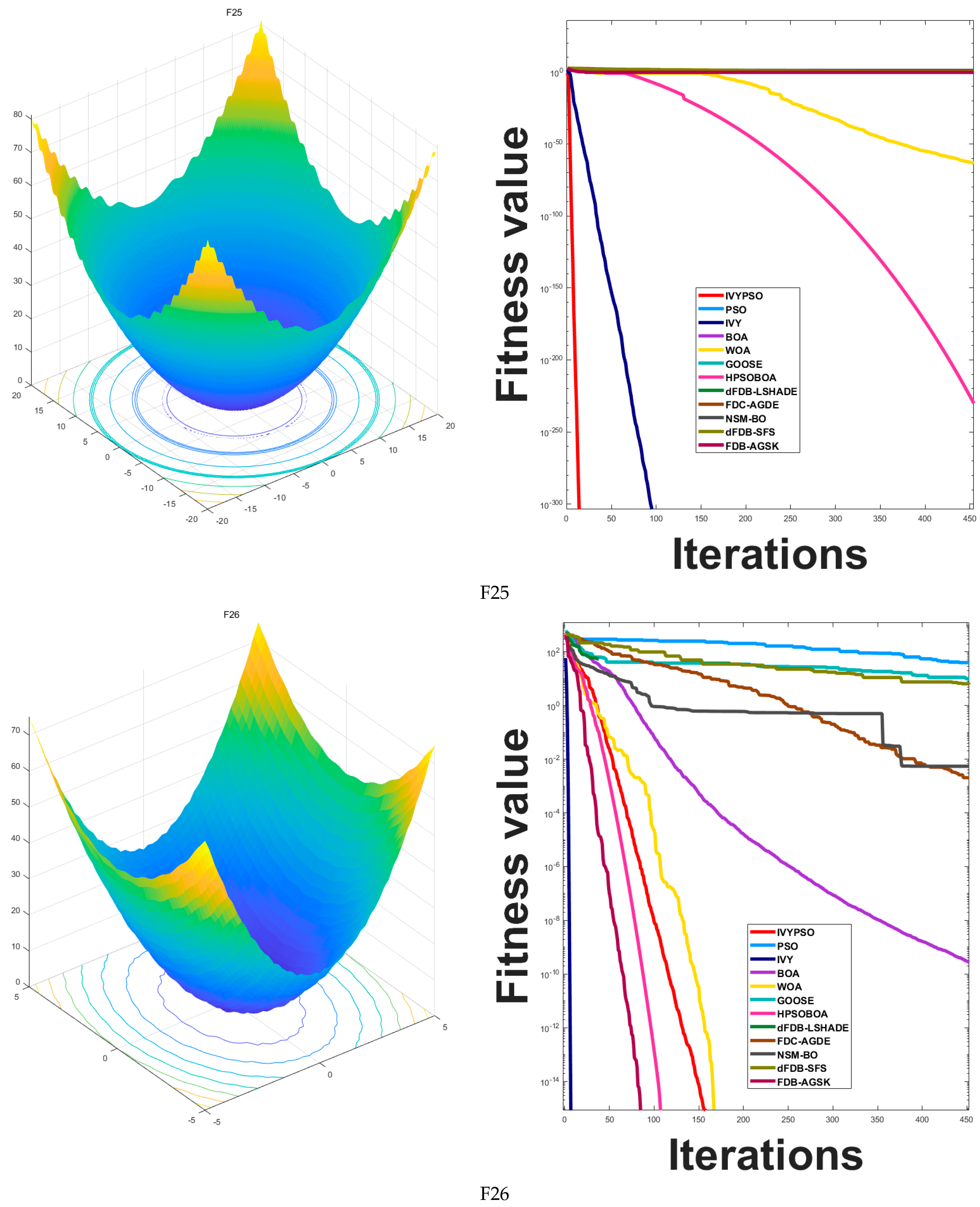
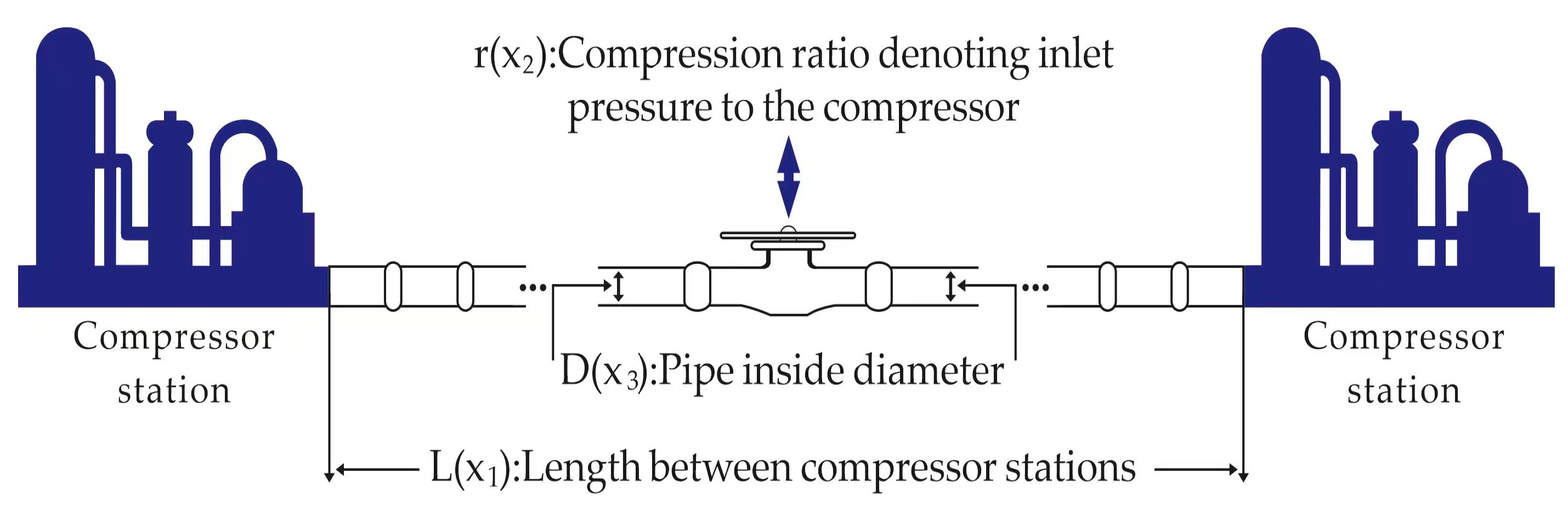


