Multi-Strategy-Assisted Hybrid Crayfish-Inspired Optimization Algorithm for Solving Real-World Problems


Abstract
1. Introduction
- They are usually inspired by some natural law or mathematical theory [35].
- No theoretical derivation is required to transform the problem into a model that is less dependent on mathematical conditions [36].
- The complexity of the algorithm determines its search rate for finding approximate and suitable solutions [37].
- (i)
- The ICOA is proposed by incorporating four strategies, namely, the elite chaotic differential strategy, differential variation strategy, Levy flight strategy, dimensional variation strategy, and adaptive parameter strategy.
- (ii)
- The effectiveness and potential of the ICOA in addressing complex optimization problems are validated through experimental results obtained from benchmark test sets such as CEC2017, CEC2019, and CEC2020. These results are compared with other state-of-the-art swarm intelligence optimization algorithms, revealing the superior performance of the ICOA. This comparative analysis highlights the algorithm’s effectiveness and reinforces its capability to tackle challenging optimization problems.
- (iii)
- The ICOA is applied to various real-world industrial design problems, including six specific cases. In addition, thirty high–low-dimension constraint problems, two NP problems, and one hypersonic missile trajectory planning problem are evaluated. The performance of the ICOA is methodically compared to that of classical or state-of-the-art optimization algorithms, providing insights into its efficacy and applicability across diverse problem domains.
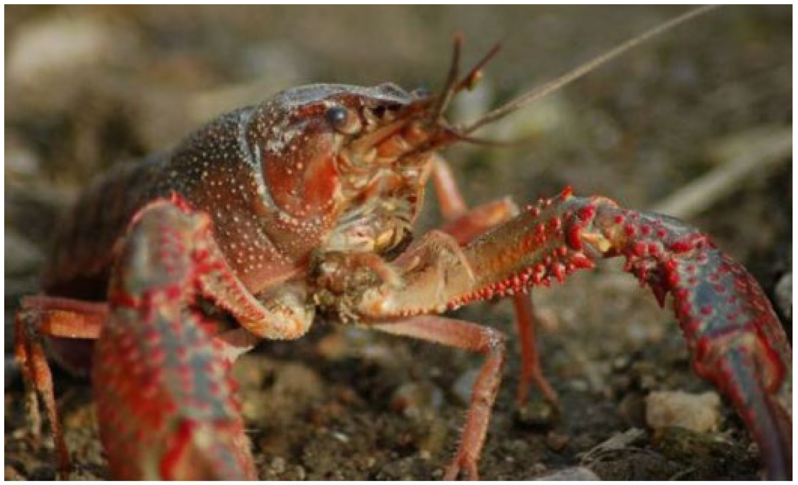
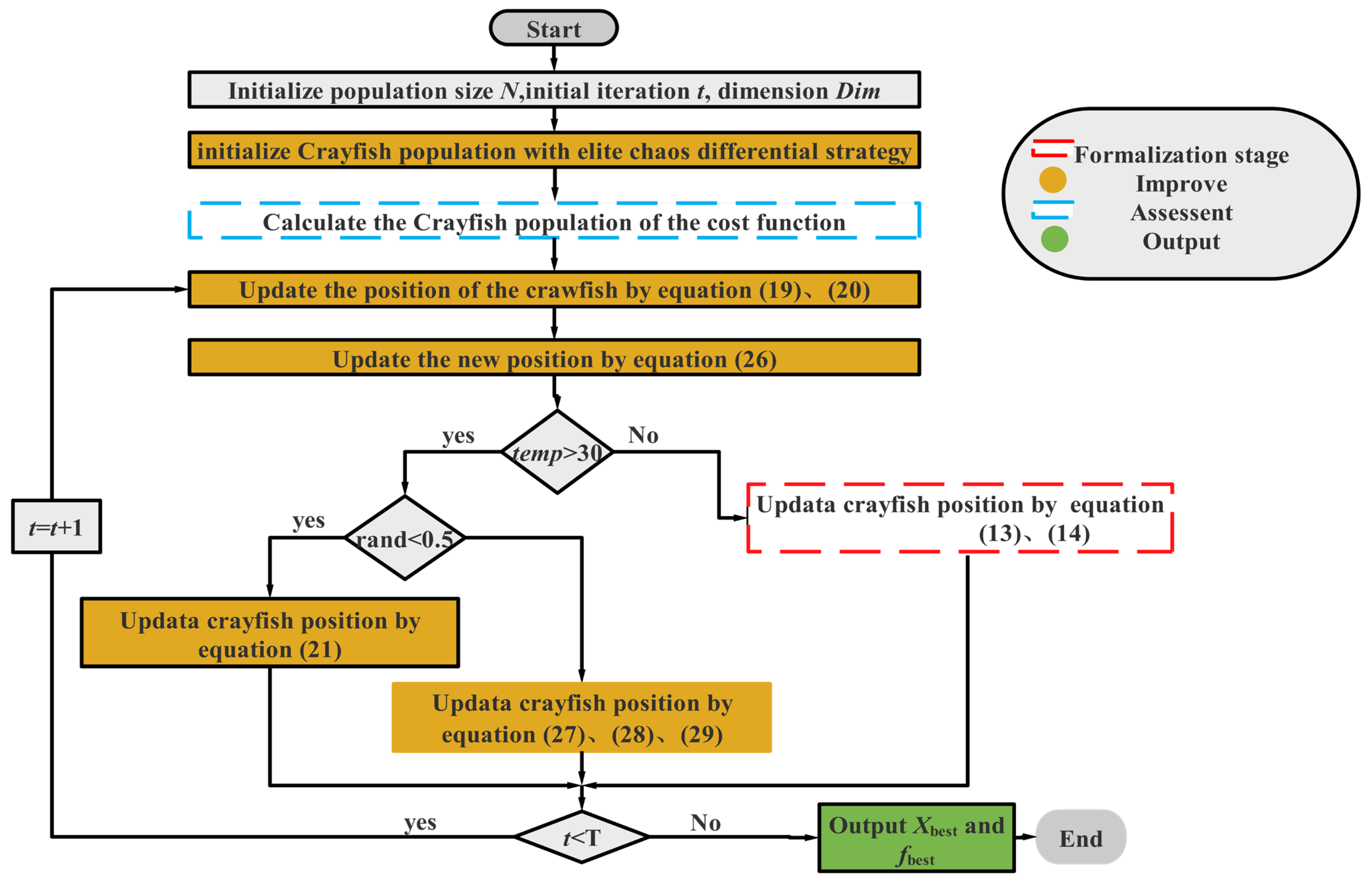
2. Overview of the Crawfish Optimization Algorithm
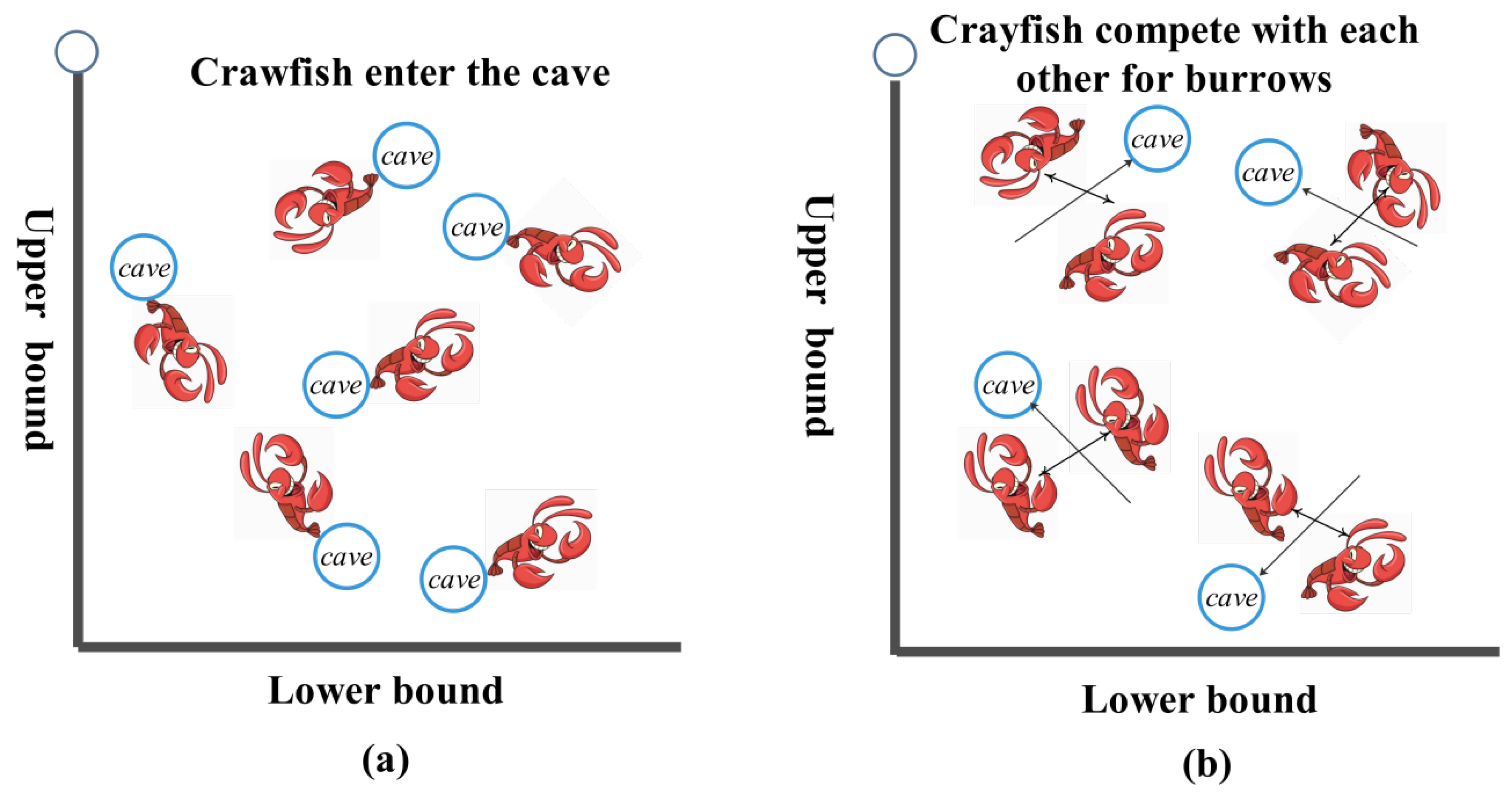
2.1. Summer Vacation
2.2. Competition Stage
2.3. Formalization Stage
| Algorithm 1: Crayfish optimization algorithm |
| Begin Step 1: Initialization. Set the parameters of the crayfish population. |
| Step 2: Fitness calculation. By calculating the fitness value of the initialized population to get . |
| Step 3: while termination criteria are not met do |
| Defining temperature temp by Equation (3) |
| if temp > 30 do |
| Define cave according by Equation (5) |
| if rand < 0.5 do |
| Crayfish conducts the summer resort stage according to equation (6) |
| else |
| Crayfish compete for caves through Equation (8) |
| end |
| else |
| P and Q can be found by Equation (4) and Equation (11), respectively. |
| if Q ≥ 2 do |
| Crayfish shreds food by Equation (12) |
| Crayfish foraging according to Equation (13) |
| else |
| Crayfish foraging according to Equation (14) |
| end |
| end |
| Update fitness value and output . |
| end while |
3. Improved Crayfish Optimization Algorithm with Mixed Strategies
3.1. Elite Chaos Difference Strategies
- (1)
- Elite learning selects the population according to a certain ratio as the first part of the initialization decomposition.
- (2)
- Logistic chaotic mapping is carried out on the remaining population according to the ratio column as the second part of the initialization solution.
- (3)
- Differential learning, which is performed on the remaining populations, randomizes the elite populations as well as the chaotically mapped populations to be updated by the differential operation to obtain the final differential population, which is the last part of the initial solution.
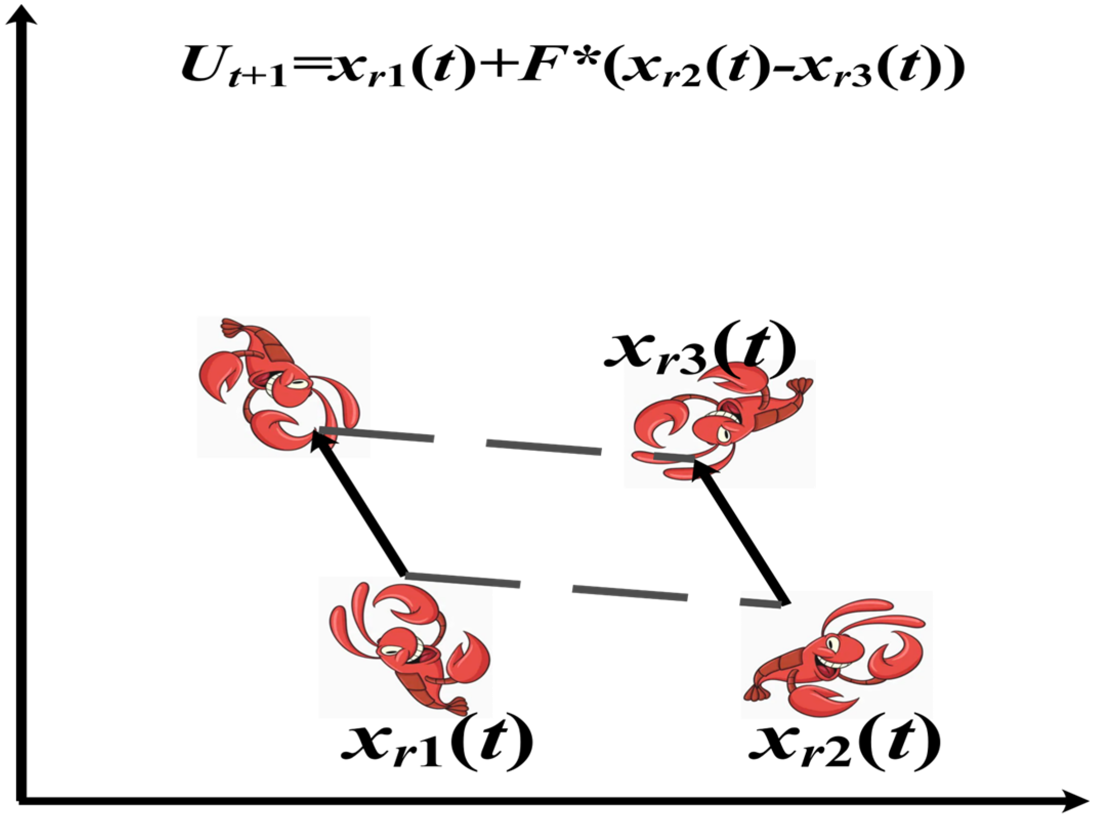
3.2. Differential Variation Strategy
- (1)
- Mutation operation
- (2)
- Selection operation
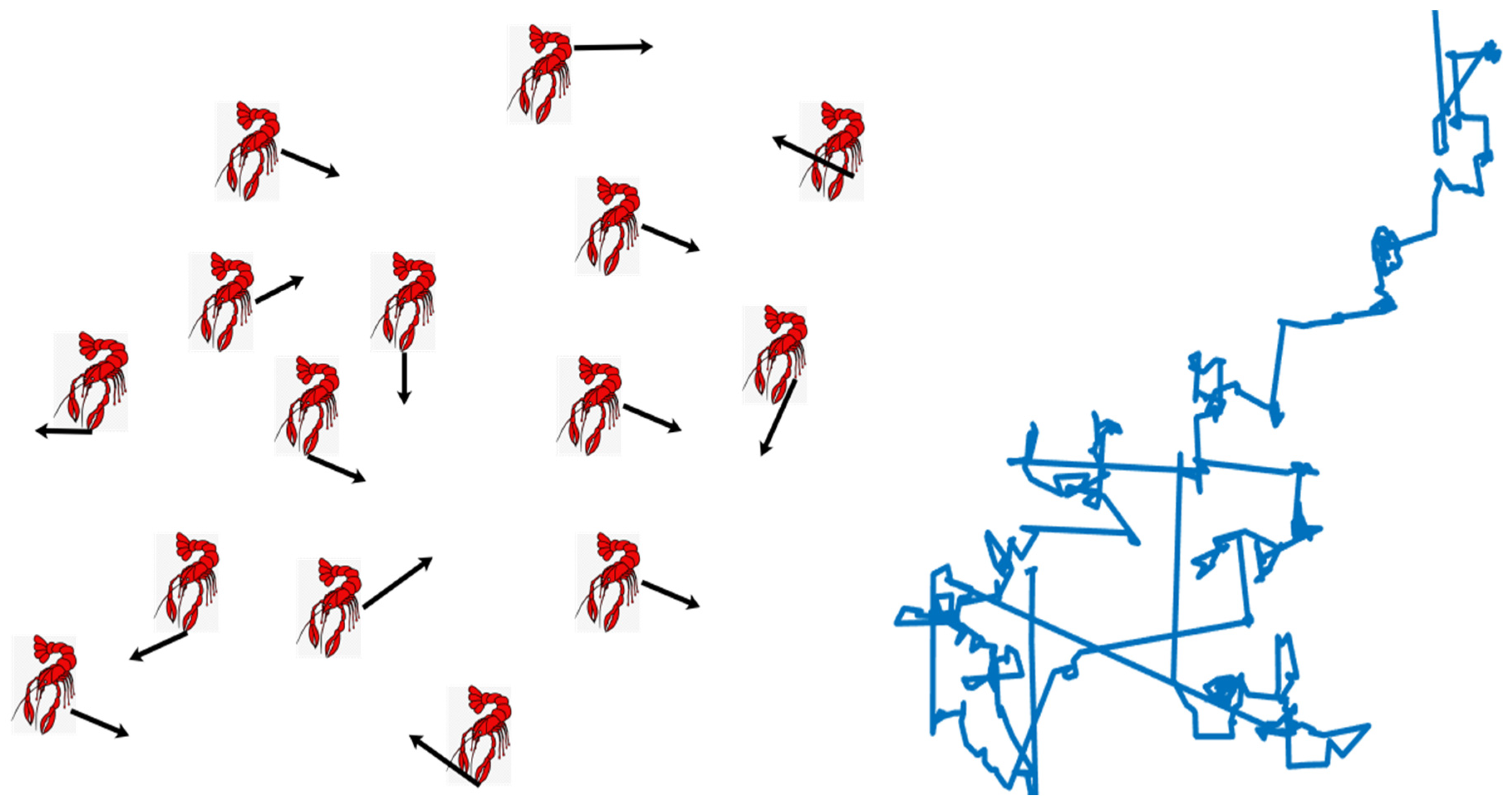
3.3. Levy Flight Strategy
3.4. Dimensional Variation and Adaptive Parameter Strategy
3.4.1. Dimensional Variation Strategy
3.4.2. Adaptive Parameter Strategy
3.5. ICOA Pseudo-Code
| Algorithm 2: The proposed ICOA |
| Begin Step1: Initialization. Crayfish populations were initialized using the elite chaos differential strategy (i.e., Equation (18)). Step2: Fitness calculation. By calculating the population fitness value fitness, the optimal fitness value as well as the corresponding individuals were recorded; Step3: While (t < T) do Defining temperature temp by Equation (3) for i = 1 to N do //Mutation operation //Select operation end for //Dimensional variation for i = 1 to N do if temp > 30 do //Summer resort stage and competition stage if rand < 0.5 do Else //Competition stage For j = 1 to Dim do end for end else //forging stage if P >2 do else end end for Calculate and rank the fitness values. Update t = t+1 Step4: Return. Return the optimum position and fitness value of Crayfish End |
3.6. Time Complexity of the ICOA
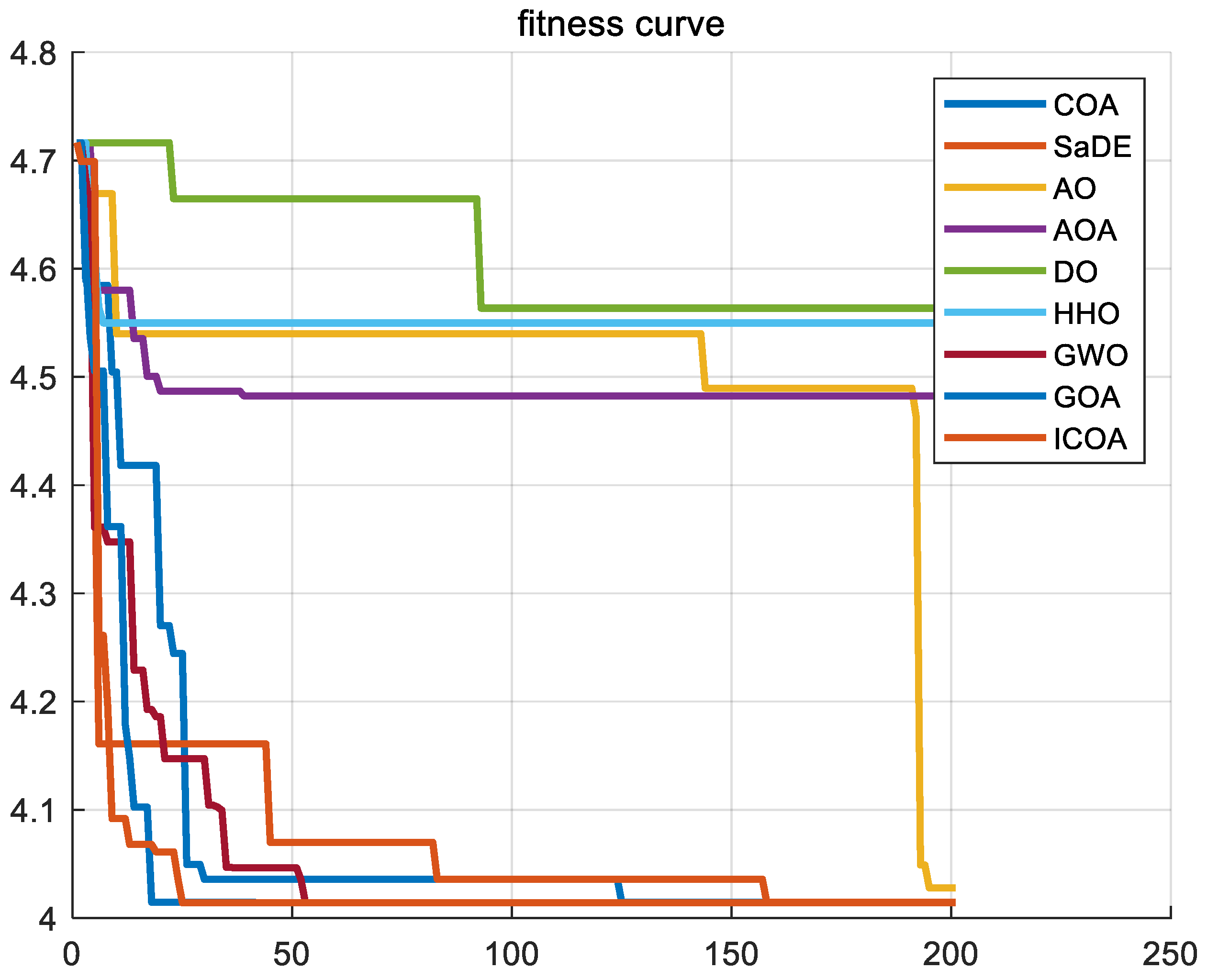
4. Numerical Experiment and Analysis
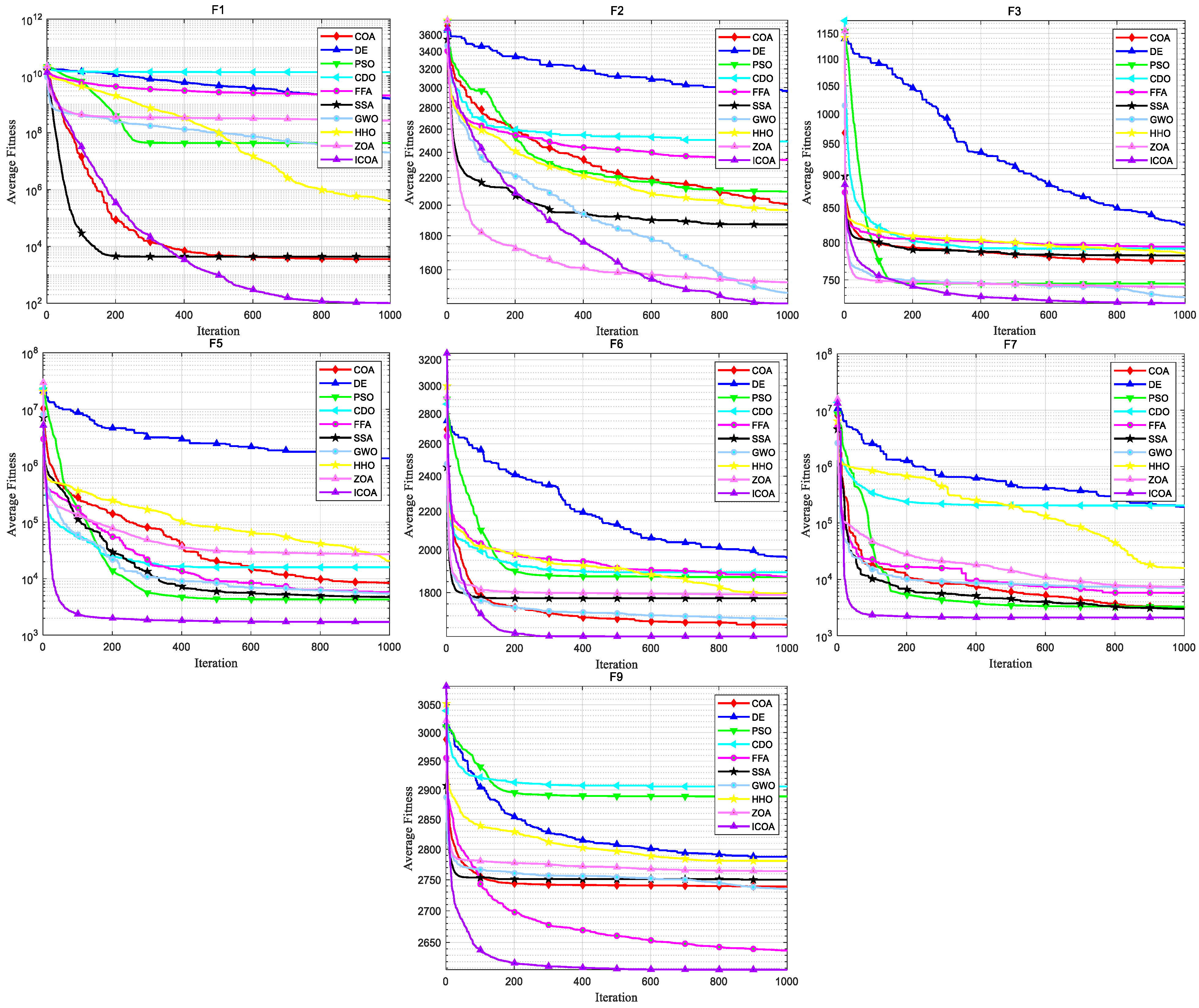
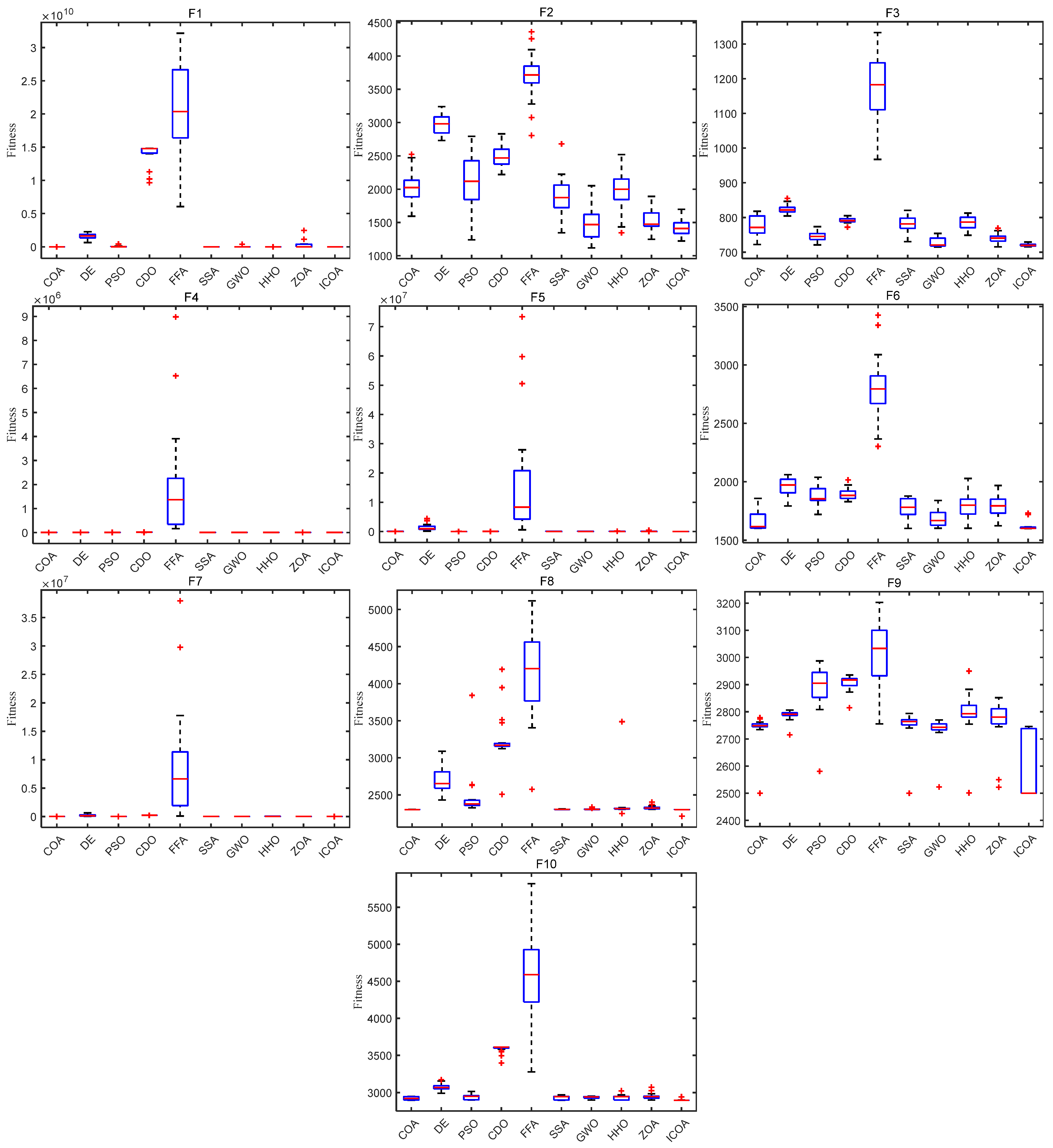
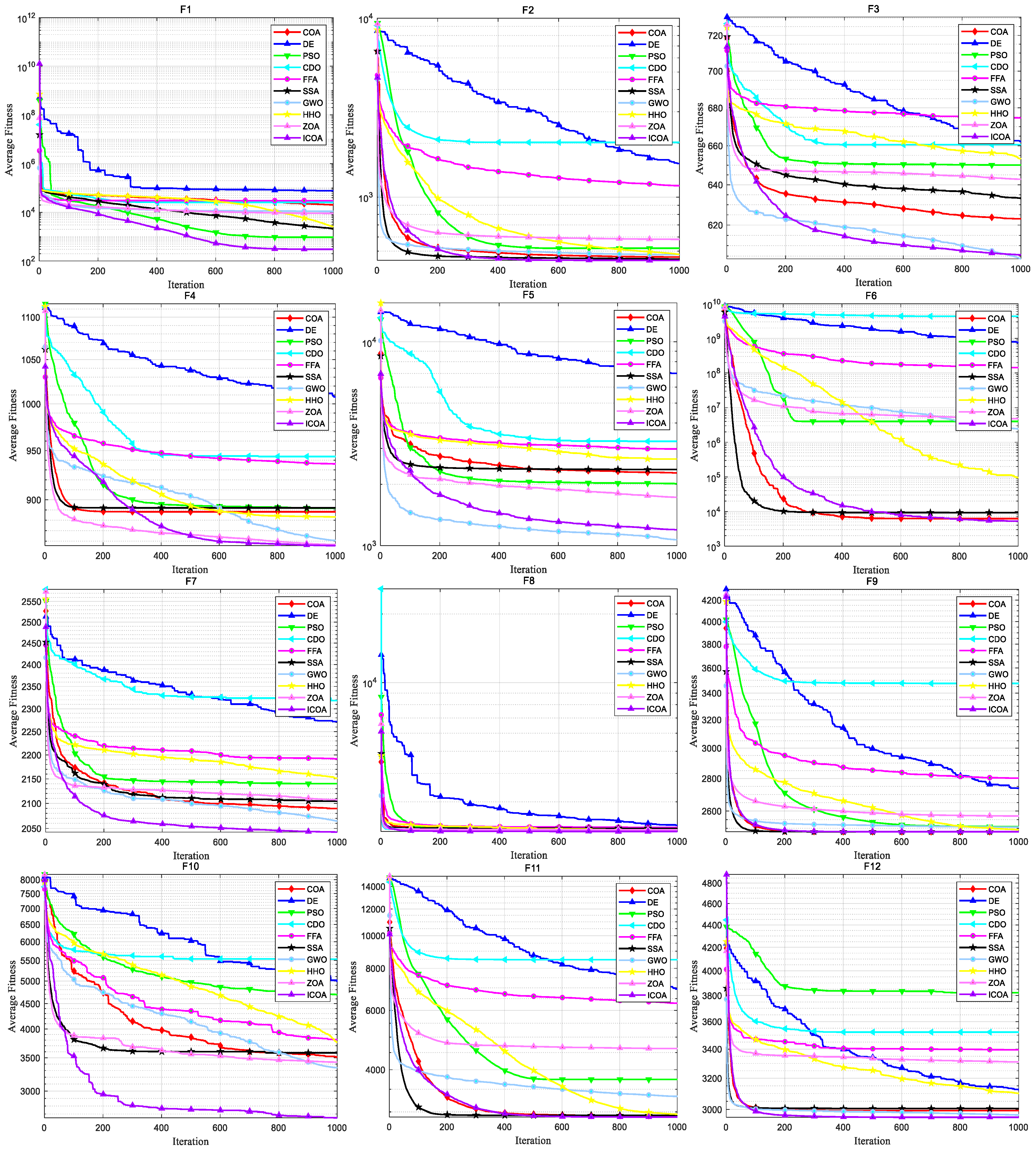
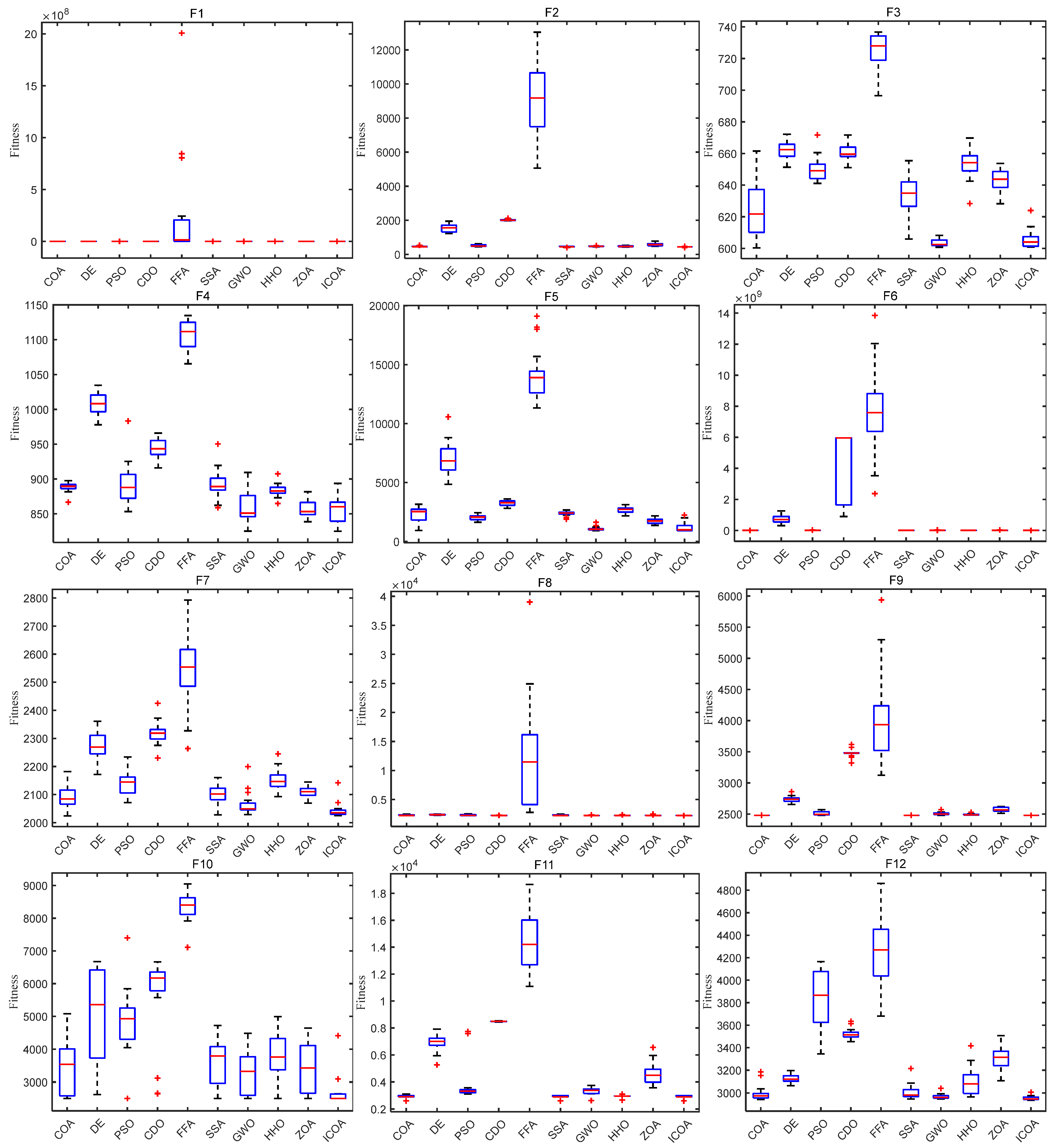
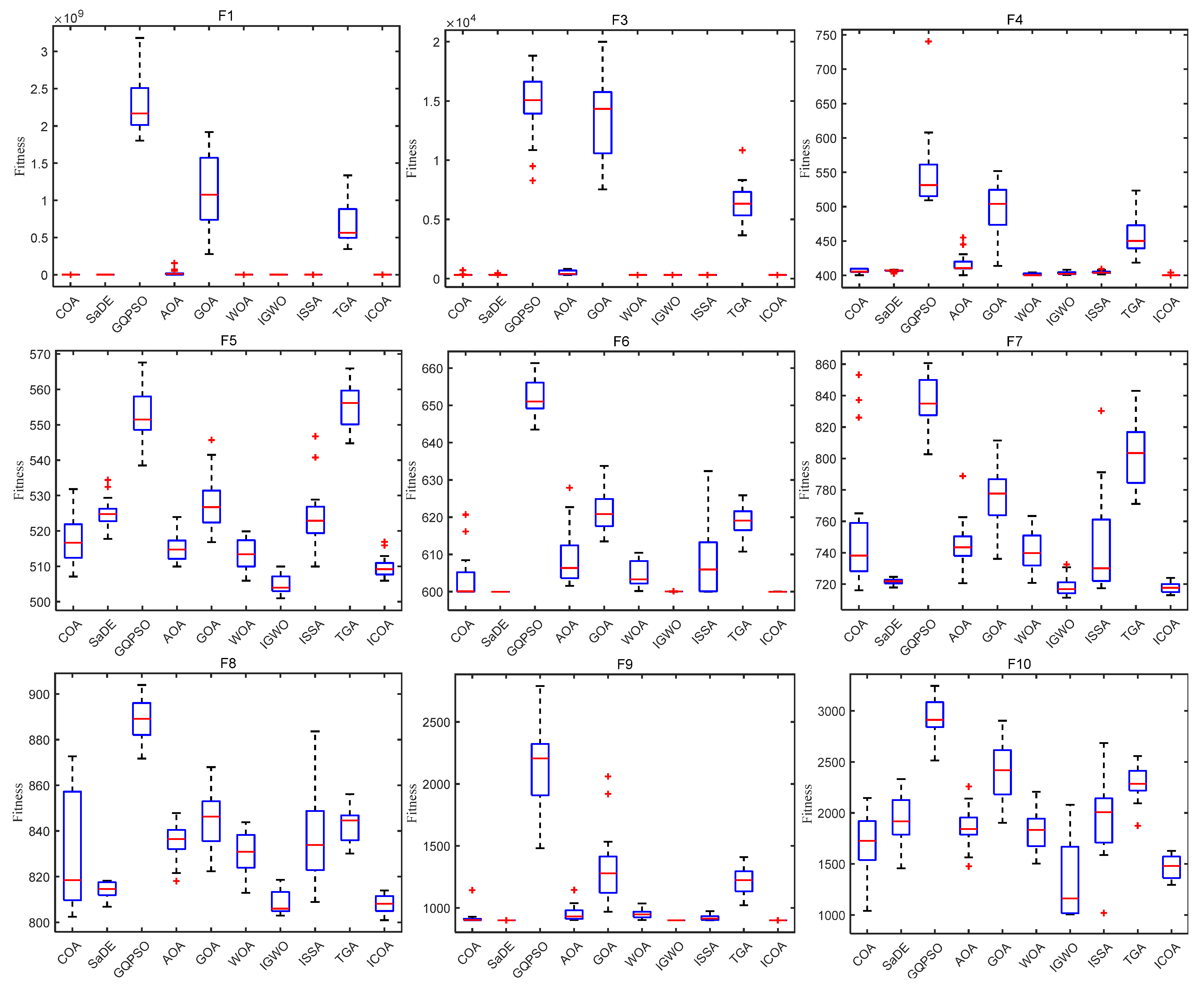
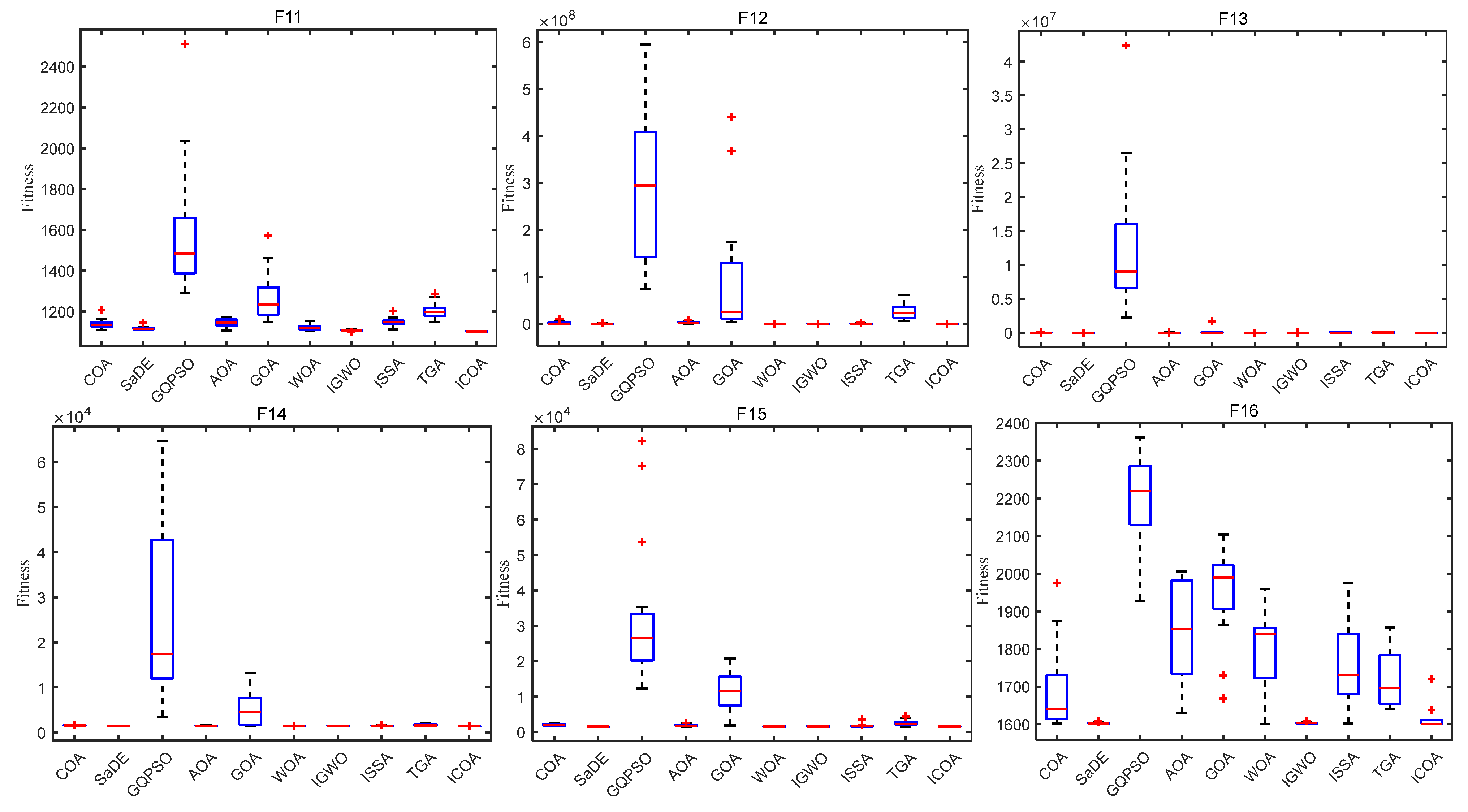
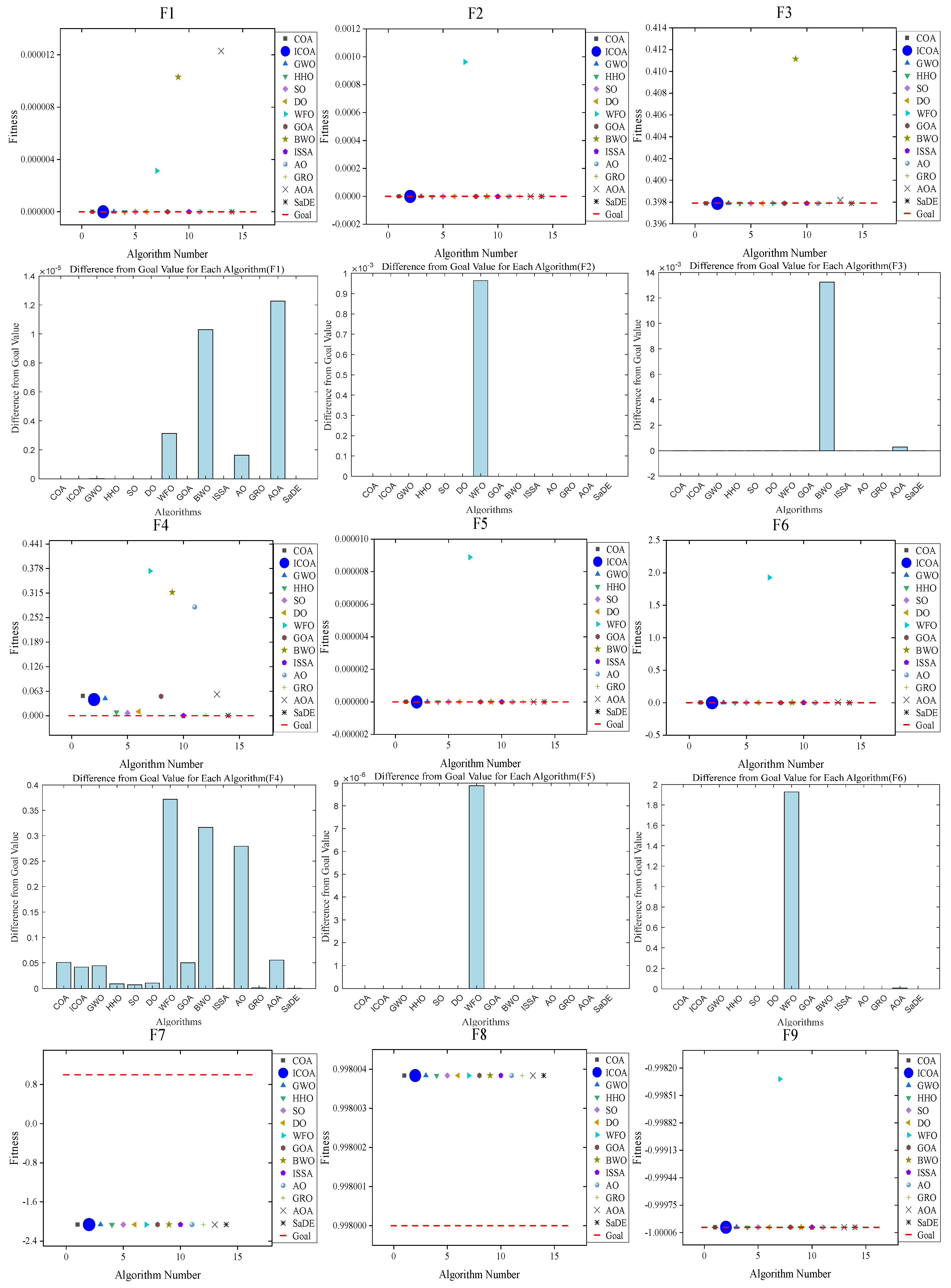
4.1. ICOA Is Compared with the First Group of Optimization Algorithms
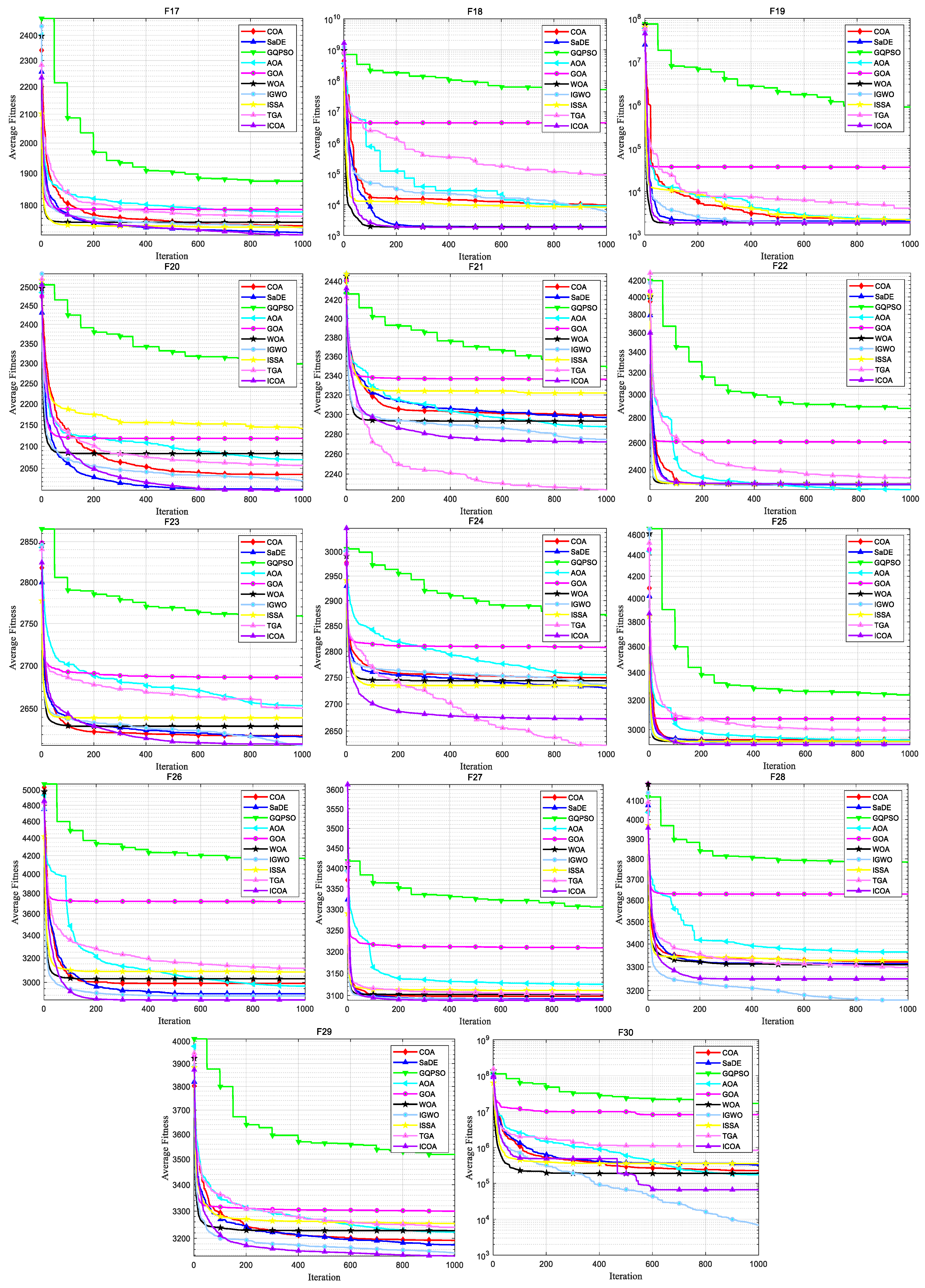
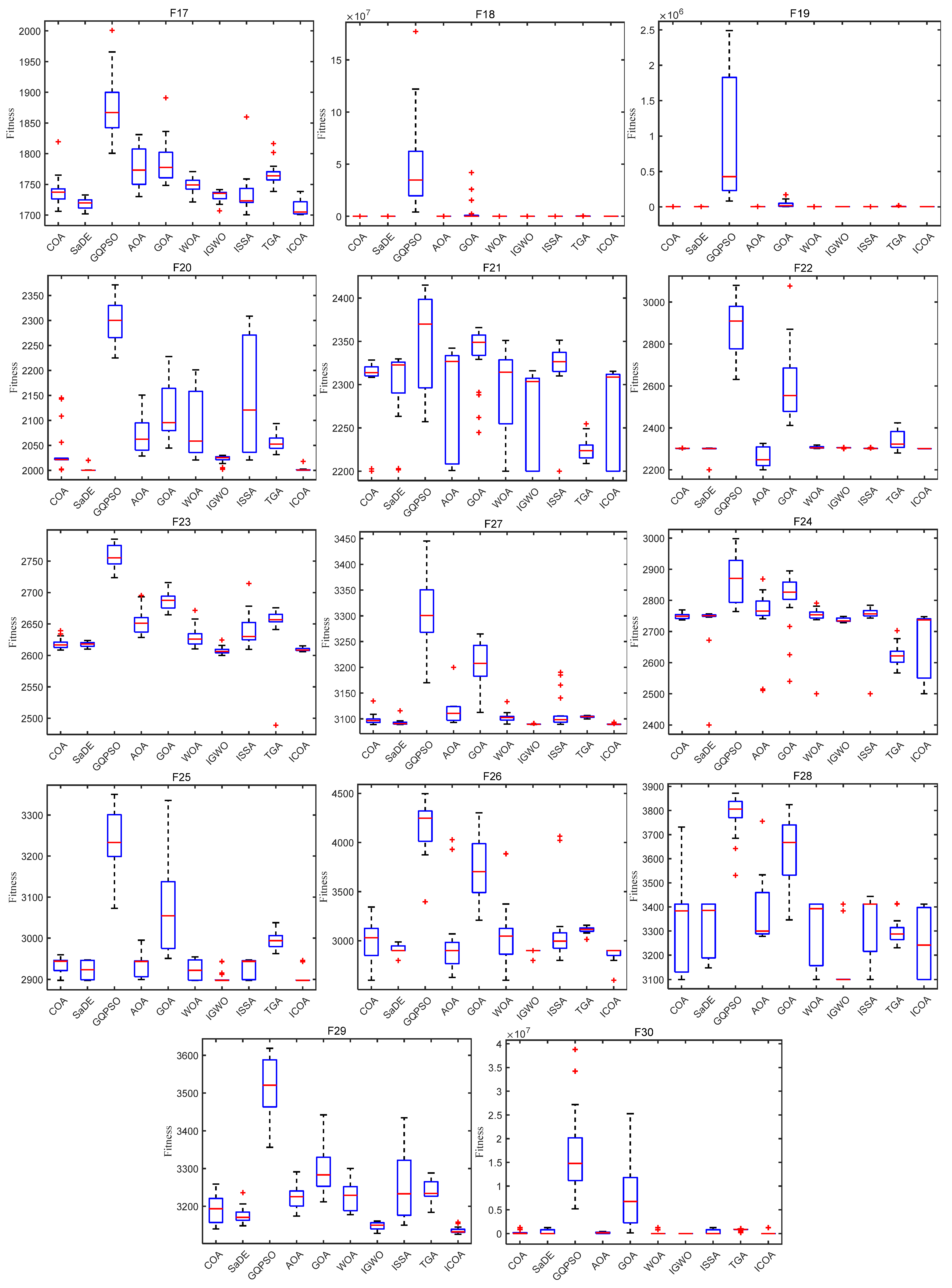
4.1.1. Comparison of the Test Set CEC 2020
4.1.2. Comparison on Test Set CEC 2022
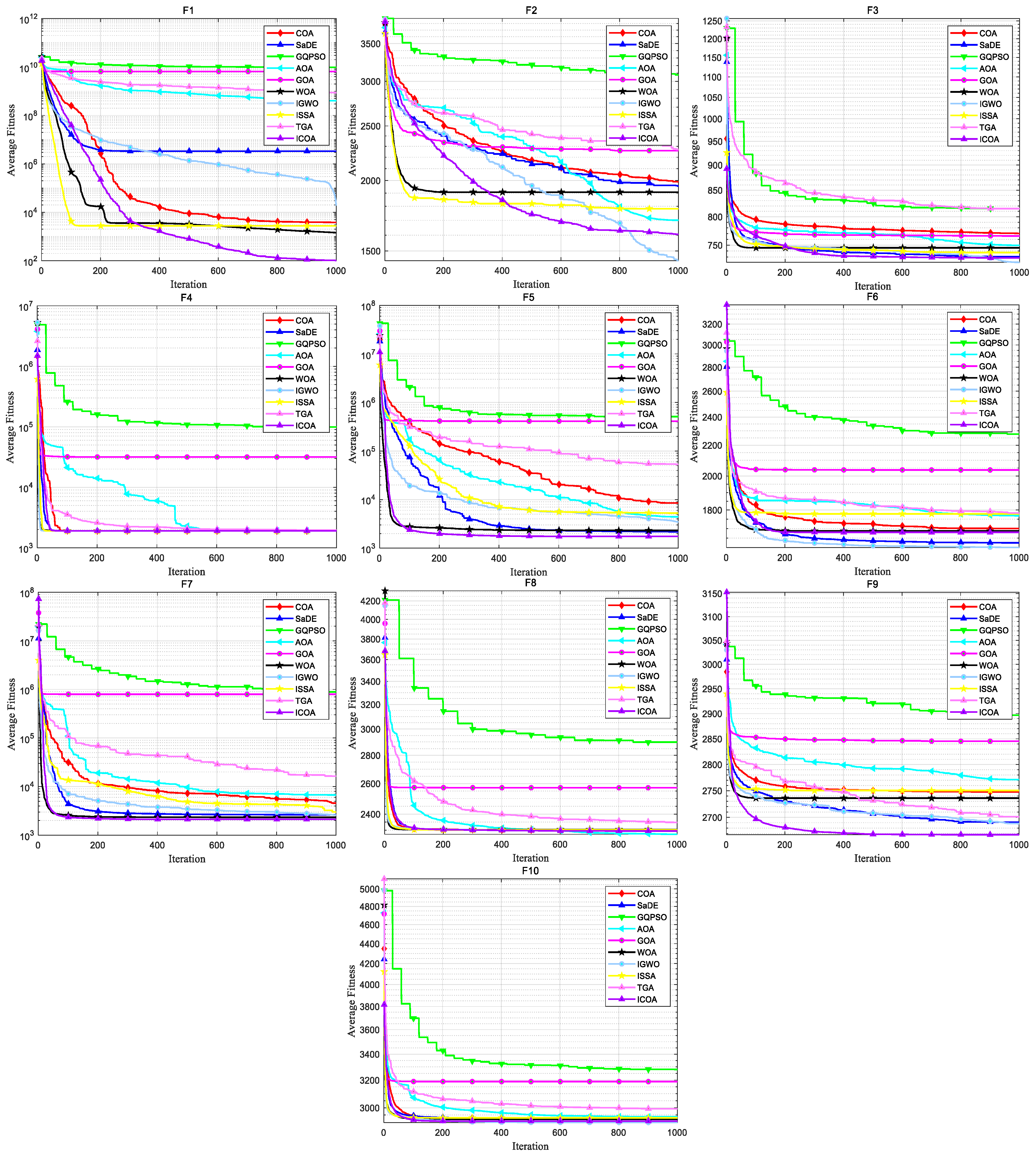
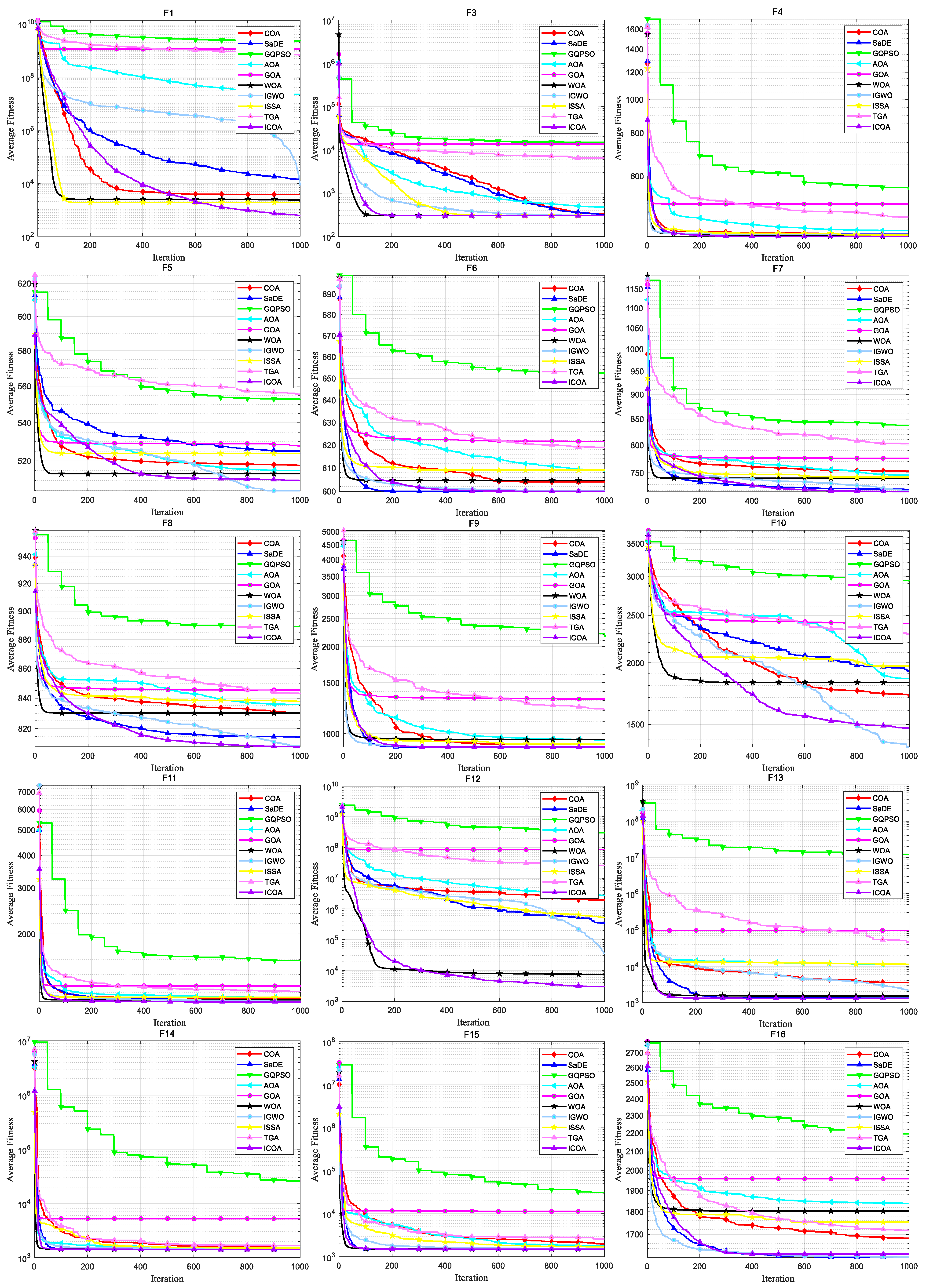
4.2. ICOA Compared with the Second Group of Optimization Algorithms
4.2.1. Comparison on CEC 2020 Test Set
4.2.2. Comparison on Test Set CEC 2017
5. ICOA Solves All Kinds of Optimization Problems
5.1. ICOA Solves Engineering Optimization Problems
5.1.1. Speed Reducer Design Problem
5.1.2. Hydrodynamic Thrust Bearing Design Problems
5.1.3. Welded Beam Design Problem
5.1.4. Robot Gripper Design Optimization Problem
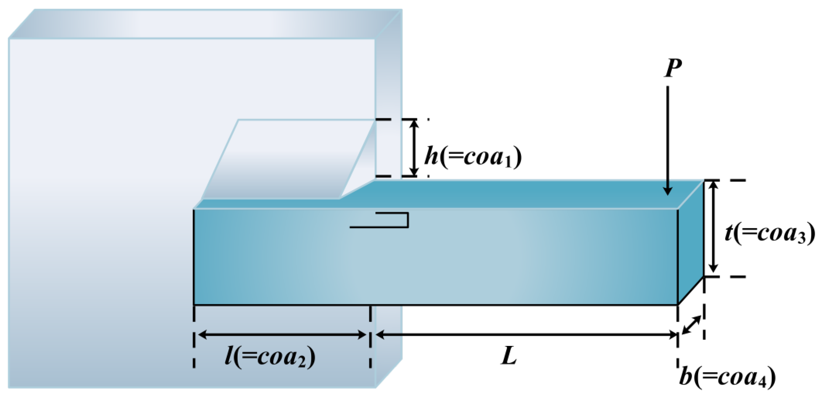
5.1.5. Cantilever Beam Design Issues
5.1.6. Heat Exchanger Design Issues
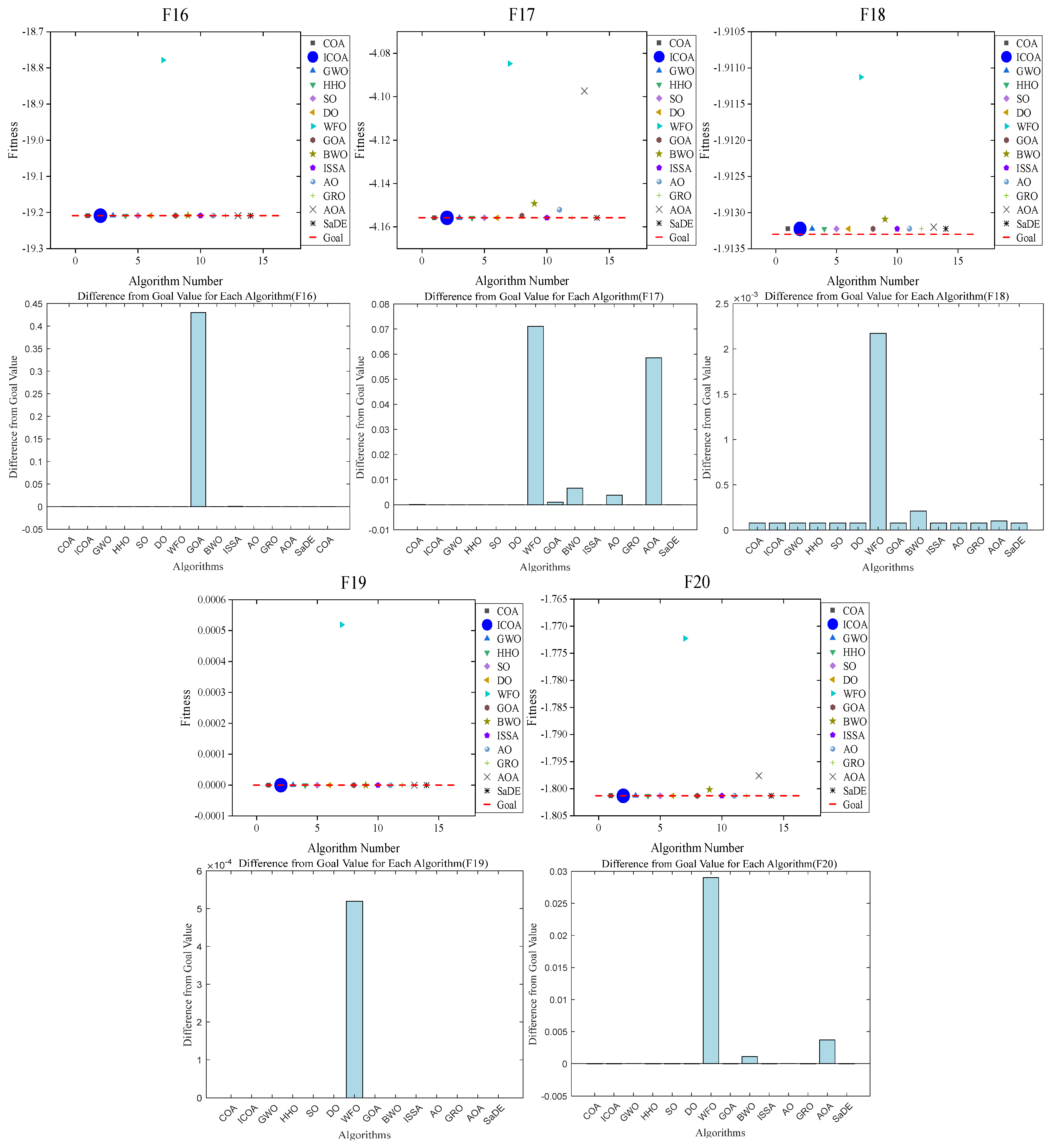
5.2. ICOA Solves Constrained Optimization Problems
5.2.1. Low-Dimensional Problems
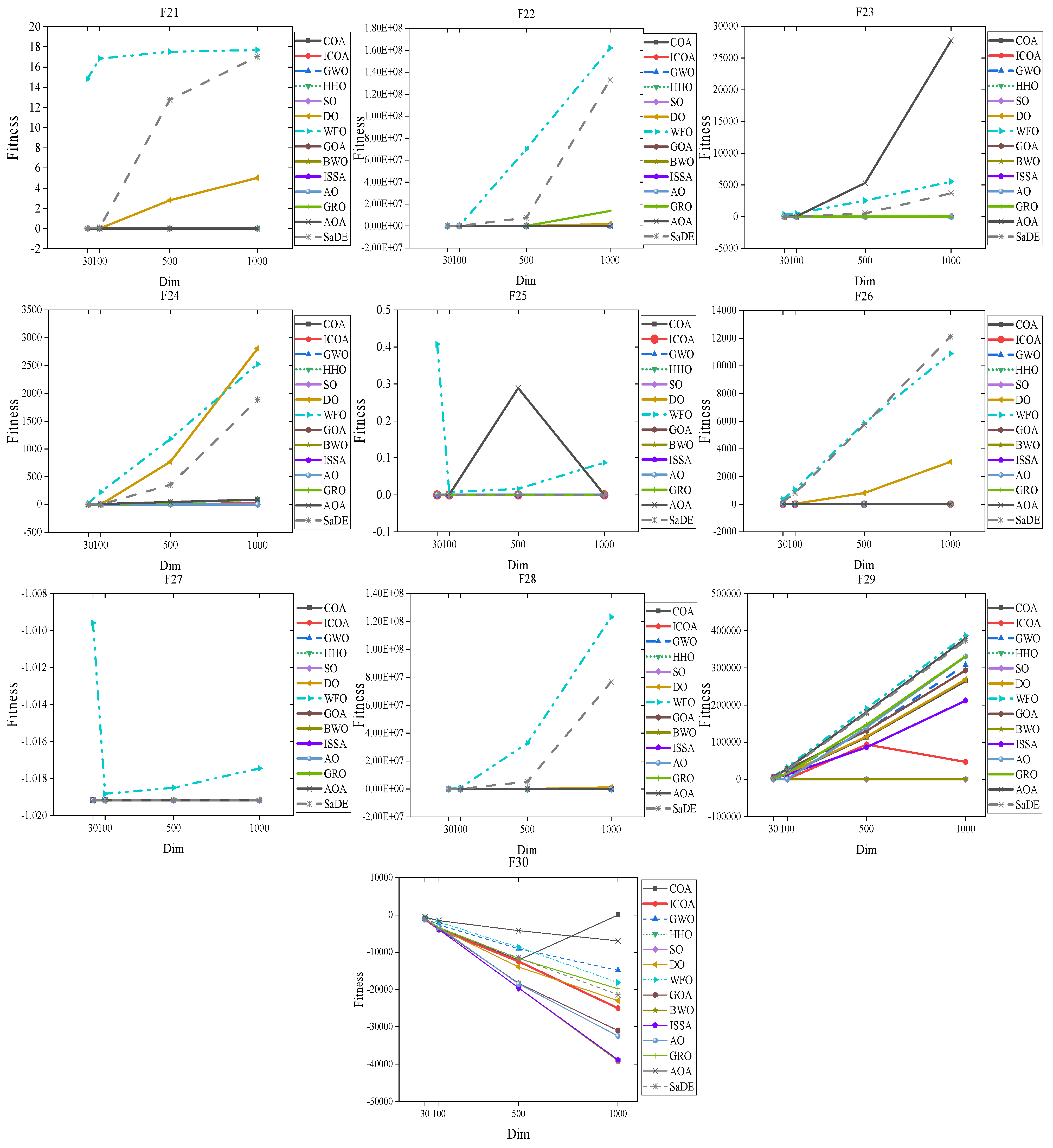
5.2.2. Higher Dimensional Problems
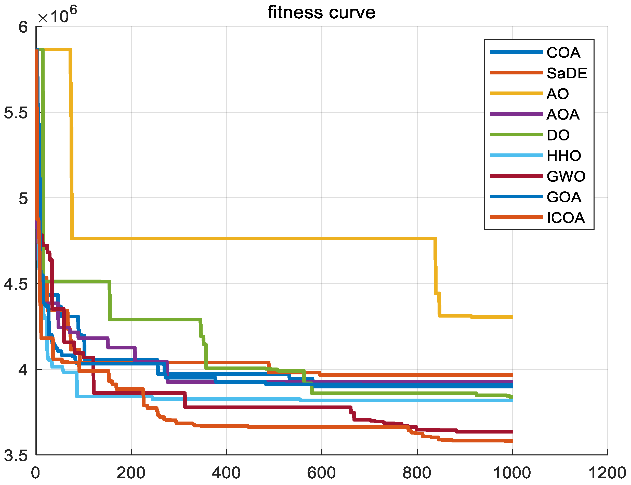
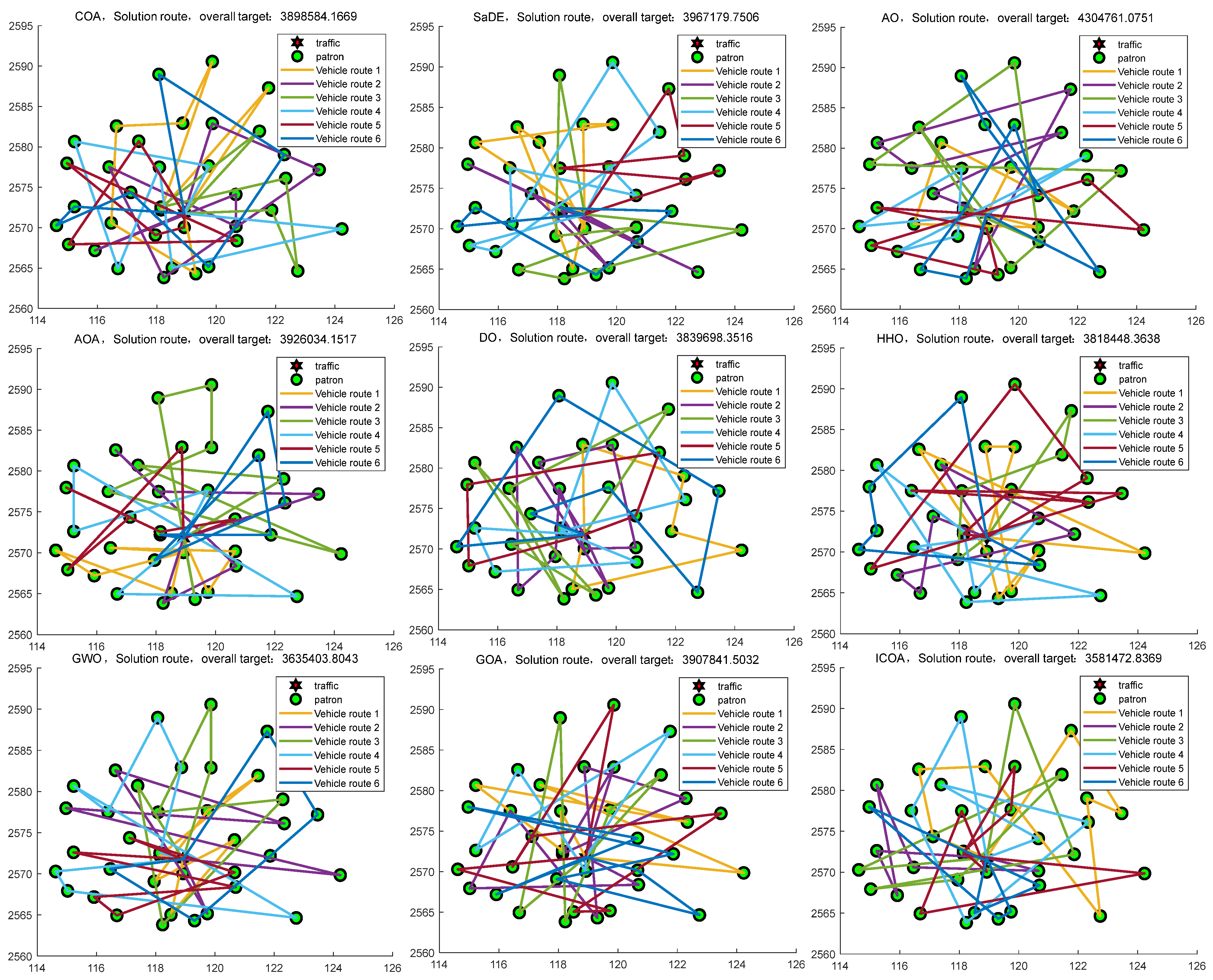
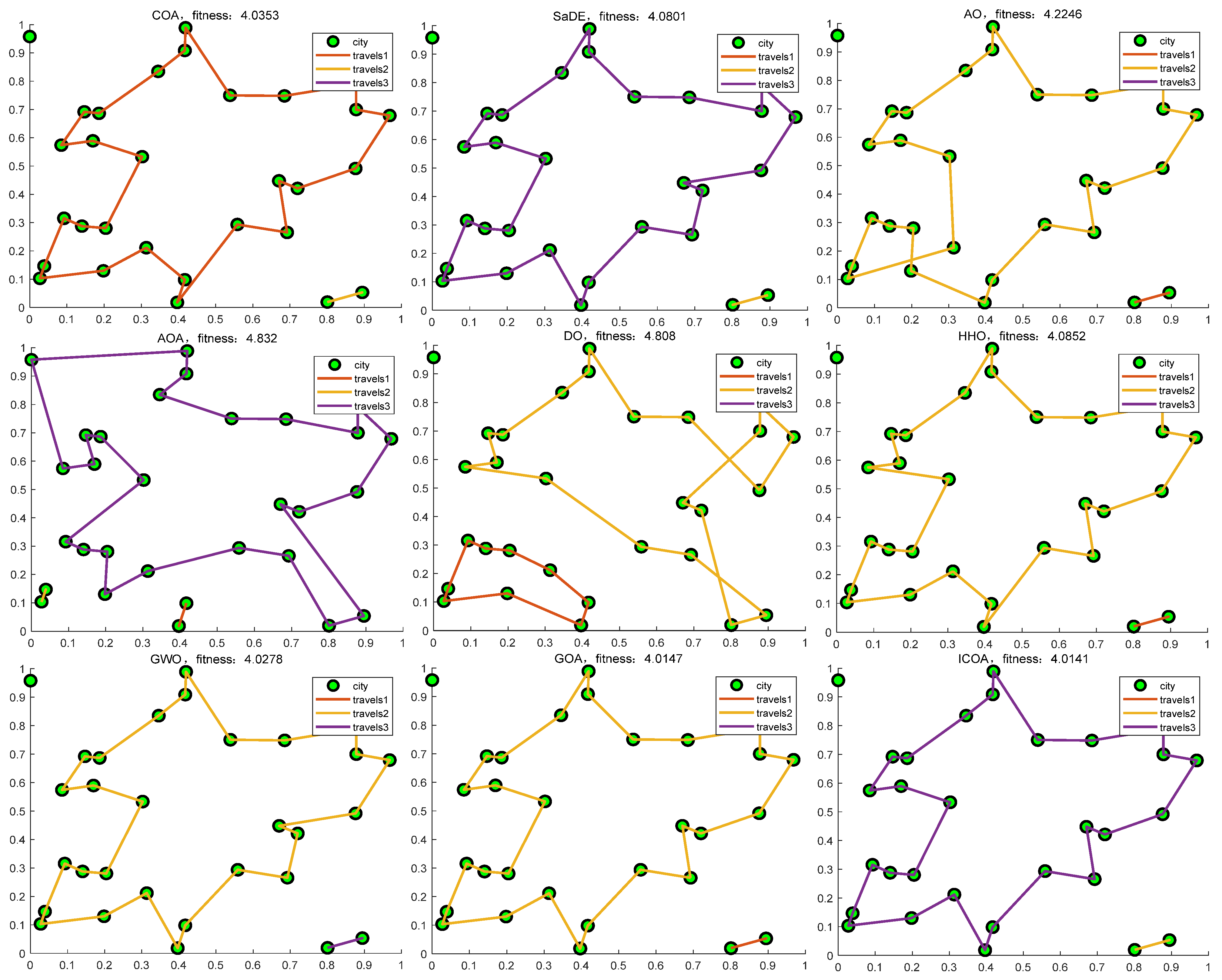
5.3. ICOA Solving the NP-Hard Problem
- A.
- NP1. logistics distribution [75]
- B.
- NP2. TSP issues [75]
6. Discussion
7. Conclusions and Future Work
- (1)
- The elite chaotic difference strategy improves good initial solutions for the ICOA, prevents blind searches, and ensures a more uniform distribution of populations in space.
- (2)
- The ICOA ranks first in all the CEC 2020 test sets, and tenth out of twelve test functions in the CEC 2022 test set, based on the first set of comparison algorithms. Based on the second set of comparison algorithms on the CEC 2017 and CEC 2020 test sets, respectively, the combined rank is first (rank = 1.6, 1.517). It shows that the Levy flight strategy and dimensional variation strategy and adaptive strategies greatly improve the convergence and search ability of the COA.
- (3)
- The results of six engineering examples and hypersonic factor missile trajectory planning show that the ICOA is more efficient and stable than other algorithms in solving practical engineering problems.
- (4)
- The outcomes obtained from the evaluation of high-dimensional and low-dimensional mathematical problems, along with complex NP problems, demonstrate that the enhanced strategy significantly enhances the optimization capability of COA. Moreover, it also improves the stability in solving large-scale problems. These results imply that the ICOA outperforms the original algorithm in terms of accuracy and the quality of solutions for large-scale problems.
Author Contributions
Funding
Institutional Review Board Statement
Informed Consent Statement
Data Availability Statement
Conflicts of Interest
Statement
References
- Garip, Z.; Karayel, D.; Çimen, M.E. A study on path planning optimization of mobile robots based on hybrid algorithm. Concurr. Comput. Pract. Exp. 2022, 34, e6721. [Google Scholar] [CrossRef]
- Wansasueb, K.; Panmanee, S.; Panagant, N.; Pholdee, N.; Bureerat, S.; Yildiz, A.R. Hybridised differential evolution and equilibrium optimiser with learning parameters for mechanical and aircraft wing design. Knowl.-Based Syst. 2022, 239, 107955. [Google Scholar] [CrossRef]
- Yuan, M.; Li, Y.; Zhang, L.; Pei, F. Research on intelligent workshop resource scheduling method based on improved NSGA-II algorithm. Robot. Comput.-Integr. Manuf. 2021, 71, 102141. [Google Scholar] [CrossRef]
- Zhan, Z.H.; Shi, L.; Tan, K.C.; Zhang, J. A survey on evolutionary computation for complex continuous optimization. Artif. Intell. Rev. 2022, 55, 59–110. [Google Scholar] [CrossRef]
- Merrikh-Bayat, F. The runner-root algorithm: A metaheuristic for solving unimodal and multimodal optimization problems inspired by runners and roots of plants in nature. Appl. Soft Comput. 2015, 33, 292–303. [Google Scholar] [CrossRef]
- Mzili, T.; Rif, M.E.; Mzili, I.; Dhiman, G. A novel discrete rat swarm optimization (DRSO) algorithm for solving the traveling salesman problem. Decis. Mak. Appl. Manag. Eng. 2022, 5, 287–299. [Google Scholar] [CrossRef]
- Jia, H.; Sun, K.; Li, Y.; Cao, N. Improved marine predators algorithm for feature selection and SVM optimization. KSII Trans. Internet Inf. Syst. (TIIS) 2022, 16, 1128–1145. [Google Scholar]
- Mzili, I.; Mzili, T.; Rif, M.E. Efcient routing optimization with discrete penguins search algorithm for MTSP. Decis Mak. Appl. Manag. Eng. 2023, 6, 730–743. [Google Scholar] [CrossRef]
- Liu, Q.; Li, N.; Jia, H.; Qi, Q.; Abualigah, L. Modifed remora optimization algorithm for global optimization and multilevel thresholding image segmentation. Mathematics 2022, 10, 1014. [Google Scholar] [CrossRef]
- Das, M.; Roy, A.; Maity, S.; Kar, S.; Sengupta, S. Solving fuzzy dynamic ship routing and scheduling problem through new genetic algorithm. Decis Mak. Appl. Manag. Eng. 2022, 5, 329–361. [Google Scholar] [CrossRef]
- Jia, H.; Zhang, W.; Zheng, R.; Wang, S.; Leng, X.; Cao, N. Ensemble mutation slime mould algorithm with restart mechanism for feature selection. Int. J. Intell. Syst. 2022, 37, 2335–2370. [Google Scholar] [CrossRef]
- Qi, H.; Zhang, G.; Jia, H.; Xing, Z. A hybrid equilibrium optimizer algorithm for multi-level image segmentation. Math. Biosci. Eng. 2021, 18, 4648–4678. [Google Scholar] [CrossRef] [PubMed]
- Kennedy, J.; Eberhart, R. Particle swarm optimization. In Proceedings of the ICNN’95-International Conference on Neural Networks, Perth, Australia, 27 November–1 December 1995; Volume 4, pp. 1942–1948. [Google Scholar]
- Karaboga, D.; Basturk, B. A powerful and efcient algorithm for numerical function optimization: Artifcial bee colony (ABC) algorithm. J Glob. Optim. 2007, 39, 459–471. [Google Scholar] [CrossRef]
- Dorigo, M.; Birattari, M.; Stutzle, T. Ant colony optimization. IEEE Comput. Intell. Mag. 2006, 1, 28–39. [Google Scholar] [CrossRef]
- Gandomi, A.H.; Yang, X.S.; Alavi, A.H. Cuckoo search algorithm: A metaheuristic approach to solve structural optimization problems. Eng. Comput. 2013, 29, 17–35. [Google Scholar] [CrossRef]
- Hashim, F.A.; Hussien, A.G. Snake optimizer: A novel meta-heuristic optimization algorithm. Knowl. Based Syst. 2022, 242, 108320. [Google Scholar] [CrossRef]
- Braik, M.; Hammouri, A.; Atwan, J.; Al-Betar, M.A.; Awadallah, M.A. White shark optimizer: A novel bio-inspired meta-heuristic algorithm for global optimization problems. Knowl. Based Syst. 2022, 243, 108457. [Google Scholar] [CrossRef]
- Heidari, A.A.; Mirjalili, S.; Faris, H.; Aljarah, I.; Mafarja, M.; Chen, H. Harris hawks optimization: Algorithm and applications. Futur. Gener. Comp. Syst. 2019, 97, 849–872. [Google Scholar] [CrossRef]
- Wang, L.; Cao, Q.; Zhang, Z.; Mirjalili, S.; Zhao, W. Artificial rabbits optimization: A new bio-inspired meta-heuristic algorithm for solving engineering optimization problems. Eng. Appl. Artif. Intell. 2022, 114, 105082. [Google Scholar] [CrossRef]
- Zhao, W.; Wang, L.; Mirjalili, S. Artificial hummingbird algorithm: A new bio-inspired optimizer with its engineering applications. Comput. Methods Appl. Mech. Eng. 2022, 388, 114194. [Google Scholar] [CrossRef]
- Rashedi, E.; Nezamabadi-Pour, H.; Saryazdi, S. GSA: A gravitational search algorithm. Inf. Sci. 2009, 179, 2232–2248. [Google Scholar] [CrossRef]
- Kirkpatrick, S.; Gelatt, C.D.; Vecchi, M.P. Optimization by simulated annealing. Science 1983, 220, 671–680. [Google Scholar] [CrossRef] [PubMed]
- Rajeev, S.; Krishnamoorthy, C.S. Discrete optimization of structures using genetic algorithms. J. Struct. Eng. 1992, 118, 1233–1250. [Google Scholar] [CrossRef]
- David, B.F. Artificial Intelligence through Simulated Evolution. Evol. Comput. Foss. Rec. IEEE 1998, 227–296. [Google Scholar] [CrossRef]
- Storn, R.; Price, K. Differential evolution-A simple and efficient heuristic for global optimization over continuous spaces. J. Glob. Optim. 1997, 11, 341–359. [Google Scholar] [CrossRef]
- Jaderyan, M.; Khotanlou, H. Virulence optimization algorithm. Appl. Soft Comput. 2016, 43, 596–618. [Google Scholar] [CrossRef]
- Wen, C.; Jia, H.; Wu, D.; Rao, H.; Li, S.; Liu, Q.; Abualigah, L. Modifed remora optimization algorithm with multistrategies for global optimization problem. Mathematics 2022, 10, 3604. [Google Scholar] [CrossRef]
- Geem, Z.W.; Kim, J.H.; Loganathan, G.V. A new heuristic optimization algorithm: Harmony search. Simulation 2001, 76, 60–68. [Google Scholar] [CrossRef]
- Rao, R.V.; Savsani, V.J.; Vakharia, D.P. Teaching–learning-based optimization: An optimization method for continuous non-linear large scale problems. Inf. Sci. 2012, 183, 1–15. [Google Scholar] [CrossRef]
- Satapathy, S.; Naik, A. Social group optimization (SGO): A new population evolutionary optimization technique. Complex. Intell. Syst. 2016, 2, 173–203. [Google Scholar] [CrossRef]
- Zhang, Y.; Jin, Z. Group teaching optimization algorithm: A novel metaheuristic method for solving global optimization problems. Expert Syst. Appl. 2016, 148, 113246. [Google Scholar] [CrossRef]
- Cheng, S.; Qin, Q.; Chen, J.; Shi, Y. Brain storm optimization algorithm: A review. Artif. Intell. Rev. 2016, 46, 445–458. [Google Scholar] [CrossRef]
- Xing, B.; Gao, W.J.; Xing, B.; Gao, W.J. Imperialist competitive algorithm. In Innovative Computational Intelligence: A Rough Guide to 134 Clever Algorithms; Kacprzyk, J., Jain, L.C., Eds.; Springer: Berlin/Heidelberg, Germany, 2014; Volume 16, pp. 211–216. [Google Scholar]
- Abualigah, L.; Elaziz, M.A.; Khasawneh, A.M.; Alshinwan, M.; Ibrahim, R.A.; Alqaness, M.A.; Mirjalili, S.; Sumari, P.; Gandomi, A.H. Meta-heuristic optimization algorithms for solving real-world mechanical engineering design problems: A comprehensive survey, applications, comparative analysis, and results. Neural Comput. Appl. 2022, 34, 4081–4110. [Google Scholar] [CrossRef]
- Zandavi, S.M.; Chung, V.Y.Y.; Anaissi, A. Stochastic dual simplex algorithm: A novel heuristic optimization algorithm. IEEE Trans. Cybern. 2019, 51, 2725–2734. [Google Scholar] [CrossRef]
- Dong, W.; Zhou, M. A supervised learning and control method to improve particle swarm optimization algorithms. IEEE Trans. Syst. Man Cybern. Syst. 2016, 47, 1135–1148. [Google Scholar] [CrossRef]
- Črepinšek, M.; Liu, S.H.; Mernik, M. Exploration and exploitation in evolutionary algorithms: A survey. ACM Comput. Surv. 2013, 45, 35. [Google Scholar] [CrossRef]
- Ezugwu, A.E.; Shukla, A.K.; Nath, R.; Akinyelu, A.A.; Agushaka, J.O.; Chiroma, H.; Muhuri, P.K. Metaheuristics: A comprehensive overview and classification along with bibliometric analysis. Artif. Intell. Rev. 2021, 54, 4237–4316. [Google Scholar] [CrossRef]
- Wolpert, D.H.; Macready, W.G. No free lunch theorems for optimization. IEEE Trans. Evol. Comput. 1997, 1, 67–82. [Google Scholar] [CrossRef]
- Jia, H.; Rao, H.; Wen, C.; Mirjalili, S. Crayfish optimization algorithm. Artif. Intell. Rev. 2023, 56 (Suppl. S2), 1919–1979. [Google Scholar] [CrossRef]
- Xu, Y.P.; Tan, J.W.; Zhu, D.J.; Ouyang, P.; Taheri, B. Model identification of the proton exchange membrane fuel cells by extreme learning machine and a developed version of arithmetic optimization algorithm. Energy Rep. 2021, 7, 2332–2342. [Google Scholar] [CrossRef]
- Gandomi, A.H.; Yang, X.S.; Talatahari, S.; Alavi, A.H. Firefly algorithm with chaos. Commun. Nonlinear Sci. Numer. Simul. 2013, 18, 89–98. [Google Scholar] [CrossRef]
- Fister, I.; Perc, M.; Kamal, S.M.; Fister, I. A review of chaos-based firefly algorithms: Perspectives and research challenges. Appl. Math. Comput. 2015, 252, 155–165. [Google Scholar] [CrossRef]
- Lu, X.L.; He, G. QPSO algorithm based on Lévy flight and its application in fuzzy portfolio. Appl. Soft Comput. 2021, 99, 106894. [Google Scholar] [CrossRef]
- Deepa, R.; Venkataraman, R. Enhancing whale optimization algorithm with levy flight for coverage optimization in wireless sensor networks. Comput. Electr. Eng. 2021, 94, 107359. [Google Scholar] [CrossRef]
- Zhang, Z. A flower pollination algorithm based on t-distribution elite retention mechanism. J. Anhui Univ. Sci. Technol. (Nat. Sci. Ed.) 2018, 38, 50–58. [Google Scholar]
- Trojovska, E.; Dehghani, M.; Trojovský, P. Fennec Fox Optimization: A New Nature-Inspired Optimization Algorithm. IEEE Access 2022, 10, 84417–84443. [Google Scholar] [CrossRef]
- Shehadeh, H. Chernobyl Disaster Optimizer (CDO): A Novel Metaheuristic Method for Global Optimization. Neural Comput. Appl. 2022, 35, 10733–10749. [Google Scholar] [CrossRef]
- Mirjalili, S.; Mirjalili, S.M.; Lewis, A. Grey Wolf Optimizer. Adv. Eng. Softw. 2014, 69, 46–61. [Google Scholar] [CrossRef]
- Trojovská, E.; Dehghani, M.; Trojovský, P. Zebra Optimization Algorithm: A New Bio-Inspired Optimization Algorithm for Solving Optimization Algorithm. IEEE Access 2022, 10, 49445–49473. [Google Scholar] [CrossRef]
- Xue, J.; Shen, B. A novel swarm intelligence optimization approach: Sparrow search algorithm. Syst. Sci. Control Eng. Open Access J. 2020, 8, 22–34. [Google Scholar] [CrossRef]
- Mzili, T.; Mzili, I.; Riffi, M.E. Artificial rat optimization with decision-making: A bio-inspired metaheuristic algorithm for solving the traveling salesman problem. Decis. Mak. Appl. Manag. Eng. 2023, 6, 150–176. [Google Scholar] [CrossRef]
- Mzili, T.; Mzili, I.; Riffi, M.E.; Kurdi, M.; Ali, A.H.; Pamucar, D.; Abualigah, L. Enhancing COVID-19 vaccination and medication distribution routing strategies in rural regions of Morocco: A comparative metaheuristics analysis. Inform. Med. Unlocked 2024, 46, 101467. [Google Scholar] [CrossRef]
- Sansawas, S.; Roongpipat, T.; Ruangtanusak, S.; Chaikhet, J.; Worasucheep, C.; Wattanapornprom, W. Gaussian Quantum-Behaved Particle Swarm with Learning Automata-Adaptive Attractor and Local Search. In Proceedings of the 19th International Conference on Electrical Engineering/Electronics, Computer, Telecommunications and Information Technology (ECTI-CON), Prachuap Khiri Khan, Thailand, 24–27 May 2022; pp. 1–4. [Google Scholar]
- Qin, A.K.; Suganthan, P.N. Self-adaptive differential evolution algorithm for numerical optimization. In Proceedings of the IEEE Congress on Evolutionary Computation, Edinburgh, UK, 2–5 September 2005; Volume 2, pp. 1785–1791. [Google Scholar]
- Saremi, S.; Mirjalili, S.; Lewis, A. Grasshopper Optimisation Algorithm: Theory and application. Adv. Eng. Softw. 2017, 105, 30–47. [Google Scholar] [CrossRef]
- Mirjalili, S.; Lewis, A. The whale optimization algorithm. Adv. Eng. Softw. 2016, 95, 51–67. [Google Scholar] [CrossRef]
- Abualigah, L.; Diabat, A.; Mirjalili, S.; Elaziz, M.A.; Gandomi, A.H. The Arithmetic Optimization Algorithm. Comput. Methods Appl. Mech. Eng. 2021, 376, 113609. [Google Scholar] [CrossRef]
- Nadimi-Shahraki, M.H.; Taghian, S.; Mirjalili, S. An improved grey wolf optimizer for solving engineering problems. Expert Syst. Appl. 2021, 166, 113917. [Google Scholar] [CrossRef]
- Song, W.; Liu, S.; Wang, X.; Wu, W. An Improved Sparrow Search Algorithm. In Proceedings of the 2020 IEEE Intl Conf on Parallel & Distributed Processing with Applications. Big Data & Cloud Computing, Sustainable Computing & Communications, Social Computing & Networking (ISPA/BDCloud/SocialCom/SustainCom), Exeter, UK, 17–19 December 2020; pp. 537–543. [Google Scholar]
- Cheraghalipour, A.; Hajiaghaei-Keshteli, M.; Paydar, M.M. Tree Growth Algorithm (TGA): A novel approach for solving optimization problems. Eng. Appl. Artif. Intell. 2018, 72, 393–414. [Google Scholar] [CrossRef]
- Zhao, S.; Zhang, T.; Ma, S.; Chen, M. Dandelion optimizer: A nature-inspiredmetaheuristic algorithm for engineering applications. Eng. Appl. Artif. Intell. 2022, 114, 105075. [Google Scholar] [CrossRef]
- Luo, K. Water flow optimizer: A nature-inspired evolutionary algorithm for global optimization. IEEE Trans. Cybern. 2021, 52, 7753–7764. [Google Scholar] [CrossRef]
- Santos, I.F. Controllable sliding bearings and controllable lubrication principles—An overview. Lubricants 2018, 6, 16. [Google Scholar] [CrossRef]
- Ragsdell, K.M.; Phillips, D.T. Optimal design of a class of welded structures using geometric programming. J. Eng. Ind. 1976, 98, 1021–1025. [Google Scholar] [CrossRef]
- Osyczka, A.; Krenich, S.; Karas, K. Optimum design of robot grippers using genetic algorithms. In Proceedings of the Third World Congress of Structural and Multidisciplinary Optimization, (WCSMO), Buffalo, NY, USA, 17–21 May 1999; pp. 241–243. [Google Scholar]
- Mirjalili, S. SCA: A Sine Cosine Algorithm for solving optimization problems. Knowl.-Based Syst. 2016, 96, 120–133. [Google Scholar] [CrossRef]
- Abualigah, L.; Yousri, D.; Abd Elaziz, M.; Ewees, A.A.; Al-Qaness, M.A.; Gandomi, A.H. Aquila Optimizer: A novel meta-heuristic optimization algorithm. Comput. Ind. Eng. 2021, 157, 107250. [Google Scholar] [CrossRef]
- Abualigah, L.; Abd Elaziz, M.; Sumari, P.; Geem, Z.W.; Gandomi, A.H. Reptile Search Algorithm (RSA): A nature-inspired meta-heuristic optimizer. Expert Syst. Appl. 2022, 191, 116158. [Google Scholar] [CrossRef]
- Zhong, C.; Li, G.; Meng, Z. Beluga whale optimization: A novel nature-inspired metaheuristic algorithm. Knowl.-Based Syst. 2022, 251, 109215. [Google Scholar] [CrossRef]
- Zolfi, K. Gold rush optimizer: A new population-based metaheuristic algorithm. Oper. Res. Decis. 2023, 33, 113–150. [Google Scholar] [CrossRef]
- Thanedar, P.B.; Vanderplaats, G.N. Survey of Discrete Variable Optimization for Structural Design. J. Struct. Eng. 1995, 121, 301–306. [Google Scholar] [CrossRef]
- Floudas, C.A.; Ciric, A.R. Strategies for overcoming uncertainties in heat exchanger network synthesis. Comput. Chem. Eng. 1989, 13, 1133–1152. [Google Scholar] [CrossRef]
- Yang, Z. AFO Solving Real-World Problems. 2023. [Google Scholar]
- Houssein, E.H.; Zaki, G.N.; Diab, A.A.Z.; Younis, E.M.G. An efficient Manta Ray Foraging Optimization algorithm for parameter extraction of three-diode photovoltaic model. Comput Electr. Eng. 2021, 94, 107304. [Google Scholar] [CrossRef]
- Houssein, E.H.; Hussain, K.; Abualigah, L.; Elaziz, M.A.; Alomoush, W.; Dhiman, G.; Djenouri, Y.; Cuevas, E. An improved opposition-based marine predators algorithm for global optimization and multilevel thresholding image segmentation. Knowl.-Based Syst. 2021, 229, 107348. [Google Scholar] [CrossRef]


| Algorithm | Parameter Name | Parameter Value |
|---|---|---|
| COA | adaptive parameters (α, k) | [0,1], [0,1] |
| C1 | 0.2 | |
| C3 | 3 | |
| 25 | ||
| 3 | ||
| DE | scaling factor (F) | [0,1], [0,1] |
| crossover rate (CR) | 0.9 | |
| HHO | starting energy (E0) | [−1,1] |
| CDO | Sγ | Rand(1,300,000) km/s |
| Sβ | Rand(1,270,000) km/s | |
| Sα | Rand(116,000) km/s | |
| r | Rand(0,1) | |
| SSA | α | [0,1] |
| warning value (R2) | [0,1] | |
| safety value (ST) | [0.5,1] | |
| Q | Random numbers obeying a normal distribution | |
| ZOA | r | [0,1] |
| I | [1,2] | |
| R | 0.01 | |
| Ps (switching probability) | [0,1] | |
| PSO | cognitive and social coefficients | 2,2 |
| inertial constants | [0.2,0.8] | |
| GWO | control parameter (C) | [0,2] |
| ICOA | adaptive parameters (, k) | [0,1], [0,1] |
| C1 | 0.2 | |
| C3 | 3 | |
| 25 | ||
| 3 | ||
| scaling factor (F) | [0.4,0.8] | |
| C | [1,2] | |
| β | [1,3] | |
| beta |
| Fun | Index | COA | DE | PSO | CDO | FFA | SSA | GWO | HHO | ZOA | ICOA |
|---|---|---|---|---|---|---|---|---|---|---|---|
| F1 | Mean | 3838.955208 | 1,649,311,269 | 27,581,932.09 | 13,429,818,435 | 22,496,879,698 | 3719.632254 | 23,520,636.32 | 331,765.7796 | 304,236,883.6 | 101.4910899 |
| Std | 3007.602591 | 636,805,261.8 | 50,249,275.9 | 2,201,887,812 | 5,949,781,993 | 3024.707179 | 77,107,311.27 | 174,444.6561 | 629,022,239 | 1.08284947 | |
| p-value | 6.796E−08 | 6.796E−08 | 6.796E−08 | 6.796E−08 | 6.796E−08 | 6.796E−08 | 6.796E−08 | 6.796E−08 | 6.796E−08 | ||
| Rank | 3 | 8 | 6 | 9 | 10 | 2 | 5 | 4 | 7 | 1 | |
| F2 | Mean | 1860.062515 | 2959.388415 | 2168.8548 | 2533.445794 | 3722.431377 | 1739.770468 | 1540.065244 | 1906.094295 | 1583.816301 | 1448.116386 |
| Std | 371.5677643 | 228.2440872 | 443.693734 | 139.4368457 | 271.604534 | 297.2513639 | 239.2009606 | 268.9545701 | 195.8931473 | 165.3887062 | |
| p-value | 1.235E−07 | 6.796E−08 | 5.166E−06 | 6.796E−08 | 6.796E−08 | 7.577E−06 | 5.250E−01 | 2.062E−06 | 1.929E−02 | ||
| Rank | 5 | 9 | 7 | 8 | 10 | 4 | 2 | 6 | 3 | 1 | |
| F3 | Mean | 765.9056692 | 824.7519216 | 745.4028849 | 790.2372231 | 1162.396417 | 776.1333762 | 729.6126697 | 777.9206277 | 733.8894709 | 720.5373713 |
| Std | 24.16979102 | 19.48329086 | 11.10439105 | 6.803535685 | 70.14236489 | 25.89615022 | 9.089326895 | 17.85779598 | 10.27687566 | 3.212966537 | |
| p-value | 1.657E−07 | 6.796E−08 | 1.918E−07 | 6.796E−08 | 6.796E−08 | 6.796E−08 | 3.369E−01 | 6.796E−08 | 1.576E−06 | ||
| Rank | 5 | 9 | 4 | 8 | 10 | 6 | 2 | 7 | 3 | 1 | |
| F4 | Mean | 1901.438189 | 2481.410743 | 2016.755508 | 12,724.66072 | 2,852,758.011 | 1901.891405 | 1902.100147 | 1906.276331 | 2132.995068 | 1900.926674 |
| Std | 0.941761873 | 917.4421483 | 117.983734 | 1541.024389 | 3,356,626.586 | 0.785072281 | 0.986971043 | 2.346971549 | 622.163359 | 0.275094376 | |
| p-value | 5.629E−04 | 6.796E−08 | 6.796E−08 | 6.796E−08 | 6.796E−08 | 7.898E−08 | 3.057E−03 | 6.796E−08 | 6.796E−08 | ||
| Rank | 2 | 8 | 6 | 9 | 10 | 3 | 4 | 5 | 7 | 1 | |
| F5 | Mean | 8779.842918 | 785,981.119 | 4674.502969 | 16,143.39695 | 25,412,786.18 | 4657.763874 | 69,736.58015 | 24,035.27291 | 12,421.51888 | 1710.774526 |
| Std | 6940.834127 | 458,224.5984 | 2780.533249 | 6400.114281 | 23,626,290.21 | 2241.418386 | 156,126.433 | 21,366.59862 | 28,288.90637 | 5.91583468 | |
| p-value | 6.796E−08 | 6.796E−08 | 6.796E−08 | 6.796E−08 | 6.796E−08 | 6.796E−08 | 6.796E−08 | 6.796E−08 | 6.796E−08 | ||
| Rank | 4 | 9 | 3 | 6 | 10 | 2 | 8 | 7 | 5 | 1 | |
| F6 | Mean | 1673.010801 | 1969.695553 | 1879.7586 | 1887.077854 | 2804.447408 | 1762.075713 | 1725.944385 | 1804.850285 | 1799.678285 | 1632.171341 |
| Std | 65.81672278 | 85.90377711 | 107.7960669 | 59.2641346 | 380.7092261 | 111.049687 | 91.85497078 | 111.9965998 | 99.21741373 | 66.09978203 | |
| p-value | 2.745E−04 | 6.796E−08 | 1.235E−07 | 6.796E−08 | 6.796E−08 | 1.576E−06 | 1.415E−05 | 1.376E−06 | 2.218E−07 | ||
| Rank | 2 | 9 | 7 | 8 | 10 | 4 | 3 | 6 | 5 | 1 | |
| F7 | Mean | 3302.173721 | 166,506.2818 | 2650.623114 | 203,618.0876 | 10,244,437.84 | 2960.247247 | 8129.109758 | 11,965.88037 | 6025.036796 | 2100.672449 |
| Std | 976.9895466 | 124,776.3342 | 715.6411572 | 414.2890983 | 12,006,509.81 | 368.9412357 | 3949.526618 | 11,200.05409 | 3260.516645 | 0.310442338 | |
| p-value | 6.796E−08 | 6.796E−08 | 6.796E−08 | 6.796E−08 | 6.796E−08 | 6.796E−08 | 6.796E−08 | 6.796E−08 | 6.796E−08 | ||
| Rank | 4 | 8 | 2 | 9 | 10 | 3 | 6 | 7 | 5 | 1 | |
| F8 | Mean | 2298.249168 | 2651.362637 | 2455.892596 | 3178.842638 | 4091.028569 | 2303.541099 | 2307.123277 | 2313.534635 | 2324.233442 | 2295.819255 |
| Std | 14.16200851 | 164.2269187 | 301.5124043 | 350.8521508 | 695.1283201 | 2.622115124 | 6.105215183 | 7.086541414 | 25.59067975 | 22.55983287 | |
| p-value | 1.481E−03 | 6.796E−08 | 6.796E−08 | 6.796E−08 | 6.796E−08 | 6.917E−07 | 2.690E−06 | 1.047E−06 | 6.796E−08 | ||
| Rank | 2 | 8 | 7 | 9 | 10 | 3 | 4 | 5 | 6 | 1 | |
| F9 | Mean | 2747.113428 | 2794.323809 | 2824.711465 | 2910.295441 | 2992.467684 | 2724.67449 | 2733.363408 | 2778.980095 | 2687.94217 | 2655.546401 |
| Std | 7.483765447 | 10.41871269 | 116.3742002 | 20.17641521 | 55.38320794 | 97.38811336 | 55.28598944 | 105.0872007 | 135.0390389 | 117.1652515 | |
| p-value | 3.987E−06 | 5.227E−07 | 2.041E−05 | 6.796E−08 | 6.796E−08 | 3.499E−06 | 1.199E−01 | 6.796E−08 | 5.227E−07 | ||
| Rank | 5 | 7 | 8 | 9 | 10 | 3 | 4 | 6 | 2 | 1 | |
| F10 | Mean | 2931.84509 | 3057.207813 | 2926.740314 | 3574.21649 | 4342.816925 | 2913.462694 | 2940.02941 | 2927.29717 | 2962.413309 | 2902.5189 |
| Std | 21.98679946 | 40.99069672 | 62.61178719 | 82.27196576 | 599.668131 | 77.36715193 | 25.20523086 | 26.01743413 | 47.41533969 | 14.40075427 | |
| p-value | 8.572E−06 | 6.767E−08 | 2.553E−07 | 6.767E−08 | 6.767E−08 | 3.488E−06 | 3.924E−07 | 1.910E−07 | 1.910E−07 | ||
| Rank | 5 | 8 | 3 | 9 | 10 | 2 | 6 | 4 | 7 | 1 | |
| Mean Rank | 3.7 | 8.3 | 5.4 | 8.4 | 10 | 3.2 | 4.4 | 5.7 | 5 | 1 | |
| Result | 3 | 8 | 6 | 9 | 10 | 2 | 4 | 7 | 5 | 1 | |
| +/=/− | 0/0/10 | 0/0/10 | 0/0/10 | 0/0/10 | 0/0/10 | 0/0/10 | 0/3/7 | 0/0/10 | 0/0/10 | - | |
| Fun | Index | COA | DE | PSO | CDO | FFA | SSA | GWO | HHO | ZOA | ICOA |
|---|---|---|---|---|---|---|---|---|---|---|---|
| F1 | Mean | 20,199.18258 | 76,171.53004 | 944.214098 | 25,500.33409 | 228,117,680.1 | 2142.343332 | 10,977.10589 | 2552.37153 | 9029.770081 | 300.5671868 |
| Std | 6960.126145 | 15,952.34818 | 576.8655192 | 890.0341877 | 487,428,142.8 | 1011.182616 | 3750.732407 | 1506.569514 | 3380.393564 | 0.569563772 | |
| p-value | 6.796E−08 | 6.796E−08 | 6.796E−08 | 6.796E−08 | 6.796E−08 | 6.796E−08 | 6.796E−08 | 6.796E−08 | 6.796E−08 | ||
| T-p | 2.8799E−14 | 5.7637E−21 | 0.32526 | 7.1078E−53 | 0.024275 | 2.0347E−07 | 3.653E−13 | 2.0027E−05 | 3.281E−15 | ||
| Rank | 7 | 9 | 2 | 8 | 10 | 3 | 6 | 4 | 5 | 1 | |
| F2 | Mean | 462.9261488 | 1542.444397 | 518.1279516 | 2023.324425 | 9085.491279 | 450.4501635 | 476.8470318 | 478.7412019 | 581.5630808 | 443.4221186 |
| Std | 20.65489048 | 226.519312 | 55.78232105 | 37.54926668 | 2305.804141 | 18.55134312 | 15.15469761 | 27.92909828 | 82.68006499 | 20.22370434 | |
| p-value | 2.041E−05 | 6.796E−08 | 1.657E−07 | 6.796E−08 | 6.796E−08 | 3.372E−02 | 5.166E−06 | 9.748E−06 | 6.796E−08 | ||
| T-p | 0.0016544 | 1.2315E−19 | 0.093626 | 1.3009E−55 | 6.882E−17 | 0.0015629 | 3.7369E−07 | 0.00037112 | 3.5299E−14 | ||
| Rank | 3 | 8 | 6 | 9 | 10 | 2 | 4 | 5 | 7 | 1 | |
| F3 | Mean | 623.0433595 | 662.2285346 | 650.0185587 | 660.5528855 | 724.9135447 | 633.2590033 | 603.6815354 | 653.1966242 | 642.7965557 | 605.537832 |
| Std | 15.66140108 | 5.874410799 | 7.345405629 | 5.482014561 | 11.28644701 | 13.06274308 | 2.418327332 | 8.936694797 | 7.003045619 | 5.621803075 | |
| p-value | 1.037E−04 | 6.796E−08 | 6.796E−08 | 6.796E−08 | 6.796E−08 | 3.416E−07 | 4.903E−01 | 6.796E−08 | 6.796E−08 | ||
| T-p | 0.00011642 | 1.42E−25 | 1.1469E−22 | 1.791E−28 | 1.3329E−32 | 6.3709E−11 | 0.1865 | 1.578E−24 | 1.03E−19 | ||
| Rank | 3 | 9 | 6 | 8 | 10 | 4 | 1 | 7 | 5 | 2 | |
| F4 | Mean | 888.2533067 | 1007.725436 | 891.7401872 | 943.9070725 | 1106.972433 | 892.0369531 | 860.729065 | 883.2562497 | 856.8945837 | 855.7576147 |
| Std | 6.47842746 | 16.11290788 | 29.81954968 | 14.48535392 | 20.87436457 | 20.45080042 | 26.00615569 | 8.748990257 | 11.64460645 | 18.53309918 | |
| p-value | 2.062E−06 | 6.796E−08 | 3.705E−05 | 6.796E−08 | 6.796E−08 | 9.748E−06 | 6.949E−01 | 7.577E−06 | 7.557E−01 | ||
| T-p | 2.8582E−07 | 5.8033E−25 | 0.3365 | 1.0869E−18 | 6.2815E−30 | 3.5426E−06 | 0.85431 | 0.00050248 | 0.84321 | ||
| Rank | 5 | 9 | 6 | 8 | 10 | 7 | 3 | 4 | 2 | 1 | |
| F5 | Mean | 2273.261158 | 7002.985016 | 2014.682212 | 3246.482297 | 14,149.76766 | 2361.326958 | 1068.256361 | 2657.993617 | 1726.355255 | 1195.296702 |
| Std | 684.7187447 | 1357.80889 | 237.2145198 | 236.4168559 | 2168.568502 | 226.5678246 | 166.67826 | 252.3357777 | 203.9597704 | 414.2645949 | |
| p-value | 1.104E−05 | 6.796E−08 | 5.874E−06 | 6.796E−08 | 6.796E−08 | 1.918E−07 | 6.359E−01 | 7.898E−08 | 1.997E−04 | ||
| T-p | 1.8187E−09 | 3.7713E−21 | 2.7513E−07 | 2.6749E−24 | 1.1337E−25 | 2.2516E−18 | 0.66436 | 3.4122E−23 | 4.9521E−09 | ||
| Rank | 5 | 9 | 4 | 8 | 10 | 6 | 1 | 7 | 3 | 2 | |
| F6 | Mean | 6205.807376 | 751,183,223.3 | 4,006,662.737 | 4,366,063,148 | 7,653,231,573 | 9249.178376 | 2,452,926.503 | 94,197.0447 | 4,793,747.806 | 5270.092938 |
| Std | 5340.238554 | 286,302,362.1 | 7,392,193.816 | 2,244,628,819 | 2,712,022,759 | 7846.915964 | 5,796,887.435 | 45,125.89558 | 9,243,505.854 | 1257.414628 | |
| p-value | 2.616E−01 | 6.796E−08 | 6.796E−08 | 6.796E−08 | 6.796E−08 | 4.094E−01 | 2.341E−03 | 6.796E−08 | 8.597E−06 | ||
| T-p | 0.45534 | 8.2009E−12 | 0.38878 | 8.7357E−07 | 9.7743E−15 | 0.0018917 | 0.0095729 | 2.1898E−10 | 0.046577 | ||
| Rank | 2 | 8 | 6 | 9 | 10 | 3 | 5 | 4 | 7 | 1 | |
| F7 | Mean | 2089.592129 | 2271.91531 | 2140.279569 | 2318.263345 | 2543.416973 | 2104.450093 | 2064.500046 | 2151.059602 | 2107.437366 | 2042.839982 |
| Std | 39.05661101 | 48.16049199 | 42.77406534 | 38.74995223 | 126.6730928 | 34.40202299 | 39.53293765 | 38.3737243 | 20.48748726 | 25.78606107 | |
| p-value | 9.278E−05 | 6.796E−08 | 2.960E−07 | 6.796E−08 | 6.796E−08 | 8.597E−06 | 1.782E−03 | 2.218E−07 | 1.376E−06 | ||
| T-p | 2.9555E−07 | 3.3136E−21 | 6.4519E−12 | 8.4535E−35 | 5.2263E−24 | 3.6903E−08 | 1.032E−05 | 4.2897E−15 | 4.0238E−14 | ||
| Rank | 3 | 8 | 6 | 9 | 10 | 4 | 2 | 7 | 5 | 1 | |
| F8 | Mean | 2283.48219 | 2369.128157 | 2305.432474 | 2249.272268 | 12,015.43173 | 2296.682406 | 2254.472027 | 2253.569213 | 2265.469154 | 2226.704865 |
| Std | 70.55279957 | 62.09699179 | 88.902124 | 7.649252555 | 8917.104856 | 74.24695472 | 47.34617516 | 36.8382138 | 64.68797786 | 4.137240249 | |
| p-value | 2.690E−06 | 6.796E−08 | 1.413E−07 | 6.796E−08 | 6.796E−08 | 2.690E−06 | 4.155E−04 | 2.960E−07 | 2.356E−06 | ||
| T-p | 0.0090022 | 8.5727E−12 | 0.0078289 | 6.4937E−16 | 0.00017004 | 6.9008E−07 | 0.050568 | 0.00059575 | 0.0023227 | ||
| Rank | 6 | 9 | 8 | 2 | 10 | 7 | 4 | 3 | 5 | 1 | |
| F9 | Mean | 2480.802166 | 2736.849302 | 2510.031867 | 3475.319934 | 4017.464068 | 2480.840527 | 2506.397867 | 2491.935141 | 2570.980291 | 2480.781291 |
| Std | 0.026847953 | 46.49242323 | 29.38117105 | 57.60767292 | 707.4877568 | 0.048572622 | 21.08740525 | 10.69071173 | 38.61430545 | 2.59307E−05 | |
| p-value | 6.796E−08 | 6.796E−08 | 6.796E−08 | 6.796E−08 | 6.796E−08 | 6.796E−08 | 6.796E−08 | 6.796E−08 | 6.796E−08 | ||
| T-p | 4.3633E−05 | 2.9457E−17 | 0.31491 | 1.4288E−40 | 2.8428E−12 | 4.3547E−06 | 7.4004E−05 | 2.3248E−07 | 2.6177E−12 | ||
| Rank | 2 | 8 | 6 | 9 | 10 | 3 | 5 | 4 | 7 | 1 | |
| F10 | Mean | 3511.959839 | 4992.221658 | 4691.457587 | 5530.167967 | 8369.520043 | 3582.355547 | 3344.564435 | 3760.334536 | 3431.529403 | 2653.69296 |
| Std | 839.682141 | 1461.408448 | 1189.21698 | 1435.12401 | 429.1177911 | 696.5281943 | 666.8767227 | 774.5187084 | 789.3937417 | 436.276607 | |
| p-value | 8.292E−05 | 1.047E−06 | 1.576E−06 | 1.918E−07 | 6.796E−08 | 3.293E−05 | 1.444E−04 | 5.874E−06 | 4.166E−05 | ||
| T-p | 0.0013553 | 3.9727E−08 | 2.9656E−08 | 1.9522E−24 | 1.2016E−39 | 2.2333E−06 | 7.4658E−06 | 1.0622E−11 | 0.0055316 | ||
| Rank | 4 | 8 | 7 | 9 | 10 | 5 | 2 | 6 | 3 | 1 | |
| F11 | Mean | 2926.396138 | 6941.535566 | 3741.010578 | 8486.329351 | 14,492.73344 | 2930.934778 | 3333.749222 | 2955.771598 | 4621.662054 | 2900.081251 |
| Std | 94.34590768 | 612.3533334 | 1347.21443 | 25.62362919 | 2092.5986 | 91.98415239 | 250.3778963 | 83.67962857 | 834.5871513 | 112.3701873 | |
| p-value | 5.115E−03 | 6.796E−08 | 6.796E−08 | 6.796E−08 | 6.796E−08 | 1.014E−03 | 9.127E−08 | 3.152E−02 | 6.796E−08 | ||
| T-p | 0.45581 | 2.3514E−26 | 0.20228 | 4.6683E−63 | 1.588E−24 | 0.70737 | 2.0536E−09 | 0.26717 | 6.1674E−09 | ||
| Rank | 2 | 8 | 6 | 9 | 10 | 3 | 5 | 4 | 7 | 1 | |
| F12 | Mean | 2991.628913 | 3126.413692 | 3822.163238 | 3522.035046 | 4234.63802 | 3004.66356 | 2966.912853 | 3100.938438 | 3310.47956 | 2952.554545 |
| Std | 65.21843762 | 35.09782036 | 266.7189054 | 43.82476357 | 307.0873969 | 63.11295926 | 21.76545959 | 119.8779699 | 100.2739881 | 17.37457276 | |
| p-value | 1.349E−03 | 6.796E−08 | 6.796E−08 | 6.796E−08 | 6.796E−08 | 2.596E−05 | 4.320E−03 | 2.960E−07 | 6.796E−08 | ||
| T-p | 0.0006654 | 5.6551E−21 | 9.1348E−19 | 9.778E−40 | 5.179E−26 | 0.00084472 | 0.11794 | 1.1851E−05 | 2.2374E−18 | ||
| Rank | 3 | 6 | 9 | 8 | 10 | 4 | 2 | 5 | 7 | 1 | |
| Mean Rank | 3.750 | 8.250 | 5.500 | 8.000 | 10.000 | 4.25 | 3.333 | 5.000 | 5.250 | 1.167 | |
| Result | 3 | 9 | 7 | 8 | 10 | 4 | 2 | 5 | 6 | 1 | |
| +/=/− | 0/1/11 | 0/0/12 | 0/0/12 | 0/0/12 | 0/0/12 | 0/0/12 | 2/1/9 | 0/0/12 | 0/1/11 | − | |
| Algorithm | Parameter Name | Reference Point |
|---|---|---|
| SaDE | Scaling factor (F) | 0.5 |
| Crossover rate (CR) | 0.9 | |
| Probability (p) | 0.5 | |
| GQPSO | U, ψ, t | [0,1] |
| Contractile expansion factor (β) | 0 | |
| Gaussian parameter (σ) | 0.16 | |
| GOA | Attractive force (f) | 0.5 |
| Attractive Length Scale (l) | 1.5 | |
| g (gravitational constant) | 9.8 m/s | |
| WOA | B (spiral shape parameters) | [0,1] |
| I | Rand[−1,1] | |
| P (probability of a predation mechanism) | Rand[0,1] | |
| a (convergence factor) | Random numbers obeying a normal distribution | |
| AOA | Constant (C1,C2,C3,C4) | 2, 6,1,2 |
| IGWO | Control parameter (C) | [0,2] |
| ISSA | e | Constant |
| Step Control Parameters (β) | N(0,1) |
| Fun | Index | COA | SaDE | GQPSO | AOA | GOA | WOA | IGWO | ISSA | TGA | ICOA |
| F1 | Mean | 3080.590138 | 205.6304801 | 9,625,110,388 | 213,202,816.4 | 4,379,490,880 | 302.2809194 | 18,471.77694 | 2600.286025 | 945,491,194.5 | 101.4098254 |
| Std | 2180.04528 | 325.7148828 | 1,856,910,397 | 469,523,140.8 | 2,300,629,583 | 276.0878092 | 8809.910178 | 2930.092116 | 417,299,520.2 | 1.055445014 | |
| p-value | 6.796E−08 | 5.792E−01 | 6.796E−08 | 6.796E−08 | 6.796E−08 | 6.015E−07 | 6.796E−08 | 4.517E−07 | 6.796E−08 | ||
| Rank | 5 | 2 | 10 | 7 | 9 | 3 | 6 | 4 | 8 | 1 | |
| F2 | Mean | 1913.389008 | 1893.559565 | 3151.297789 | 1674.843367 | 2185.228444 | 1881.893178 | 1376.82082 | 1895.820672 | 2174.84804 | 1458.234238 |
| Std | 350.947033 | 139.3642723 | 208.173789 | 299.890429 | 177.503404 | 284.7332401 | 309.3453585 | 454.2873522 | 286.2958063 | 151.7652699 | |
| p-value | 1.444E−04 | 6.674E−06 | 6.796E−08 | 1.988E−01 | 1.235E−07 | 2.341E−03 | 6.787E−02 | 3.605E−02 | 5.227E−07 | ||
| Rank | 7 | 5 | 10 | 3 | 9 | 4 | 1 | 6 | 8 | 2 | |
| F3 | Mean | 774.7307259 | 729.6251739 | 821.2219869 | 749.065088 | 767.3536999 | 741.4243149 | 720.5099737 | 748.2369501 | 806.9572282 | 721.0349346 |
| Std | 26.26519819 | 4.856728826 | 11.94414125 | 14.12349489 | 15.62120522 | 12.0471497 | 9.222011657 | 20.64321962 | 16.53419446 | 3.460709391 | |
| p-value | 5.166E−06 | 1.075E−01 | 6.796E−08 | 1.415E−05 | 2.563E−07 | 5.091E−04 | 2.073E−02 | 1.199E−01 | 6.796E−08 | ||
| Rank | 8 | 3 | 10 | 6 | 7 | 4 | 1 | 5 | 9 | 2 | |
| F4 | Mean | 1901.580562 | 1901.957154 | 76,717.82357 | 1903.63955 | 10,187.43812 | 1904.119445 | 1902.275775 | 1901.332688 | 1932.668404 | 1900.810655 |
| Std | 0.802246966 | 0.426050124 | 38,034.26218 | 2.320743122 | 9688.677624 | 2.11978368 | 0.406946809 | 0.602736435 | 25.78167582 | 0.259623522 | |
| p-value | 9.278E−05 | 6.796E−08 | 6.796E−08 | 4.539E−07 | 6.796E−08 | 3.939E−07 | 6.796E−08 | 4.601E−04 | 6.796E−08 | ||
| Rank | 3 | 4 | 10 | 6 | 9 | 7 | 5 | 2 | 8 | 1 | |
| F5 | Mean | 8256.462973 | 7408.827254 | 472,957.6182 | 4502.521987 | 434,060.0981 | 2106.790299 | 2945.722538 | 4610.72922 | 43,167.68559 | 1710.941224 |
| Std | 7614.405859 | 24,896.86396 | 138,356.9039 | 2161.335567 | 165,625.822 | 211.3949486 | 1091.811168 | 2432.125686 | 21,813.42188 | 11.33206389 | |
| p-value | 6.796E−08 | 5.166E−06 | 6.796E−08 | 6.796E−08 | 6.796E−08 | 2.563E−07 | 6.796E−08 | 7.898E−08 | 6.796E−08 | ||
| Rank | 7 | 6 | 10 | 4 | 9 | 2 | 3 | 5 | 8 | 1 | |
| F6 | Mean | 1655.891051 | 1615.890949 | 2276.26678 | 1759.606751 | 1980.67376 | 1737.957277 | 1603.577489 | 1737.65658 | 1735.497451 | 1627.109196 |
| Std | 72.55343198 | 37.67620158 | 141.5933706 | 62.76771617 | 125.8651205 | 84.48050077 | 3.534907476 | 96.23718895 | 82.33130371 | 53.47052931 | |
| p-value | 1.017E−01 | 2.616E−01 | 6.796E−08 | 2.222E−04 | 2.960E−07 | 3.648E−01 | 1.988E−01 | 4.601E−04 | 1.794E−04 | ||
| Rank | 4 | 2 | 10 | 8 | 9 | 7 | 1 | 6 | 5 | 3 | |
| F7 | Mean | 3059.110232 | 2208.463589 | 566,560.7392 | 6167.232251 | 227,056.1337 | 2213.372227 | 2499.991755 | 2450.206146 | 9566.176153 | 2101.420693 |
| Std | 512.136508 | 428.6440918 | 385,508.4616 | 2838.195448 | 373,754.5143 | 104.6616754 | 174.3121823 | 243.6110536 | 6823.843586 | 3.747408303 | |
| p-value | 6.796E−08 | 7.579E−04 | 6.796E−08 | 6.796E−08 | 6.796E−08 | 2.563E−07 | 9.173E−08 | 1.657E−08 | 6.796E−08 | ||
| Rank | 6 | 2 | 10 | 7 | 9 | 3 | 5 | 4 | 8 | 1 | |
| F8 | Mean | 2301.756398 | 2301.703051 | 2898.593507 | 2276.194191 | 2571.806725 | 2304.837157 | 2299.517007 | 2302.441919 | 2348.360521 | 2295.869634 |
| Std | 0.792001319 | 1.049953855 | 90.46905295 | 43.57611423 | 114.4493889 | 13.94386472 | 23.46321882 | 2.421320571 | 50.85137029 | 22.57289382 | |
| p-value | 3.048E−04 | 1.898E−01 | 6.796E−08 | 2.853E−01 | 6.798E−06 | 1.201E−06 | 1.201E−06 | 1.443E−04 | 1.610E−04 | ||
| Rank | 5 | 4 | 10 | 1 | 9 | 7 | 3 | 6 | 8 | 2 | |
| F9 | Mean | 2719.099613 | 2736.944804 | 2865.818387 | 2689.714583 | 2791.392109 | 2722.224321 | 2727.021655 | 2725.784094 | 2636.092881 | 2612.083805 |
| Std | 75.20737403 | 57.829986 | 77.81898066 | 135.6287001 | 92.66929128 | 96.4206922 | 53.89724331 | 85.39273019 | 48.87360673 | 118.8353758 | |
| p-value | 3.293E−05 | 2.139E−03 | 5.277E−07 | 2.471E−04 | 5.428E−01 | 2.690E−04 | 2.184E−01 | 9.173E−08 | 9.173E−08 | ||
| Rank | 4 | 8 | 10 | 3 | 9 | 5 | 7 | 6 | 2 | 1 | |
| F10 | Mean | 2920.399654 | 2923.110414 | 3269.564556 | 2934.449531 | 3076.6118 | 2916.957328 | 2898.095842 | 2925.269496 | 2989.697136 | 2905.437014 |
| Std | 64.21061213 | 23.36802629 | 52.21517864 | 26.84240033 | 106.3725155 | 64.29011463 | 0.331899138 | 23.06363759 | 24.90496444 | 17.26832487 | |
| p-value | 1.791E−04 | 3.636E−03 | 6.776E−08 | 2.219E−04 | 6.776E−08 | 3.636E−03 | 9.461E−01 | 3.696E−05 | 6.776E−08 | ||
| Rank | 4 | 5 | 10 | 7 | 9 | 3 | 1 | 6 | 8 | 2 | |
| Mean Rank | 5.3 | 4.1 | 10 | 5.5 | 9 | 5.1 | 3.1 | 5.1 | 7.2 | 1.6 | |
| Result | 6 | 3 | 10 | 7 | 9 | 5 | 2 | 5 | 8 | 1 | |
| +/=/− | 1/0/9 | 1/3/6 | 0/0/10 | 1/1/8 | 0/0/10 | 0/0/10 | 3/1/6 | 0/1/9 | 0/0/10 | - | |
| Fun | Index | COA | SaDE | GQPSO | AOA | GOA | WOA | IGWO | ISSA | TGA | ICOA |
| F1 | Best | 148.6730345 | 4747.622261 | 1,466,633,185 | 3,822,463.598 | 334,306,252.5 | 100.2893825 | 2041.073121 | 125.572396 | 370,114,699.2 | 159.9555967 |
| Worst | 9549.967839 | 46,364.35967 | 2,895,384,603 | 147,860,147 | 2,034,750,876 | 16,182.00445 | 34,064.5399 | 18,045.25743 | 1,313,880,441 | 1797.617184 | |
| Mean | 4116.594259 | 19,510.53251 | 2,033,179,558 | 54,641,045.48 | 967,098,811.1 | 2548.662962 | 7622.634467 | 3817.315048 | 773,490,841.5 | 510.4325359 | |
| Std | 3451.740321 | 12,395.32945 | 374,346,351.6 | 49,935,698.39 | 508,659,189.6 | 4117.276675 | 7762.961803 | 5461.116842 | 246,047,598.6 | 348.6744138 | |
| p-value | 0.0133205 | 6.79562E−08 | 6.79562E−08 | 6.79562E−08 | 6.79562E−08 | 0.261616 | 6.79562E−08 | 0.0090454 | 6.79562E−08 | ||
| Rank | 4 | 6 | 10 | 7 | 9 | 2 | 5 | 3 | 8 | 1 | |
| F3 | Best | 300.0115365 | 300.0262972 | 11,337.31372 | 302.8949062 | 10,684.80791 | 300 | 300.0191866 | 300 | 3212.316168 | 300 |
| Worst | 372.363719 | 920.3804805 | 20,813.75722 | 2313.191007 | 18,890.01384 | 300 | 300.2383643 | 300.0000001 | 11,162.33462 | 300 | |
| Mean | 304.9282754 | 346.3590271 | 15,508.93347 | 650.9262713 | 14,528.15198 | 300 | 300.0642843 | 300 | 6492.62042 | 300 | |
| Std | 15.98248703 | 139.7252079 | 2554.692367 | 568.472826 | 2311.010429 | 1.74298E−12 | 0.052175512 | 2.72674E−08 | 2171.224631 | 4.25057E−11 | |
| p-value | 6.75738E−08 | 6.75738E−08 | 6.75738E−08 | 6.75738E−08 | 6.75738E−08 | 0.100444 | 6.75738E−08 | 1.91209E−05 | 6.75738E−08 | ||
| Rank | 5 | 6 | 10 | 7 | 9 | 1 | 4 | 3 | 8 | 2 | |
| F4 | Best | 400.0319889 | 406.3324266 | 494.8966315 | 403.3790854 | 435.0131351 | 400.0007614 | 400.7881249 | 400.0189761 | 416.3654147 | 400 |
| Worst | 409.5988797 | 409.6791913 | 613.0620111 | 444.1383144 | 617.0037101 | 407.5123122 | 406.0013963 | 409.3511312 | 511.6735362 | 403.9865791 | |
| Mean | 404.6699325 | 407.3377881 | 541.9514887 | 419.8505524 | 510.276305 | 401.6576344 | 402.1708677 | 403.8830054 | 453.9491199 | 400.7973158 | |
| Std | 3.01023269 | 0.698428281 | 27.51270522 | 14.39207761 | 41.22755759 | 2.681130732 | 1.037346312 | 2.661658963 | 23.74991351 | 1.636057547 | |
| p-value | 1.06166E−07 | 7.876E−08 | 6.77647E−08 | 9.14744E−08 | 6.77647E−08 | 9.10523E−07 | 6.90001E−07 | 2.95221E−07 | 6.77647E−08 | ||
| Rank | 5 | 6 | 10 | 7 | 9 | 2 | 3 | 4 | 8 | 1 | |
| F5 | Best | 507.9603546 | 517.1084588 | 547.0449047 | 507.960565 | 518.4506157 | 502.9848772 | 500.9953028 | 513.9294167 | 544.4969693 | 501.9899181 |
| Worst | 526.8638492 | 531.20374 | 565.9932599 | 525.4408086 | 542.4827219 | 519.899161 | 516.2317563 | 553.7275871 | 564.9711659 | 517.9092429 | |
| Mean | 517.9901144 | 524.5896705 | 554.8746013 | 516.6819111 | 530.6707215 | 513.3821867 | 505.2230268 | 526.8638368 | 555.976207 | 509.8363908 | |
| Std | 4.930060129 | 3.834882042 | 6.742883423 | 4.743381383 | 7.532670353 | 4.76044302 | 3.289994642 | 8.655773513 | 6.265983605 | 3.953514287 | |
| p-value | 2.92486E−05 | 6.79562E−08 | 6.79562E−08 | 5.89592E−05 | 6.79562E−08 | 2.59146E−05 | 4.6804E−05 | 1.19538E−06 | 6.79562E−08 | ||
| Rank | 5 | 6 | 9 | 4 | 8 | 3 | 1 | 7 | 10 | 2 | |
| F6 | Best | 600.0646378 | 600 | 629.9998944 | 601.3325972 | 610.9706087 | 600.7012471 | 600.045807 | 600 | 611.6621673 | 600.00015 |
| Worst | 648.918318 | 600 | 660.8601099 | 623.7118128 | 636.6164527 | 621.3363286 | 600.0843116 | 625.6466821 | 626.2959508 | 600.0045008 | |
| Mean | 608.8001365 | 600 | 649.0458874 | 607.860604 | 622.6489137 | 607.2577357 | 600.0621377 | 605.1406886 | 618.7073681 | 600.001341 | |
| Std | 14.27519752 | 5.21631E−14 | 6.466445852 | 6.165384799 | 6.097467331 | 6.369953587 | 0.01085008 | 7.091281916 | 4.098979244 | 0.001080142 | |
| p-value | 7.89803E−08 | 1.94473E−08 | 6.79562E−08 | 6.79562E−08 | 6.79562E−08 | 6.79562E−08 | 6.79562E−08 | 0.00134858 | 6.79562E−08 | ||
| Rank | 7 | 1 | 10 | 6 | 9 | 5 | 3 | 4 | 8 | 2 | |
| F7 | Best | 712.013249 | 711.412164 | 818.3422902 | 727.1132342 | 742.2848267 | 726.6088087 | 712.577756 | 716.2732618 | 752.1640413 | 714.3827533 |
| Worst | 855.8382714 | 725.1023536 | 857.3651285 | 806.1758234 | 832.9248346 | 797.1786426 | 737.0763445 | 822.6989394 | 825.4520316 | 726.3788175 | |
| Mean | 762.0943164 | 721.2208093 | 835.2569854 | 755.089176 | 776.097165 | 742.8577434 | 720.7600727 | 744.8829921 | 797.6770415 | 718.9003091 | |
| Std | 46.23078803 | 3.480685354 | 11.13038834 | 22.26800215 | 23.82012741 | 16.12983542 | 6.964089443 | 31.11810908 | 20.62497699 | 2.927239924 | |
| p-value | 0.00432018 | 0.00234127 | 6.79562E−08 | 6.79562E−08 | 6.79562E−08 | 6.79562E−08 | 0.989209 | 0.000179364 | 6.79562E−08 | ||
| Rank | 7 | 3 | 10 | 6 | 8 | 4 | 2 | 5 | 9 | 1 | |
| F8 | Best | 805.9698249 | 807.2457367 | 874.0694682 | 820.0699399 | 834.9417722 | 810.9445396 | 801.9954459 | 806.9647084 | 825.6936112 | 802.9875186 |
| Worst | 876.6114734 | 819.664581 | 902.3440368 | 851.2843135 | 860.1755839 | 836.8134044 | 816.4533424 | 871.6366218 | 860.5124113 | 813.3907572 | |
| Mean | 831.880596 | 814.0204409 | 886.95372 | 837.4797929 | 848.1388623 | 826.664851 | 808.7544151 | 830.7943993 | 843.2812621 | 807.9906668 | |
| Std | 21.8691896 | 3.212999361 | 8.289923104 | 9.016481538 | 8.657846055 | 7.258476257 | 5.014726193 | 18.5960468 | 7.934483059 | 3.145065154 | |
| p-value | 1.65708E−07 | 6.91658E−07 | 6.79562E−08 | 6.79562E−08 | 6.79562E−08 | 2.21199E−07 | 0.0133205 | 6.79562E−08 | 6.79562E−08 | ||
| Rank | 6 | 3 | 10 | 7 | 9 | 4 | 2 | 5 | 8 | 1 | |
| F9 | Best | 900.0898247 | 900 | 1902.294749 | 902.040387 | 934.0248542 | 903.7265596 | 900.0020026 | 900 | 996.5772439 | 900 |
| Worst | 1194.18378 | 900.000006 | 2684.76882 | 1032.761239 | 1601.124472 | 1119.018646 | 900.0217193 | 1768.582753 | 1465.8854 | 900 | |
| Mean | 933.9467429 | 900.0000005 | 2299.918782 | 927.4919847 | 1296.20627 | 955.1920242 | 900.0063842 | 1009.225415 | 1173.247669 | 900 | |
| Std | 76.80007338 | 1.36528E−06 | 213.5026121 | 35.89157465 | 205.0921803 | 54.73903135 | 0.004752395 | 252.8979347 | 103.4789807 | 4.16317E−12 | |
| p-value | 6.6344E−08 | 0.0249501 | 6.6344E−08 | 6.6344E−08 | 6.6344E−08 | 6.6344E−08 | 6.6344E−08 | 6.6344E−08 | 6.6344E−08 | ||
| Rank | 5 | 2 | 10 | 4 | 9 | 6 | 3 | 7 | 8 | 1 | |
| F10 | Best | 1340.205272 | 1702.723011 | 2759.206735 | 1625.225604 | 1781.590766 | 1118.625698 | 1003.938585 | 1559.422686 | 2072.158365 | 1024.77159 |
| Worst | 2600.153734 | 2280.962891 | 3373.207944 | 2392.123462 | 2914.720417 | 2244.645683 | 2200.964033 | 2554.446062 | 2570.300006 | 1872.259067 | |
| Mean | 2003.512135 | 2042.819847 | 3053.524005 | 1908.552584 | 2241.274063 | 1698.940649 | 1314.665194 | 2062.679711 | 2310.331481 | 1466.530483 | |
| Std | 346.214506 | 135.3497372 | 180.4873836 | 238.866608 | 299.1371429 | 309.1977504 | 358.1750795 | 273.7979532 | 140.259575 | 228.2632009 | |
| p-value | 0.0467916 | 1.06457E−07 | 6.79562E−08 | 9.74798E−06 | 9.17277E−08 | 0.00396624 | 0.00711349 | 0.00655719 | 6.79562E−08 | ||
| Rank | 5 | 6 | 10 | 4 | 8 | 3 | 1 | 7 | 9 | 2 | |
| F11 | Best | 1113.679736 | 1109.982564 | 1235.455022 | 1119.210569 | 1159.267803 | 1103.994993 | 1102.047622 | 1113.929879 | 1137.933666 | 1100.99496 |
| Worst | 1209.016831 | 1128.279027 | 2054.946919 | 1207.719924 | 1790.690271 | 1169.897166 | 1112.049674 | 1188.598762 | 1263.068502 | 1105.121276 | |
| Mean | 1149.640666 | 1118.410649 | 1590.222885 | 1143.849619 | 1294.255116 | 1129.311185 | 1107.441434 | 1151.423711 | 1206.470897 | 1102.621416 | |
| Std | 28.54712401 | 5.515854063 | 225.5279052 | 20.77982629 | 167.9049579 | 17.51230869 | 2.516341575 | 21.18974098 | 33.63882861 | 1.447853224 | |
| p-value | 6.79562E−08 | 6.79562E−08 | 6.79562E−08 | 6.79562E−08 | 6.79562E−08 | 6.79562E−08 | 1.65708E−07 | 6.79562E−08 | 6.79562E−08 | ||
| Rank | 6 | 3 | 10 | 5 | 9 | 4 | 2 | 7 | 8 | 1 | |
| F12 | Best | 49,086.80101 | 51,710.13324 | 84,401,058.7 | 312,238.847 | 3,216,470.292 | 2518.11056 | 5660.218148 | 30,000.81079 | 11,007,844.02 | 2138.110046 |
| Worst | 4,925,172.527 | 662,879.8469 | 738,709,578.8 | 9,956,555.414 | 188,423,358.7 | 21,571.93069 | 87,688.82884 | 2,630,148.307 | 49,842,458.1 | 4318.510312 | |
| Mean | 1,242,192.291 | 248,406.3993 | 233,880,579.8 | 3,353,132.964 | 78,363,722.71 | 8393.654438 | 34,571.38395 | 810,606.4495 | 30,300,014.75 | 2897.07194 | |
| Std | 1,515,129.883 | 188,509.6202 | 160,770,530.5 | 3,104,917.499 | 61,884,597.91 | 4356.645386 | 24,143.10043 | 767,394.4802 | 11,563,636.79 | 604.365916 | |
| p-value | 6.79562E−08 | 6.79562E−08 | 6.79562E−08 | 6.79562E−08 | 6.79562E−08 | 0.000247061 | 6.79562E−08 | 6.79562E−08 | 6.79562E−08 | ||
| Rank | 6 | 4 | 10 | 7 | 9 | 2 | 3 | 5 | 8 | 1 | |
| F13 | Best | 1464.502063 | 1303.614389 | 234,592.877 | 7798.968137 | 3181.131074 | 1313.166907 | 1450.97058 | 1343.791528 | 2682.967698 | 1302.095923 |
| Worst | 30,355.92992 | 2018.738554 | 39,033,982 | 16,571.90555 | 299,294.4821 | 1799.906751 | 3770.676689 | 26,299.72566 | 156,322.6181 | 1313.32242 | |
| Mean | 5051.762467 | 1347.566437 | 14,765,418.42 | 12,016.00972 | 27,623.06315 | 1444.067248 | 2032.518714 | 10,697.12595 | 57,245.24785 | 1307.709977 | |
| Std | 6461.487512 | 158.0496691 | 10,008,094.31 | 2371.315403 | 64,439.3798 | 152.1812383 | 564.1194136 | 7824.806354 | 51,753.89921 | 3.113739726 | |
| p-value | 6.79562E−08 | 0.0010141 | 6.79562E−08 | 6.79562E−08 | 6.79562E−08 | 1.43085E−07 | 6.79562E−08 | 6.79562E−08 | 6.79562E−08 | ||
| Rank | 5 | 2 | 10 | 7 | 8 | 3 | 4 | 6 | 9 | 1 | |
| F14 | Best | 1473.538584 | 1401.544496 | 3160.52319 | 1458.780152 | 1540.598141 | 1414.224591 | 1434.948321 | 1430.542775 | 1445.76419 | 1400.000465 |
| Worst | 1769.199744 | 1423.691449 | 367,734.9812 | 1698.487089 | 17,355.75621 | 1462.788457 | 1478.557902 | 1615.160224 | 2083.948978 | 1421.091345 | |
| Mean | 1561.290972 | 1411.532603 | 32,677.61565 | 1508.067102 | 5232.871595 | 1432.486756 | 1447.580479 | 1486.330768 | 1612.813498 | 1403.319026 | |
| Std | 79.54448354 | 7.532606185 | 79,637.66882 | 55.24829574 | 3527.990105 | 12.99994955 | 11.50540784 | 43.96708702 | 170.8966513 | 4.84782392 | |
| p-value | 6.79562E−08 | 0.000103734 | 6.79562E−08 | 6.79562E−08 | 6.79562E−08 | 6.79562E−08 | 6.79562E−08 | 6.79562E−08 | 6.79562E−08 | ||
| Rank | 7 | 2 | 10 | 6 | 9 | 3 | 4 | 5 | 8 | 1 | |
| F15 | Best | 1642.426261 | 1500.977628 | 7215.229382 | 1576.417867 | 3075.410582 | 1502.267152 | 1509.227541 | 1504.349621 | 1615.454848 | 1500.135994 |
| Worst | 4595.486555 | 1503.084721 | 36,872.23217 | 2425.177685 | 20,522.59548 | 1749.767496 | 1565.53437 | 1782.956834 | 5737.077925 | 1502.575169 | |
| Mean | 2288.07323 | 1501.588285 | 20,457.77691 | 1707.253547 | 12,045.02805 | 1548.691697 | 1527.478627 | 1606.68848 | 2814.293154 | 1500.969889 | |
| Std | 873.8758204 | 0.544793001 | 8393.159846 | 200.6312783 | 4949.442088 | 58.20643665 | 16.66020498 | 79.78714845 | 1257.992628 | 0.731431977 | |
| p-value | 6.79562E−08 | 0.0010141 | 6.79562E−08 | 6.79562E−08 | 6.79562E−08 | 6.79562E−08 | 6.79562E−08 | 6.79562E−08 | 6.79562E−08 | ||
| Rank | 7 | 2 | 10 | 6 | 9 | 4 | 3 | 5 | 8 | 1 | |
| F16 | Best | 1602.072533 | 1600.814769 | 1931.679748 | 1629.698131 | 1673.683166 | 1600.72474 | 1601.460034 | 1612.363747 | 1618.760687 | 1600.033067 |
| Worst | 1879.539676 | 1638.895802 | 2381.833927 | 1983.177623 | 2130.934168 | 1975.775027 | 1613.080576 | 2151.827937 | 1841.650088 | 1838.422985 | |
| Mean | 1676.449187 | 1603.773439 | 2172.171474 | 1808.567854 | 1906.638735 | 1776.971062 | 1603.757232 | 1834.744052 | 1696.736922 | 1614.012491 | |
| Std | 89.50347045 | 8.312587623 | 107.7315397 | 132.5891305 | 129.6763427 | 156.5673765 | 2.777722188 | 144.9325342 | 68.82161905 | 52.9725289 | |
| p-value | 8.29242E−05 | 0.00305663 | 6.79562E−08 | 1.43085E−07 | 6.79562E−08 | 1.37606E−06 | 0.000920913 | 1.59972E−05 | 4.53897E−07 | ||
| Rank | 4 | 2 | 10 | 7 | 9 | 6 | 1 | 8 | 5 | 3 | |
| F17 | Best | 1718.157587 | 1703.039653 | 1785.493373 | 1728.851833 | 1736.833778 | 1723.965614 | 1718.229433 | 1714.290888 | 1735.87187 | 1702.443984 |
| Worst | 1787.309424 | 1728.132939 | 1942.167889 | 1818.992137 | 1820.217455 | 1801.046287 | 1738.545685 | 1769.712397 | 1801.496542 | 1723.230288 | |
| Mean | 1736.117118 | 1719.051557 | 1849.253632 | 1776.701669 | 1770.35599 | 1755.039159 | 1732.30593 | 1738.298362 | 1763.901722 | 1713.32226 | |
| Std | 18.64870398 | 8.202620992 | 38.60703888 | 29.95869252 | 21.06926558 | 18.69967416 | 5.878406308 | 13.87109743 | 15.97546064 | 8.378076252 | |
| p-value | 9.74798E−06 | 0.00162526 | 6.79562E−08 | 6.79562E−08 | 6.79562E−08 | 4.53897E−07 | 6.67365E−06 | 5.87357E−06 | 6.79562E−08 | ||
| Rank | 4 | 2 | 10 | 9 | 8 | 6 | 3 | 5 | 7 | 1 | |
| F18 | Best | 2376.916174 | 1801.862066 | 38,0311.4025 | 3058.409228 | 4944.324569 | 1824.201708 | 2395.57849 | 1867.972942 | 9172.512763 | 1801.809688 |
| Worst | 29,165.84454 | 14,073.78964 | 236,981,725.7 | 20,275.6516 | 90,437,745.23 | 2143.422925 | 15,224.32684 | 6515.278517 | 901,377.02 | 1823.819475 | |
| Mean | 12,335.73263 | 2560.003795 | 73,228,735.24 | 7266.778592 | 8442,913.2 | 1880.873433 | 5197.877398 | 3520.611854 | 156,798.0173 | 1818.361647 | |
| Std | 7381.60704 | 2774.913835 | 66,232,838.86 | 4182.198992 | 20,607,718.21 | 85.95089854 | 2933.666377 | 1479.373335 | 210,322.5584 | 5.290637159 | |
| p-value | 6.79562E−08 | 0.00037499 | 6.79562E−08 | 6.79562E−08 | 6.79562E−08 | 6.79562E−08 | 6.79562E−08 | 6.79562E−08 | 6.79562E−08 | ||
| Rank | 7 | 3 | 10 | 6 | 9 | 2 | 5 | 4 | 8 | 1 | |
| F19 | Best | 1941.427858 | 1900.014291 | 15,096.12186 | 1910.109168 | 2528.87291 | 1903.105408 | 1910.038111 | 1905.362636 | 1957.665028 | 1900.191068 |
| Worst | 2237.896631 | 2062.806519 | 3,586,326.534 | 2288.843408 | 139,537.5399 | 1953.894671 | 1957.407252 | 3063.363137 | 23,836.46081 | 1903.769604 | |
| Mean | 2066.925017 | 1908.791089 | 1,034,285.832 | 1988.082547 | 26,112.51057 | 1916.026028 | 1920.837231 | 2038.711476 | 5706.609991 | 1901.56281 | |
| Std | 75.69770571 | 36.25686385 | 914,707.6459 | 87.63851349 | 33,168.082 | 14.63271918 | 10.79753957 | 247.5790024 | 5104.589963 | 0.814218167 | |
| p-value | 6.79562E−08 | 3.93881E−07 | 6.79562E−08 | 6.79562E−08 | 6.79562E−08 | 6.79562E−08 | 6.79562E−08 | 6.79562E−08 | 6.79562E−08 | ||
| Rank | 7 | 2 | 10 | 5 | 9 | 3 | 4 | 6 | 8 | 1 | |
| F20 | Best | 2001.014591 | 2000 | 2184.35236 | 2035.924246 | 2055.581504 | 2023.288704 | 2000.630387 | 2020.994959 | 2034.338932 | 2000.000003 |
| Worst | 2140.616195 | 2020.000108 | 2383.675336 | 2154.476938 | 2224.511173 | 2211.542977 | 2029.871349 | 2286.179344 | 2086.015194 | 2002.614276 | |
| Mean | 2031.725628 | 2001.255965 | 2291.729588 | 2078.219251 | 2133.897235 | 2083.546958 | 2023.103498 | 2091.459777 | 2054.967087 | 2000.639073 | |
| Std | 38.03856914 | 4.426153907 | 51.89895192 | 30.98063902 | 61.98797225 | 58.8322243 | 8.839276077 | 94.61067455 | 13.9168936 | 0.629731914 | |
| p-value | 5.16578E−06 | 2.15196E−05 | 6.79562E−08 | 6.79562E−08 | 6.79562E−08 | 6.79562E−08 | 4.53897E−07 | 7.89803E−08 | 6.79562E−08 | ||
| Rank | 4 | 2 | 10 | 6 | 9 | 7 | 3 | 8 | 5 | 1 | |
| F21 | Best | 2200.000288 | 2201.442816 | 2257.208729 | 2200.725549 | 2244.660619 | 2200 | 2200.00712 | 2200 | 2208.885227 | 2200 |
| Worst | 2328.345583 | 2329.616604 | 2415.128603 | 2342.048598 | 2365.898552 | 2350.931441 | 2315.873089 | 2351.228736 | 2254.60066 | 2315.521808 | |
| Mean | 2299.264412 | 2296.906268 | 2347.603893 | 2287.672342 | 2336.154801 | 2293.240593 | 2274.58558 | 2321.942684 | 2224.255702 | 2272.128253 | |
| Std | 42.76235732 | 50.38874297 | 54.97731017 | 62.5639353 | 35.4892308 | 56.59043356 | 50.20058707 | 31.65451179 | 12.28427422 | 54.36216179 | |
| p-value | 7.4064E−05 | 0.00256062 | 6.67365E−06 | 6.67365E−06 | 0.000920913 | 0.00363724 | 0.839232 | 0.0034593 | 0.597863 | ||
| Rank | 7 | 6 | 10 | 4 | 9 | 5 | 3 | 8 | 1 | 2 | |
| F22 | Best | 2211.396651 | 2300 | 2736.149617 | 2211.582351 | 2287.336263 | 2248.676943 | 2300.305958 | 2300.634359 | 2289.714737 | 2300.001265 |
| Worst | 2304.215273 | 2302.95023 | 3116.628538 | 2399.351642 | 2733.751613 | 2315.332928 | 2307.323861 | 2305.566178 | 2429.336917 | 2301.877899 | |
| Mean | 2297.120251 | 2301.390748 | 2913.38705 | 2276.53314 | 2539.189047 | 2301.809952 | 2304.491472 | 2302.249202 | 2339.265125 | 2300.85498 | |
| Std | 20.19116633 | 0.988251463 | 108.1375634 | 52.14553769 | 106.2415888 | 15.29909838 | 2.063791027 | 1.289372878 | 38.78497137 | 0.481061092 | |
| p-value | 0.0411236 | 0.635945 | 6.79562E−08 | 0.285305 | 6.79562E−08 | 1.59972E−05 | 1.59972E−05 | 0.00037499 | 1.59972E−05 | ||
| Rank | 2 | 4 | 10 | 1 | 9 | 5 | 7 | 6 | 8 | 3 | |
| F23 | Best | 2606.683756 | 2609.44154 | 2717.956329 | 2630.623033 | 2658.384597 | 2609.173339 | 2600.026068 | 2613.230456 | 2637.866195 | 2605.504363 |
| Worst | 2624.83626 | 2628.868563 | 2796.735723 | 2698.613684 | 2750.898355 | 2648.690924 | 2620.330743 | 2661.000135 | 2673.177312 | 2614.139535 | |
| Mean | 2615.138414 | 2618.13077 | 2755.687932 | 2654.815315 | 2692.002546 | 2629.443534 | 2607.779384 | 2628.012646 | 2658.09126 | 2610.531075 | |
| Std | 5.810837185 | 4.612523571 | 20.61684947 | 17.78184758 | 22.35059711 | 13.0051251 | 5.450602421 | 14.33214884 | 9.259948992 | 2.092261325 | |
| p-value | 2.59598E−05 | 1.04727E−06 | 6.79562E−08 | 7.89803E−08 | 6.79562E−08 | 9.17277E−08 | 0.00835483 | 2.21776E−07 | 6.79562E−08 | ||
| Rank | 3 | 4 | 10 | 7 | 9 | 6 | 1 | 5 | 8 | 2 | |
| F24 | Best | 2736.232907 | 2500 | 2717.001814 | 2503.925307 | 2565.94435 | 2500 | 2500.001603 | 2601.238787 | 2584.046056 | 2500 |
| Worst | 2760.967177 | 2757.564707 | 3036.964506 | 2860.78774 | 2893.184787 | 2778.707725 | 2750.983691 | 2793.687614 | 2783.809026 | 2742.948767 | |
| Mean | 2745.531147 | 2739.786169 | 2863.480742 | 2722.002857 | 2778.892524 | 2717.077773 | 2722.294664 | 2743.265345 | 2634.974742 | 2643.449909 | |
| Std | 7.722312473 | 56.60918036 | 84.2173108 | 125.9998303 | 110.5584087 | 94.02668963 | 53.31977353 | 51.04891404 | 43.08010434 | 120.1871294 | |
| p-value | 5.87357E−06 | 1.59972E−05 | 1.37606E−06 | 0.000222203 | 2.56295E−07 | 0.000160867 | 0.00178238 | 2.92486E−05 | 0.023551 | ||
| Rank | 8 | 6 | 10 | 4 | 9 | 3 | 5 | 7 | 1 | 2 | |
| F25 | Best | 2897.779919 | 2897.742869 | 3159.158628 | 2897.931796 | 3002.703591 | 2897.742869 | 2897.744612 | 2897.742869 | 2962.220337 | 2897.742869 |
| Worst | 2950.616304 | 2946.173865 | 3372.805505 | 3013.036853 | 3448.390397 | 2960.138602 | 2943.552922 | 2949.452968 | 3041.853281 | 2943.442847 | |
| Mean | 2929.324667 | 2926.226372 | 3262.716944 | 2936.149484 | 3147.34603 | 2923.296537 | 2900.304735 | 2919.776322 | 2991.83964 | 2906.968546 | |
| Std | 22.89858816 | 23.13923149 | 50.66094224 | 29.30352266 | 133.04327 | 25.29040909 | 10.18656304 | 23.73700915 | 21.16118212 | 18.69368178 | |
| p-value | 9.03062E−07 | 0.000505985 | 6.70985E−08 | 5.11864E−06 | 6.70985E−08 | 0.000303011 | 0.0557225 | 3.9337E−06 | 6.70985E−08 | ||
| Rank | 6 | 5 | 10 | 7 | 9 | 4 | 1 | 3 | 8 | 2 | |
| F26 | Best | 2600.191002 | 2800 | 3892.409608 | 2607.296395 | 3398.746817 | 2600 | 2600.002129 | 2800 | 2981.151544 | 2800 |
| Worst | 4091.033317 | 3946.639464 | 4552.205809 | 4007.049841 | 4480.062983 | 3320.859028 | 3776.632371 | 3094.856296 | 3213.945423 | 2900.000003 | |
| Mean | 3073.165897 | 3011.737335 | 4221.721711 | 2963.626914 | 3864.678286 | 2960.585316 | 2928.835482 | 2928.627505 | 3109.610743 | 2880.000001 | |
| Std | 340.8278619 | 302.7313026 | 173.3020535 | 324.6732024 | 364.7951636 | 218.7965612 | 210.4948225 | 93.76089304 | 63.62768929 | 41.03913375 | |
| p-value | 6.79562E−08 | 0.499991 | 6.79562E−08 | 0.000835717 | 6.79562E−08 | 0.033536 | 6.79562E−08 | 0.006031 | 6.79562E−08 | ||
| Rank | 7 | 6 | 10 | 5 | 9 | 4 | 3 | 2 | 8 | 1 | |
| F27 | Best | 3088.978017 | 3088.978013 | 3170.135975 | 3093.006368 | 3112.245217 | 3089.51799 | 3089.010826 | 3089.308077 | 3099.926184 | 3088.978013 |
| Worst | 3134.804696 | 3115.69597 | 3445.418406 | 3200.00201 | 3264.839069 | 3133.273142 | 3091.111508 | 3190.342281 | 3106.561916 | 3093.434321 | |
| Mean | 3098.311749 | 3092.48629 | 3305.70977 | 3125.080092 | 3208.795264 | 3102.644445 | 3089.458702 | 3111.125726 | 3103.836089 | 3089.761299 | |
| Std | 9.839404722 | 5.858560544 | 62.48650579 | 39.68742195 | 38.75346512 | 8.881716786 | 0.419478153 | 31.92833212 | 1.802337106 | 1.212620095 | |
| p-value | 2.67821E−06 | 0.000303408 | 6.75738E−08 | 1.19538E−06 | 1.42319E−07 | 1.36981E−06 | 0.524909 | 1.36981E−06 | 1.19538E−06 | ||
| Rank | 4 | 3 | 10 | 8 | 9 | 5 | 1 | 7 | 6 | 2 | |
| F28 | Best | 3100.003662 | 3100 | 3679.425868 | 3278.743157 | 3216.853772 | 3100 | 3100.031164 | 3100 | 3212.117701 | 3100 |
| Worst | 3731.812926 | 3411.821834 | 3900.368061 | 3750.410599 | 3821.477124 | 3411.821808 | 3411.821808 | 3736.179973 | 3415.915702 | 3411.821808 | |
| Mean | 3312.386349 | 3262.785437 | 3815.819029 | 3316.778468 | 3612.108355 | 3238.458897 | 3189.321239 | 3311.586625 | 3292.308424 | 3208.348486 | |
| Std | 164.0830227 | 115.4701764 | 64.51116625 | 102.8066089 | 183.5683596 | 157.1689589 | 140.1209232 | 173.9509623 | 51.35725851 | 142.9493947 | |
| p-value | 0.00193426 | 0.012067 | 6.6063E−08 | 0.140047 | 1.76322E−06 | 0.118099 | 0.473065 | 0.805552 | 0.635627 | ||
| Rank | 7 | 4 | 10 | 8 | 9 | 3 | 1 | 6 | 5 | 2 | |
| F29 | Best | 3146.975965 | 3148.89887 | 3352.317094 | 3172.397231 | 3183.39145 | 3162.883648 | 3131.509681 | 3154.99773 | 3177.656624 | 3128.083943 |
| Worst | 3336.531776 | 3224.477388 | 3654.747345 | 3310.902854 | 3428.037144 | 3326.159227 | 3171.98856 | 3374.347575 | 3269.568677 | 3147.167077 | |
| Mean | 3220.610654 | 3186.266874 | 3491.34956 | 3232.178731 | 3292.500753 | 3233.801119 | 3150.555883 | 3234.01356 | 3230.037076 | 3133.342165 | |
| Std | 66.27362354 | 19.0421135 | 85.93200434 | 34.60413195 | 61.25164891 | 44.53851896 | 11.67492156 | 57.29806787 | 30.30232837 | 4.760727689 | |
| p-value | 9.17277E−08 | 6.79562E−08 | 6.79562E−08 | 6.79562E−08 | 6.79562E−08 | 6.79562E−08 | 0.000160981 | 7.89803E−08 | 6.79562E−08 | ||
| Rank | 4 | 3 | 10 | 6 | 9 | 7 | 2 | 8 | 5 | 1 | |
| F30 | Best | 3976.846139 | 3908.469505 | 5,545,090.331 | 3275.112266 | 24,485.18651 | 3420.782263 | 3721.251739 | 4354.413685 | 128,224.8679 | 3443.647265 |
| Worst | 1,384,854.465 | 1,251,762.743 | 32,821,146.7 | 732,342.488 | 40707507 | 1,251,762.743 | 8250,23.8339 | 1,251,762.743 | 2,055,685.572 | 1,251,762.743 | |
| Mean | 469,355.0617 | 170,001.384 | 18,121,356.67 | 161,197.8493 | 12,076,824.32 | 106,806.0944 | 87,603.44456 | 236,546.66 | 842,956.9005 | 106,779.5696 | |
| Std | 608,883.7639 | 385,324.6157 | 6,301,155.986 | 186,849.8132 | 13,396,013.56 | 325,441.6895 | 252,107.0941 | 406,876.0247 | 362,331.6332 | 325,450.5459 | |
| p-value | 2.56295E−07 | 1.04727E−06 | 6.79562E−08 | 0.000129405 | 9.17277E−08 | 0.011429 | 1.37606E−06 | 5.22689E−07 | 1.05847E−07 | ||
| Rank | 7 | 5 | 10 | 4 | 9 | 3 | 1 | 6 | 8 | 2 | |
| Mean Rank | 5.551 | 3.758 | 10.000 | 5.379 | 8.827 | 3.965 | 2.863 | 5.413 | 7.096 | 1.517 | |
| Result | 7 | 3 | 10 | 5 | 9 | 4 | 2 | 6 | 8 | 1 | |
| +/=/− | 0/0/29 | 0/2/27 | 0/0/29 | 1/1/27 | 0/0/29 | 1/2/26 | 3/2/24 | 0/1/28 | 1/1/27 | - | |
| Algorithms | Variables | Optimum Value | ||||||
|---|---|---|---|---|---|---|---|---|
| ic1 | ic2 | ic3 | ic4 | ic5 | ic6 | ic7 | ||
| COA | 3.500144301 | 0.700013637 | 17 | 7.3 | 7.8 | 3.350234579 | 5.286747711 | 2996.512548 |
| ICOA | 3.5 | 0.7 | 17 | 7.300000001 | 7.8 | 3.350214666 | 5.28668323 | 2996.348165 |
| GWO | 3.500578809 | 0.7 | 17 | 7.372778983 | 7.8 | 3.351509936 | 5.288268428 | 2998.556168 |
| HHO | 3.500006329 | 0.7 | 17 | 7.435689307 | 7.8 | 3.350470379 | 5.294064515 | 3002.312787 |
| DO | 3.500021374 | 0.7 | 17 | 7.302661238 | 7.800049636 | 3.350251844 | 5.286696101 | 2996.39877 |
| WFO | 2.605192109 | 0.700360394 | 17.02620326 | 7.594130815 | 8.116458587 | 2.902330636 | 5.000658902 | 100,002,377.9 |
| GOA | 3.500019156 | 0.7 | 17 | 7.3 | 7.8 | 3.350313811 | 5.287116607 | 2996.656585 |
| SSA | 2.6 | 0.7 | 17 | 7.3 | 7.8 | 2.9 | 5 | 100,002,530.8 |
| FFA | 3.563925817 | 0.7 | 17 | 7.3 | 7.8 | 3.505693735 | 5.286829428 | 3062.924719 |
| AOA | 3.6 | 0.7 | 17 | 8.3 | 7.8 | 3.478050297 | 5.309190914 | 3093.161996 |
| Algorithms | Best | Worst | Mean | Std |
|---|---|---|---|---|
| COA | 2996.512548 | 5440.50617 | 3119.577601 | 546.2929035 |
| ICOA | 2996.348165 | 5628.074172 | 3139.487761 | 588.0200818 |
| GWO | 2998.556168 | 3014.760517 | 3004.128398 | 3.68652866 |
| HHO | 3002.312787 | 5572.407625 | 3655.28318 | 1111.043272 |
| DO | 2996.39877 | 3006.021464 | 2999.219925 | 2.793965817 |
| WFO | 100,002,377.9 | 100,002,470.5 | 100,002,421.3 | 27.49125769 |
| GOA | 2996.656585 | 3000.477606 | 2997.890371 | 1.187587807 |
| SSA | 100,002,530.8 | 100,003,226.2 | 100,002,939.3 | 167.8427193 |
| FFA | 3062.924719 | 11,118,255.94 | 5,449,561.858 | 4,226,598.291 |
| AOA | 3093.161996 | 3228.722518 | 3161.790426 | 52.68475681 |
| Algorithms | Variables | Optimum Value | |||
|---|---|---|---|---|---|
| r | r0 | μ | q | ||
| COA | 6.665774353 | 6.680884473 | 7.26308 × 10⁻⁶ | 1 | 4665.174504 |
| ICOA | 8.15369663 | 8.153788022 | 9.96607× 10⁻⁶ | 1.023513439 | 958.0737549 |
| GWO | 6.679918959 | 6.683393826 | 9.60624× 10⁻⁶ | 2.067179509 | 3418.088762 |
| AO | 7.987719182 | 6.54381018 | 7.83822× 10⁻⁶ | 15.87088783 | 62,719.0719 |
| SO | 9.090368429 | 9.091099374 | 9.03321× 10⁻⁶ | 1 | 1814.372174 |
| DO | 7.079945039 | 7.08152603 | 9.18667× 10⁻⁶ | 1.007373651 | 2013.67956 |
| WFO | 6.03724118 | 6.110820753 | 9.35983× 10⁻⁶ | 6.036913245 | 13,500.33491 |
| GOA | 7.9321792 | 7.94973761 | 6.09553× 10⁻⁶ | 1 | 6351.059315 |
| FFA | 13.57299586 | 13.57404632 | 9.80632× 10⁻⁶ | 6.477130763 | 4267.49196 |
| GRO | 7.794522083 | 7.872572662 | 5.58822× 10⁻⁶ | 1.936312513 | 2414.211291 |
| AOA | 8.98628022 | 8.987954146 | 1.01511× 10⁻⁶ | 16 | 10,111.4088 |
| Algorithms | Best | Worst | Mean | Std |
|---|---|---|---|---|
| COA | 4665.174504 | 20,682.75954 | 8266.909451 | 3746.995955 |
| ICOA | 958.0737549 | 22,952.13598 | 8457.336846 | 7263.332382 |
| GWO | 3418.088762 | 8213.622118 | 4884.43496 | 1183.893831 |
| AO | 62,719.0719 | 458,528.2129 | 210,568.1447 | 10,5726.5923 |
| SO | 1814.372174 | 55,114.30415 | 52,361.88304 | 11,897.66929 |
| DO | 2013.67956 | 8161.476092 | 3554.351297 | 1807.90875 |
| WFO | 13,500.33491 | 69,337.32777 | 37,717.87814 | 17,240.74021 |
| GOA | 6351.059315 | 43,182.56002 | 14,284.76699 | 8888.626988 |
| FFA | 4267.49196 | 13,092.37675 | 7708.85239 | 2429.408312 |
| GRO | 2414.211291 | 6107.173362 | 4193.944811 | 1129.766826 |
| AOA | 10,111.4088 | 33,120.087 | 14,552.68101 | 5066.244501 |
| Algorithms | Variables | Optimum Value | |||
|---|---|---|---|---|---|
| coa1 | coa2 | coa3 | coa4 | ||
| COA | 0.205729747 | 3.253818479 | 9.03654619 | 0.205734385 | 1.69536477301484 |
| ICOA | 0.205729878 | 3.253115802 | 9.036623911 | 0.20572964 | 1.69524705320638 |
| GWO | 0.207136169 | 3.271908158 | 9.007111301 | 0.207370174 | 1.70713835001213 |
| HHO | 0.20224206 | 3.327654143 | 9.411296372 | 0.204699696 | 1.75634507460288 |
| SO | 0.199669651 | 3.52817999 | 9.014651388 | 0.206861551 | 1.72792710447185 |
| DO | 0.205733672 | 3.253068635 | 9.036565154 | 0.205732524 | 1.69526036151233 |
| WFO | 0.180799875 | 4.232650243 | 8.91411226 | 0.214390166 | 1.82921020034696 |
| GOA | 0.328329978 | 2.295504799 | 7.191643387 | 0.328402222 | 2.1249262944582 |
| SSA | 0.1 | 0.1 | 0.1 | 0.1 | 2.25348137991264 |
| ISSA | 0.176382124 | 3.844685095 | 9.167517271 | 0.211759511 | 1.79876399875485 |
| FFA | 0.261895948 | 2.669207594 | 8.206734753 | 0.289033286 | 2.10450411846326 |
| AOA | 0.188910224 | 3.674031117 | 10 | 0.202829975 | 1.86950299444208 |
| Algorithms | Best | Worst | Mean | Std |
|---|---|---|---|---|
| COA | 1.69536477301484 | 1.704661863 | 1.696077909 | 0.002032594 |
| ICOA | 1.69524705320638 | 1.695279935 | 1.695249402 | 7.2712× 10⁻⁶ |
| GWO | 1.70713835001213 | 1.92234429 | 1.83040074 | 0.047717425 |
| HHO | 1.75634507460288 | 2.19512924 | 1.878052523 | 0.109369283 |
| SO | 1.72792710447185 | 2.340851079 | 1.963653238 | 0.161335053 |
| DO | 1.69526036151233 | 1.708893175 | 1.700430465 | 0.00478447 |
| WFO | 1.82921020034696 | 2.909820771 | 2.297240026 | 0.352133884 |
| GOA | 2.1249262944582 | 3.920844071 | 2.726666637 | 0.550699826 |
| SSA | 2.25348137991264 | 616,699.1066 | 62,436.4806 | 149,720.9795 |
| ISSA | 1.79876399875485 | 8.127990023 | 2.640399736 | 1.355838167 |
| FFA | 2.10450411846326 | 3.177283012 | 2.667251605 | 0.318784137 |
| AOA | 1.86950299444208 | 2.654295467 | 2.244211056 | 0.281180602 |
| Algorithms | Variables | Optimum Value | ||||||
|---|---|---|---|---|---|---|---|---|
| ic1 | ic2 | ic3 | ic4 | ic5 | ic6 | ic7 | ||
| COA | 99.98571581 | 38.18002065 | 199.9772657 | 0 | 10.16050765 | 100 | 1.479232863 | 7.2865327450E−17 |
| ICOA | 100.0000044 | 38.19655187 | 199.9999998 | 0 | 16.75042424 | 100 | 1.564501204 | 7.2740693811E−17 |
| SCA | 96.43609948 | 33.95248713 | 186.8158442 | 0 | 38.3396936 | 100 | 1.738940081 | 1.1383886011E−16 |
| AO | 108.4779393 | 10 | 161.742106 | 0 | 150 | 100 | 3.14 | 1.2555430736E−15 |
| BWO | 98.75999016 | 36.28125241 | 200 | 0 | 28.3460658 | 100 | 1.556346256 | 8.9127469379E−17 |
| DO | 99.99998971 | 38.19656335 | 200 | 0 | 126.8168469 | 100 | 2.097808015 | 7.2740793402E−17 |
| WFO | 142.5464321 | 130.5210616 | 182.2920037 | 8.150600978 | 126.6622149 | 163.4416348 | 2.556844972 | 5.2614674772E+00 |
| GOA | 98.42713966 | 36.32268301 | 129.7971558 | 0 | 27.98004263 | 100 | 1.606259461 | 1.3372373669E−16 |
| SSA | 10 | 10 | 100 | 0 | 10 | 100 | 1 | 3.4694372699E+102 |
| RSA | 99.60199902 | 75.18022507 | 147.2977184 | 8.353478481 | 138.7177764 | 150.0916274 | 3.14 | 1.0268188818E+01 |
| FFA | 100.5723118 | 30.97482821 | 100 | 0 | 10 | 100 | 1 | 3.5568574350E−16 |
| GRO | 144.7323872 | 113.5823517 | 190.4171935 | 29.49193114 | 148.850327 | 134.6732338 | 2.860226854 | 3.0270547513E+00 |
| AOA | 81.76879862 | 18.92275265 | 200 | 0 | 119.0401543 | 100 | 3.14 | 2.6163653784E−16 |
| Algorithms | Best | Worst | Mean | Std |
|---|---|---|---|---|
| COA | 7.2865327450E−17 | 6.782631033 | 3.179681189 | 1.720743265 |
| ICOA | 7.2740693811E−17 | 3.508021841 | 0.503689008 | 1.231070738 |
| SCA | 1.1383886011E−16 | 2.92765E−16 | 1.73937E−16 | 5.56391E−17 |
| AO | 1.2555430736E−15 | 8.578634281 | 3.71718948 | 3.555871938 |
| BWO | 8.9127469379E−17 | 3.93736E−16 | 1.80241E−16 | 7.65703E−17 |
| DO | 7.2740793402E−17 | 2.984670765 | 0.557550382 | 1.145282181 |
| WFO | 5.2614674772E+00 | 93.93936293 | 14.84181454 | 19.17351114 |
| GOA | 1.3372373669E−16 | 10.43372632 | 5.497079008 | 4.694065699 |
| SSA | 3.4694372699E+102 | 6.7583E+105 | 1.5136E+105 | 1.8813E+105 |
| RSA | 1.0268188818E+01 | 1.3142E+105 | 1.1547E+104 | 2.9275E+104 |
| FFA | 3.5568574350E−16 | 5.351968761 | 1.26434572 | 2.031519024 |
| GRO | 3.0270547513E+00 | 4.740811605 | 3.840954694 | 0.463312144 |
| AOA | 2.6163653784E−16 | 6.793260789 | 2.313355989 | 2.479617989 |
| Algorithms | Variables | Optimum Value | ||||
|---|---|---|---|---|---|---|
| ic1 | ic2 | ic3 | ic4 | ic5 | ||
| COA | 5.973239172 | 5.27141733 | 4.46232299 | 3.476567711 | 2.13734259 | 13.3169948668511 |
| ICOA | 5.973220012 | 5.271406257 | 4.462358417 | 3.47656667 | 2.137352002 | 13.3169948659626 |
| SCA | 6.197047737 | 4.896502134 | 4.587031006 | 3.711254531 | 1.94626838 | 13.4483502463377 |
| AO | 5.952877732 | 5.27980211 | 4.472859938 | 3.469528696 | 2.149892098 | 13.3172651303013 |
| BWO | 6.093914535 | 5.245174582 | 4.454005615 | 3.425590107 | 2.10260378 | 13.3219019616545 |
| WFO | 5.31695503 | 7.090411451 | 4.212123976 | 3.88342926 | 2.137997013 | 14.0917065721423 |
| GOA | 5.818535006 | 5.327608816 | 4.529575276 | 3.468355812 | 2.1806418 | 13.3254317182751 |
| FFA | 5.714835131 | 6.177210979 | 4.826957342 | 3.13185277 | 1.919368391 | 13.5983591073533 |
| AOA | 6.148452552 | 4.677518444 | 4.75385561 | 3.907300242 | 3.115583487 | 14.0679269131395 |
| Algorithms | Best | Worst | Mean | Std |
|---|---|---|---|---|
| COA | 13.3169948668511 | 13.3169954152945 | 13.3169949326321 | 1.34E−d07 |
| ICOA | 13.3169948659626 | 13.3169948743986 | 13.3169948663854 | 1.88611E−09 |
| SCA | 13.4483502463377 | 13.9348970502045 | 13.6340801048167 | 0.14898056 |
| AO | 13.3172651303013 | 13.3293166175376 | 13.321791966169 | 0.002885066 |
| BWO | 13.3219019616545 | 13.3962719533998 | 13.3461728159391 | 0.019786476 |
| WFO | 14.0917065721423 | 29.032258369552 | 19.0207058242824 | 4.048134 |
| GOA | 13.3254317182751 | 13.6962531075075 | 13.4207488075685 | 0.099786135 |
| SSA | 42.5490746330585 | 107.187171632897 | 77.1815851084039 | 16.7616407 |
| FFA | 13.5983591073533 | 17.0318475424042 | 14.9242652183795 | 0.970489372 |
| AOA | 14.0679269131395 | 37.6119650045082 | 19.9525131528094 | 6.760253941 |
| Algorithms | Variables | Optimum Value | |||||||
|---|---|---|---|---|---|---|---|---|---|
| ic1 | ic2 | ic3 | ic4 | ic5 | ic6 | ic7 | ic8 | ||
| COA | 462.5427607 | 1013.963305 | 5903.791795 | 154.3961403 | 264.1452697 | 244.3227926 | 289.7539322 | 364.0891882 | 7380.297861 |
| ICOA | 648.1441113 | 1407.016002 | 5158.063247 | 173.9996594 | 293.6775363 | 226.0003082 | 280.3220856 | 393.6775246 | 7213.223361 |
| GWO | 162.8618729 | 1566.202632 | 5781.639069 | 107.0005946 | 269.0613907 | 270.4296038 | 236.4759442 | 369.0317921 | 7510.703573 |
| HHO | 2428.081726 | 1066.88741 | 5250.125875 | 199.5199501 | 289.9983826 | 198.7567003 | 305.5955845 | 389.9967552 | 8745.095011 |
| SO | 184.4612151 | 2100.503684 | 5177.788126 | 116.4323451 | 292.888505 | 282.6675462 | 221.4407806 | 392.888496 | 7462.753025 |
| DO | 866.6996969 | 1000.013304 | 5547.182004 | 180.6688392 | 278.1145075 | 200.891534 | 302.4952316 | 378.1138789 | 7413.895005 |
| WFO | 941.2057817 | 6999.249432 | 6530.665654 | 75.65402374 | 338.3660656 | 228.1608045 | 135.4661082 | 403.8414835 | 14,471.12087 |
| GOA | 465.7973521 | 2851.365071 | 4591.27227 | 133.8214808 | 317.6517498 | 203.863732 | 215.9026524 | 417.0136888 | 7908.434694 |
| BWO | 822.4187358 | 2149.37456 | 5229.952691 | 170.5531089 | 312.1534096 | 221.9056041 | 258.209572 | 403.7764069 | 8201.745986 |
| ISSA | 1289.401116 | 1099.059957 | 5000.262925 | 212.0593125 | 299.9904139 | 187.9379361 | 312.0666078 | 399.9902002 | 7388.723998 |
| AO | 102.9000008 | 1789.576757 | 8049.564424 | 27.7126494 | 179.5417586 | 18.01720773 | 138.725557 | 279.2501878 | 9942.041182 |
| GRO | 175.1487385 | 1456.21826 | 5792.948411 | 114.8347834 | 268.2822482 | 284.8061069 | 246.5522545 | 368.2821795 | 7274.950879 |
| AOA | 7491.185496 | 1326.515164 | 10000 | 98.17921924 | 198.5000802 | 257.1230991 | 226.1767422 | 279.214993 | 18,817.70066 |
| Algorithms | Best | Worst | Mean | Std |
|---|---|---|---|---|
| COA | 7380.297861 | 8964.851977 | 8051.946612 | 407.6809122 |
| ICOA | 7213.223361 | 7215.811361 | 7213.489702 | 0.520710395 |
| GWO | 7510.703573 | 17,167.02265 | 8424.547089 | 1677.0323 |
| HHO | 8745.095011 | 113,030.6782 | 25,639.5225 | 23,418.86501 |
| SO | 7462.753025 | 12,888.0598 | 8849.282895 | 1128.8162 |
| DO | 7413.895005 | 10,220.21106 | 8331.891441 | 596.9471728 |
| WFO | 14,471.12087 | 110,916.386 | 49,893.10324 | 25,381.69323 |
| GOA | 7908.434694 | 38,248.44647 | 17,525.92797 | 9165.578149 |
| BWO | 8201.745986 | 23,947.17552 | 11,544.59647 | 3519.229927 |
| ISSA | 7388.723998 | 40,162.5 | 11,478.79299 | 9054.672031 |
| AO | 9942.041182 | 138,486.549 | 29,114.07484 | 31,314.68264 |
| GRO | 7274.950879 | 7862.407058 | 7465.570478 | 132.9925336 |
| AOA | 18,817.70066 | 91,992.0306 | 38,459.94464 | 16,725.11458 |
| Function | Goal | COA | ICOA | GWO | HHO | SO | DO | WFO | GOA | BWO | ISSA | AO | GRO | AOA | SaDE |
|---|---|---|---|---|---|---|---|---|---|---|---|---|---|---|---|
| F1 | 0 | 7.95803E−16 | 0 | 3.06555E−09 | 0 | 0 | 1.39944E−15 | 3.13344E−06 | 7.37883E−16 | 1.02931E−05 | 0 | 1.62567E−06 | 0 | 1.22759E−05 | 0 |
| F2 | 0 | 0 | 0 | 0 | 0 | 0 | 0 | 0.000963419 | 0 | 0 | 0 | 0 | 0 | 0 | 0 |
| F3 | 0.3979 | 0.397887358 | 0.397887358 | 0.397887392 | 0.397887358 | 0.397887358 | 0.397887358 | 0.397892042 | 0.397887358 | 0.411146577 | 0.397887358 | 0.397894023 | 0.397887358 | 0.398178477 | 0.397887358 |
| F4 | 0 | 0.050756215 | 0.041541135 | 0.044175043 | 0.009094237 | 0.007225346 | 0.010529299 | 0.371742117 | 0.05 | 0.316630171 | 0.000118097 | 0.279474725 | 0.001368297 | 0.055302367 | 0.000470248 |
| F5 | 0 | 0 | 0 | 0 | 7.085E−240 | 0 | 7.91521E−32 | 8.88831E−06 | 0 | 0 | 0 | 1.3419E−309 | 0 | 0 | 1.6168E−196 |
| F6 | 0 | 1.79489E−07 | 2.5162E−20 | 1.94102E−05 | 4.04155E−08 | 1.60281E−06 | 4.29879E−05 | 1.928139815 | 0 | 5.3038E−05 | 1.96417E−08 | 3.4404E−07 | 3.17417E−11 | 0.00744707 | 7.26818E−28 |
| F7 | −2.0626 | −2.062611871 | −2.062611871 | −2.062611871 | −2.062611871 | −2.062611871 | −2.062611871 | −2.062611589 | −2.062611871 | −2.062611871 | −2.062611871 | −2.062611871 | −2.062611871 | −2.062611871 | −2.062611871 |
| F8 | 0.998 | 0.998003838 | 0.998003838 | 0.998003838 | 0.998003838 | 0.998003838 | 0.998003838 | 0.998003839 | 0.998003838 | 0.998003838 | 0.998003838 | 0.998003838 | 0.998003838 | 0.998003838 | 0.998003838 |
| F9 | −1 | −1 | −1 | −1 | −1 | −1 | −1 | −0.998323161 | −1 | −1 | −1 | −1 | −1 | −1 | −1 |
| F10 | −1 | −1 | −1 | −0.999999994 | −0.999999999 | −1 | −1 | −0.596052289 | −1 | −1 | −1 | −0.99999998 | −1 | −0.999991609 | −1 |
| F11 | −959.641 | −959.6406627 | −959.6406627 | −959.6406627 | −959.6406627 | −959.6406627 | −959.6406627 | −954.2726351 | −959.640144 | −959.6406626 | −959.6406627 | −959.6406625 | −959.6406627 | −959.6406605 | −959.6406627 |
| F12 | 3 | 3 | 3 | 3.000000144 | 3 | 3 | 3.000000001 | 3.372155045 | 3 | 3.031408621 | 3 | 3.001781149 | 3 | 3 | 3 |
| F13 | −3.8628 | −3.862779787 | −3.862779787 | −3.862719813 | −3.862774994 | −3.862779787 | −3.862779785 | −3.855931775 | −3.862779784 | −3.862514692 | −3.862779787 | −3.857798555 | −3.862779787 | −3.859632062 | −3.862779787 |
| F14 | −3.1355 | −3.134494141 | −3.134494141 | −3.134488544 | −3.133280487 | −3.134494141 | −3.134494139 | −2.988602842 | −3.134460663 | −3.127934785 | −3.134494141 | −3.129923381 | −3.134494138 | −3.125722955 | −3.134494141 |
| F15 | −3.3224 | −3.322367983 | −3.322367263 | −3.322283466 | −3.194634299 | −3.322367968 | −3.322367746 | −2.470374497 | −3.312487035 | −3.27368502 | −3.322368011 | −3.248899166 | −3.322367366 | −3.144075779 | −3.322367996 |
| F16 | −19.2085 | −19.20850257 | −19.20850257 | −19.20849716 | −19.20850257 | −19.20850257 | −19.20850257 | −18.77858166 | −19.20850257 | −19.20813946 | −19.20850257 | −19.20832906 | −19.20850257 | −19.20850226 | −19.20850257 |
| F17 | −4.1558 | −4.155786006 | −4.155809292 | −4.155804085 | −4.155809292 | −4.155809292 | −4.155809291 | −4.084770207 | −4.154811612 | −4.149230676 | −4.155809292 | −4.152046957 | −4.155809292 | −4.097316987 | −4.155809292 |
| F18 | −1.9133 | −1.913222955 | −1.913222955 | −1.913222804 | −1.913222955 | −1.913222955 | −1.913222955 | −1.911128474 | −1.913222955 | −1.913091261 | −1.913222955 | −1.91322141 | −1.913222955 | −1.913199577 | −1.913222955 |
| F19 | 0 | 7.3841E−258 | 0 | 1.56218E−40 | 8.87572E−43 | 1.65686E−37 | 1.27491E−19 | 0.000519169 | 2.90305E−78 | 9.95372E−64 | 0 | 4.4688E−43 | 3.94985E−80 | 0 | 2.36907E−19 |
| F20 | −1.8013 | −1.80130341 | −1.80130341 | −1.801297686 | −1.801303405 | −1.80130341 | −1.80130341 | −1.772270204 | −1.80130341 | −1.80016541 | −1.80130341 | −1.801294557 | −1.80130341 | −1.797607951 | −1.80130341 |
| Function | Goal | COA | ICOA | GWO | HHO | SO | DO | WFO | GOA | BWO | ISSA | AO | GRO | AOA | SaDE |
|---|---|---|---|---|---|---|---|---|---|---|---|---|---|---|---|
| F21 | 0 | 8.88178E−16 | 8.88178E−16 | 7.99361E−15 | 8.88178E−16 | 4.44089E−15 | 5.25639E−06 | 14.82431626 | 8.88178E−16 | 8.88178E−16 | 8.88178E−16 | 8.88178E−16 | 4.44089E−15 | 8.88178E−16 | 5.4184E−08 |
| F22 | 0 | 0.666666667 | 0.666666667 | 0.666666885 | 0.170967902 | 0.24946633 | 0.666666806 | 67,938.28157 | 0.226030912 | 0.215938567 | 0.000847213 | 0.249229283 | 0.666666668 | 0.666666667 | 0.666666667 |
| F23 | 0 | 0 | 0 | 0.001136708 | 0 | 2.9976E−15 | 0.371966384 | 356.2659402 | 0 | 0 | 0 | 0 | 0 | 0.053025212 | 5.8483077 |
| F24 | 0 | 0.627597667 | 4.11113E−06 | 0.635294288 | 2.08407E−11 | 2.32165E−05 | 4.95983E−07 | 25.03785766 | 1.49976E−32 | 8.1182E−31 | 4.37709E−16 | 1.82308E−07 | 0.180009632 | 2.331747611 | 5.58128E−15 |
| F25 | 0 | 4.43864E−11 | 1.32288E−17 | 1.53939E−08 | 9.05537E−10 | 1.00418E−15 | 9.48455E−12 | 0.406890511 | 1.34978E−31 | 8.24335E−05 | 8.69894E−29 | 6.50439E−06 | 1.05736E−16 | 6.09368E−06 | 6.10458E−17 |
| F26 | 0 | 0 | 0 | 8.08090767 | 0 | 0.00553596 | 20.59437998 | 357.3590589 | 0 | 0 | 0 | 0 | 0 | 0 | 201.3498799 |
| F27 | 0 | −1.019172729 | −1.019174434 | −1.019174183 | −1.019174434 | −1.019174433 | −1.019174434 | −1.009587538 | −1.019174434 | −1.019172619 | −1.019174415 | −1.019173965 | −1.019174434 | −1.019145841 | −1.019174045 |
| F28 | 0 | 6.166E−214 | 0 | 0.002612524 | 2.27384E−34 | 1.81897E−16 | 2.940895611 | 137,590.7152 | 7.58861E−66 | 3.53755E−56 | 0 | 1.06282E−39 | 9.31175E−22 | 2.45574E−70 | 3067.605705 |
| F29 | 0 | 2494.172842 | 0.000956134 | 4907.923677 | 0.000381827 | 0.00079236 | 2470.105618 | 7000.733646 | 6666.419217 | 0.000381827 | 3009.554149 | 1.555104273 | 1419.370864 | 5527.936861 | 3775.690232 |
| F30 | −1174.97997 | −1076.027927 | −1146.711529 | −1041.345823 | −1174.984938 | −1174.984873 | −1160.847916 | −739.3406631 | −1031.975357 | −1174.984971 | −1174.984971 | −1127.859557 | −1160.554286 | −620.2374434 | −1174.984971 |
| Function | Goal | COA | ICOA | GWO | HHO | SO | DO | WFO | GOA | BWO | ISSA | AO | GRO | AOA | SaDE |
|---|---|---|---|---|---|---|---|---|---|---|---|---|---|---|---|
| F21 | 0 | 8.88178E−16 | 8.88178E−16 | 7.54952E−14 | 8.88178E−16 | 4.44089E−15 | 0.004012032 | 16.8370513 | 8.88178E−16 | 8.88178E−16 | 8.88178E−16 | 8.88178E−16 | 4.44089E−15 | 8.88178E−16 | 0.104610124 |
| F22 | 0 | 0.666666668 | 0.666666668 | 0.666666922 | 0.166882511 | 0.250311677 | 0.666666865 | 20,744.42729 | 0.243130652 | 0.183117307 | 0.001076197 | 0.248929377 | 0.66666667 | 0.666666667 | 0.666666667 |
| F23 | 0 | 0 | 0 | 0 | 0 | 0 | 0.001528428 | 509.9229864 | 0 | 0 | 0 | 0 | 0 | 56.98378847 | 0.162929738 |
| F24 | 0 | 5.714578526 | 0.049283027 | 5.634467802 | 7.02166E−09 | 3.76805E−05 | 0.637289645 | 224.2325767 | 1.49976E−32 | 7.98322E−30 | 0.000363838 | 4.59827E−08 | 3.967385301 | 8.511994717 | 0.253489629 |
| F25 | 0 | 8.5895E−19 | 5.22431E−22 | 1.1093E−08 | 2.03448E−30 | 1.34978E−31 | 1.11652E−16 | 0.007167564 | 1.34978E−31 | 1.66919E−12 | 1.34978E−31 | 4.03921E−07 | 1.34978E−31 | 1.18039E−06 | 1.34978E−31 |
| F26 | 0 | 0 | 0 | 0 | 0 | 0 | 40.34445269 | 1050.004385 | 0 | 0 | 0 | 0 | 0 | 0 | 785.9269144 |
| F27 | 0 | −1.019174434 | −1.019174434 | −1.019174434 | −1.019174434 | −1.019174434 | −1.019174411 | −1.018817632 | −1.019174434 | −1.019174434 | −1.019174434 | −1.019174413 | −1.019174434 | −1.019174265 | −1.019174434 |
| F28 | 0 | 0 | 0 | 2.84714E−32 | 2.3606E−220 | 3.0845E−177 | 0.04186974 | 817,546.1503 | 0 | 0 | 0 | 1.48E−306 | 1.4657E−184 | 1.2653E−37 | 3.595936325 |
| F29 | 0 | 13,944.08211 | 2.148955178 | 22,039.57026 | 0.001280256 | 0.008231581 | 15,722.96032 | 32,973.90717 | 27,382.26647 | 0.001272757 | 13,035.49418 | 84.67724841 | 15,863.73876 | 28,502.43819 | 26,394.17618 |
| F30 | −3916.5999 | −3382.608802 | −3902.700855 | −2661.655296 | −3916.616567 | −3916.614685 | −3576.73468 | −1954.098272 | −3649.766234 | −3916.61657 | −3916.616151 | −3301.284001 | −3371.233377 | −1544.590776 | −3774.833127 |
| Function | Goal | COA | ICOA | GWO | HHO | SO | DO | WFO | GOA | BWO | ISSA | AO | GRO | AOA | SaDE |
|---|---|---|---|---|---|---|---|---|---|---|---|---|---|---|---|
| F21 | 0 | 8.88178E−16 | 8.88178E−16 | 1.03927E−08 | 8.88178E−16 | 4.44089E−15 | 2.806958274 | 17.50598652 | 8.88178E−16 | 8.88178E−16 | 8.88178E−16 | 8.88178E−16 | 4.44089E−15 | 0.007473109 | 12.74325313 |
| F22 | 0 | 0.666678897 | 0.666946059 | 0.666667183 | 0.249998003 | 0.99050359 | 9974.365056 | 70,024,486.31 | 0.998161345 | 0.19560557 | 0.295594907 | 0.250346788 | 13,942.20928 | 0.795333472 | 7,503,030.487 |
| F23 | 0 | 0 | 0 | 1.79856E−14 | 0 | 0 | 2.932269362 | 2525.542517 | 0 | 0 | 0 | 0 | 0 | 5323.253883 | 500.0040974 |
| F24 | 0 | 5.23782E−15 | 4.05874E−29 | 1.57557E−08 | 1.63724E−13 | 1.34978E−31 | 1.00955E−14 | 0.016566874 | 1.34978E−31 | 1.13062E−09 | 1.34978E−31 | 9.24672E−06 | 1.34978E−31 | 0.288859195 | 1.34978E−31 |
| F25 | 0 | 5.24E−15 | 4.06E−29 | 1.58E−08 | 1.64E−13 | 1.35E−31 | 1.01E−14 | 0.0166 | 1.35E−31 | 1.13E−09 | 1.35E−31 | 0.00000925 | 1.35E−31 | 0.289 | 1.35E−31 |
| F26 | 0 | 0 | 0 | 2.27374E−11 | 0 | 0 | 803.1113094 | 5849.28267 | 0 | 0 | 0 | 0 | 0 | 0 | 5738.63403 |
| F27 | 0 | −1.019174433 | −1.019174434 | −1.019174428 | −1.019174434 | −1.019174434 | −1.019174407 | −1.018491532 | −1.019174434 | −1.019174434 | −1.019174428 | −1.019173986 | −1.019174434 | −1.019173968 | −1.019174434 |
| F28 | 0 | 0 | 0 | 5.64931E−12 | 9.716E−210 | 6.1291E−160 | 15,981.28701 | 32,843,919.29 | 0 | 0 | 0 | 1.8327E−304 | 7.9406E−143 | 13.42545748 | 5,239,874.427 |
| F29 | 0 | 113,693.8435 | 93,787.47483 | 131,229.2469 | 0.031559183 | 0.343522069 | 115,349.5417 | 191,390.6858 | 130,409.7633 | 0.006363784 | 86,034.14495 | 140,266.6566 | 147,667.0188 | 181,790.5584 | 177,728.0627 |
| F30 | −1.96E+04 | −12,115.31382 | −12,484.51034 | −9086.742048 | −19,583.08263 | −19,583.0815 | −13,947.91964 | −8638.626515 | −18,359.375 | −19,583.08285 | −19,567.77419 | −18,507.25335 | −11,705.00585 | −4215.269631 | −11,566.49805 |
| Function | Goal | COA | ICOA | GWO | HHO | SO | DO | WFO | GOA | BWO | ISSA | AO | GRO | AOA | SaDE |
|---|---|---|---|---|---|---|---|---|---|---|---|---|---|---|---|
| F21 | 0 | 8.88178E−16 | 8.88178E−16 | 9.54888E−07 | 8.88178E−16 | 4.44089E−15 | 5.028236979 | 17.67826592 | 8.88178E−16 | 8.88178E−16 | 8.88178E−16 | 8.88178E−16 | 4.44089E−15 | 0.008929686 | 17.03175179 |
| F22 | 0 | 0.666678246 | 0.666777037 | 0.666697033 | 0.249999501 | 0.999758559 | 1,888,035.074 | 161,860,213.3 | 0.25 | 0.250000299 | 0.360328364 | 0.25022607 | 13,695,576.94 | 0.96388784 | 132,903,477.4 |
| F23 | 0 | 0 | 0 | 6.99055E−11 | 0 | 0 | 71.75096865 | 5545.859087 | 0 | 0 | 0 | 0 | 0 | 27,764.51389 | 3692.772093 |
| F24 | 0 | 86.56393159 | 31.32303767 | 84.21660026 | 4.39319E−06 | 0.000285289 | 2808.088279 | 2525.306239 | 1.49976E−32 | 3.29719E−28 | 0.022940021 | 0.000370069 | 86.21481974 | 90.40236865 | 1883.153516 |
| F25 | 0 | 7.37533E−15 | 1.07836E−25 | 1.79031E−08 | 4.37939E−14 | 1.34978E−31 | 4.19062E−15 | 0.087014099 | 1.34978E−31 | 4.93075E−10 | 1.34978E−31 | 2.59717E−05 | 1.34978E−31 | 2.82718E−06 | 1.34978E−31 |
| F26 | 0 | 0 | 0 | 1.086833165 | 0 | 0 | 3062.128514 | 10,882.47635 | 0 | 0 | 0 | 0 | 0 | 2.01959E−05 | 12,107.0719 |
| F27 | 0 | −1.019174434 | −1.019174434 | −1.019174406 | −1.019174434 | −1.019174434 | −1.019174398 | −1.017444522 | −1.01917441 | −1.019174434 | −1.019174432 | −1.019169813 | −1.019174434 | −1.019173958 | −1.019174434 |
| F28 | 0 | 0 | 0 | 2.2473E−07 | 1.8194E−200 | 5.9176E−154 | 1,159,759.229 | 123,096,879.1 | 0 | 0 | 0 | 5.7335E−302 | 5.3254E−131 | 84.13474057 | 76,716,528.52 |
| F29 | 0 | 264,763.6763 | 46,884.42466 | 308,366.6059 | 0.622705718 | 1.104115044 | 2,688,68.4353 | 387,129.2203 | 293,688.6613 | 0.012727568 | 211,723.711 | 330,786.998 | 331,334.9251 | 379,589.4864 | 373,780.5163 |
| F30 | −39,165.999 | −20,936.71154 | −25,019.29056 | −14,894.51127 | −39,166.15666 | −39,165.84764 | −23,009.37501 | −18,144.68341 | −31,035.61711 | −39,166.1657 | −38,848.70446 | −32,474.21484 | −19,797.64546 | −6980.135197 | −21,420.73319 |
| Algorithms\Indicators | Best | Mean | Std | Rank |
|---|---|---|---|---|
| COA | 3,898,584.167 | 3,898,584.167 | 0 | 5 |
| SaDE | 3,967,179.751 | 3,967,179.751 | 4.9085E−10 | 8 |
| AO | 4,304,761.075 | 4,304,761.075 | 9.817E−10 | 9 |
| AOA | 3,926,034.152 | 3,926,034.152 | 4.9085E−10 | 7 |
| DO | 3,839,698.352 | 3,839,698.352 | 0 | 4 |
| HHO | 3,818,448.364 | 3,818,448.364 | 4.9085E−10 | 3 |
| GWO | 3,635,403.804 | 3,635,403.804 | 0 | 2 |
| GOA | 3,907,841.503 | 3,907,841.503 | 0 | 6 |
| ICOA | 3,581,472.837 | 3,581,472.837 | 4.9085E−10 | 1 |
| Algorithms\Indicators | Best | Mean | Std | Rank |
|---|---|---|---|---|
| COA | 4.03528555 | 4.03528555 | 0 | 4 |
| SaDE | 4.080075419 | 4.080075419 | 0 | 5 |
| AO | 4.224619984 | 4.224619984 | 9.36222E−16 | 7 |
| AOA | 4.832003947 | 4.832003947 | 0 | 9 |
| DO | 4.808047137 | 4.808047137 | 9.36222E−16 | 8 |
| HHO | 4.085211443 | 4.085211443 | 9.36222E−16 | 6 |
| GWO | 4.027825711 | 4.027825711 | 9.36222E−16 | 3 |
| GOA | 4.01468012 | 4.01468012 | 9.36222E−16 | 2 |
| ICOA | 4.014148636 | 4.014148636 | 0 | 1 |
Disclaimer/Publisher’s Note: The statements, opinions and data contained in all publications are solely those of the individual author(s) and contributor(s) and not of MDPI and/or the editor(s). MDPI and/or the editor(s) disclaim responsibility for any injury to people or property resulting from any ideas, methods, instructions or products referred to in the content. |
© 2025 by the authors. Licensee MDPI, Basel, Switzerland. This article is an open access article distributed under the terms and conditions of the Creative Commons Attribution (CC BY) license (https://creativecommons.org/licenses/by/4.0/).
Share and Cite
Lin, W.; He, Y.; Hu, G.; Zhang, C. Multi-Strategy-Assisted Hybrid Crayfish-Inspired Optimization Algorithm for Solving Real-World Problems. Biomimetics 2025, 10, 343. https://doi.org/10.3390/biomimetics10050343
Lin W, He Y, Hu G, Zhang C. Multi-Strategy-Assisted Hybrid Crayfish-Inspired Optimization Algorithm for Solving Real-World Problems. Biomimetics. 2025; 10(5):343. https://doi.org/10.3390/biomimetics10050343
Chicago/Turabian StyleLin, Wenzhou, Yinghao He, Gang Hu, and Chunqiang Zhang. 2025. "Multi-Strategy-Assisted Hybrid Crayfish-Inspired Optimization Algorithm for Solving Real-World Problems" Biomimetics 10, no. 5: 343. https://doi.org/10.3390/biomimetics10050343
APA StyleLin, W., He, Y., Hu, G., & Zhang, C. (2025). Multi-Strategy-Assisted Hybrid Crayfish-Inspired Optimization Algorithm for Solving Real-World Problems. Biomimetics, 10(5), 343. https://doi.org/10.3390/biomimetics10050343