A Hybrid End-to-End Dual Path Convolutional Residual LSTM Model for Battery SOH Estimation

Abstract

Accurate estimation of battery state of health is essential for ensuring safety, supporting fault diagnosis, and optimizing the lifetime of electric vehicles. This study proposes a compact dual-path architecture that combines Convolutional Neural Networks with Convolutional Long Short-Term Memory (ConvLSTM) units to jointly extract spatial and temporal degradation features from charge-cycle voltage and current measurements. Residual and inter-path connections enhance gradient flow and feature fusion, while a three-channel preprocessing strategy aligns cycle lengths and isolates padded regions, improving learning stability. Operating end-to-end, the model eliminates the need for handcrafted features and does not rely on discharge data or temperature measurements, enabling practical deployment in minimally instrumented environments. The model is evaluated on the NASA battery aging dataset under two scenarios: Same-Battery Evaluation and Leave-One-Battery-Out Cross-Battery Generalization. It achieves average RMSE values of 1.26% and 2.14%, converging within 816 and 395 epochs, respectively. An ablation study demonstrates that the dual-path design, ConvLSTM units, residual shortcuts, inter-path exchange, and preprocessing pipeline each contribute to accuracy, stability, and reduced training cost. With only 4913 parameters, the architecture remains robust to variations in initial capacity, cutoff voltage, and degradation behavior. Edge deployment on an NVIDIA Jetson AGX Orin confirms real-time feasibility, achieving 2.24 ms latency, 8.24 MB memory usage, and 12.9 W active power, supporting use in resource-constrained battery management systems.

1. Introduction

Understanding Lithium-ion Battery (LiB) degradation, identifying critical aging mechanisms, and implementing real-time, non-destructive prognostic methods for State Of Health (SOH) is essential for enhancing their performance and ensuring proactive maintenance in electric vehicles. These estimations contribute to Battery Management Systems (BMSs) by enabling early fault detection and improving overall reliability. Additionally, they play a key role in refining charging strategies and optimizing energy distribution in vehicle-to-grid applications. Furthermore, accurate health assessments support the efficient reuse of batteries in second-life applications, where determining their remaining life is vital to classification, redistribution, and maximizing their extended usability.

LiBs inevitably undergo aging during operation, influenced by both intrinsic and extrinsic factors. Variations in cell manufacturing processes, as well as operational and environmental conditions, contribute to differences in the degradation behavior. SOH estimation primarily focuses on short-term capacity or resistance prognosis, which is crucial for assessing battery condition, refining State Of Charge (SOC) estimations, and informing optimal management strategies. Many of the model-based methods in the literature employ variations of the Kalman filter along with Equivalent Circuit Models (ECMs) for SOH estimation. However, Machine Learning (ML)-based methods, which are model-free, have gained attention in SOH estimation by capturing complex nonlinear relationships between input variables and SOH. The primary distinction among various methods lies in the need for feature engineering and the choice of ML algorithm, which can be categorized into feature-based and feature-free Deep Learning (DL) approaches. From another viewpoint, neural network algorithms can be broadly classified into recurrent and non-recurrent categories. Recurrent Neural Networks (RNNs), such as Long Short-Term Memory (LSTM) networks, incorporate memory mechanisms that enable them to retain information from previous time steps, making them well-suited for sequential data processing. In contrast, non-recurrent networks, like Feedforward Neural Networks (FNNs), process data in a unidirectional manner without maintaining past information, relying only on the current input. However, FNNs typically exhibit lower computational complexity compared to recurrent models such as LSTMs, which require additional computations for handling temporal dependencies and updating state estimates dynamically [1,2,3].

Several studies in the literature employ DL algorithms, particularly RNNs, for LiB SOH estimation. Although DL algorithms are known for their ability to perform well without requiring explicit feature extraction and selection, many works in this domain still incorporate these steps prior to model implementation due to the complexity of the task. The extracted features, often referred to as Health Indicators (HIs), play a crucial role in improving model performance. For instance, ref. [4] proposed an improved LSTM model for SOH estimation, incorporating HIs derived from charge/discharge current, voltage, and temperature. A total of 15 HIs were considered, including various enclosed areas within the charging current and voltage curves, specific time points in the charge voltage curve, and temperature measurements at different discharge stages. Following feature extraction, the Pearson Correlation Coefficient (PCC) was applied to assess the correlation between the extracted HIs and SOH for feature selection. Neighbourhood Component Analysis was then used for dimensionality reduction, while the Differential Evolution Grey Wolf Optimizer was employed for hyperparameter tuning. The method was evaluated using NASA battery datasets 5, 6, 7, and 18. Performance was assessed across different training-to-test data splits (70%, 60%, and 50% training data), demonstrating that in all cases, the absolute error remained within 3%. Similarly, ref. [5] adopted an approach combining Incremental Capacity analysis with a Bidirectional LSTM (BiLSTM) model for SOH prediction. Various HIs were extracted from the charging cycles and evaluated using the PCC for feature selection. The model was tested using the NASA battery dataset 5, with 140 cycles used for training and 21 cycles for testing. The proposed method achieved a mean squared error (MSE) of 4.6% in validation. Another approach presented in [6] involves extracting HIs from multi-stage constant current charging profiles. To refine the set of HIs, PCC is applied, followed by the use of an LSTM network for SOH estimation. This method demonstrates superior performance compared to linear models and radial basis function neural networks. To incorporate Convolutional Neural Networks (CNNs) alongside LSTMs, ref. [7] proposed a CNN-LSTM-Skip model. In this approach, a CNN is utilized for feature extraction, with an incremental capacity curve processed using the Savitzky-Golay filter as input. A variable importance algorithm is then applied for feature selection. The model was validated using NASA battery datasets 5, 6, 7, and 18. With 60% of the data allocated for training, corresponding average RMSE% of 0.61. Moreover, ref. [8] proposed a hybrid model integrating a one-dimensional CNN with an active-state-tracking LSTM for SOH prediction. To optimize hyperparameters, they employed an improved Bayesian optimization method alongside the Kolmogorov–Smirnov test. The proposed approach is designed as an end-to-end framework, eliminating the need for feature engineering. The model’s input includes discharge voltage, current, temperature, capacity, cycle’s sampling time, sliding window length, and initial capacity. With 70% of the data randomly selected for training their model achieves an average RMSE of 0.33% on B5, B6, B7, and B18. Beyond CNN- and LSTM-based methods, several recent studies have introduced attention-based architectures for battery modeling, including Transformer networks applied to SOH and SOC estimation [9,10]. Although these models can achieve strong predictive performance, they typically require substantially larger parameter counts and higher memory consumption, and they often depend on multi-input sensor data such as temperature or discharge profiles. This limits their suitability for resource-constrained or charge-only BMS environments. Furthermore, most Transformer-based battery health studies do not report the number of trainable parameters or evaluate embedded-device feasibility, leaving their practicality for real-time, edge-oriented deployment uncertain.

A review of the literature indicates that most studies on SOH estimation incorporate additional pre-processing steps, such as filtering, feature or HI extraction and selection, before model implementation. While these steps are often necessary to enhance input data quality and improve model performance, they contradict the main objective of DL, which is to develop end-to-end models that eliminate the need for manual feature engineering. Additionally, feature extraction-based methods are often application-dependent, reducing their generalization capability. Moreover, many studies validate their models using data from the same battery for both training and testing, which may not fully capture the variability encountered in real-world applications. Another concern is that several works do not specify the number of training epochs and trainable parameters, which are critical for assessing computational efficiency and resource requirements. Moreover, in some cases, both charge and discharge data are utilized for SOH estimation, which poses practical challenges. In practice, acquiring discharge data can be challenging due to variations in user behavior and privacy concerns, whereas collecting charging data at charging stations is more feasible. Consequently, SOH estimation methods that rely primarily on charging data may be more suitable for practical deployment in BMS [11,12,13].

To address the limitations identified in existing SOH estimation approaches, this study proposes a compact hybrid dual-path architecture that integrates CNNs with Convolutional Long Short-Term Memory (ConvLSTM) units, enhanced with residual and inter-path connections. This architecture enhances pattern extraction from multiple perspectives within an end-to-end framework. The proposed model includes the following key innovations. The model architecture (as shown in Figure 1) follows a multi-stage processing pipeline, incorporating convolutional layers for spatial feature extraction and LSTM layers for temporal dependencies. The predicted capacity values are used to estimate the SOH. ConvLSTM structure is employed to extract spatial-temporal features in an improved way. It also reduces the number of model parameters, which avoids model’s overfitting and resource requirements. This approach helps extract features from various perspectives, leading to better generalization. Residual connections and pooling layers are incorporated to mitigate the vanishing gradient problem and loss of features, ensuring stable training. Additionally, inter-path connections are introduced to facilitate information transfer between the two branches of the model, thereby improving overall performance. Besides, the model does not require additional pre-processing, feature extraction, or feature selection steps, making it more robust within an end-to-end framework. Moreover, only charge cycle data is used, making the model more applicable for real-world deployment in BMS. Furthermore, a three-channel preprocessing strategy is employed to align cycle lengths, isolate padded or quasi-constant segments, and enhance both learning stability and computational efficiency through parallel computation. Operating fully end-to-end, the method does not require hand-made features, initial-capacity knowledge, discharge data, or temperature measurements, making it directly applicable to practical BMS settings where only charge voltage–current profiles are available.

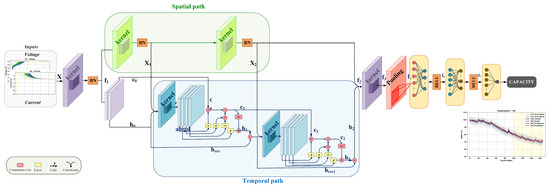
Figure 1. Proposed Dual Path Convolutional Residual LSTM Network model for SOH estimation.

The proposed model is evaluated using four NASA battery datasets (B5, B6, B7, B18) under two scenarios: (1) Same-Battery Evaluation and (2) Leave-One-Battery-Out Cross-Battery Generalization. In first experiment 60% of cycle data is used for training, while the remaining 40% is used for test. To further assess the model’s robustness and generalization capability, in the second experiment, a cross-validation strategy is employed, where one battery dataset is used for training while the remaining three are used for testing. The results demonstrate strong accuracy, robustness, and efficiency, further supported by extensive ablation studies quantifying the contribution of each architectural component. Edge-deployment tests on an NVIDIA Jetson AGX Orin confirm real-time feasibility with low latency, small memory footprint, and modest power consumption.

The remainder of this paper is as follows: Section 2 provides a review of SOH estimation problem. Section 3 describes the proposed model architecture in detail, explaining the role of each component in the estimation process. Section 4 presents model evaluation experiments and results. Section 5 is attributed to ablation studies and their evaluation and comparison from various practical perspectives. Section 6 concludes the paper with a discussion of future work.

2. SOH Estimation

LiBs undergo unavoidable aging during operation. Aging patterns are influenced by factors such as cell manufacturing characteristics and external conditions like ambient temperature, humidity, charge/discharge currents, and depth of discharge. Moreover, variations in electrode types and internal materials significantly affect aging. LiBs’ complex internal electrochemical processes are dynamic, nonlinear, and time-dependent. Alongside primary reactions, aging-induced side reactions occur and often interact through complex coupling mechanisms, further complicating aging. The interplay of electrochemical, thermal, and mechanical degradation processes results in nonlinear aging behavior, making long-term performance and reliability prediction difficult. Limited lifespan remains a major obstacle to large-scale commercialization. However, effective BMS strategies, such as accurate state estimation, predictive lifetime modeling, and proactive degradation mitigation, can help extend battery life. Globally, various policies are being introduced to improve health management. Notably, California’s Advanced Clean Cars II Regulations mandate the inclusion of a standardized SOH dashboard indicator starting in 2026, underscoring the growing importance of providing battery health information to drivers [1,14].

Mathematically, SOH is calculated as the ratio of the current battery capacity to its initial value:

$$SOH={\displaystyle \frac{C_{Current}}{C_{Initial}}}\times 100$$

(1)

where $C_{Current}$ and $C_{Initial}$ denote the current and initial capacity of a battery, respectively.

Battery health prognostic methods in the literature typically fall into three categories: model-based, data-driven, and hybrid approaches. At the current cycle, SOH aims to estimate capacity at that specific time. Accurate estimation provides the current health status of the battery, updates key parameters for short-term state estimates like SOC, and supports optimal management strategy design. Models for SOH estimation include empirical models, ECMs, and Electrochemical Models (EMs). Generally, model accuracy and complexity increase from empirical models to ECMs and then to EMs. However, empirical models lack physical interpretability. ECMs offer a balance between accuracy and complexity, making them widely used, while EMs provide high accuracy but are computationally intensive. The goal of model-based approaches is to construct models that effectively capture battery behavior and estimate representative parameters. It’s essential to balance model complexity and accuracy for real-time, embedded applications. Early detection of capacity drops enables timely maintenance and prevents further damage. Consequently, model-free ML-based methods, which aim to map nonlinear relationships between selected inputs and SOH, have gained popularity [1,2,3,15].

In this study, a dual-path DL-based algorithm is introduced for SOH estimation of LiBs, which is presented in more detail in the next section.

3. Proposed Model

Neural network algorithms can be categorized into recurrent and non-recurrent types. Recurrent algorithms retain memory of past data, while non-recurrent ones rely solely on the current data for processing. Although FNN generally have lower computational demands compared to methods like LSTM networks and Kalman Filters, it might lack the required accuracy for more complex tasks. The LSTM network improves memory retention of past data while Kalman filter, as one of the popular model-based methods in this area, has risks like negative covariance matrices, slow convergence, and large estimation errors in strongly nonlinear systems [2,16,17].

In this study, a dual-path convolutional residual LSTM network is proposed for SOH estimation, combining CNN and LSTM layers to effectively handle both spatial and temporal data features. Figure 1 illustrates the model architecture. The CNN layers extract spatial and local features such as charge-discharge patterns and voltage-current variations within each cycle. These features are then passed to ConvLSTM layers, which capture temporal dependencies, track degradation trends over time, and keep long-term dependencies. LSTMs are well-suited for modeling gradual degradation by leveraging both current and historical data. The dual-path structure processes different aspects of the data in parallel, enabling the model to capture both short-term fluctuations and long-term degradation independently. This enhances efficiency and allows for flexible fusion of high- and low-level features, which is essential as degradation manifests both gradually and variably. Inter-path connections regulate learning by combining different feature representations. CNN outputs are fed into the LSTM blocks, and the outputs of both paths are concatenated before the final layers. This prevents dominance by a single branch, leading to more stable and generalized predictions. Residual connections further improve gradient flow and feature extraction by mitigating vanishing gradients, helping preserve early degradation information critical for accurate predictions. They also regulate the information flow between CNN and LSTM components. LSTMs selectively regulate features, adjusting attention to degradation patterns over time. This adaptive memory structure enables the model to emphasize or suppress features as needed, enhancing SOH tracking. The integration of residuals and LSTMs strengthens representation learning while mitigating overfitting, a common issue in SOH tasks with limited labelled data. Specifically, residual connections add each block’s input to its output within the same time step, effectively merging representations across network depths. This helps preserve low-level degradation patterns. Additionally, ConvLSTM is used instead of regular LSTM, incorporating convolutional operations that better handle spatial dependencies in sequential battery data. ConvLSTM captures both spatial and temporal patterns, reduces parameter count through weight sharing, and supports more efficient learning for high-dimensional inputs. This structure also facilitates parallel computation. Unlike models requiring explicit feature engineering, this end-to-end model jointly learns feature extraction through CNNs and temporal regulation through LSTMs, improving SOH estimation performance.

The model’s formulation is as described in the following. k, s, and p stand for kernel, stride, and padding size in the presentations, respectively. The model receives two multi-channel 1D signals: voltage and current. Each signal has 3 channels, so the combined input is as below, where B and L are batch size and input sequence length, respectively, and 3 is the number of input channels as explained.

$$\mathbf{x}\in {\mathbb{R}}^{B\times 6\times L}$$

(2)

The input is passed through the first CNN block with k, s, and p set to 30, 4, and 0, respectively. The output called $f_1$ has 8 channels and is calculated as below, with BN standing for Batch Normalization. $L_1$ is output’s sequence length:

$$f_1=\mathrm{BN}\left(\mathrm{Conv}1\mathrm{D}\left(x\right)\right)\in {\mathbb{R}}^{B\times 8\times L_1}$$

(3)

In the temporal path, these eight channels are utilized to initialize the cell state and hidden state of the first ConvLSTM, with the first four channels assigned to the cell state and the remaining four to the hidden state:

$$c_0=f_1[:,:4,:],c_{t-1}\in {\mathbb{R}}^{B\times 4\times L_1}$$

(4)

$$h_0=f_1[:,4:,:],h_{t-1}\in {\mathbb{R}}^{B\times 4\times L_1}$$

(5)

In parallel, $f_1$ is fed into the spatial path with CNN block’s k, s, and p equal to 3, 1, and 1, respectively. The number of channels is kept at 8. Thus, the dimension does not change. The output of the first CNN block in the spatial path is the input of first ConvLSTM block in temporal path, calling it $X_1$:

$$X_1=\mathrm{BN}\left(\mathrm{Conv}1\mathrm{D}\left(x\right)\right)\in {\mathbb{R}}^{B\times 8\times L_1}$$

(6)

The output $X_1$ concatenated with $h_0$ is input to the first ConvLSTM cell, along with the previous states $c_{t-1},h_{t-1}\in {\mathbb{R}}^{B\times 4\times L_1}$. Unlike traditional LSTMs, this cell uses dilated 1D convolutions to exploit local and context-aware features. The convolution operation maps the input to 4 gates in a parallel operation mode that improves practical implementation:

$$z=\mathrm{Conv}1\mathrm{D}(X_1+h_{t-1})\in {\mathbb{R}}^{B\times 16\times L_1}$$

(7)

z is split along the channel dimension into four gates:

$$[a,b,g,d]=\mathrm{Split}(z,\dim =1),a,b,g,d\in {\mathbb{R}}^{B\times 4\times L_1}$$

(8)

a, b, g, and d correspond to forget gate, output gate, input gate, and candidate cell state, respectively. Then, each gate is passed through a nonlinearity using sigmoid function $\sigma (·)$. Then the update is implemented:

$${\mathbf{c}}_t=\mathbf{a}\odot {\mathbf{c}}_{\mathbf{t}-\mathbf{1}}+\mathbf{g}\odot \mathbf{d}$$

(9)

$${\mathbf{h}}_t=\mathbf{b}\odot tanh\left({\mathbf{c}}_t\right)$$

(10)

Following a similar procedure, in spatial path $X_1$ is passed through another CNN, reducing the number of channels to 4 from 8 and outputs $X_2$ with k, s, and p set to 3, 1, and 1, respectively:

$$X_2=\mathrm{BN}\left(\mathrm{Conv}1\mathrm{D}\left(X_1\right)\right)\in {\mathbb{R}}^{B\times 4\times L_1}$$

(11)

The second ConvLSTM receives $X_2$ and previous ConvLSTM output states and outputs $c_2$ and $h_2$ through a similar approach using residual connections. Then the results of the temporal path after addition with the $h_{res1}$ are concatenated with spatial path output:

$$f_2=\mathrm{Concat}(X_2,h_1)\in {\mathbb{R}}^{B\times 8\times L_1}$$

(12)

Next steps of convolution ($k=5$, $s=4$, and $p=0$), downsampling ($k=3$ and $s=2$), and following fully connected (fc) layers can be formulated as below:

$$f_3=\mathrm{Conv}1\mathrm{D}\left(f_2\right)\in {\mathbb{R}}^{B\times 4\times L_2},L_2=⌊{\displaystyle \frac{L_1-5}{4}}+1⌋$$

(13)

$$f_4=\mathrm{Pooling}\left(f_3\right)\in {\mathbb{R}}^{B\times 4\times L_3},L_3=⌊{\displaystyle \frac{L_2-3}{2}}+1⌋$$

(14)

After flattening and fc layers, the capacity C is predicted and used for SOH estimation:

$$\begin{array}{cc}\hfill f_5& =\mathrm{Flatten}\left(f_4\right)\in {\mathbb{R}}^{B\times (4·L_3)}\hfill \end{array}$$

(15)

$$\begin{array}{cc}\hfill f_6& =\mathrm{ReLU}\left(\mathrm{fc}\left(f_5\right)\right)\in {\mathbb{R}}^{B\times 16}\hfill \end{array}$$

(16)

$$\begin{array}{cc}\hfill f_7& =\mathrm{ReLU}\left(\mathrm{fc}\left(f_6\right)\right)\in {\mathbb{R}}^{B\times 8}\hfill \end{array}$$

(17)

$$\begin{array}{cc}\hfill C& =\mathrm{fc}\left(f_7\right)\in {\mathbb{R}}^{B\times 1}\hfill \end{array}$$

(18)

To summarize, the proposed architecture integrates convolutional layers for spatial pattern extraction with ConvLSTM units for temporal modeling, supported by residual and inter-path connections for stable feature flow. The model uses 4 intermediate channels throughout its convolutional and ConvLSTM layers. The first convolutional block ($k=30$, $s=4$, and $p=0$) reduces the sequence length while preserving a large temporal receptive field, enabling the ConvLSTM layers to focus on high-level aging patterns. All subsequent convolutional blocks use $k=3$, $s=1$, and $p=1$ to refine features while maintaining temporal resolution. Both ConvLSTM cells employ kernel size 3 with dilation 2 (padding 2), resulting in an effective temporal receptive field of 5 samples per each recurrent step. The fusion convolution uses $k=5$, $s=4$, and $p=0$ to compress the concatenated spatial–temporal representation prior to pooling. A final average-pooling layer ($k=3$ and $s=2$) reduces the sequence length before the fully connected layers. The prediction head consists of linear layers of sizes $4L_3$→16→8→1, with ReLU activations between layers.

4. Model Evaluation and Results

To evaluate the model, it needs to be tested with real-world data. Several publicly available battery datasets can be used, and in this work, the NASA dataset is employed. Among them, B5–B7 and B18 are the most commonly used. These datasets capture cyclic aging through following test conditions: constant current–constant voltage (CC-CV) charging, constant current (CC) discharging, and impedance spectrum testing. During the charging process, each battery is charged at 1.5 A until it reaches 4.2 V, and then held at constant voltage until the current drops below 20 mA. Discharging is carried out at 2 A until the battery voltages reach specific endpoints 2.7, 2.5, 2.2, and 2.5 V for each respective battery. It is clear that batteries have different discharge cut-off voltages. Moreover, the initial capacity for various cells is not the same. It is 1.8565, 2.0353, 1.89105, and 1.85501 Ah for B5, B6, B7, and B18, respectively. It should be noted that no initial-capacity normalization or cross-battery calibration was performed. The model was trained and evaluated using the measured capacities directly, without scaling each cell’s data to a common reference. This design choice reflects real-world conditions in which the initial capacity of a deployed cell is typically unknown. As a result, the reported inter-cell variations also capture the model’s robustness to intrinsic differences among batteries.

These tests are repeated until each battery reaches a 30% capacity loss, marking the end of its life. The number of cycles before reaching 70% of initial capacity and the number of data points in each cycle vary across batteries, confirming their different behavior. It is 167 cycles for B5–B7 and 132 cycles for B18. Figure 2 illustrates the battery capacity as a function of cycle count for these datasets. Moreover, Figure 3 illustrates charge current and voltage signals across batteries and during their lifespan, highlighting their different aging behavior. Besides, Figure 4 shows the voltage profile for one cycle of all batteries over time in terms of time and sample, highlighting inconsistencies in sampling frequency and duration.

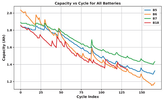
Figure 2. NASA batteries 5, 6, 7, and 18 capacities per cycle.

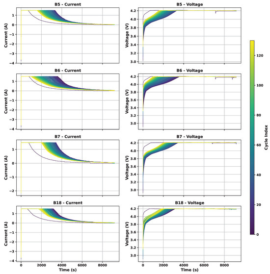
Figure 3. Batteries charge current and voltage signals during the aging process.

Figure 4. Same cycle in various cells in terms of time and sample.

To standardize the time, interpolation is performed with a step size of three seconds, ensuring all data aligns to the same time frame. This interval was selected through empirical evaluation: shorter steps (e.g., 1 s) yielded redundant samples with minimal information gain, whereas larger steps (e.g., 5 s) smoothed out critical transient features that contribute to accurate SOH estimation. Additionally, cycles do not stop at a fixed time. Thus, after interpolation, each cycle is extended to the maximum duration observed across all batteries by padding with the last recorded value. Since such padding introduces long flat regions that carry no degradation information and differ in length between batteries, the sequences are cropped at 3500 points to avoid redundant constant values at the cycle ends. This threshold preserves all meaningful transient and mid-cycle patterns while removing extended flat tails that would otherwise dominate the sequence and bias learning. Following interpolation and cropping, the data are arranged into three parallel channels. This approach ensures that the last data points of shorter cycles are placed in a separate channel and isolated, distinct from the meaningful data in the initial channel. The first channel contains the main transient sequence, while the additional channels isolate regions that include mid-cycle and padded or less informative flat segments. This multi-channel representation enables the network to assign different importance to transient, middle, and flat portions of the cycle, preventing padded values from interfering with informative sections of the data. It also facilitates efficient parallel processing, improving both learning stability and computational performance. Below pseudo code in Algorithm 1 presents the steps [18].

Algorithm 1 Preprocessing and three-channel construction for each charge cycle

Require:  Raw time stamps $t_c$, voltage $v_c$, current $i_c$ for cycle c; Interpolation step $\mathrm{\Delta }t=3$ s; Maximum charge duration $t_{max}$ across all batteries; Cropped length $L_{\mathrm{crop}}=3500$ samples. Ensure:  Six-channel input $x_c\in {\mathbb{R}}^{6\times L_{\mathrm{seg}}}$ for cycle c. 1: Construct uniform time grid: $t_{\mathrm{grid}}\leftarrow [0,\mathrm{\Delta }t,2\mathrm{\Delta }t,\dots ,t_{max}]$. 2: Interpolate voltage and current onto $t_{\mathrm{grid}}$:             $v_{\mathrm{interp}}\leftarrow \mathrm{Interp}(t_c,v_c,t_{\mathrm{grid}})$, $i_{\mathrm{interp}}\leftarrow \mathrm{Interp}(t_c,i_c,t_{\mathrm{grid}})$. 3: if  $\mathrm{len}\left(v_{\mathrm{interp}}\right)>L_{\mathrm{crop}}$  then 4:             Truncate to remove long flat tails:             $v_{\mathrm{interp}}\leftarrow v_{\mathrm{interp}}[0:L_{\mathrm{crop}}]$, $i_{\mathrm{interp}}\leftarrow i_{\mathrm{interp}}[0:L_{\mathrm{crop}}]$. 5: else if  $\mathrm{len}\left(v_{\mathrm{interp}}\right)<L_{\mathrm{crop}}$  then 6:             Pad with last value:             $v_{\mathrm{last}}\leftarrow v_{\mathrm{interp}}[-1]$, $i_{\mathrm{last}}\leftarrow i_{\mathrm{interp}}[-1]$. 7:             while $\mathrm{len}\left(v_{\mathrm{interp}}\right)<L_{\mathrm{crop}}$ do 8:                    Append $v_{\mathrm{last}}$ to $v_{\mathrm{interp}}$. 9:                    Append $i_{\mathrm{last}}$ to $i_{\mathrm{interp}}$. 10:             end while 11: end if 12: Compute segment length: $L_{\mathrm{seg}}\leftarrow ⌊{\displaystyle \frac{L_{\mathrm{crop}}}{3}}⌋$. 13: Split interpolated signals into three contiguous temporal segments:             $v_1\leftarrow v_{\mathrm{interp}}[0:L_{\mathrm{seg}}]$, $v_2\leftarrow v_{\mathrm{interp}}[L_{\mathrm{seg}}:2L_{\mathrm{seg}}]$, $v_3\leftarrow v_{\mathrm{interp}}[2L_{\mathrm{seg}}:3L_{\mathrm{seg}}]$;             $i_1\leftarrow i_{\mathrm{interp}}[0:L_{\mathrm{seg}}]$, $i_2\leftarrow i_{\mathrm{interp}}[L_{\mathrm{seg}}:2L_{\mathrm{seg}}]$, $i_3\leftarrow i_{\mathrm{interp}}[2L_{\mathrm{seg}}:3L_{\mathrm{seg}}]$. 14: Form six-channel input by stacking voltage and current segments:             $x_c\leftarrow [v_1;v_2;v_3;i_1;i_2;i_3]\in {\mathbb{R}}^{6\times L_{\mathrm{seg}}}$. 15: return $x_c$.

In addition to voltage and current, the NASA dataset also provides temperature measurements recorded at approximately room temperature (24 °C) with minimal variation throughout cycling. We evaluated the effect of incorporating temperature as an additional input channel; however, due to the near-constant thermal conditions, temperature contributed no additional information and did not improve performance in either Experiment I or Experiment II. For fairness and to maintain a practical sensing requirement aligned with real-world deployment, particularly charging-station environments and upcoming SOH dashboard regulations, we deliberately restricted the model input to voltage and current only. Temperature can be incorporated in multi-condition datasets, and its integration is discussed as part of future work.

The model is evaluated using two experiments. Both experiments use the same training configuration. An Adam optimizer with a batch size of 50 and a fixed learning rate of 0.001 is employed, and the mean squared error of the predicted capacity is used as the loss function. No learning-rate scheduler, dropout, or weight decay is applied. Hyperparameters such as learning rate and batch size were selected through preliminary empirical testing over a small set of candidate values, prioritizing stable convergence and low validation error while maintaining a compact model suitable for edge implementation. In the first Same-Battery Evaluation, 60% of the data from a single battery is used for training, and the remaining 40% for testing (Figure 5 and Table 1). The data are kept in their original chronological order without any random shuffling, since the NASA battery degradation dataset represents a time-dependent process where the sequence of cycles contains essential degradation information. Preserving the temporal order avoids information leakage from future cycles and ensures realistic performance evaluation. In Cross-Battery Generalization, a battery-level cross-validation strategy is employed. In each fold, the model is trained using the complete data from one battery and tested on the remaining three batteries that exhibit different degradation behaviors (Figure 3). This Leave-One-Battery-Out (LOBO) scheme simultaneously maintains the temporal dependency within each battery and evaluates the model’s generalization to unseen operating conditions. It should be noted that no initial-capacity normalization or inter-cell calibration was applied to reflect realistic deployment conditions, as the true initial capacity of a battery is typically unknown in practical settings.

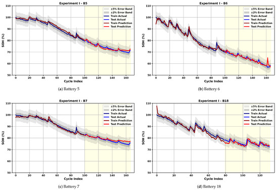
Figure 5. Same-Battery Evaluation: SOH estimation results using 60% of the same cell’s data for training and the remaining 40% for test.

Table 1. SOH estimation results—Same-Battery Evaluation.

Train						Test
B	E	RMSE%	MAE%	${\mathit{R}}^{\mathbf{2}}$		RMSE%	MAE%	${\mathit{R}}^{\mathbf{2}}$
5	1000	1.173	1.032	0.965		0.994	0.833	0.895
6	302	1.527	1.096	0.973		1.400	0.861	0.870
7	736	1.031	0.739	0.967		1.225	0.959	0.766
18	1227	1.611	1.220	0.925		1.415	1.096	0.386
Mean	816	1.335	1.022	0.957		1.258	0.937	0.729

To ensure statistical robustness, all performance metrics, Root Mean Squared Error (RMSE), Mean Absolute Error (MAE), and coefficient of determination ($R^2$), are reported as the mean ± standard deviation across the four LOBO folds. Results are presented in Figure 6, Figure 7, Figure 8 and Figure 9 and Table 2.

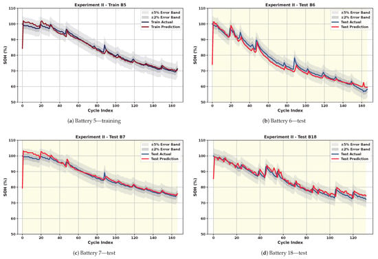
Figure 6. Cross-Battery Generalization: SOH estimation results using B5 for training and the other three cells for test.

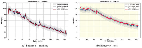
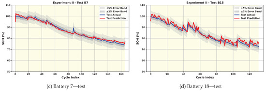
Figure 7. Cross-Battery Generalization: Cross-Battery Generalization: SOH estimation results using B6 for training and the other three cells for test.

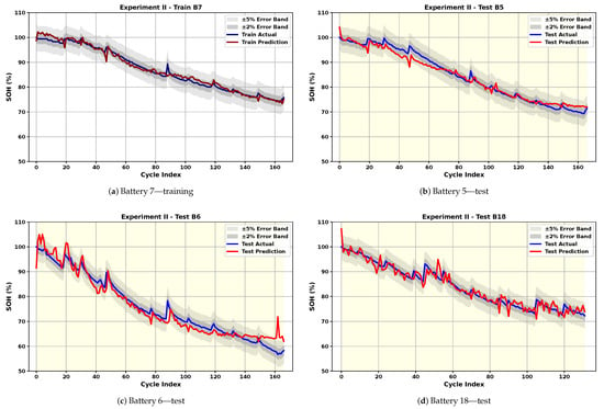
Figure 8. Cross-Battery Generalization: SOH estimation results using B7 for training and the other three cells for test.

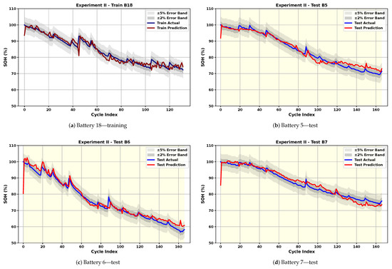
Figure 9. Cross-Battery Generalization: SOH estimation results using B18 for training and the other three cells for test.

Table 2. SOH Estimation Results—Cross-Battery Generalization.

	Train		Test				Train		Test				Train		Test				Train		Test
	B5		B6	B7	B18		B6		B5	B7	B18		B7		B5	B6	B18		B18		B5	B6	B7
RMSE%	1.772		2.784	2.139	2.145		1.729		1.479	1.191	2.386		1.268		1.835	2.998	2.290		2.099		1.902	2.476	2.085
MAE%	1.084		1.688	1.196	1.527		1.051		1.148	0.884	1.910		0.958		1.356	2.218	1.614		1.498		1.389	1.661	1.616
$R^2$	0.970		0.949	0.937	0.933		0.980		0.979	0.980	0.918		0.978		0.968	0.941	0.924		0.936		0.966	0.960	0.940
E	232						251						342						755
		E			Train RMSE%				Train MAE%		Train $R^2$				Test RMSE%			Test MAE%			Test $R^2$
Mean		395			1.717				1.148			0.966			2.143			1.517			0.950
Std		245			0.342				0.240			0.020			0.321			0.173			0.009

As shown in Figure 5, the model successfully captures the overall degradation trend and even follows abrupt capacity changes with high accuracy. Table 1 reports that the test RMSE and MAE range from 0.99% to 1.41% and 0.74% to 1.22%, respectively. Additionally, the model converges within an average of 816 epochs across all batteries, showcasing its computational efficiency. The average test RMSE and MAE are 1.26% and 0.94%, respectively, reflecting consistent and reliable performance. Among the batteries, B18 presents the greatest challenge for the model due to its higher fluctuations. This is evident from the increased test error and the greater oscillations observed in its predictions. The low $R^2$ scores for B7 and B18 are attributed to the limited variance of the actual SOH data in the final 40% of cycles, where even small RMSE values can yield low $R^2$ due to its dependence on the ratio of prediction error to label variance. Although $R^2$ is reported in Table 1 for completeness, its interpretation must be treated cautiously in low-variance regions. $R^2$ is computed as

$$R^2=1-{\displaystyle \frac{{\sum }_{i=1}^N{(y_i-{\widehat{y}}_i)}^2}{{\sum }_{i=1}^N{(y_i-\overline{y})}^2}},$$

(19)

where $y_i$ denotes the true SOH, ${\widehat{y}}_i$ the predicted SOH, and $\overline{y}$ the mean of the true SOH in the test region. The denominator $\sum {(y_i-\overline{y})}^2$ is proportional to the variance of the true SOH; therefore, when this variance is small, $R^2$ becomes highly sensitive to even small absolute errors. The SOH variances in the test regions for B5, B6, B7, and B18 are 9.39, 15.10, 6.42, and 3.26, respectively. In particular, B18 exhibits the smallest variance, and the SOH values lie within a narrow range in the final 40% of its cycles. This leads to a small denominator and a correspondingly low $R^2$ value (0.386), despite RMSE and MAE being comparable to those of the other cells. For practical battery-management applications and regulatory thresholds, absolute-error metrics such as RMSE and MAE are more meaningful indicators of performance than correlation-based metrics. This is further reflected in Experiment II, where larger SOH variability yields both higher $R^2$ and low RMSE, demonstrating that the proposed model accurately tracks degradation trends when sufficient signal variance is present.

In Cross-Battery Generalization, model’s robustness and ability to generalize across different battery cells with limited training data are tested. As expected, this is a more challenging task, and results in slightly less smooth predictions, as seen in Figure 6, Figure 7, Figure 8 and Figure 9. Despite this, the model maintains strong performance. Table 2 shows that even in the most challenging scenario, the test RMSE and MAE do not exceed 2.99% and 2.22%, respectively, underscoring the model’s ability to generalize across battery types without significant performance degradation. The average test RMSE and MAE across all scenarios are 2.14% and 1.52%, respectively. This result is achieved within an average of 395 epochs over all four scenarios. The small gap between training and testing performance, along with a high average test $R^2$ score of 0.95, confirms the model’s strong generalization capability across different batteries. However, it is evident that the results vary depending on the training battery. When B18, which has fewer cycles, or B5 and B7, which exhibit smoother behavior, are used for training, the test performance on the remaining batteries degrades. This highlights the importance of selecting training data that encompasses a variety of scenarios and behaviors.

A factor influencing the results is the difference in the initial capacities of the cells, as well as inconsistent cutoff discharge voltages across batteries. The test RMSE for battery B6 is the highest when trained with either B5 or B7. This can be attributed to the distinct behaviors of the cells, in addition to the higher initial capacity of B6 (2.0353 Ah) compared to B5 (1.8565 Ah). In contrast, when B6 is used for training, the RMSE for B5 and B7 is much lower, while B18 still shows a higher error, likely due to its different number of cycles. This observation suggests that DL models are generally more effective at interpolation than extrapolation.

Alongside these observations, the cross-battery results are influenced by inherent differences across NASA cells, including initial capacities (1.856–2.035 Ah), discharge cutoff voltages (2.2–2.7 V), and total cycle counts (132–167). These variations lead to differences in the shape, duration, and smoothness of the charge curves, resulting in distinct degradation behaviors. When training is performed on batteries with smoother degradation trajectories (e.g., B5 or B7), the model is exposed to narrower feature distributions, and testing on more irregular cells (e.g., B6 or B18) requires extrapolation beyond the observed range, which increases prediction error. Conversely, training on B6, which exhibits both gradual decline and localized fluctuations, provides a richer set of patterns and yields the strongest average cross-battery R². Although the present study focuses on strict one-battery training scenarios, future work may investigate mixed-battery training or data augmentation strategies to reduce the gap between intra-battery and cross-battery performance. To further examine how dataset characteristics influence cross-battery performance, the PCC was computed between several battery descriptors, initial capacity, discharge cutoff voltage, and cycle count, and the average test RMSE obtained when training on each cell. The results show a strong negative correlation between initial capacity and test error (PCC = −0.896), indicating that batteries with higher initial capacity, such as B6, tend to provide more informative training data and yield better generalization. In contrast, cutoff voltage (PCC = −0.135) and cycle count (PCC = −0.024) exhibit negligible correlation with test error, suggesting that these factors play a minor role within the controlled NASA dataset. Additionally, visual inspection of Figure 4 shows that B6 exhibits the widest variation in charge current and voltage profiles across aging, providing a more diverse set of patterns for the model to learn from. This broader temporal variability appears to facilitate generalization, resulting in superior cross-battery performance when B6 is used for training compared to smoother batteries such as B5 or B7. Among the four NASA cells, B6 demonstrates the best cross-battery generalization performance. This can be attributed to the fact that B6 exhibits a broader range of charge–discharge dynamics across aging, including more pronounced temporal shifts in the constant-current and constant-voltage phases (Figure 4). These cycle-to-cycle variations expose the model to a richer set of degradation signatures during training, enabling it to learn more diverse representations. In contrast, batteries such as B5 and B7 follow smoother and more uniform degradation patterns, providing narrower feature distributions for the model to learn from. As a result, models trained on B6 generalize more effectively to unseen cells with different behaviors.

Additionally, because all NASA cells were cycled at approximately room temperature (24 °C), the dataset lacks environmental diversity. This may limit generalization to real EV applications, where temperature, load profiles, and operational conditions vary widely. Expanding evaluation to multi-temperature datasets is therefore an important direction for future work.

An important observation across both experiments is that the model exhibits a higher estimation error during the first recorded cycle. This occurs because, in the NASA dataset, the first charge cycle of each cell does not begin from a fully discharged state. As illustrated in Figure 3, the voltage and current trajectories in this cycle differ markedly from all subsequent cycles, making it an outlier relative to the long-term aging trend. Since the model is trained on consistent charge–discharge patterns, this irregular initial cycle leads to a deviation in the predicted SOH. Additionally, in some early cycles, SOH values slightly above 100% are observed. This arises naturally from the capacity-regression formulation, where SOH is computed as the ratio between the predicted capacity and the initial capacity; small positive prediction bias when the cell is still near its nominal state can therefore exceed 100%. Differences in initial capacities across cells (1.855–2.035 Ah for B5–B18) may also contribute to small offsets in cross-cell normalization. Although such anomalies could be mitigated through post-processing (e.g., clipping SOH to [0, 100]%) or through bounded-output strategies such as sigmoid-scaled regression, we intentionally avoid these adjustments to preserve the data’s original structure and to transparently show the model’s behavior under non-ideal conditions. Both approaches would artificially constrain the output and mask informative deviations and trends, particularly in cross-battery settings where SOH may legitimately exceed 100%. Bounded regression using a sigmoid output can constrain SOH to the range [0, 100]%; however, doing so requires training targets to be normalized by the initial capacity. Since our formulation deliberately avoids using initial capacity, as it is often unknown or unavailable in practical settings, sigmoid-based outputs are not appropriate for this capacity-regression framework. Importantly, aside from these early-cycle irregularities, the model remains stable and accurate throughout the remainder of each cell’s lifespan, which better reflects real-world operation where early-cycle inconsistencies may arise from manufacturing variation or incomplete conditioning.

To demonstrate the advantages of the proposed model over existing methods in the literature, Table 3 provides a comparison from multiple perspectives. V, I, T, and C denote voltage, current, temperature, and capacity, respectively. To ensure a fair interpretation, it is important to recognize that the referenced works differ in their input requirements, assumptions, and data usage. Several studies, including [4,7], rely on richer sensing modalities such as discharge voltage/current, temperature, or incremental capacity features. Method [8] additionally incorporates historical capacity values and therefore requires knowledge of the initial capacity, which is typically unavailable in real-world implementations. In contrast, the proposed model operates under a stricter and more practical setting: it uses only charge-cycle voltage and current, does not rely on temperature, discharge data, or initial-capacity information, and is trained with only 60% of the available cycles. Furthermore, some existing works also do not report model size, number of epochs, or computational cost, which limits the ability to perform quantitative efficiency comparisons, an important factor for deployment in embedded systems. Among those that do report complexity, most use significantly larger models than ours. Furthermore, several models in the literature are not implemented in an end-to-end manner or do not evaluate cross-battery generalization. Compared to [8], which is the only other method that avoids HI extraction, the proposed model achieves a slightly higher RMSE; however, this is obtained using substantially less input information and with a far smaller model, making it more suitable for embedded system applications. Our network has only 4913 trainable parameters, operates end-to-end, and demonstrates stable performance on unseen batteries. Although cross-validation was performed in this study, the results are not reported because validation was conducted across different batteries, making direct comparison with works that validate on the same cell unfair. Overall, the proposed architecture provides a favorable balance of accuracy, minimal sensing requirements, and low model complexity, making it well-suited for resource-constrained and real-world deployment scenarios.

Table 3. Proposed model’s performance compared to other works, ✓= yes/included; ✗= no/not included.

Model	End-to-End	Training Data	Training Data	RMSE (%)	Cross RMSE (%)	No. of Parameters
Proposed	✓	Charge V and I	60%	1.3	2.1	4913
[4]	✗	Charge and discharge V, I, and T	60%	0.7	✗	-
[5]	✗	Charge V and I	140 cycles B0005	6.7	✗	-
[7]	✗	Charge V, I, T, and incremental C	60%	0.6	✗	62,101
[8]	✓	Discharge V, I, T, historical C	70%	0.33	✓	14,000

To evaluate the feasibility of deploying the proposed model in real-time edge scenarios, inference was implemented on an NVIDIA Jetson AGX Orin Developer Kit (model P3730). The input was structured to match the training configuration, consisting of six channels derived from voltage and current signals. Multiple test runs were conducted, each including 10 warm-up iterations followed by 100 timed inference runs. Across these trials, the model consistently achieved an average inference latency of approximately 3.22–3.72 ms per prediction, with GPU memory usage of 8.24 MB allocated and 22.00 MB reserved. These results demonstrate the model’s suitability for real-time battery SOH monitoring on resource-constrained embedded platforms, enabling low-latency and low-power operation without relying on cloud infrastructure.

5. Ablation Study

To further clarify the contribution of each component in the proposed Dual-Path ConvLSTM architecture, several ablation studies were performed under the cross-battery generalization setting (Cross-Battery Generalization). In all cases, the training, validation, and testing configurations were kept identical to the full model to ensure that differences in results arise solely from structural modifications rather than data configuration. Specifically, the effects of (i) the dual-path design versus single-path baselines, (ii) ConvLSTM versus standard LSTM, (iii) residual and inter-path connections, and (iv) the preprocessing and three-channel input structure are quantified. Results are reported as mean and standard deviation across folds.

The proposed full Dual-Path ConvLSTM+CNN model with residual and inter-path connections attains a test RMSE of 2.143 ± 0.321%, MAE of 1.517 ± 0.173%, and $R^2$ of 0.950 ± 0.009 within 395 ± 245 epochs (mean ± std), establishing the reference for comparison. This ablation suite quantifies the contribution of each component and explains the observed gains in performance, training efficiency, and robustness under cross-battery evaluation.

5.1. Dual-Path Structure

To evaluate the effectiveness of the dual-path design, each path was independently disabled while keeping all other parameters constant. When only the ConvLSTM (Table 4) path or only the convolutional (Conv) path was used, the performance degraded noticeably in both training and testing phases. The single-path variants required considerably more epochs (on average more than twice as many) to converge and exhibited larger discrepancies between training and testing metrics, indicating weaker generalization capability.

Table 4. SOH Estimation Ablation Study—Cross-Battery Generalization—Only Temporal Path.

	Train		Test				Train		Test				Train		Test				Train		Test
	B5		B6	B7	B18		B6		B5	B7	B18		B7		B5	B6	B18		B18		B5	B6	B7
RMSE%	1.276		2.287	1.560	3.116		1.330		2.811	2.082	2.472		2.450		2.529	3.376	1.982		2.439		2.123	4.121	1.582
MAE%	0.924		1.541	1.118	2.676		0.809		2.238	1.867	1.989		2.160		1.785	2.650	1.507		1.515		1.587	2.801	1.016
$R^2$	0.985		0.966	0.966	0.860		0.989		0.925	0.940	0.912		0.917		0.939	0.926	0.943		0.914		0.957	0.889	0.965
E	501						675						1355						852
		E			Train RMSE%				Train MAE%			Train $R^2$			Test RMSE%			Test MAE%			Test $R^2$
Mean		846			1.874				1.352			0.951			2.503			1.898			0.933
Std		369			0.659				0.621			0.041			0.144			0.127			0.004

Table 5 presents the results obtained using only the Conv path (omitting the ConvLSTM path), showing a more significant degradation in the test performance, approximately double the training epochs, and lower $R^2$ values, reflecting higher prediction uncertainty. Moreover, the single-path structures demonstrated inconsistent behavior across batteries: for instance, when the training was performed on cell B18, the performance varied widely among the test batteries (e.g., RMSE ranging from 1.6% to 4.1%), highlighting poor robustness and weak cross-battery generalization.

Table 5. SOH Estimation Ablation Study—Cross-Battery Generalization—Only Spatial Path.

	Train		Test				Train		Test				Train		Test				Train		Test
	B5		B6	B7	B18		B6		B5	B7	B18		B7		B5	B6	B18		B18		B5	B6	B7
RMSE%	1.192		3.350	2.592	2.813		2.285		1.906	1.856	2.288		1.255		2.355	3.088	3.549		2.706		2.571	4.562	2.181
MAE%	0.821		2.642	1.921	2.108		1.942		1.605	1.579	1.735		0.801		2.008	2.180	1.507		1.857		1.895	3.497	1.138
$R^2$	0.987		0.927	0.907	0.886		0.966		0.965	0.952	0.924		0.978		0.947	0.938	0.818		0.894		0.937	0.864	0.934
E	884						1124						586						240
		E			Train RMSE%				Train MAE%			Train $R^2$			Test RMSE%			Test MAE%			Test $R^2$
Mean		709			1.860				1.355			0.956			2.759			1.985			0.917
Std		382			0.375				0.629			0.042			0.501			0.271			0.021

In contrast, the proposed dual-path configuration enables complementary feature extraction, where the Conv path captures spatial and local characteristics (e.g., voltage and current trends), and the ConvLSTM path models long-term temporal dependencies and degradation evolution. Their combination yields balanced spatio-temporal learning, faster convergence, higher accuracy, and improved robustness across different batteries.

5.2. ConvLSTM vs. Standard LSTM

To examine the role of ConvLSTM units, the convolutional recurrent blocks were replaced by standard LSTM layers while keeping the rest of the architecture unchanged (Table 6).

Table 6. SOH Estimation Ablation Study—Cross-Battery Generalization—Standard LSTM.

	Train		Test				Train		Test				Train		Test				Train		Test
	B5		B6	B7	B18		B6		B5	B7	B18		B7		B5	B6	B18		B18		B5	B6	B7
RMSE%	2.140		3.349	2.195	2.363		1.676		0.968	1.393	1.819		1.819		2.920	3.636	3.054		2.039		2.589	4.132	1.150
MAE%	1.470		2.232	1.586	1.745		1.062		0.695	1.075	1.357		1.331		2.341	2.546	2.459		1.444		2.107	3.389	0.865
$R^2$	0.957		0.927	0.933	0.919		0.982		0.991	0.973	0.952		0.954		0.919	0.914	0.865		0.940		0.936	0.889	0.982
E	841						1092						629						766
		E			Train RMSE%				Train MAE%			Train $R^2$			Test RMSE%			Test MAE%			Test $R^2$
Mean		832			1.918				1.327			0.958			2.464			1.783			0.933
Std		194			0.210				0.187			0.017			0.763			0.576			0.030

The LSTM-based model required significantly more epochs to converge (more than twice, on average) and exhibited larger variations in performance across folds and test batteries, indicating reduced robustness and slower or stiffer training dynamics in the absence of convolutional gating. Without the convolutional operations within the recurrent gates, spatial correlations among the input features are not preserved, leading to noisier gradients and less stable training. Conversely, the ConvLSTM mechanism integrates spatial filtering directly within temporal modeling, allowing the network to jointly learn both local spatial dependencies and long-term temporal evolution. This results in smoother training behavior, better cross-battery consistency, and stronger overall generalization.

5.3. Residual and Inter-Path Connections

The effect of residual (Table 7) and inter-path (Table 8) connections was analyzed next. Removing residual connections led to a noticeable decline in training stability and test performance, confirming that residual shortcuts maintain smooth gradient flow and prevent vanishing gradients during deep temporal modeling. Similarly, disabling the inter-path feature exchange slightly altered the training metrics but degraded the test performance and increased variability across batteries, reflecting reduced robustness. This indicates that inter-path regulation between the Conv and ConvLSTM branches enhances robustness, as these paths guide one another’s feature refinement and prevent over-specialization to a single battery’s pattern.

Table 7. SOH Estimation Ablation Study—Cross-Battery Generalization—Removing Residual Connections.

	Train		Test				Train		Test				Train		Test				Train		Test
	B5		B6	B7	B18		B6		B5	B7	B18		B7		B5	B6	B18		B18		B5	B6	B7
RMSE%	1.191		2.726	1.361	2.705		2.047		2.479	2.124	3.226		2.456		1.605	4.137	1.719		2.249		2.131	4.134	1.668
MAE%	0.801		2.089	0.943	2.052		1.530		1.911	1.735	2.616		2.198		1.325	2.661	1.342		1.754		1.836	3.120	1.330
$R^2$	0.987		0.952	0.974	0.894		0.973		0.942	0.938	0.850		0.917		0.976	0.888	0.957		0.927		0.957	0.888	0.962
E	311						345						206						345
		E			Train RMSE%				Train MAE%			Train $R^2$			Test RMSE%			Test MAE%			Test $R^2$
Mean		302			1.986				1.568			0.951			2.501			1.913			0.931
Std		66			0.556				0.584			0.034			0.172			0.208			0.014

Table 8. SOH Estimation Ablation Study—Cross-Battery Generalization—Removing InterPath Connections.

	Train		Test				Train		Test				Train		Test				Train		Test
	B5		B6	B7	B18		B6		B5	B7	B18		B7		B5	B6	B18		B18		B5	B6	B7
RMSE%	1.687		3.340	1.833	2.808		2.091		1.063	1.043	1.850		1.247		1.826	2.483	1.950		1.617		2.115	4.132	2.412
MAE%	1.226		2.526	1.268	2.205		1.390		0.761	0.845	1.468		1.061		1.355	1.771	1.446		1.285		1.799	3.452	1.934
$R^2$	0.973		0.927	0.954	0.886		0.972		0.989	0.985	0.951		0.979		0.968	0.888	0.945		0.962		0.958	0.889	0.920
E	288						624						293						665
		E			Train RMSE%				Train MAE%			Train $R^2$			Test RMSE%			Test MAE%			Test $R^2$
Mean		468			1.661				1.240			0.972			2.238			1.736			0.938
Std		205			0.346				0.138			0.007			0.699			0.593			0.025

Overall, both mechanisms primarily contribute to model stability and generalization rather than direct accuracy improvement, confirming their importance in achieving reliable cross-battery performance.

5.4. Preprocessing and Three-Channel Input Structure

Finally, the impact of preprocessing was evaluated by removing the interpolation/cropping step and the three-channel input design (Table 9). In this configuration, the model received unaligned sequences with varying cycle lengths across batteries, padded to the maximum length using the edge value of each cycle.

Table 9. SOH Estimation Ablation Study—Cross-Battery Generalization—Removing Preprocessing.

	Train		Test				Train		Test				Train		Test				Train		Test
	B5		B6	B7	B18		B6		B5	B7	B18		B7		B5	B6	B18		B18		B5	B6	B7
RMSE%	1.827		3.820	2.554	8.590		2.130		3.164	2.712	6.560		0.734		1.594	2.450	7.561		2.871		18.949	19.648	17.534
MAE%	0.999		2.364	1.679	7.553		1.193		2.879	2.417	4.988		0.526		1.168	1.779	6.396		2.167		15.418	16.220	13.220
$R^2$	0.968		0.905	0.910	−0.066		0.970		0.905	0.898	0.378		0.993		0.976	0.961	0.174		0.881		−2.415	−1.520	−3.247
E	30						106						257						92
		E			Train RMSE%				Train MAE%			Train $R^2$			Test RMSE%			Test MAE%			Test $R^2$
Mean		121			1.890				1.221			0.953			7.928			6.340			−0.095
Std		96			0.887				0.690			0.049			7.204			5.750			1.534

Without temporal alignment and channel separation, the model rapidly overfitted the training battery and failed to generalize to unseen ones. This behavior was especially severe when training on B18, which exhibits distinct degradation dynamics and sequence lengths. The degraded performance, large test errors, and even negative $R^2$ values confirm that time alignment and structured channelization are critical to maintaining cross-battery robustness.

The three-channel representation allows the model to separately capture transient, mid-cycle, and steady-state behaviors, enabling more structured and informative feature extraction. This confirms that the proposed preprocessing strategy is essential for effective cross-battery learning and consistent feature interpretation.

5.5. Takeaway

While each individual component contributes to the overall performance, the comparative studies clearly show that the full Dual-Path ConvLSTM model with residual and inter-path connections and the proposed three-channel preprocessing consistently achieves the best accuracy and stability on unseen batteries, while requiring fewer training epochs than the ablated variants. These results confirm that the improvements of the proposed model are directly attributable to its architectural innovations, synergistic dual-path feature learning, and robust preprocessing pipeline.

In addition to accuracy, the computational comparison further reinforces these observations. As summarized in Table 10, the proposed model maintains a compact parameter count (4913 trainables) comparable to or smaller than several ablated variants, yet converges more efficiently, with an average of 395 epochs, substantially fewer than the single-path or LSTM-based models that require 700–850 epochs to reach inferior accuracy. Real-time inference was evaluated on the NVIDIA Jetson AGX Orin under MAXN mode. The model achieved from training on B18 is employed. with power monitoring performed using the jtop utility. During idle conditions, the total power draw (ALL) was approximately 12.3 W, which increased during inference to 25.2 W, confirming an active power usage of 12.9 W for proposed model execution. All architectural variants exhibit similar memory allocation (around 8.2 MB), indicating that architectural differences do not impose additional memory overhead. The proposed method also achieves low inference latency (2.24 ms), outperforming the dual-path LSTM-Conv baseline, which incurs significantly higher latency (14.16 ms) due to its heavier sequential recurrence. Power consumption across all models remains comparable, demonstrating that the proposed architecture improves accuracy and latency without increasing energy requirements. Furthermore, results demonstrates that omitting the preprocessing stage results in slight increases in memory usage, latency, and energy consumption. This confirms that the proposed preprocessing and three-channel representation improve not only model robustness but also computational efficiency and resource management during embedded inference.

Table 10. Computational comparison across architectural variants on NVIDIA Jetson AGX Orin.

Model	No. of	Epochs	Train	Test	Worst Test	Memory	Inference	Total Energy
Variant	Trainables		RMSE%	RMSE%	RMSE%	(MB)	Latency (ms)	(W)
Proposed Method	4913	395	1.717	2.143	2.998	8.24	2.24	25.2
Dual Path LSTM-Conv	3689	832	1.918	2.464	4.132	8.22	14.16	27.3
Only Temporal	4217	846	1.874	2.503	4.121	8.22	2.01	27.3
Only Spatial	3225	709	1.860	2.759	4.562	8.21	1.25	27.3
Residual Removal	4913	302	1.986	2.501	4.137	8.24	2.00	27.4
Interpath Removal	5345	468	1.661	2.238	4.132	8.24	2.61	27.4
Preprocessing Removal	4433	121	1.890	7.928	19.648	8.29	2.27	27.3

Taken together, these results demonstrate that the full Dual-Path ConvLSTM architecture provides the best balance of accuracy, robustness, convergence speed, and embedded-device efficiency, validating its suitability for real-time and resource-constrained battery management systems.

6. Conclusion and Future Works

In this study, a dual-path model integrating ConvLSTM and CNN layers with inter-path and residual connections is proposed for battery SOH estimation. This architecture enables effective extraction of both low- and high-level features while mitigating vanishing gradient issues. Inter-path connections support information exchange between branches, promoting generalized learning from both spatial and temporal perspectives. The model operates end-to-end, removing the need for pre-processing or explicit HI extraction, and directly predicts lithium-ion battery capacity. Input data is structured into three channels, with convolutional and ConvLSTM operations performed in parallel, enhancing both performance and computational efficiency. Evaluation is conducted through two experiments using the NASA battery dataset: the first involves training and testing on the same battery, while the second assesses generalization by training on one battery and testing on three unseen ones. Results demonstrate that the proposed model achieves high accuracy and strong generalization within a reasonable number of epochs, even with limited training data. Deployment on edge devices further confirms its suitability for real-time industrial applications.

For future work, expanding evaluation to include more diverse datasets, especially those captured under varying conditions such as temperature, cell chemistry, and usage behavior, will help assess and improve the model’s robustness, adaptability, and real-world applicability. Although the model demonstrates strong performance on NASA cells, all batteries in this dataset were cycled at approximately room temperature under uniform CC-CV charging, which limits the environmental diversity encountered in real EV operation. Future work may evaluate the method on multi-temperature datasets and dynamic charging profiles (e.g., CALCE, Oxford, Sandia), where temperature-induced changes in voltage curvature, CC/CV duration, and degradation mechanisms typically increase SOH estimation difficulty. The ConvLSTM architecture is well suited to handling such non-uniform temporal behavior, but incorporating thermal effects may require additional strategies such as adding temperature as an auxiliary input, enabling implicit temperature inference from voltage–current trajectories, or applying transfer learning from temperature-inclusive datasets. These directions will help extend the model’s applicability to real-world conditions with broader operational variability. Moreover, future work may explore lightweight deployment optimizations such as 8-bit quantization and structured pruning, which are expected to further reduce latency and power consumption on embedded BMS platforms.

References

- Che, Y.; Hu, X.; Lin, X.; Guo, J.; Teodorescu, R. Health prognostics for lithium-ion batteries: Mechanisms, methods, and prospects. Energy Environ. Sci. 2023, 16, 338–371. [Google Scholar] [CrossRef]
- Vieira, R.N.; Kollmeyer, P.; Naguib, M.; Emadi, A. Feedforward and NARX Neural Network Battery State of Charge Estimation with Robustness to Current Sensor Error. In Proceedings of the 2023 IEEE Transportation Electrification Conference & Expo (ITEC), Detroit, MI, USA, 21–23 June 2023; pp. 1–6. [Google Scholar]
- Hu, X.; Li, S.; Peng, H. A comparative study of equivalent circuit models for Li-ion batteries. J. Power Sources 2012, 198, 359–367. [Google Scholar] [CrossRef]
- Ma, Y.; Shan, C.; Gao, J.; Chen, H. A novel method for state of health estimation of lithium-ion batteries based on improved LSTM and health indicators extraction. Energy 2022, 251, 123973. [Google Scholar] [CrossRef]
- Sun, H.; Sun, J.; Zhao, K.; Wang, L.; Wang, K. Data-driven ICA-Bi-LSTM-combined lithium battery SOH estimation. Math. Probl. Eng. 2022, 2022, 9645892. [Google Scholar] [CrossRef]
- She, C.; Shen, Y.; Bin, G.; Hong, J.; Peng, Y. Accurate State of Health Estimation of Battery System Based on Multistage Constant Current Charging and Behavior Analysis in Real-World Electric Vehicles. IEEE Trans. Transp. Electrif. 2025, 11, 97–108. [Google Scholar] [CrossRef]
- Xu, H.; Wu, L.; Xiong, S.; Li, W.; Garg, A.; Gao, L. An improved CNN-LSTM model-based state-of-health estimation approach for lithium-ion batteries. Energy 2023, 276, 127585. [Google Scholar] [CrossRef]
- Li, P.; Zhang, Z.; Grosu, R.; Deng, Z.; Hou, J.; Rong, Y.; Wu, R. An end-to-end neural network framework for state-of-health estimation and remaining useful life prediction of electric vehicle lithium batteries. Renew. Sustain. Energy Rev. 2022, 156, 111843. [Google Scholar] [CrossRef]
- Bao, G.; Liu, X.; Zou, B.; Yang, K.; Zhao, J.; Zhang, L.; Chen, M.; Qiao, Y.; Wang, W.; Tan, R.; et al. Collaborative framework of Transformer and LSTM for enhanced state-of-charge estimation in lithium-ion batteries. Energy 2025, 322, 135548. [Google Scholar] [CrossRef]
- Han, S.; Su, Z.; Peng, X.; Wang, L.; Li, X. Research on the SOH of lithium batteries based on the TCN–Transformer–BiLSTM hybrid model. Coatings 2025, 15, 1149. [Google Scholar] [CrossRef]
- Chen, J.; Kollmeyer, P.; Ahmed, R.; Emadi, A. Battery state-of-health estimation using CNNs with transfer learning and multi-modal fusion of partial voltage profiles and histogram data. Appl. Energy 2025, 391, 125923. [Google Scholar] [CrossRef]
- Li, R.; He, N.; Cheng, F. State of Health Estimation of Lithium-Ion Battery Based on Novel Health Indicators and Improved Support Vector Regression. Batteries 2025, 11, 347. [Google Scholar] [CrossRef]
- Yang, X.; Ma, B.; Xie, H.; Wang, W.; Zou, B.; Liang, F.; Hua, X.; Liu, X.; Chen, S. Lithium-Ion Battery State of Health Estimation with Multi-Feature Collaborative Analysis and Deep Learning Method. Batteries 2023, 9, 120. [Google Scholar] [CrossRef]
- Chen, M.; Ma, G.; Liu, W.; Zeng, N.; Luo, X. An overview of data-driven battery health estimation technology for battery management system. Neurocomputing 2023, 532, 152–169. [Google Scholar] [CrossRef]
- Duque, J.; Kollmeyer, P.J.; Naguib, M.; Emadi, A. Battery Dual Extended Kalman Filter State of Charge and Health Estimation Strategy for Traction Applications. In Proceedings of the 2022 IEEE/AIAA Transportation Electrification Conference and Electric Aircraft Technologies Symposium (ITEC+EATS), Anaheim, CA, USA, 15–17 June 2022; pp. 975–980. [Google Scholar]
- Naguib, M.; Kollmeyer, P.; Vidal, C.; Duque, J.; Gross, O.; Emadi, A. Microprocessor Execution Time and Memory Use for Battery State of Charge Estimation Algorithms; SAE Technical Paper; SAE International: Warrendale, PA, USA, 2022. [Google Scholar]
- Wu, F.; Wang, S.; Cao, W.; Long, T.; Liang, Y.; Fernandez, C. An improved long short-term memory based on global optimization square root extended Kalman smoothing algorithm for collaborative state of charge and state of energy estimation of lithium-ion batteries. Int. J. Circuit Theory Appl. 2023, 51, 3880–3896. [Google Scholar] [CrossRef]
- NASA Prognostics Center of Excellence. NASA PCoE Battery Aging Dataset. Available online: https://ti.arc.nasa.gov/tech/dash/groups/pcoe/prognostic-data-repository (accessed on 5 November 2024).
Disclaimer/Publisher’s Note: The statements, opinions and data contained in all publications are solely those of the individual author(s) and contributor(s) and not of MDPI and/or the editor(s). MDPI and/or the editor(s) disclaim responsibility for any injury to people or property resulting from any ideas, methods, instructions or products referred to in the content. |
© 2025 by the authors. Licensee MDPI, Basel, Switzerland. This article is an open access article distributed under the terms and conditions of the Creative Commons Attribution (CC BY) license (https://creativecommons.org/licenses/by/4.0/).