Reciprocating Thermal Behavior in Multichannel Relaxation of Cobalt(II) Based Single Ion Magnets

Abstract

A series of mononuclear Co(II) complexes showing slow magnetic relaxation is assessed from the point of view of relaxation mechanisms. In certain cases, the reciprocating thermal behavior is detected: On cooling, the slow relaxation time is prolonged until a certain limit and then, unexpectedly, is accelerated. The low-temperature magnetic data can be successfully fitted by assuming Raman and/or phonon bottleneck mechanisms of the slow magnetic relaxation for the high-frequency relaxation channel. An additional term with the negative temperature exponent is capable of reproducing the whole experimental dataset.

1. Introduction

Single molecule (SMM), single chain (SCM), and single ion (SIM) magnets represent a class of coordination compounds based upon transition metal and/or lanthanide complexes that are promising in their technical utilization as carriers of information possessing a giant memory capacity [1,2,3,4,5,6,7,8,9,10]. During the last decade, a plethora of publications have been oriented to this subject and these new objects also brought novel physical effects, e.g., quantum tunneling of magnetization. Properties of SMMs, SCMs, and SIMs have been subjected to a number of reviews, e.g., [11,12,13,14,15].

For this still developing field, experimental data bring new information which neither conforms expectations nor existing theories. Among new observations, a reciprocating thermal behavior (RTB) has been reported recently [16,17]. In complexes showing the slow magnetic relaxation, usually detected by the AC (Alternating Current) susceptibility measurements as a function of the frequency of the oscillating field, a “normal” behavior is recorded when the relaxation time on cooling increases, irrespective of the particular mechanism—Orbach, Raman, and direct. Eventually, it reaches a temperature independent plateau when only the quantum tunneling of magnetization occurs. It is observed that a number of studied systems showing the slow magnetic relaxation display an anomaly below some temperature limit: On further cooling the relaxation time τ decreases. This effect can be phenomenologically described by a new relaxation term with the negative temperature exponent: τ⁻¹~T^−k. Such a temperature evolution is predicted by the second solution of the phonon bottleneck effect that is, to our best knowledge, ignored so far.

Herein, we are reviewing the most important mechanisms that influence the slow magnetic relaxation, namely Orbach, Raman, direct, phonon bottleneck, and quantum tunneling of magnetization. Their applicability is presented for a set of mononuclear Co(II) complexes showing the slow magnetic relaxation. However, in larger external magnetic fields of B_DC = 0.4–0.6 T, a new, much slower relaxation channel is opened—the low-frequency (LF) channel. With the increased external field the LF channel tends to dominate over the high-frequency relaxation path. The mole fraction of the slowly relaxing species via the LF channel at a temperature low enough often exceeds x(LF) > 0.8. It is worth noting that just in such a case the HF relaxation channel can display an anomaly—the reciprocating thermal behavior.

2. Spin-Lattice Relaxation

The solid-state system that contains magneto-carriers—magnetic moments due to the orbital and spin angular momentum of electrons and nuclei, consists of the assembly of spins and the phonon bath (energy reservoir) due to the vibrations of the solid state, and these are under the influence of external stimuli: Static or oscillating magnetic field, irradiation, and temperature. The overall magnetic polarization is described by the macroscopic magnetization M(M_x, M_y, M_z) that from the thermodynamic unstable state relaxes spontaneously in time to the thermodynamic more stable state. In simple words, the relaxation means a recovery of the equilibrium.

When the static magnetic field is on/off the relaxation formula for an ideal case is

$$M(t)=M_0+M_{(t=0)}\exp (-t/\tau )$$

(1)

and for a paramagnetic material in equilibrium M₀ = 0 is assumed. The time constant τ is termed the relaxation time. In practice, the situation is better described by a stretched exponential.

In general, relaxation processes are covered by numerous mechanisms in which the surrounding of the spin system under investigation plays an important role [18,19]. The relaxation mechanisms were considered as principal: The direct, Raman, and Orbach. They used to be completed by the quantum tunneling of magnetization that is temperature independent and manifesting itself at a very low temperature. Some mechanisms are reviewed in

Table 1. Important relaxation mechanisms [18,19].

Mechanism	Origin	Simplified Formulae for the Inverse Relaxation Time
Orbach	Double phonon process: (i) A phonon of energy $\hslash {\omega }_1$ is absorbed causing a transition of state |b> to the real excited state |c>; (ii) A phonon of energy $\hslash {\omega }_2$ is emitted causing a transition from |c> to |a>; Overall balance ${\delta }_{ba}=\hslash {\omega }_2-\hslash {\omega }_1$.	For ${\Delta }_{\mathrm{Orb}}\gg k_{\mathrm{B}}T$, ${\tau }_{\mathrm{Orbach}}^{-1}\approx A_{\mathrm{Orb}}{\Delta }_{\mathrm{Orb}}{\mathrm{e}}^{-{\Delta }_{\mathrm{Orb}}/k_{\mathrm{B}}T}$ ${\tau }_{\mathrm{Orbach}}^{-1}\approx {\tau }_0^{-1}{\mathrm{e}}^{-U_{\mathrm{eff}}/k_{\mathrm{B}}T}$ Field independent process.
Raman	Double phonon process: (i) A phonon of energy $\hslash {\omega }_1$ is absorbed causing an excitation of the state |b> to the virtual state |c>; (ii) A phonon of energy $\hslash {\omega }_2$ is emitted causing a transition from |c> to |a>; Overall balance: ${\delta }_{ba}=\hslash {\omega }_2-\hslash {\omega }_1$.	In general: ${\tau }_{\mathrm{Raman}}^{-1}=C{T}^n$, n = 5, 7, 9 Field independent process.
Raman-I	Case of non-Kramers system.	For $k_{\mathrm{B}}{\vartheta }_{\mathrm{D}}<{\Delta }_c$: ${\tau }_{\mathrm{Raman}}^{-1}(\mathrm{NKS})=C{T}^7$
Raman-II	Case of “isolated doublets” for Kramers system, wide multiplets.	For $k_{\mathrm{B}}{\vartheta }_{\mathrm{D}}<{\Delta }_c$:${\tau }_{\mathrm{Raman}}^{-1}(\mathrm{KS})=C^{\prime }{T}^9+C^{″}{B}^2{T}^7$
Raman-III, Orbach-Blume	Case of various doublets: Energy difference between the doublets is small compared to kBT, narrow multiplets.	For $k_{\mathrm{B}}{\vartheta }_{\mathrm{D}}<{\Delta }_c$: ${\tau }_{\mathrm{Raman}}^{-1}(\mathrm{NM})=C{T}^5$
Direct-I	Single phonon process: A phonon of the energy ${\delta }_{ba}=\hslash \omega$ is emitted when the system relaxes from the higher energy level |b> to |a>.	For non-Kramers system: (integral spin) ${\tau }_{\mathrm{direct}}^{-1}(\mathrm{NKS})=A_{\mathrm{dir}}T=A{B}^{m}T$, m = 2 Field and temperature dependent process.
Direct-II	As above, magnetic energy levels are doubly degenerate in the absence of the magnetic field. The field removes the degeneracy.	For Kramers system: (half integral spin, e.g., S = 3/2) ${\tau }_{\mathrm{direct}}^{-1}(\mathrm{KS})={A^{\prime }}_{\mathrm{dir}}T=A^{\prime }{B}^{m}T$, m = 4
Quantum tunneling of magnetization	Temperature independent process via the energy barrier; Aqtm—zero-field relaxation rate, γ—concentration, and β = b/C is parameter proportional to the square of the internal field generated by dipole-dipole, hyperfine, and exchange interactions; b—coefficient of the magnetic specific heat (cM = b/T2); C—the Curie constant.	Brons-van Vleck formula [20]: ${\tau }_{\mathrm{qtm}}^{-1}=A_{\mathrm{qtm}}\frac{\gamma (\beta +B^2)}{\gamma \beta +B^2}=d\frac{1+e{B}^2}{1+f{B}^2}$ Simplified formula [21]: ${\tau }_{\mathrm{qtm}}^{-1}=Q_1/(Q_2+B^2)=D_{\mathrm{qtm}}$ Field dependent, temperature independent process.
Phonon bottleneck I	The direct process is hindered by the insufficient heat capacity of the phonon system.	Simplified solution: ${\tau }_{\mathrm{pb}}^{-1}=G{T}^l$, l = 2
Phonon bottleneck II	Ignored as too fast.	Predicted in low temperature regime: ${\tau }_{\mathrm{pb}}^{-1}=F{T}^{-k}$, k = 1
Local vibrational process	Δloc—energy of the local mode.	${\tau }_{\mathrm{local}}^{-1}=A_{\mathrm{loc}}\frac{{\mathrm{e}}^{{\Delta }_{\mathrm{loc}}/k_{\mathrm{B}}T}}{{({\mathrm{e}}^{{\Delta }_{\mathrm{loc}}/k_{\mathrm{B}}T}-1)}^2}$ [22]
Thermally activated process	Ea—activation energy, ω—electron spin Larmor frequency.	${\tau }_{\mathrm{therm}}^{-1}=A_{\mathrm{therm}}\frac{2{\tau }_{\mathrm{c}}}{1+{(\omega {\tau }_{\mathrm{c}})}^2}$ correlation time ${\tau }_{\mathrm{c}}={\tau }_c^0\cdot {\mathrm{e}}^{E_{\mathrm{a}}/k_{\mathrm{B}}T}$

.

The overall relaxation time results from the summation as follows:

$${\tau }^{-1}={\tau }_{\mathrm{Orbach}}^{-1}+{\tau }_{\mathrm{Raman}}^{-1}+{\tau }_{\mathrm{direct}}^{-1}+({\tau }_{\mathrm{phonon}\_\mathrm{bottleneck}}^{-1})+{\tau }_{\mathrm{quantum}\_\mathrm{tunneling}}^{-1}+{\tau }_{\mathrm{other}}^{-1}$$

(2)

where only selected terms are active in the certain temperature range. (Phonon bottleneck process is considered as a special kind of the direct process.) It must be mentioned that the registered values of relaxation time τ are not necessarily identical with the time constant T₁ for an ideal solid.

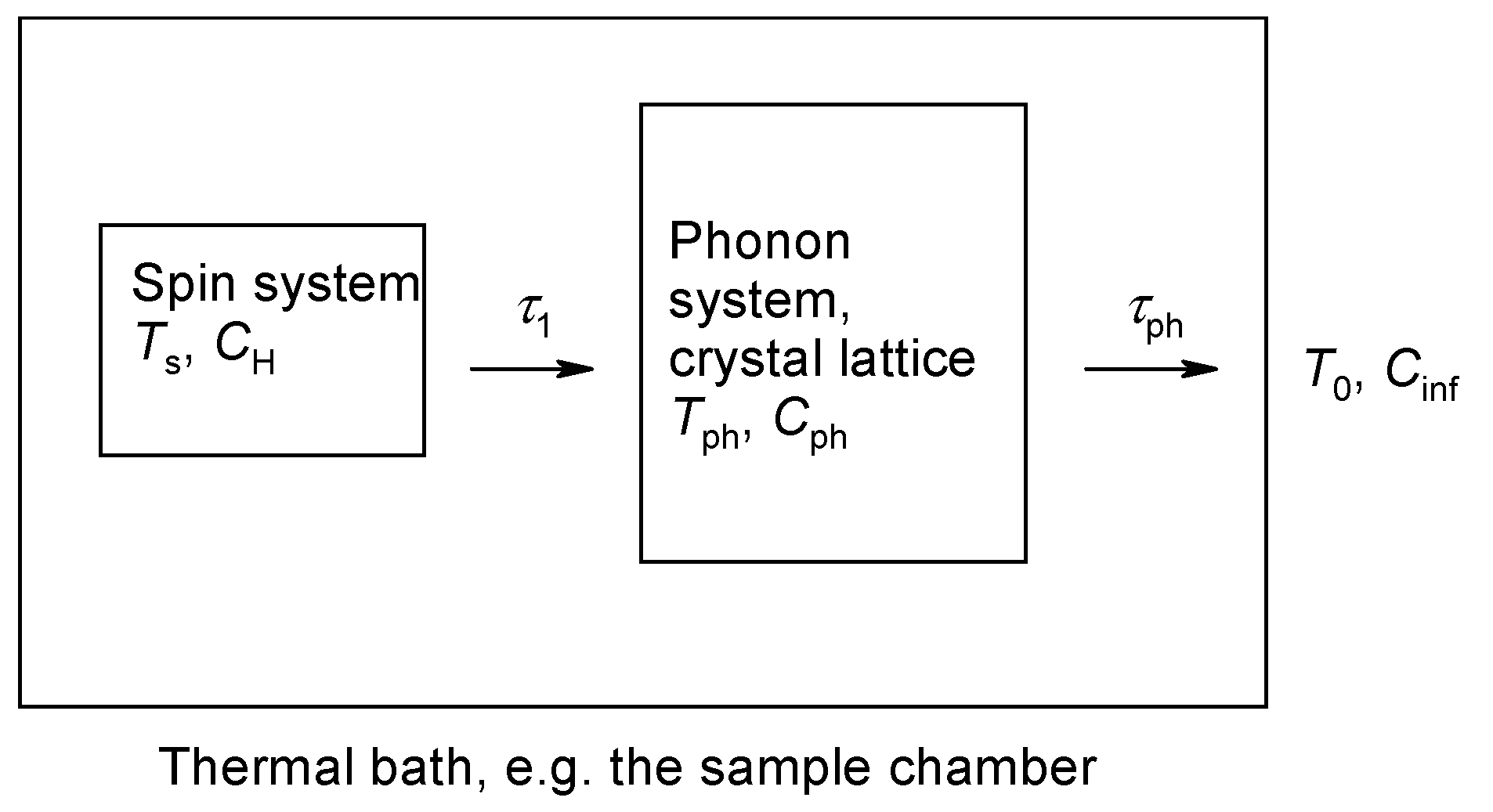
3. Phonon Bottleneck Effect

When analyzing the function lnτ vs. lnT, the low-temperature regime is described by straight lines. The greater the temperature, the lower the relaxation time as follows:

(a)

The Raman process $\ln {\tau }_{\mathrm{Raman}}=-\ln C-n\cdot \ln T$ with n = 5–9;

(b)

The direct process $\ln {\tau }_{\mathrm{direct}}=-\ln A_{\mathrm{dir}}-\ln T$;

(c)

The quantum tunneling process $\ln {\tau }_{\mathrm{qtm}}=-\ln D_{\mathrm{qtm}}$.

Moreover, the function $\ln {\tau }_{\mathrm{Orbach}}=\ln {\tau }_0+(U_{\mathrm{eff}}/k_{\mathrm{B}})\cdot T^{-1}$ referring to the Orbach process is linear in the high-temperature range. This allows an identification of the relaxation process that dominates in a certain temperature interval (Figure 1).

The analysis of experimental data shows that in addition to the above mentioned processes there exists another one for which the equation $\ln \tau =-\ln G-l\cdot \ln T$ or ${\tau }^{-1}=G{T}^l$ is obeyed, but with a subnormal exponent l~2. This indicates a possible presence of the phonon bottleneck effect (note: here we are saying that at a different temperature range a different relaxation “rate” dominates).

The above relaxation mechanisms were based under the assumption that the energy gain given to the phonon system is transferred immediately to the thermal bath of the constant temperature T₀ and a sufficient (infinite) heat capacity. There are, however, two obstacles. (i) The number of spins in a crystal is ca 10²¹ per cm³, whereas the number of available phonon modes at low temperature is significantly lower, by a factor of 10⁶ [18]. (ii) The phonons are scattered on the crystal boundary and some of them are backscattered so that they are not deposited to the thermal bath “just in time”. Owing to this effect, there is some accumulation of the phonons that do not leave the crystal so that apparently the temperature of the phonon bath T_ph is higher than that of the thermal bath: T_ph > T₀. This results in an alteration of the direct relaxation process that is termed the phonon bottleneck effect.

As a result, we can speak about the temperature of the spin system T_s and phonon temperature T_ph. Accordingly, the heat capacity of the spin system (C_H) is greater than that of the phonon (C_ph), i.e., C_H > C_ph (Figure 2).

Based upon arguments about the heat flow, relationships for two relaxation times (time constants) were derived [18] as solutions of the two time-dependent differential equations:

$${\tau }_1^{\prime }={\tau }_1\cdot C_{\mathrm{ph}}/(C_{\mathrm{ph}}+C_H)$$

(3)

$${\tau }_{\mathrm{b}}={\tau }_1+{\tau }_{\mathrm{ph}}\cdot (C_{\mathrm{ph}}+C_H)/C_{\mathrm{ph}}$$

(4)

Notice that τ₁ is the spin to phonon relaxation time and τ_ph is the phonon to thermal bath relaxation time. The relaxation time ${\tau }_1^{\prime }$ is very short, τ_b is slower and it refers to a combined spins + phonons relaxation to the thermal bath.

In a microscopic approach, two differential equations were established [24] giving rise to two time constants ${\tau }_b$ and ${\tau }_b^{\prime }$, hence:

$${\tau }_b={\tau }_{1(\mathrm{direct})}+{\tau }^{\prime }$$

(5)

with

$$\frac{1}{{\tau }^{\prime }}=\frac{1}{{\tau }_{\mathrm{ph}}}\frac{3{\delta }^2(\Delta \delta )}{2{\pi }^{2}c{v}^3{\hslash }^3}{\coth }^2(\delta /2k_{\mathrm{B}}T)\approx \left[\frac{1}{{\tau }_{\mathrm{ph}}}\frac{6(\Delta \delta )k_{\mathrm{B}}^2}{{\pi }^{2}c{v}^3{\hslash }^3}\right]{(T)}^2\to G{T}^2$$

(6)

$$\frac{1}{{\tau }_b^{\prime }}\approx \left[\frac{A{\pi }^{2}c{v}^3{\hslash }^3}{6(\Delta \delta )k_{\mathrm{B}}^2}\right]{(T)}^{-1}\to F{T}^{-1}$$

(7)

Here, c = N/V is the number of spins per cm³ (volume concentration), $\delta =\hslash \omega$ is the ground to excited level separation. In the magnetic field one can use the linewidth $(\Delta \delta )=g{\mu }_{\mathrm{B}}(\Delta B)$. In the role of τ_ph a simple formula can be applied ${\tau }_{\mathrm{ph}}\approx L/2v$ where L is the linear dimension of the crystal and the velocity of sound in the crystal is v~2.5 × 10³ m s⁻¹ (for L = 1 μm, τ_ph~10⁻¹⁰ s [18]). The dependence of the relaxation time upon the crystal size proves that the relaxation is driven by PB [25]. Involvement of the magnetic field modifies the formulae for the relaxation time in the presence of the phonon bottleneck as follows:

$$\frac{1}{{\tau }^{\prime }}\approx C^{\prime }\frac{g(\Delta B)}{{\tau }_{\mathrm{ph}}c}{T}^2\to G_B{T}^2$$

(8)

$$\frac{1}{{\tau }_b^{\prime }}\approx C^{″}\frac{Ac}{(\Delta B)g}{T}^{-1}\to F_B{T}^{-1}$$

(9)

It was argued [24] that the second solution of the phonon bottleneck differential equations ${\tau }_b^{\prime }$ is by several orders of magnitude smaller so that it could be ignored (in diluted ions). To the best of our knowledge, its effect has not been reported until the discovery of the reciprocating thermal behavior in molecular complexes possessing the intermolecular contacts [26].

4. Experimental Part

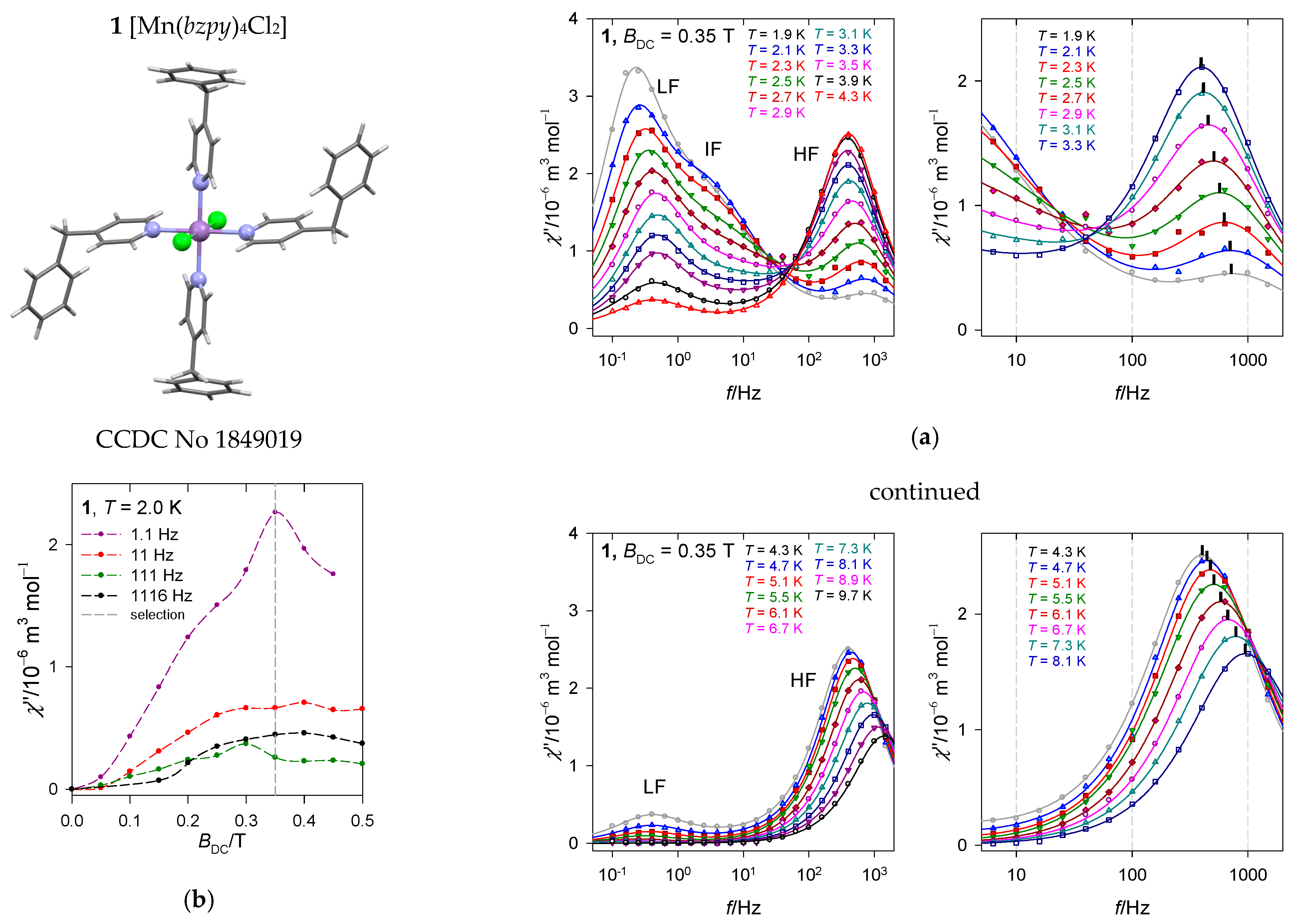
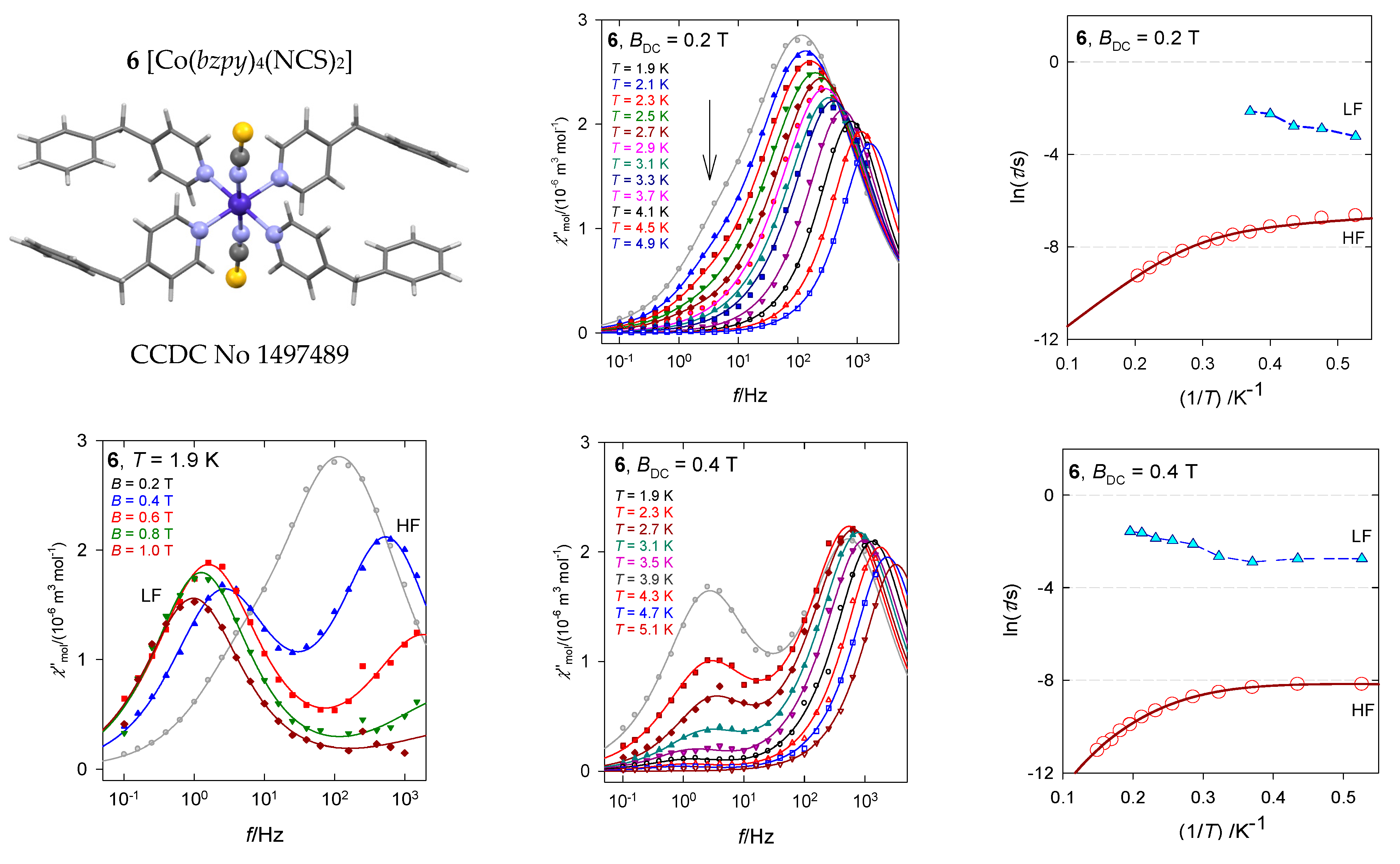
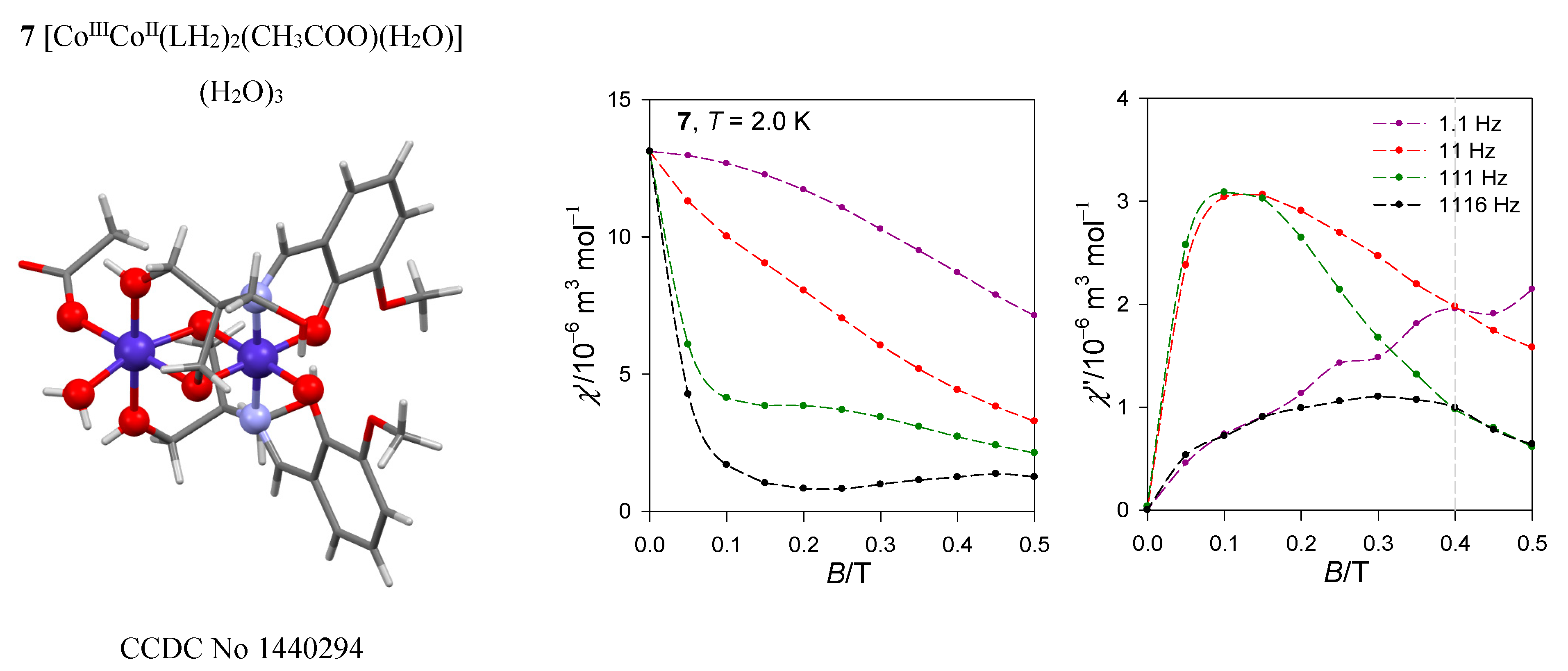
4.1. Synthesis, Chemical Analysis, X-ray Structure, and DC-Magnetic Data

The present communication is a review of the examples where the reciprocating thermal behavior has been detected. The synthetic route and the analytical data can be found in the original publications. The X-ray structure determination has been done in a standard way, preferentially at low temperature, and the principal crystallographic data are deposited in the Cambridge Crystallographic Data Centre. They are available in the “cif” format.

The DC magnetic data were collected with the help of the SQUID apparatus (Quantum Design, MPMS-XL7) restricted to the field B_DC = 7 T and T = 1.8–400 K. Samples in the form of a fine powder were encapsulated in a gelatin sample holder. In DC magnetic experiments, the small field B_DC = 0.1 T has been applied in taking the temperature dependence of the static magnetic susceptibility between T = 1.9–300 K. These data were corrected for the underlying diamagnetism. At the same time, magnetization data were taken until B = 7 T at two temperatures, T = 2.0 and 4.6 K. The DC magnetic data served for the determination of the axial zero-field splitting parameter D; their temperature and/or field dependences were displayed in the published material.

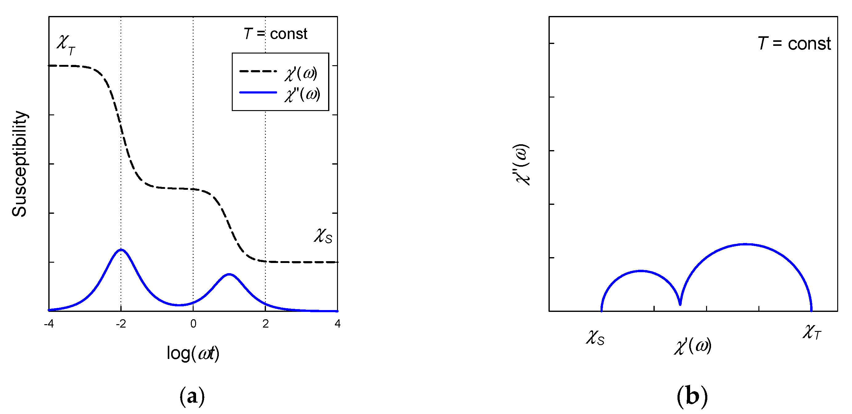
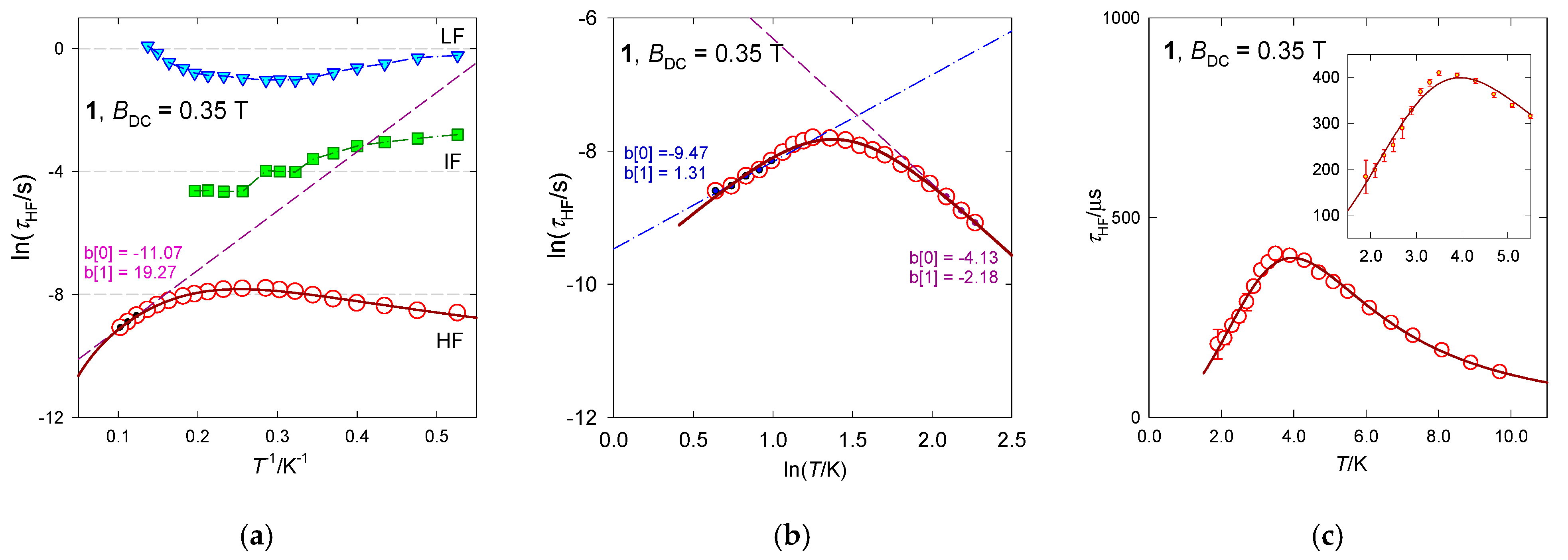
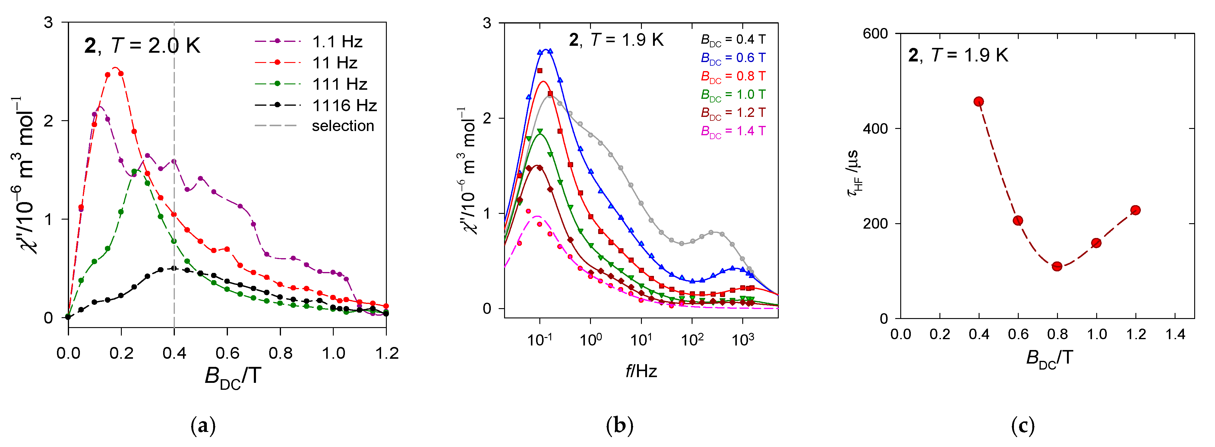
4.2. AC Susceptibility

The AC susceptibility data were taken with the same SQUID apparatus and the same specimen as above using the working amplitude of B_AC = 0.38 mT and frequencies of the oscillating field f = 0.1–1500 Hz.

The first scan refers to a field dependence of the AC susceptibility at the constant low temperature (say T₀ = 2.0 K) for a set of trial frequencies of the oscillating field: f_i = 1.1, 11, 111, and 1111 Hz: ${\chi }^{\prime }=F(B,f_i,[T_0])$ and ${\chi }^{″}=F(B,f_i,[T_0])$. Such graph indicates a field-frequency region where the out-of-phase susceptibility dominates (Figure 3a).

In the second scan, the frequency dependence of the AC susceptibility is monitored for a set of fixed magnetic fields at the constant low temperature ${\chi }^{″}=F(f,B_i,[T_0])$. The frequencies are selected in such a way that the x-axis in the logarithmic scale contains equidistant points. The corresponding graph identifies the number of relaxation channels and their field dependence. The third scan collects the AC response as a function of temperature for the set of frequencies at the fixed external field. This is useful in identifying the critical point where the functions ${\chi }^{\prime }=F(T,f_i,[B_0])$ merge and ${\chi }^{″}=F(T,f_i,[B_0])$ vanishes (Figure 3b). Finally, the displayed function are ${\chi }^{\prime }=F(f,T_i,[B_0])$ and ${\chi }^{″}=F(f,T_i,[B_0])$ that are subjected to the fitting procedure (Figure 3c,d). This dependence is of a primary interest.

The magnetization measured in the oscillating (AC) magnetic fields

$$M_{\mathrm{AC}}=M_0\cos (\omega t-\delta )={\chi }^{\prime }{H}_0\cos (\omega t)+{\chi }^{″}{H}_0\sin (\omega t)$$

(10)

determines the in-phase susceptibility ${\chi }^{\prime }=(M_0/H_0)\cos \delta$ and the out-of-phase component ${\chi }^{″}=(M_0/H_0)\sin \delta$. At low frequencies $\omega =2\pi f$, the delay δ is small so that the out-of-phase component vanishes and the in-phase counterpart approaches the isothermal susceptibility when the magnetic subsystem is in a thermal equilibrium with the lattice subsystem as follows:

$$\underset{\omega \to 0}{\lim }\stackrel{⌢}{\chi }={\left(\frac{\partial M_{\mathrm{AC}}}{\partial H}\right)}_T={\chi }_T$$

(11)

With the increased frequency, the AC susceptibility reaches an opposite limit—adiabatic susceptibility:

$$\underset{\omega \to \infty }{\lim }\stackrel{⌢}{\chi }={\left(\frac{\partial M_{\mathrm{AC}}}{\partial H}\right)}_S={\chi }_S$$

(12)

when $\omega \tau \gg 1$ holds true and the magnetic subsystem is unable to exchange heat with the lattice subsystem and it conserves its entropy. Casimir-DuPré formula [28] connects the isothermal, adiabatic, and AC susceptibilities. After introducing the distribution parameter α, this formula can easily be extended to the multiset form [29] as follows:

$$\chi (\omega )={\chi }_S+{\displaystyle \sum _k^K\frac{{\chi }_k-{\chi }_{k-1}}{1+{(\mathrm{i}\omega {\tau }_k)}^{1-{\alpha }_k}}}$$

(13)

The in-phase and out-of-phase components can be written in closed forms which in the case of a two-set model are [29] as follows:

$$\begin{array}{c}{\chi }^{\prime }(\omega )={\chi }_S+({\chi }_{T1}-{\chi }_S)\frac{1+{(\omega {\tau }_1)}^{1-{\alpha }_1}\sin (\pi {\alpha }_1/2)}{1+2{(\omega {\tau }_1)}^{1-{\alpha }_1}\sin (\pi {\alpha }_1/2)+{(\omega {\tau }_1)}^{2-2{\alpha }_1}}\\ +({\chi }_{T2}-{\chi }_{T1})\frac{1+{(\omega {\tau }_2)}^{1-{\alpha }_2}\sin (\pi {\alpha }_2/2)}{1+2{(\omega {\tau }_2)}^{1-{\alpha }_2}\sin (\pi {\alpha }_2/2)+{(\omega {\tau }_2)}^{2-2{\alpha }_2}}\end{array}$$

(14)

$$\begin{array}{c}{\chi }^{″}(\omega )=({\chi }_{T1}-{\chi }_S)\frac{{(\omega {\tau }_1)}^{1-{\alpha }_1}\cos (\pi {\alpha }_1/2)}{1+2{(\omega {\tau }_1)}^{1-{\alpha }_1}\sin (\pi {\alpha }_1/2)+{(\omega {\tau }_1)}^{2-2{\alpha }_1}}\\ +({\chi }_{T2}-{\chi }_{T1})\frac{{(\omega {\tau }_2)}^{1-{\alpha }_2}\cos (\pi {\alpha }_2/2)}{1+2{(\omega {\tau }_2)}^{1-{\alpha }_2}\sin (\pi {\alpha }_2/2)+{(\omega {\tau }_2)}^{2-2{\alpha }_2}}\end{array}$$

(15)

Here, the isothermal and adiabatic susceptibilities are constrained as ${\chi }_S<{\chi }_{T1}<{\chi }_{T2}$ in order to get positive contributions from each primitive component. The above formula can be rewritten using the mole fractions of the respective k-components x_k

$$\chi (\omega )={\chi }_S+({\chi }_T-{\chi }_S)\left[\frac{x_1}{1+{(\mathrm{i}\omega {\tau }_1)}^{1-{\alpha }_1}}+\frac{x_2}{1+{(\mathrm{i}\omega {\tau }_2)}^{1-{\alpha }_2}}\right], x_2=1-x_1$$

(16)

that fulfil $x_1=({\chi }_{T1}-{\chi }_S)/({\chi }_T-{\chi }_S)$ and $x_2=({\chi }_{T2}-{\chi }_{T1})/({\chi }_T-{\chi }_S)$.

A plot of ${\chi }^{″}$ vs. ${\chi }^{\prime }$ at the constant temperature refers to the Argand diagram (analogous to the Cole-Cole diagram for dielectrics). In an ideal case, it is a semicircle providing that there is a single relaxation time. The distribution parameter α causes its distortion to an arc. In the case of a two-set model two arcs are overlapping (Figure 4).

5. Theoretical Part

5.1. Spin Hamiltonian

The simplest theoretical model used in interpreting magnetic data (magnetization, DC-susceptibility, electron spin resonance) is based upon the spin-Hamiltonian formalism. This method utilizes a formal Hamiltonian containing the spin-only operators acting on the basis set of spin-only kets $|S,M_S\rangle$. One particular form refers to the zero-field splitting

$$\begin{array}{ll}{\widehat{H}}_{kl}^{\mathrm{zfs}}=& D({\widehat{S}}_z^2-{\overrightarrow{S}}^2/3){\hslash }^{-2}+E({\widehat{S}}_x^2-{\widehat{S}}_y^2){\hslash }^{-2}\\ & +{\mu }_{\mathrm{B}}B(g_z{\widehat{S}}_z\cos {\vartheta }_k+g_x{\widehat{S}}_x\sin {\vartheta }_k\cos {\phi }_l+g_y{\widehat{S}}_y\sin {\vartheta }_k\sin {\phi }_l){\hslash }^{-1}\end{array}$$

(17)

where the axial (rhombic) zero-field splitting parameters D (E) occur. The Zeeman term involves the spin operators and the magnetic field oriented towards grids is uniformly distributed over a sphere ($\vartheta$ and $\phi$ are polar angles). Frequently, simplifications are applied, such as consideration of only Cartesian components. An ultimate demand is that the ground electronic term is non-degenerate (A- or B-type) and well separated from the excited electronic terms. For tetrahedral Co(II) with the ⁴A₂ ground term, there are only four kets $|3/2,\pm 1/2\rangle$ and $|3/2,\pm 3/2\rangle$ forming two Kramers doublets [30].

5.2. Griffith-Figgis Model

The energy levels of hexacoordinate Co(II) complexes are derived from the octahedral mother term ⁴T_1g that bears the non-zero orbital angular momentum L. The situation describes the spin-orbit Hamiltonian which works in the space of the spin- and orbital- kets $|L=1,M_L,S,M_S\rangle$ as outlined by Griffith and extended by Figgis (hereafter the GF model).

$$\begin{array}{ll}{\widehat{H}}^{\mathrm{GF}}=& -(A\kappa \lambda )({\overrightarrow{L}}_{\mathrm{p}}\cdot \overrightarrow{S}){\hslash }^{-2}+{\mathsf{\Delta }}_{\mathrm{ax}}({\widehat{L}}_{\mathrm{p},z}^2-{\overrightarrow{L}}_{\mathrm{p}}^2/3){\hslash }^{-2}+{\mathsf{\Delta }}_{\mathrm{rh}}({\widehat{L}}_{\mathrm{p},x}^2-{\widehat{L}}_{\mathrm{p},y}^2){\hslash }^{-2}\\ & +{\mu }_{\mathrm{B}}{g}_{\mathrm{e}}(\overrightarrow{B}\cdot \overrightarrow{S}){\hslash }^{-1}-{\mu }_{\mathrm{B}}(A\kappa )(\overrightarrow{B}\cdot {\overrightarrow{L}}_{\mathrm{p}}){\hslash }^{-1}\end{array}$$

(18)

The spin-orbit coupling involves the free-ion spin-orbit splitting parameter λ = −ξ/2S, the orbital and spin Zeeman terms, and the axial (rhombic) crystal-field splitting parameter Δ_ax (Δ_rh). In addition, ξ is the spin-orbit coupling constant and the other symbols are in their usual meaning. The remaining parameters involve the orbital reduction factor κ, and the Figgis CI parameter A. Due to the T-p isomorphism the orbital angular momentum is L_p = 1 and g_L = −1. This Hamiltonian can be treated by a numerical procedure. For Co(II), λ/hc = −155 cm⁻¹ and the spin-orbit kets cover 12 multiplets forming six Kramers doublets belonging to the irreducible representations of the respective double group [30].

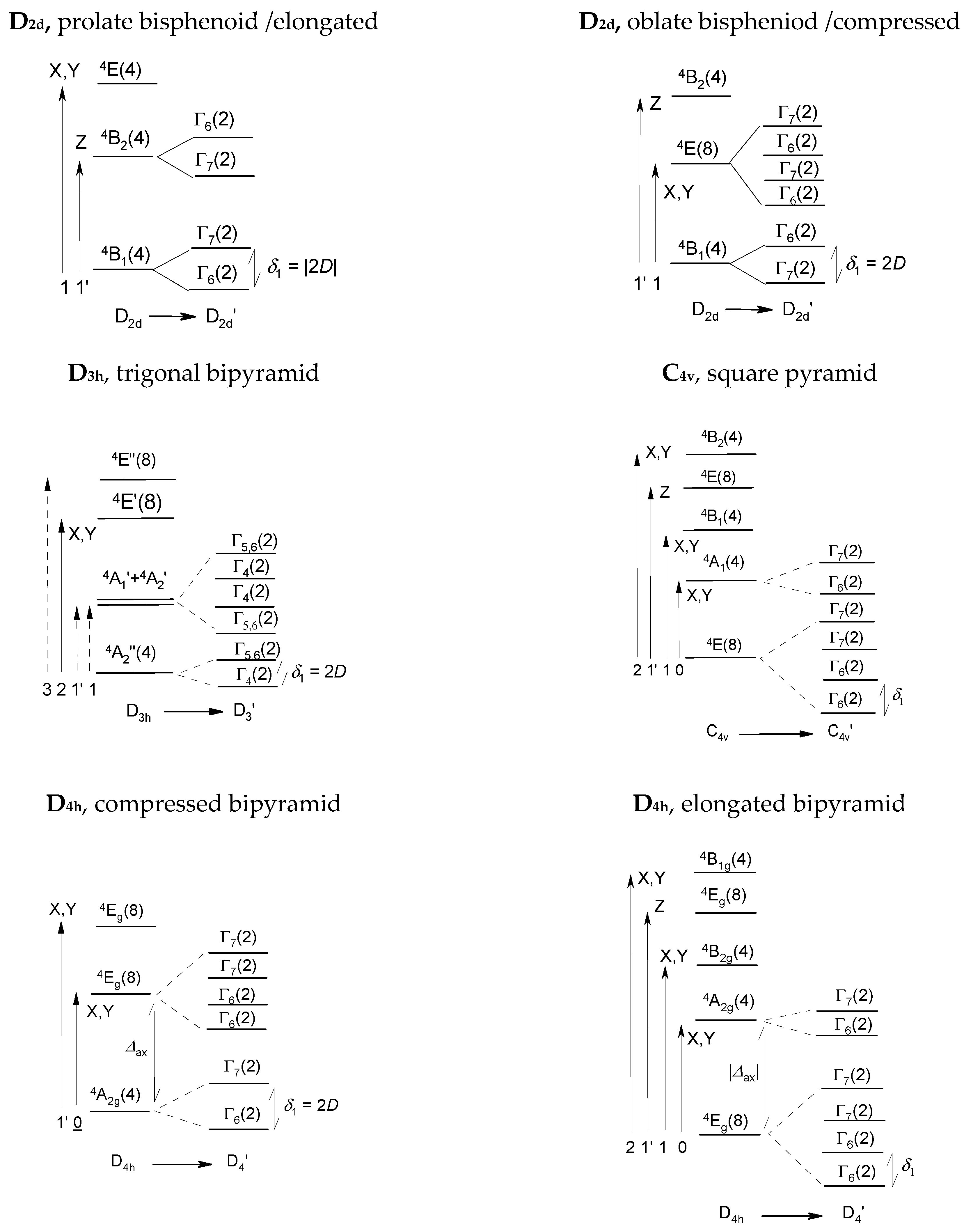
5.3. Crystal Field Calculations

The generalized crystal-field method is working in the complete set of kets generated by the dⁿ configuration (e.g., 120 for Co(II)). By involving the electron repulsion, crystal-field potential, spin-orbit, orbital and spin Zeeman terms a detailed evaluation of the electronic levels (crystal-field multiplets and Zeeman levels) can be done in a short time. The internal parameters of the method are the crystal field poles F₄(L) and eventually F₂(L) for each ligand, the Racah parameters of the interelectron repulsion B and C, and the spin-orbit coupling constant ξ. The crystal-field pole strength $F_k(R_L)=R_L^{-(k+1)}\langle r^k\rangle$ of k-th power for the ligand L situated at the distance R_L involves the momentum integral over the electronic variables $\langle r^k\rangle$. It relates to the common ligand field strength, e.g., $10Dq=(10/6)F_4(R_L)$ for an octahedral system. Consequently, the spin-Hamiltonian parameters D, E, g_z, g_x, g_y, χ_TIP can be evaluated [31].

5.4. Ab Initio Calculations

Contemporary ab initio calculations start with the CASSCF module with inclusion of the relativistic effects followed by the NEVPT2 block that involves the spin-orbit interaction [32]. Spin-orbit corrected energy levels refer to the crystal-field multiplets and in the case of Co(II) systems to the set of Kramers doublets. The spin Hamiltonian parameters can be evaluated in the case of the orbitally non-degenerate ground electronic term. If the algorithm is applied to the case of the (quasi) degenerate ground term, the results can be false. Useful results can be obtained only by considering a large and flexible basis set for the involved atoms.

SH, GF, and ORCA/SO splitting are completely different tasks. For Co(II) systems, SH considers only two Kramers doublets arising from the ⁴A₂ ground term split by δ. GF considers six Kramers doublets arising from the ⁴T_1g term on symmetry lowering (only in the case of the compressed tetragonal bipyramid δ is comparable with the SH value). Ab initio ORCA/SO calculations reproduce the complete energy spectrum and thus are superior.

5.5. Fitting Procedures

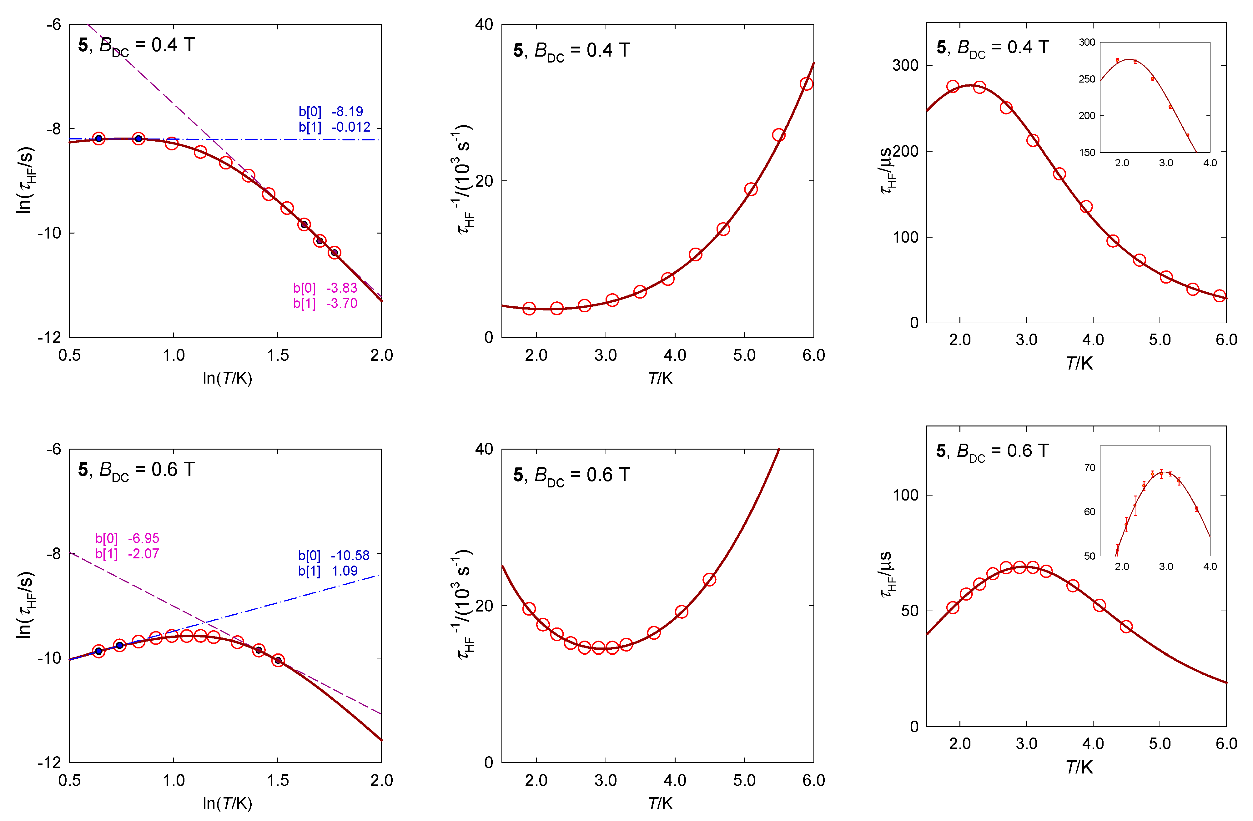
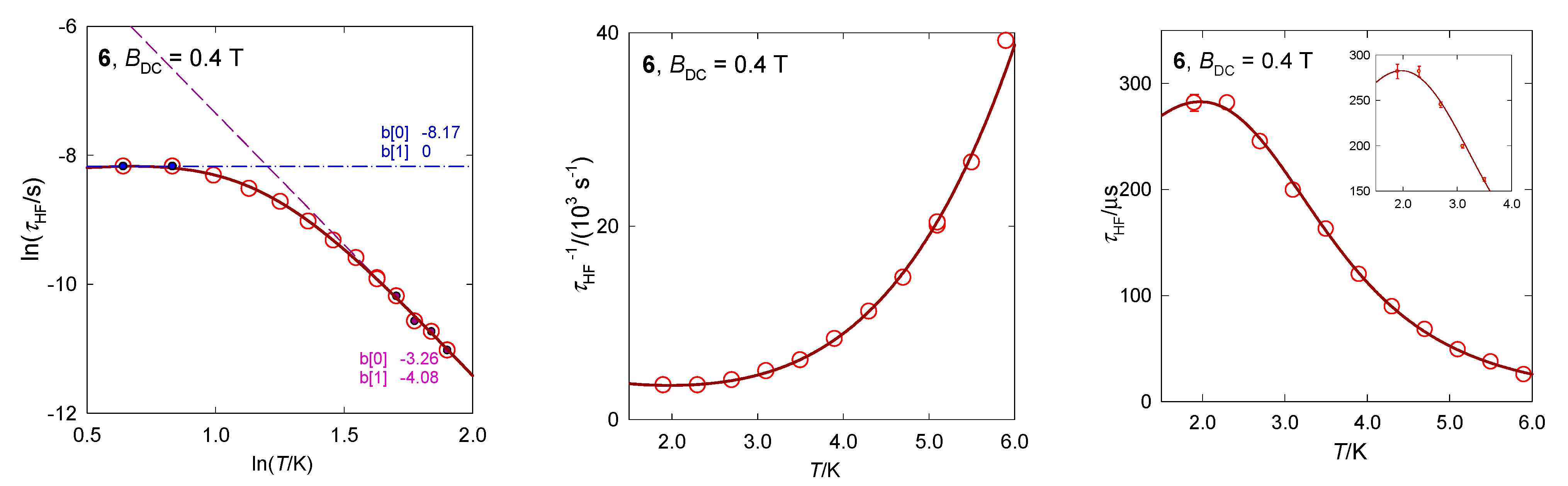
For temperature evolution of the molar magnetic susceptibility of Co(II) systems, some closed formulae can be found in the literature (see, for instance [30,31]). These, however, do not reproduce a correct powder average and they are missing for the field dependence of the magnetization.

Having energy levels at the disposal by the diagonalization of the model Hamiltonian in the given basis set, one can proceed by applying methods of statistical thermodynamics. For the given DC field, the partition function is formed $Z_{kl}(T,B)$ and its derivatives yield the magnetization $M_{kl}(T,B)$ and susceptibility ${\chi }_{kl}(T,B)$ referring to the grids of the magnetic field in Zeeman term. Then, an average produces the magnetic functions that match the powder nature of the sample.

Since the DC-susceptibility and DC-magnetization both reflect the same electronic structure of the sample, their fitting can be done simultaneously by minimizing a properly chosen error function. This is $F=w\cdot E(\chi )+(1-w)\cdot E(M)$ or $F=E(\chi )\cdot E(M)$ with the weight w, $E(\chi )$, and $E(M)$ representing the relative errors of the susceptibility and magnetization, respectively.

An analogous procedure can be utilized for a simultaneous fitting of the in-phase and out-of-phase components of the AC susceptibility: $F=w\cdot E({\chi }^{\prime })+(1-w)\cdot E({\chi }^{″})$. Here, $E({\chi }^{\prime })$ and $E({\chi }^{″})$ are relative errors of the components when using the one-set, two-set or three-set Debye model. Since there are simple closed formulas for them, no problem is found to apply several hundred-thousand searches for advanced non-linear optimization algorithms such as genetic algorithms.

The primitive functions of the Debye model possess a useful property: The peak of χ″ is perfectly symmetric with respect to log f. Figure 5 visualizes a test of the stability of the fitting procedure when the experimental points are reduced from the right side—high frequencies. An omission of 1 through 7 data points has a negligible effect to the fitted set of seven parameters even in the difficult case when the LF channel appears as a shoulder. The graph is a superposition of eight lines, each fitted independently. This finding approves the determination of the relaxation parameters even in the case when the data taking is stopped (not allowed by the hardware, e.g., f < 1500 Hz) before reaching the peak maximum. However, one has carefully checked the standard deviations of the parameters and eventually their pair-correlation (see Supplementary Information). The advantage of the fitting procedure lies in the fact that it can separate the primitive components also in the case of their overlap (resulting in a shoulder).

6. Data Analysis

6.1. DC Magnetic Data

For a series of tetra-, penta-, and hexacoordinate Co(II) complexes, the values of the axial zero-field splitting parameter D extracted from the magnetic data are listed in

Table 2. Comparison of selected Co(II) complexes showing SMR.

Complex	No.	SMR a	RTB b	Channels c	Jd	D(MS&M) e	D(Ab Initio) e	Ref.
Hexa-coordination
[Co(pydca)(dmpy)]·0.5H2O	2	Y	Y	3		55	(−67.2) (−121)	[26]
[Co(bzpy)4Cl2]	5	Y	Y	3		106	88.6 124	[34]
[Co(bzpy)4(NCS)2]	6	Y	Y	2		90.5	88.6 90.8	[34]
[CoIIICoII(H2L)2(ac) (H2O)] (H2O)3	7	Y	Y	2		(145)	(−99.6)	[35]
[Co(dmpy)2](dnbz)2		Y		3		(43.6)	(−94.8)	[27]
[Co(dppmO,O)3] [Co(NCS)4]		N	-	-		O 83, T −5.0	O 102, T −3.5	[36]
[Co(dppmO,O)3] [CoCl4]		Y	N	2		O 77, T 4.6	O 157, T −1.9	[36]
[Co(dppmO,O)3] [CoBr4]		Y	N	2		O 122, T 15.0	O 129, T −2.5, T 6.6	[36,37]
[Co(dppmO,O)3] [CoI4]		Y	N	2		O 99, T 19.3	O 107, T 14.9	[36]
Penta-coordination
[Co(Me6tren)Cl]ClO4, sim		Y		2		−4.9, −6.2	−9.73, epr −8.12	[38,39]
[Co(Me6tren)Br]Br		Y		na		−2.5	−2.12, epr −2.40	[39]
[Co(bzimpy)Cl2]·DMF	8	Y		2		58.4	(−87)	[40]
[Co(bzimpy)Br2]·DMF	9	Y	Y	2		47.0	63.7	[40]
[Co(bzimpy)I2]		Y		2		40.0		[40]
[Co(LI)Cl2]		Y		2		61.9	(−62)	[41]
[Co(LC7)Cl2]		Y		2	1.54	153	(−119)	[41]
[Co(LC10)Cl2]		Y		2	1.42	70.1	44.2	[41]
[Co(LC12)Cl2]		Y		2		46.8	43.4	[41]
[Co(LC14)Cl2]		Y		2	1.06	87.5	(−58)	[41]
[(N3)2CoIII(L)(μ-N3)CoII(N3)]·2MeOH		Y		2		38.7	42.4	[42]
Tetra-coordination
[Co(PPh3)2(NCS)2]		Y		2		−9.44	−12.2	[43]
[Co(DPEphos)Cl2]		Y		1			−14.4	[44]
[Co(Xantphos)Cl2]		Y		1			−15.4	[44]
[Co(PPh3)2Cl2]		Y		1 (2)		−11.6	−16.2, epr −14.8	[44,45,46]
[Co(PPh3)2Br2]	10	Y	Y	2		−12.5		[47]
[Co(PPh3)2I2]		Y		1		−36.9		[48]
[Co(AsPh3)2I2]		Y		1		−74.7		[48]
[Co(qu)2I2]		N		−		9.2		[48]
[Co(bcp)Cl2]		Y		1	0.24	−6.62		[49]
[Co(bcp)Br2]		N		−	−0.023	−6.72		[49]
[Co(bcp)I2]		N		−	−0.63	−7.03		[49]
[Co(dmphen)Br2]		Y		2		10.6	epr 11.7	[50]
[Co(dmphen)Cl2]		N		−	−1.00	11.9	15.6	[51]
[Co(dmphen)Br2]		N		2, 3		13.8	13.8	[51]
[Co(dmphen)I2]		Y		2, 3		16.6	11.4	[51]
[Co(biq)Cl2]	11	Y	Y	2		10.5	16.1	[33]
[Co(biq)Br2]		Y		2		12.5	14.7	[33]
[Co(biq)I2]		Y		2		10.3	13.7	[33]

^a SMR—slow magnetic relaxation. Bold—true single ion magnets in the zero field. ^b RTB—reciprocating thermal behavior. Blank field means that the reciprocating thermal behavior has not been detected in the applied DC fields. ^c Number of relaxation channels (modes) in the applied DC field. ^d J—isotropic exchange coupling constants in cm⁻¹ conforming convention –J in the spin Hamiltonian. ^e D(MS&M)—axial zero-field splitting parameter extracted from the magnetic susceptibility and magnetization; D(ab initio) from calculations, eventually from epr (electron paramagnetic resonance) in units of cm⁻¹. Values in brackets could be false due to the orbitally (quasi) degenerate electronic ground term and a divergence of the perturbation theory.

along with available ab initio data using the CASSCF + NEVTP2 method (ORCA package). The high-frequency/high-field EPR data are also quoted when available.

For tetracoordinate Co(II) complexes, in geometry of a compressed and also elongated bisphenoid, the ground electronic term is orbitally nondegenerate ⁴A₂ (Figure 6). This justifies an application of the spin Hamiltonian formalism and the experimental data on D reasonably match theoretical predictions. The majority of these systems exhibit slow magnetic relaxation (SMR) with 1, 2 or 3 relaxation channels irrespective of the sign of the D-parameter (Orbach relaxation mechanism requires negative D values). In certain cases, however, the exchange interaction of the antiferromagnetic nature prevents the observation of SMR.

For the hexacoordinate Co(II) system the electronic terms are daughters of the octahedral ⁴T_1g that is orbitally triply degenerate. On a tetragonal compression the daughter ground term is orbitally non-degenerate ⁴A_1g for which the spin-Hamiltonian formalism is legitimate to apply. The D-parameter adopts high positive values, D/hc~100 cm⁻¹, and separates two Kramers doublets [30,31]. The positive D-value discriminates the presence of the Orbach mechanism since now the barrier to spin reversal, requiring D < 0, does not exist.

On a tetragonal elongation the ground daughter term stays doubly degenerate ⁴E_g and the spin-Hamiltonian formalism cannot be applied. Eight magnetic levels forming four Kramers doublets are in the play. Consequently, the D-parameter is undefined. When the ab initio calculations of the spin-Hamiltonian parameters are, as program options, activated, the results could be false (e.g., D < 0, g_z < 2). Moreover, in the case of quasi degeneracy the ab initio predictions could fail due to the divergence of the perturbation theory. The same obstacles hold true for the pentacoordinate Co(II) complexes in the geometry of the square pyramid.

A few complexes reviewed in Table 2, in addition to the SMR (SIM) behavior, show the reciprocating thermal behavior (RTB) referring to the high-frequency channel of the slow magnetic relaxation. These are collected in

Table 3. Characteristics of the reciprocating thermal behavior for high-frequency channel of slow magnetic relaxation in transition metal complexes ^a.

No.	Chromophore	BDC/T	G /K−l s−1 C /K−n s−1	l or n	F /Kk s−1	k	Ref.
1 [Mn(bzpy)4Cl2]	MnN4Cl2	0.35	57(13)	2.20(10)	20.1(2)	1.98(12)	[52]
2 [Co(pydca)(dmpy)]·0.5H2O	CoN2O4	0.40	0.13(1)	5.93(4)	3.7(1) × 103	0.78(3)	[26]
3 [Cu(pydca)(dmpy)]·0.5H2O	CuN2O4	0.5	46(13)	1.9(1)	2.5(4) × 103	0.73(18)	[53]
		1.0	5.6(42)	2.6(3)	4.2(6) × 103	0.79(17)
4 [Ni(pydca)(dmpy)]·H2O	NiN2O4	0.4	10.3(2)	4.7	3.4(1) × 103	0.58	[54]
		0.6	6.4(3)	4.76	8.0(3) × 103	0.84
5 [Co(bzpy)4Cl2]	CoN4Cl4	0.4	19(5)	4.17(16)	5.1(7) × 103	0.63(19)	[34]
		0.6	68(19)	3.66(18)	40.9(17) × 103	1.22(7)
6 [Co(bzpy)4(NCS)2]	CoN4N2	0.4	18(5)	4.26(14)	4.3(6) × 103	0.42(22)	[34]
7 [CoIIICoII(LH2)2(ac)(H2O)] (H2O)3	CoO4OO	0.4	33(9)	4.10(14)	9.1(12) × 103	0.75(19)	[35]
8 [Co(bzimpy)Cl2]·DMF	CoN3Cl2	0.4	3.4(8)	5.36(14)	7.3(1) × 103	[0]	[40]
9 [Co(bzimpy)Br2]·DMF	CoN3Br2	0.2	48(19)	4.00(25)	10.2(12) × 103	0.75(21)	[40]
	CoN3Br2	0.4	12.1(45)	5.08(24)	28(1) × 103	0.56(6)
10 [Co(PPh3)2Br2]	CoP2Br2	0.2	0.098(82)	12.4(8)	67(18)	2.53(41)	[47]
11 [Co(biq)Cl2]	CoN2Cl2	0.3	0.0083(17)	12.0(2)	2.3(4) × 103	1.0(3)	[33]

^a Equation ${\tau }^{-1}=G{T}^l+F{T}^{-k}$ or ${\tau }^{-1}=C{T}^n+F{T}^{-k}$. Standard deviations in parentheses. Resulting parameters of the non-linear fitting for the whole temperature range can be slightly different from those referring to the linear fits to a limited temperature point.

along with fitted parameters that reproduce a temperature development of the high-frequency relaxation time using a simple equation ${\tau }^{-1}=G{T}^l+F{T}^{-k}$. There is one obstacle: When the parameters G and l (F and k) are allowed to float, they could be mutually dependent: With the increasing G the parameter l decreases and vice versa. This may have a minor influence for the interpolated data, but sometimes brings a wrong prediction in extrapolation. Therefore, also the correlation coefficients ρ(G, l) and ρ(F, k) need be monitored.

The extensive graphs reported below show the experimental points of the out-of-phase susceptibility as a function of the frequency of the oscillating magnetic field and/or applied DC field. The high-temperature tail of the data was analyzed by employing the linear regime for the lnτ vs. T⁻¹ dependence written as lnτ = b[0] + b[1]·T⁻¹. The tangential b[1] refers not necessarily to the Orbach process (effective barrier to the spin reversal) since the possible limits are in the data taking/analysis. The intermediate/low temperature regime was analyzed using the lnτ vs. lnT function (see Figure 1).

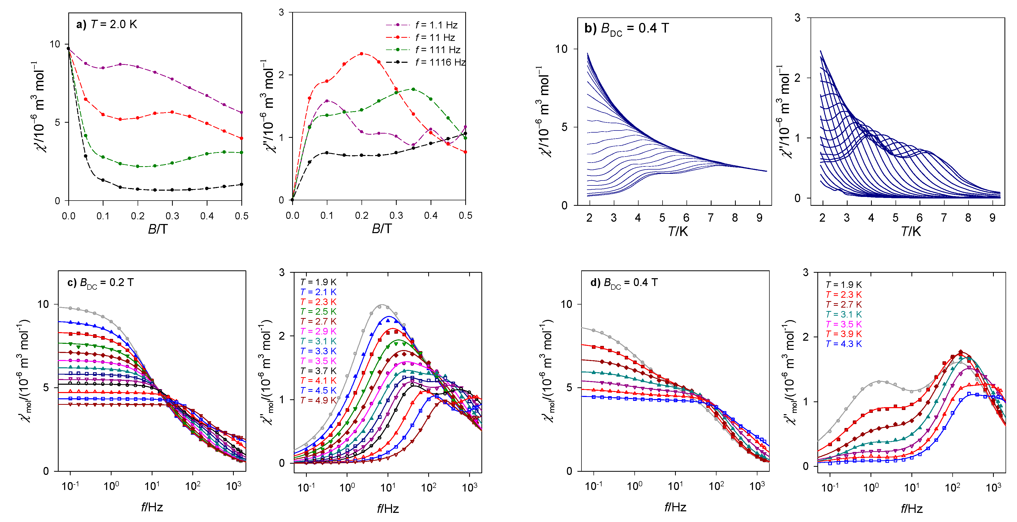
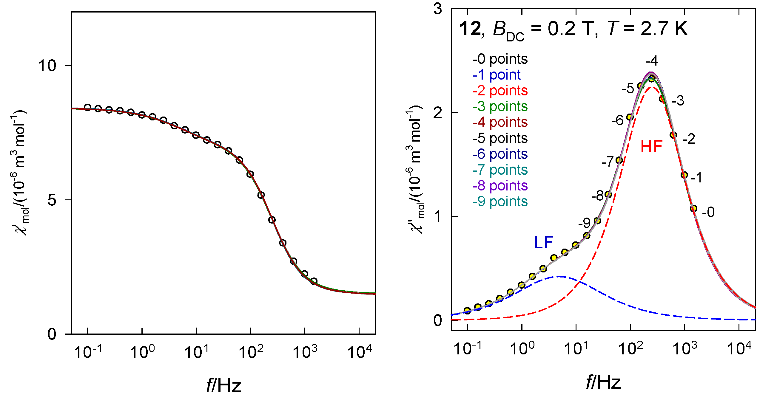
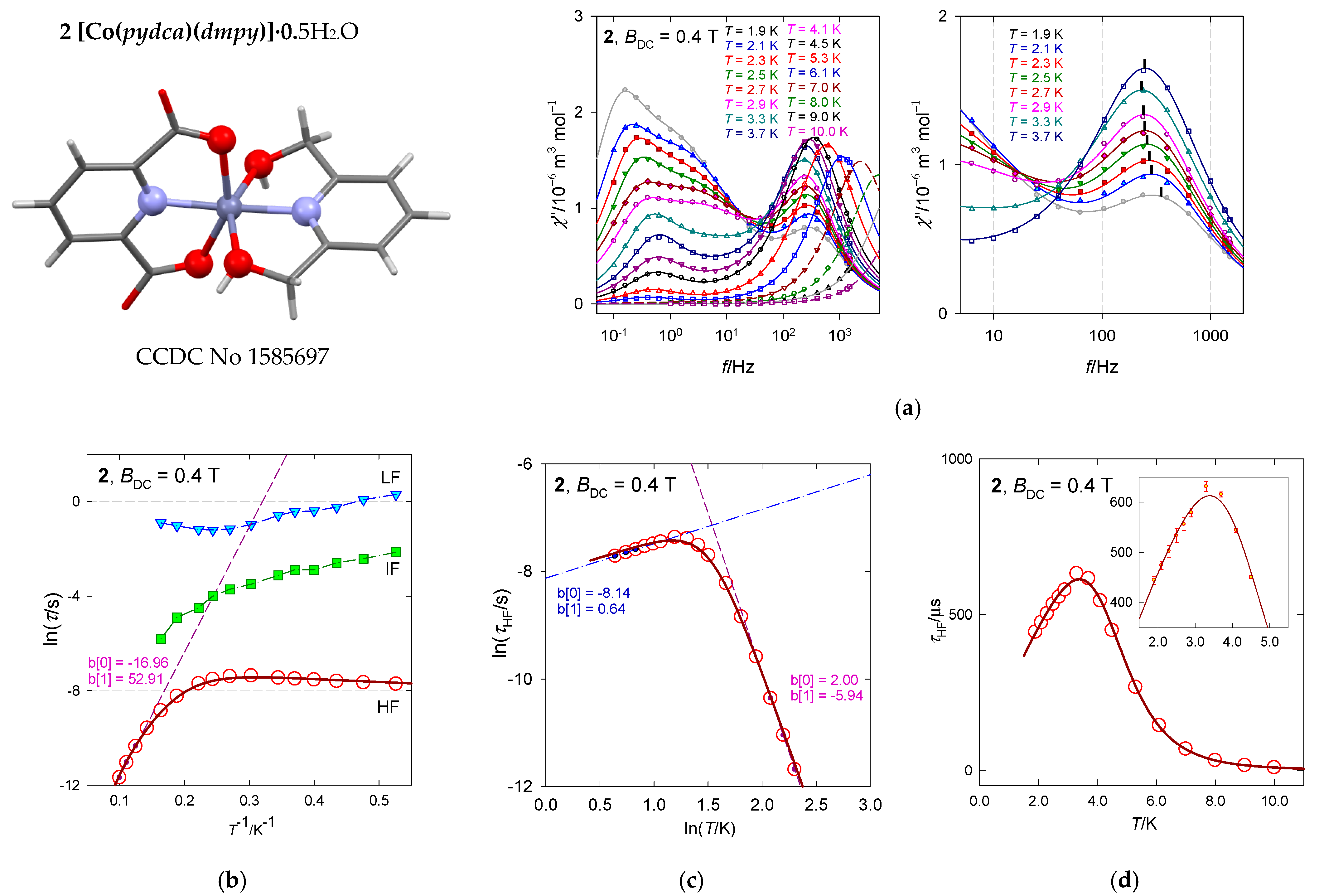
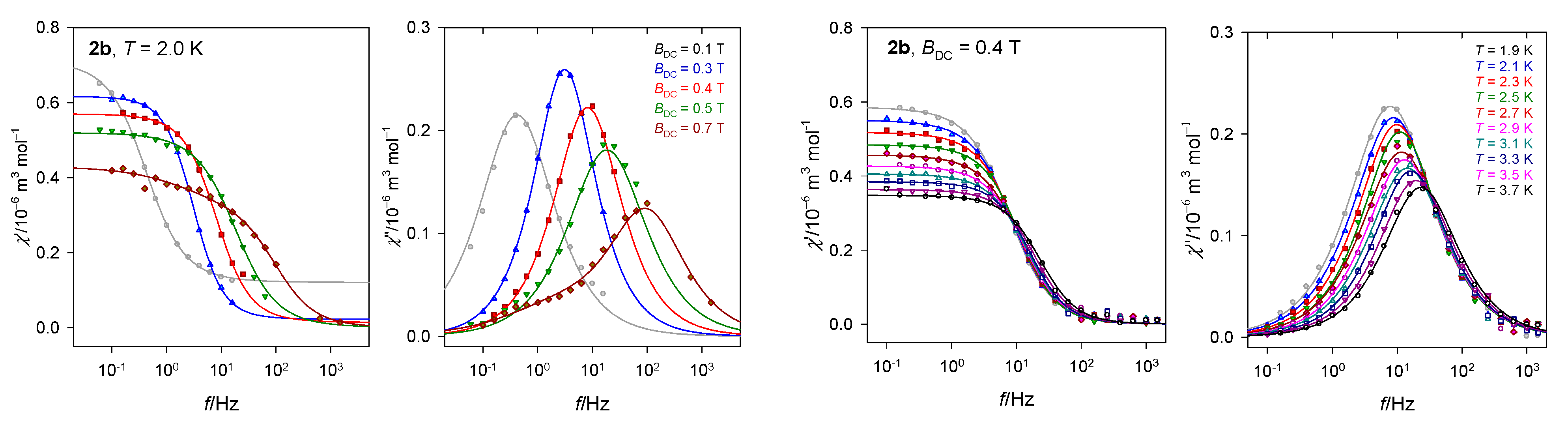
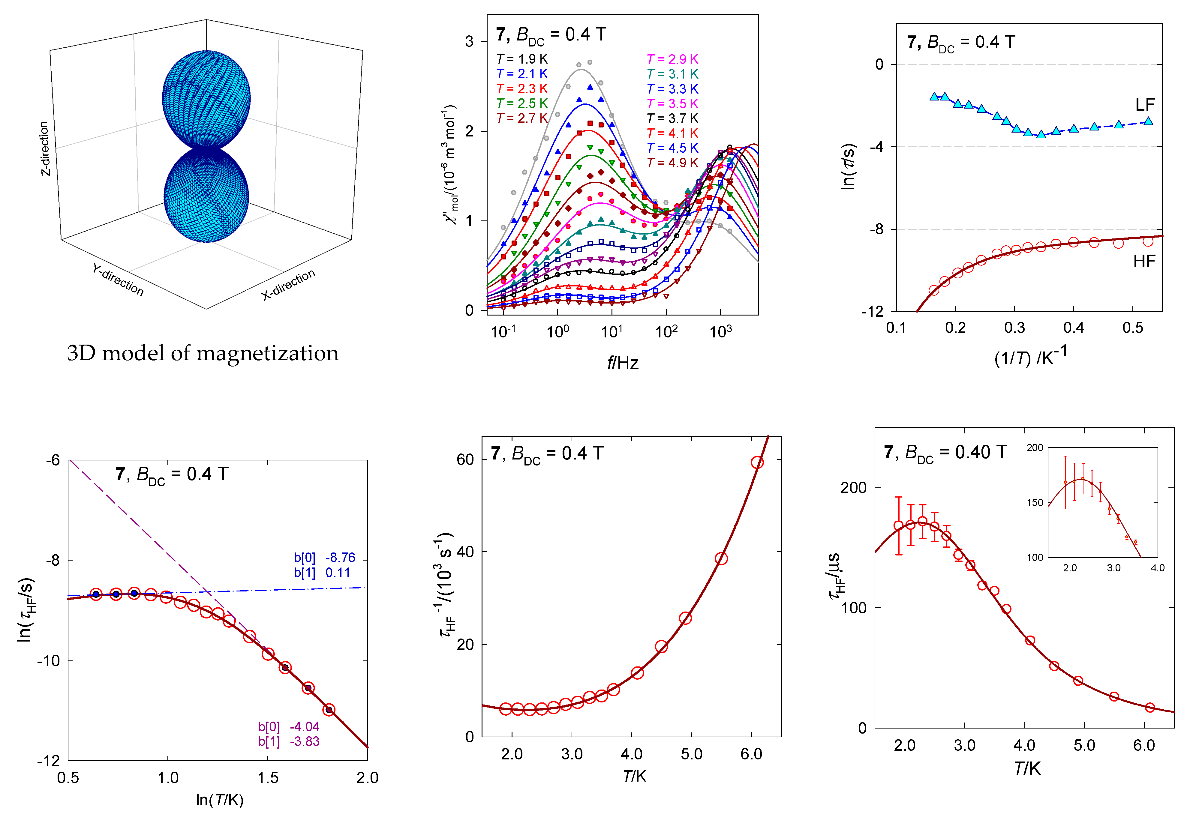
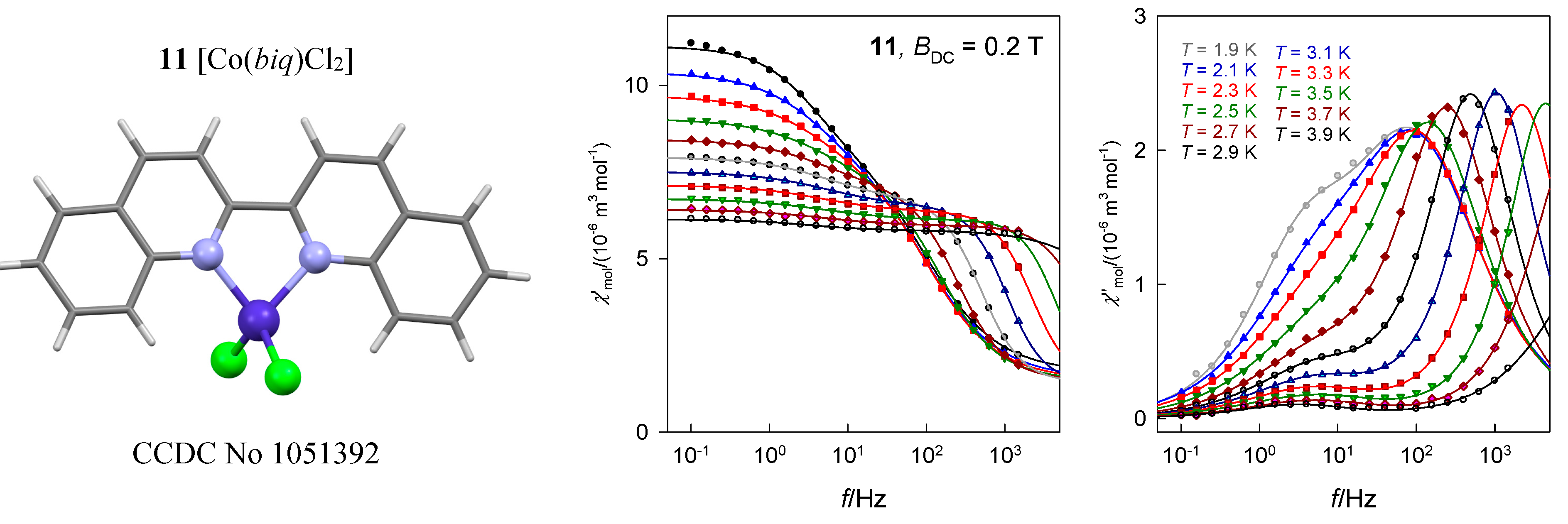
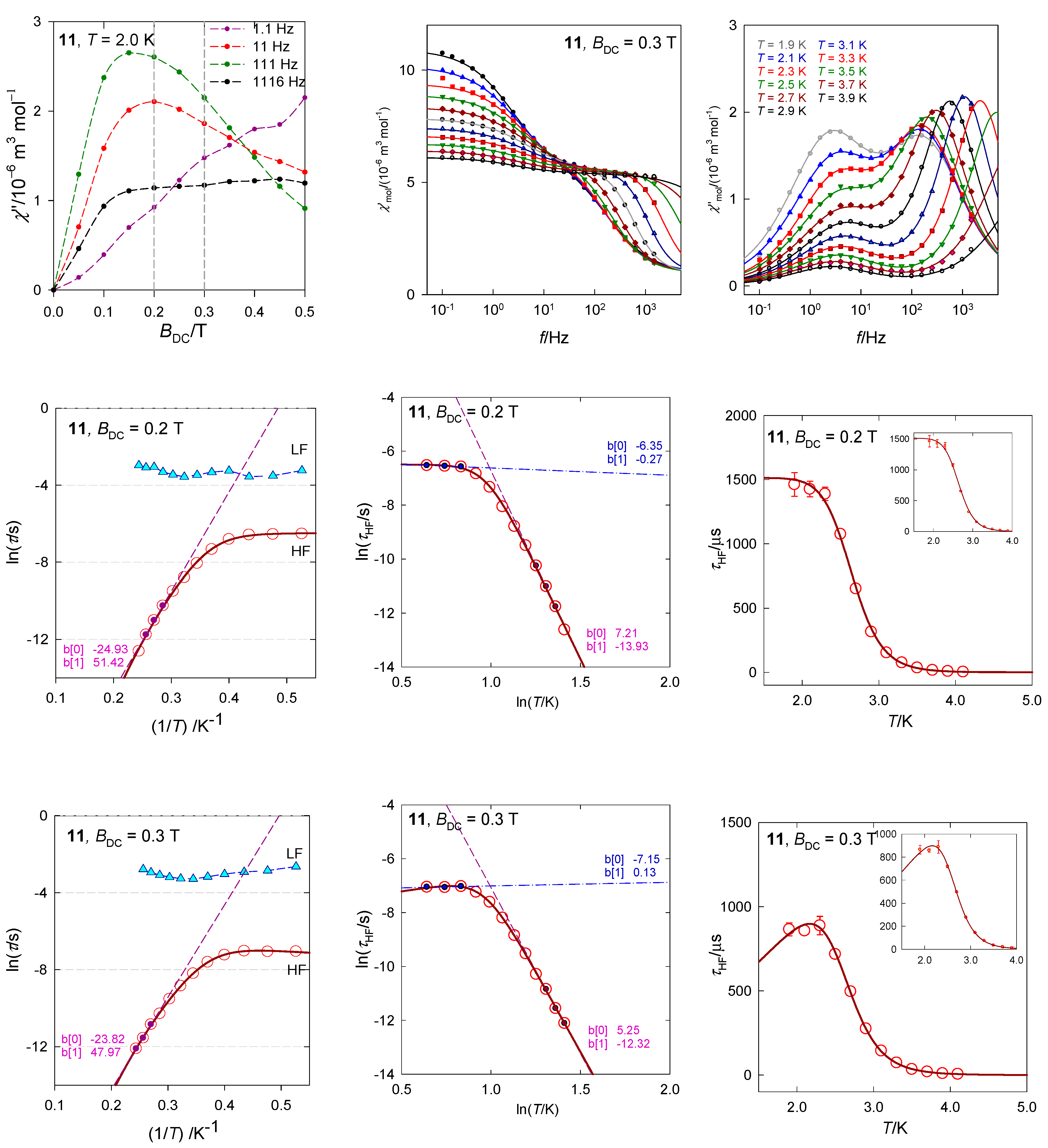
6.2. Example of Reciprocating Thermal Behavior

The hexacoordinate complex [Mn^II(bzpy)₄Cl₂], hereafter 1, belongs to the class of SIMs showing RTB [52]. This S = 5/2 spin system with ⁶A_1g ground electronic term possesses a very low (rather negligible) D-parameter as verified by the DC magnetic data and ab initio calculations: D/hc = −0.63 cm⁻¹. A small D-value is also indicated by simulation of the X-band EPR spectra. Such a D-value discriminates the presence of the Orbach relaxation mechanism.

The first scan of the AC susceptibility refers to a field dependence of the AC response at T = 2.0 K for a set of four trial frequencies f of the oscillating field (Figure 7b). It can be seen that the low-frequency χ″ differs substantially from the rest of the frequencies. It passes through a marked maximum at B_DC = 0.35 T. Thus, a traditional selection of a small field B_DC = 0.1 is less informative.

The second scan has been done at the selected B_DC = 0.35 T for a set of 22 frequencies ranging between f = 0.1 to 1500 Hz and temperature rising from T = 1.9 to 10 K. The AC susceptibility for 1 confirms the slow magnetic relaxation with three relaxation channels: Low-frequency (LF), intermediate-frequency (IF), and high-frequency(HF), see Figure 7a. At B_DC = 0.35 and low temperature, the LF relaxation channel dominates and escapes more rapidly on heating than the HF one. The HF channel borrows its intensity (isothermal susceptibility) from IF and LF until a maximum and then escapes in a usual way. At T = 1.9 K, the relaxation time is as long as χ(LF) = 798 ms and the mole fraction of the slowly relaxing species is x(LF) = 0.49. It is interesting to note that the situation around f = 40 Hz resembles the isosbestic point for a unimolecular reaction {LF + IF} $\leftrightarrow$ HF.

The molar AC susceptibility was subjected to the fitting procedure by employing the three-set (two- or single-set) Debye model. The obtained relaxation times are presented in

Table 4. Fitted relaxation times of the Debye model for [Mn(bzpy)₄Cl₂].

T/K	R(χ′)/%	R(χ″)/%	τLF/s	τIF /10−3 s	τHF/10−6 s	xLF	xHF
1.9	0.46	1.9	0.798(32	60(15)	183(37)	0.49	0.07
2.1	0.28	1.3	0.738(22)	54(6)	198(15)	0.42	0.10
2.3	0.35	1.7	0.612(26)	48(9)	229(13)	0.38	0.15
2.5	0.43	2.4	0.533(27)	42(20)	252(14)	0.34	0.19
2.7	0.78	2.4	0.456(35)	33(39)	289(22)	0.32	0.25
2.9	0.38	1.9	0.389(14)	27(26)	328(9)	0.30	0.32
3.1	0.29	1.6	0.360(17)	18(5)	368(8)	0.34	0.45
3.3	0.26	1.3	0.363(16)	18(6)	388(7)	0.27	0.53
3.5	0.18	1.3	0.357(15)	19(6)	409(5)	0.24	0.61
3.9	0.29	1.4	0.381(34)	9(12)	404(5)	0.18	0.71
4.3	0.23	0.98	0.410(44)	9(9)	392(5)	0.13	0.81
4.7	0.35	3.1	0.416(80)	9(9)	362(6)	0.09	0.89
5.1	0.34	1.7	0.451(90)	9	338(4)	0.06	0.93
5.5	0.41	2.3	0.521(147)	-	315(4)	0.04	0.96
6.1	0.14	0.74	0.635(111)		273(1)	0.03	0.97
6.7	0.20	1.4	0.867(402)		237(2)	0.02	0.98
7.3	0.16	0.99	1.086(593)		204(1)	0.01	0.99
8.1	0.24	1.7	-		168(2)	-	1
8.9	0.39	2.2			136(3)		1
9.7	0.35	1.9			113(2)		1

Mole fractions: $x_{\mathrm{LF}}=({\chi }_{T,\mathrm{LF}}-{\chi }_S)/({\chi }_T-{\chi }_S)$, $x_{\mathrm{IF}}=({\chi }_{T,\mathrm{IF}}-{\chi }_{T,\mathrm{LF}})/({\chi }_T-{\chi }_S)$, $x_{\mathrm{HF}}=({\chi }_{T,\mathrm{HF}}-{\chi }_{T,\mathrm{IF}})/({\chi }_T-{\chi }_S)$, ${\chi }_{T,\mathrm{HF}}={\chi }_T$, and x_LF + x_IF + x_HF = 1. SI unit for the molar magnetic susceptibility [10⁻⁶ m³ mol⁻¹]. Standard deviations in parentheses (last digit). R—discrepancy factor of the fit for dispersion χ′ and absorption χ″, respectively. Bold data refer to RTB.

along with the R-factors (discrepancy factors) for the absorption and dispersion, each parameter is presented with its standard deviation.

For the fitted set of parameters, the interpolation/extrapolation lines have been generated (they consist of three primitive functions in the case of the three-set Debye model), which are drawn in Figure 7 as solid lines. A detailed inspection confirms that the convoluted lines pass through the experimental data perfectly. Notice, each primitive line is mirror-symmetric in the logf scale so that even the reduced data set is fully informative when reaching the maximum of the peak (when the maximum of the HF-peak is not approached, the fitted data show increasing standard deviations and they should be considered with care).

In Figure 7, a vertical mark at the top of the convoluted curve envisages the maximum on χ″ that determines the relaxation time τ_HF. Notice its movement on heating to a slower relaxation and then back to the faster one, which is the reciprocating thermal behavior. RTB is also well seen in Figure 8 where several presentations of the temperature evolution of the high-frequency relaxation time are drawn. A traditional Arrhenius-like plot lnτ vs. T⁻¹ (Figure 8a) would predict the barrier to spin reversal U_eff/k_B = 19 K when the Orbach mechanism is considered, which is in strong contrast with the negligible D-value. This high-temperature tail is recovered by the straight line in lnτ vs. lnT graph (Figure 8b). The temperature exponent in ${\tau }^{-1}(\mathrm{HT})=G{T}^l$, l~2.2, indicates that the phonon bottleneck mechanism applies rather than the Raman relaxation mechanism for which the temperature exponent close to 5 is expected (in the case of narrow multiplets). The low-temperature relaxation data follow a phenomenological equation ${\tau }^{-1}(\mathrm{LT})=F{T}^{-k}$ with the temperature exponent close to the second solution of the phonon bottleneck effect, k~1.3. These data were used as the starting set for a more advanced non-linear fitting procedure by employing a combined equation ${\tau }^{-1}=G{T}^l+F{T}^{-k}$. The resulting parameters are listed in Table 3. Having the relaxation parameters determined, the interpolation/extrapolation curves were drawn as shown in Figure 8. They pass through the experimental points almost perfectly.

The identification of the reciprocal thermal behavior as the second solution of the phonon bottleneck effect is a hypothesis which requires more experimental and theoretical effort. Therefore, we cannot be surprised that sometimes the k-exponent floats outside the expectation (k~1). Unanswered is also the coexistence of the quantum tunneling of magnetization that is a temperature independent process. In the limit of temperature far below 2 K the approximation ${\tau }^{-1}(\mathrm{LT})=F{T}^{-k}$ should fail and the quantum tunneling may adopt a leading role.

An indication for the anomalous thermal behavior at low temperature in a mononuclear V(IV) complex has been reported but not analyzed in detail [55]. An anomalous phonon bottleneck effect has been quoted in the lanthanide SIMs [56]. Additional information on the relaxation processes can be found elsewhere [57,58,59,60,61].

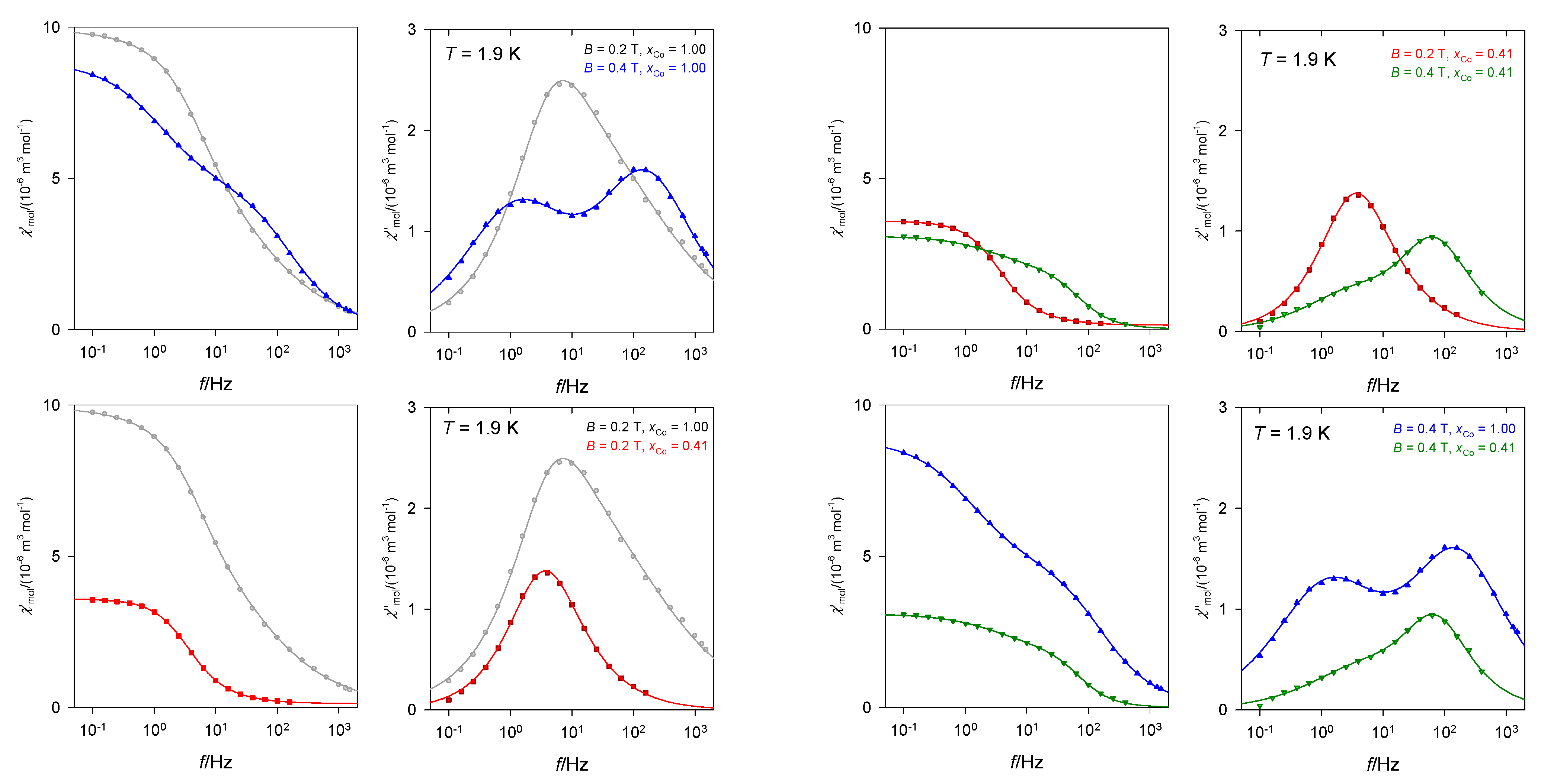
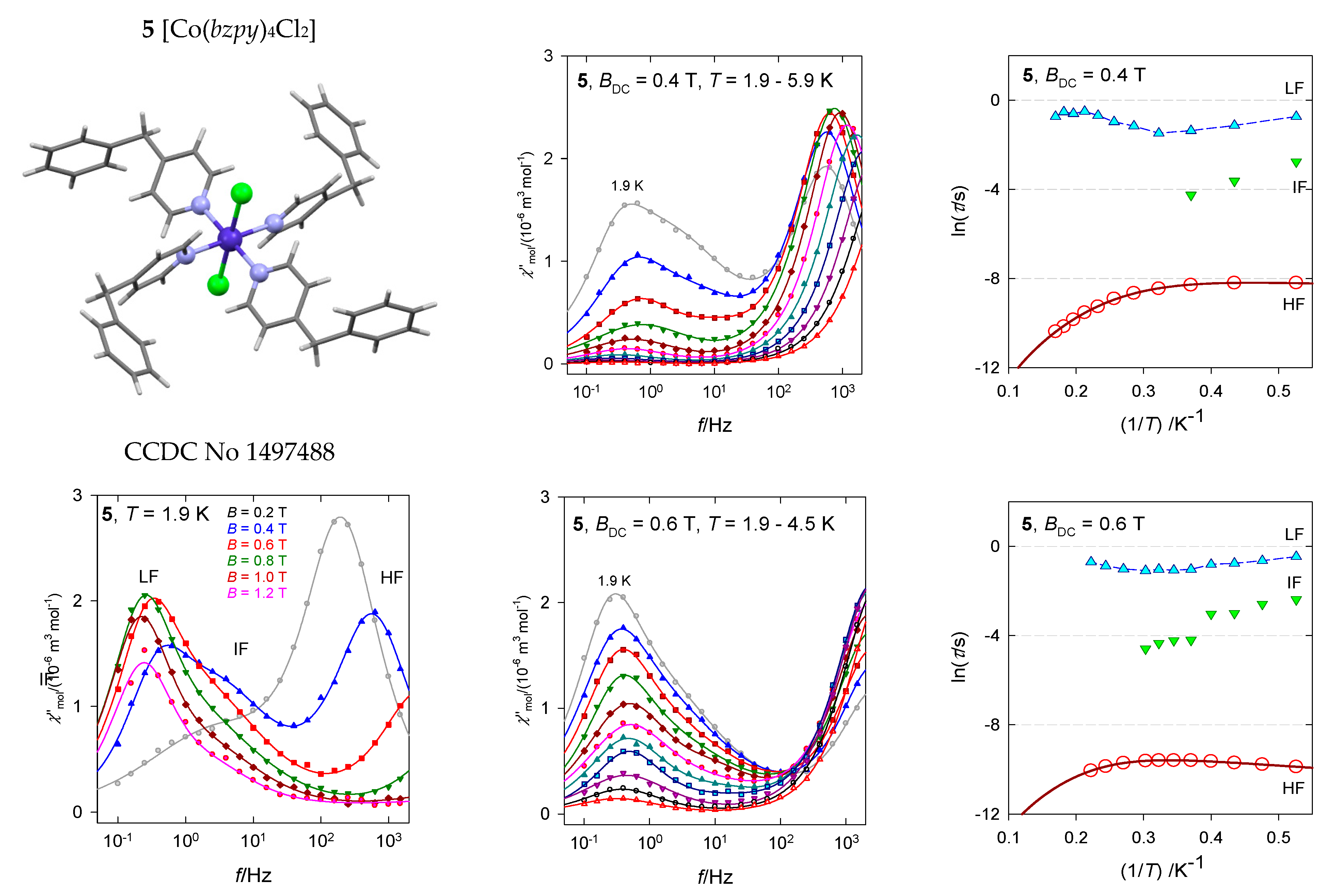
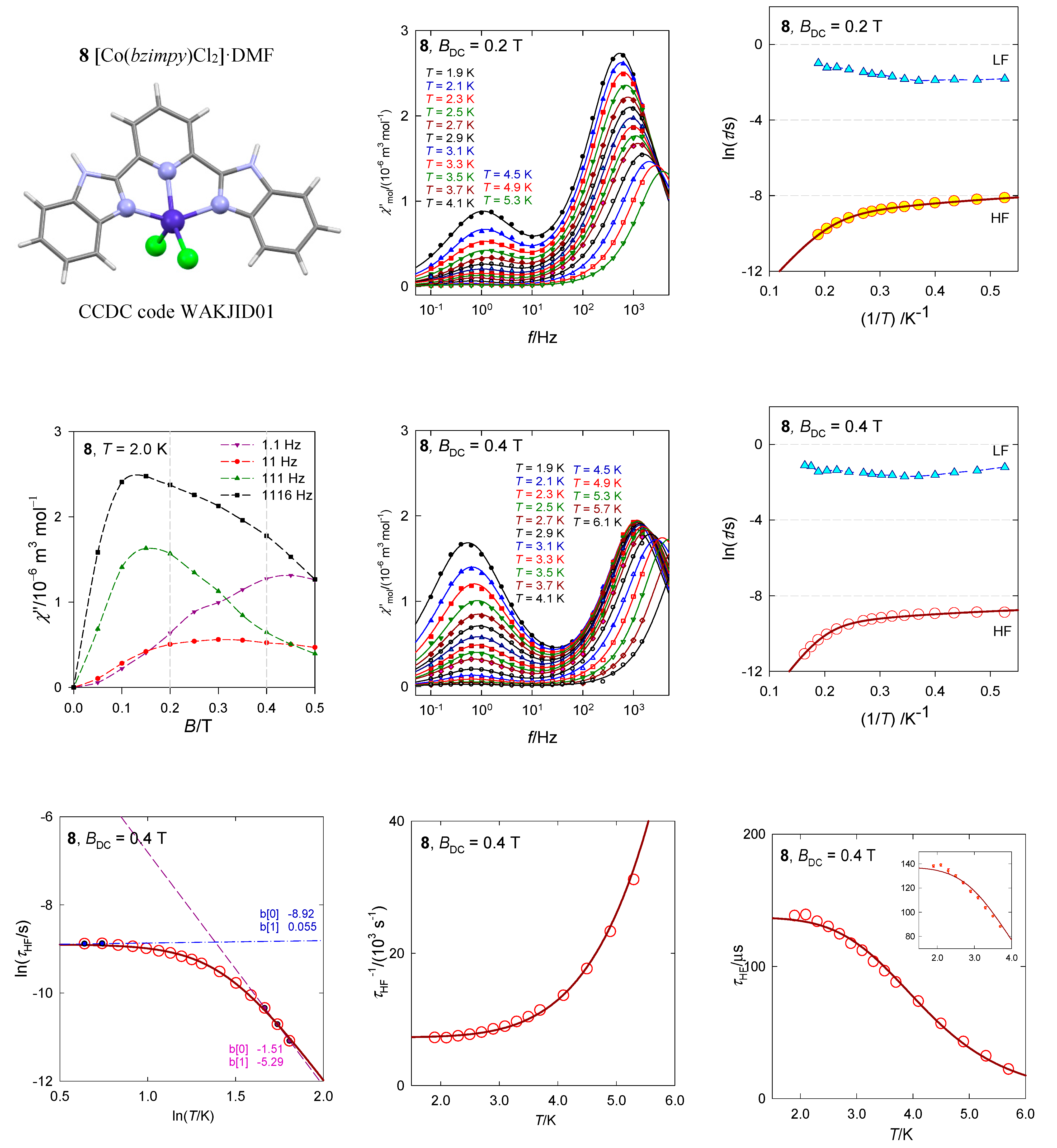
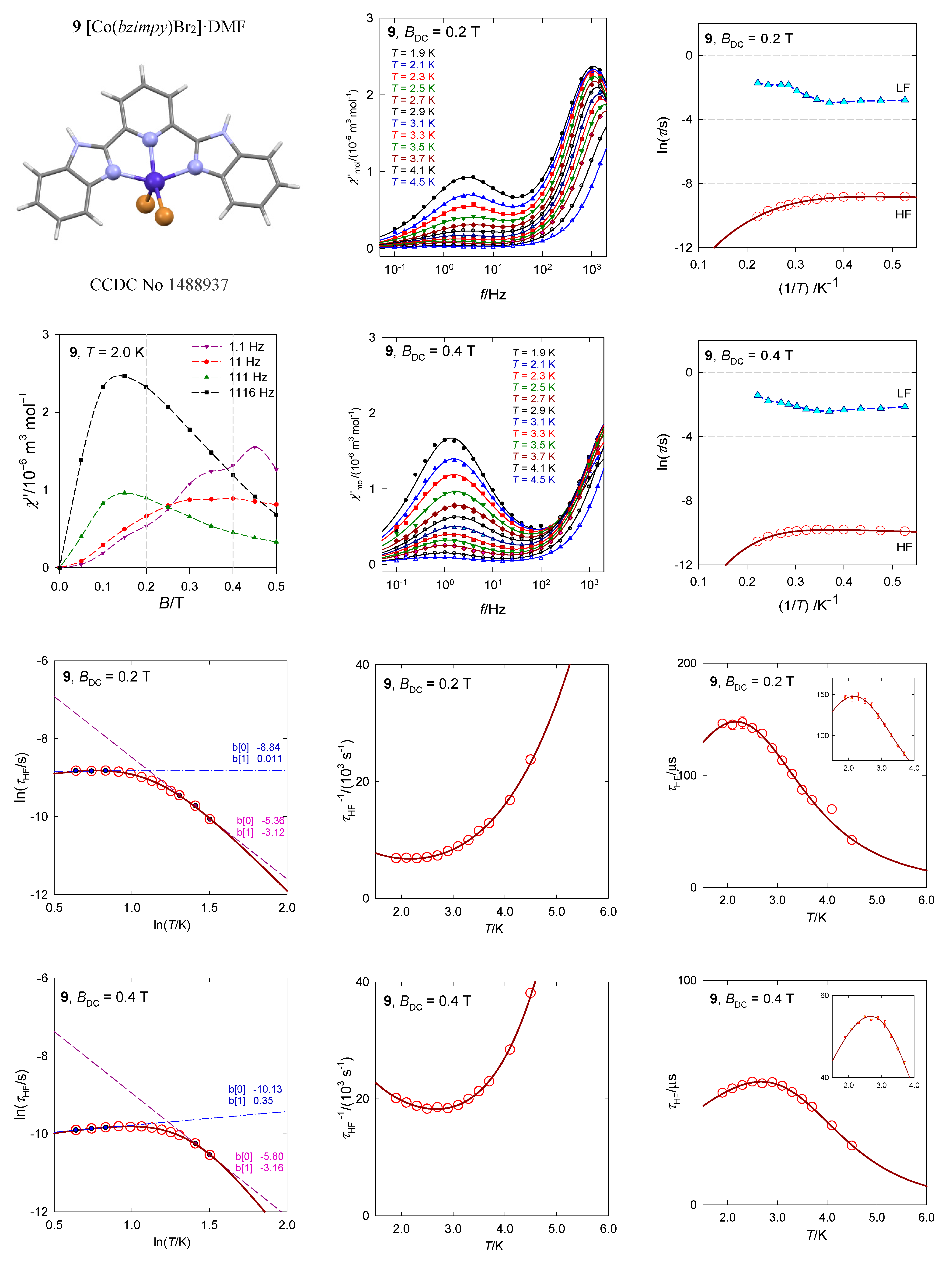
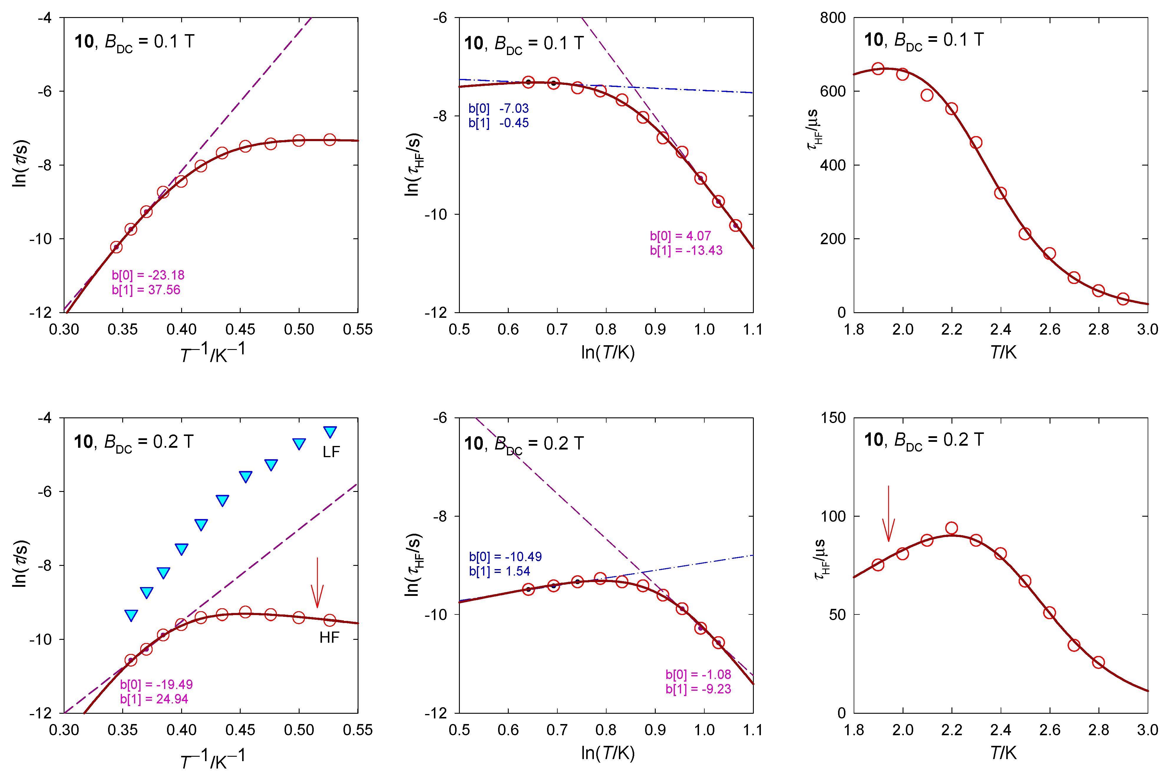
6.3. Cobalt(II) Complexes Showing RTB

The hexacoordinate complex [Co(pydca)(dmpy)]·0.5H₂O, 2, contains two structural units A and B, both resembling a compressed tetragonal bipyramid along the N–Co–N linkage with a significant angular distortion reducing the D_4h symmetry to D_2d (O–Co–O angles less than 180 deg). Ab initio CASSCF calculations using experimental geometries show that the lowest excited electronic terms lie at 797 and 2571 cm⁻¹ above the ground term for A as well as 389 and 1763 cm⁻¹ for B. These are daughter terms of the ⁴T_1g octahedral mother term on symmetry lowering to the ground ⁴E_g, that further splits into 1⁴A₁ and 2⁴A₁, whereas ⁴A_1g converts to 3⁴A₁. For the low energy gap, the subsequent evaluation of the spin-Hamiltonian parameters could fail in predicting the sign and value of the D-parameter and g_z component. Indeed, this is the case (see Table 2). The involvement of the spin-orbit interaction gave the energies of the lowest six Kramers doublets lying at δ = 0, 138, 971, 1176, 2753, and 2853 cm⁻¹ for A as well as δ = 0, 248, 731, 997, 2089, and 2212 cm⁻¹ for B. The D-value extracted from the DC magnetic data (magnetic susceptibility and magnetization) taking into account only the 1⁴A₁ ground electronic term is D/hc = 55 cm⁻¹ [26].

The first scan of the AC susceptibility (Figure 9a) shows that a maximum of the out-of-phase component appears for different frequencies at different fields. A more detailed mapping presented in Figure 9b confirms that three relaxation channels are in play. The external magnetic field supports the low-frequency channel at the expense of the high-frequency one that becomes suppressed. Notice, at T = 1.9 K and B_DC = 0.4 T the low-frequency relaxation time exceeds 1 s: τ(LF) = 1.3 s.

Figure 10 contains the AC susceptibility data of 22 ${\chi }^{\prime }(f)$ and 22 ${\chi }^{″}(f)$ data points for each temperature and the calculated convolution curve based upon 10 free parameters with acceptable standard deviations (

Table 5. Fitted parameters of the three-set Debye model for 2 at B_DC = 0.4 T including the discrepancy factors and standard deviations.

T/K	R(χ′)/%	R(χ″)/%	τLF/s	τIF/10−3 s	τHF/10−6 s	xLF	xHF
1.9	0.28	0.73	1.34(5)	107(11)	456(8)	0.28	0.14
2.1	0.32	1.1	1.08(2)	89(10)	474(8)	0.23	0.16
2.3	0.55	1.2	0.79(2)	74(21)	502(12)	0.21	0.19
2.5	0.57	1.5	0.67(3)	56(17)	533(14)	0.22	0.21
2.7	0.63	1.1	0.65(3)	56(23)	556(13)	0.14	0.25
2.9	0.31	1.3	0.55(2)	44(11)	579(8)	0.14	0.31
3.3	0.42	0.85	0.37(1)	30(11)	631(10)	0.20	0.46
3.7	0.21	0.92	0.31(1)	24(8)	615(5)	0.17	0.59
4.1	0.23	0.86	0.30(1)	18(10)	544(4)	0.14	0.69
4.5	0.19	0.93	0.31(1)	11(6)	500(3)	0.11	0.76
5.3	0.22	0.84	0.35(2)	7.4	267(1)	0.06	0.88
6.1	0.29	0.86	0.40(5)	3.0	144(1)	0.04	0.93
7.0	0.24	0.66	-	-	69(1)		1
8.0	0.14	1.7			32(1)		1
9.0	0.18	2.4			16(1)		1
10.0	0.31	5.3			8.4(7)		1

Mole fractions of the relaxing species: $x_{\mathrm{LF}}=({\chi }_{T,\mathrm{LF}}-{\chi }_S)/({\chi }_T-{\chi }_S)$, $x_{\mathrm{IF}}=({\chi }_{T,\mathrm{IF}}-{\chi }_{T,\mathrm{LF}})/({\chi }_T-{\chi }_S)$, $x_{\mathrm{HF}}=({\chi }_{T,\mathrm{HF}}-{\chi }_{T,\mathrm{IF}})/({\chi }_T-{\chi }_S)$, ${\chi }_{T,\mathrm{HF}}={\chi }_T$, and x_IF = 1 − x_LF − x_HF. R—discrepancy factors of fit for the in-phase and out-of-phase susceptibility. A digit in parentheses is the standard deviation. Bold—data showing RTB.

). There is an indication of the isosbestic point at f~40 Hz.

The fitted relaxation time τ_HF for the high-frequency channel on cooling from T = 10 K shows an increase in accordance with existing theories. However, it turns down below 4 K, which reflects an accelerated relaxation. This reciprocating thermal behavior cannot be reproduced by traditional relaxation mechanisms (Orbach, Raman, direct, quantum tunneling). A three-point linear fit in the Arrhenius-like diagram (Figure 10b) would predict the barrier to spin reversal U_eff = 2|D|~53 cm⁻¹. However, D > 0 detected by magnetometry does not support the Orbach relaxation mechanism.

The high-temperature data can be well fitted by assuming the Raman-like process as evidenced from the linear fit in Figure 10c. The temperature exponent in τ_Raman⁻¹ = CTⁿ is n = 5.9. The low-temperature tail of the relaxation time can be fitted well by assuming the second (LT) solution for the phonon bottleneck effect, τ_pb⁻¹ = FT^−k with k = 0.64 (not far from the theoretical value of 1). A fitting procedure based upon the combined formula ${\tau }^{-1}=C{T}^n+F{T}^{-k}$ gave a slightly modified value k = 0.78. The reconstructed function for the relaxation time passes through the “experimental” data almost perfectly within the standard deviations shown in Figure 10d.

Doping experiments of 2 into a diamagnetic matrix (Co:Zn = 1:3) disclosed that the former three relaxation channels collapse into a single one manifesting itself only in a single peak at χ″ vs. f and the RTB effect is lost (Figure 11). Therefore, the LF and eventually also IF channels are of the intermolecular nature and the RBT effect is somehow associated with the multichannel relaxation. An effect of the dilution to the diamagnetic matrix and the field dependence of the relaxation time supports the presence of a kind of direct process, including the PB [56].

Two hexacoordinate complexes with the same pincer-type structure, [Cu(pydca)(dmpy)] 0.5H₂O and [Ni(pydca)(dmpy)]·H₂O, also show RTB [53,54] (Table 3).

A complex [Co(dmpy)₂](dnbz)₂] containing 2,6-pyridinedimethanol in the coordination sphere and dinitrobenzoato anions also shows the slow magnetic relaxation, however, without RTB in the studied region of temperatures and magnetic fields [27]. The lnτ_HF vs. lnT dependence gave the temperature exponent l = 2.3 suggesting the phonon bottleneck relaxation process. There is a strong change in the slow magnetic relaxation upon doping to the diamagnetic Zn(II) matrix (Figure 12).

The hexacoordinate complex [Co(bzpy)₄Cl₂], 5, contains two structural units with the geometry of the tetragonally distorted octahedron (tetragonal bipyramid) [34]. Despite the fact that the axial Co-Cl distances are longer than four equatorial Co-N ones, the complex magnetically behaves as a compressed tetragonal bipyramid for which the spin-Hamiltonian formalism is justified. The ab initio calculations gave D/hc = 87 and 124 cm⁻¹, respectively, matching with the susceptibility and magnetization data D/hc = 106 cm⁻¹. It is unlikely that the observed slow magnetic relaxation would proceed at low temperature according to the Orbach mechanism since the energy gap of the ground and excited multiplets, Δ = 2D, is too high and moreover, D is unambiguously positive with no orthorhombic component E.

The available AC susceptibility data were successfully fitted by employing the three- or two-set Debye model and the extracted relaxation times are plotted in Figure 13 in several ways. The high-frequency relaxation channel can be analyzed using the combined formula ${\tau }^{-1}=G{T}^l+F{T}^{-k}$, where the parameter G is field dependent (unlike the true Raman process that is field independent). The results are listed in Table 3. The increased magnetic field: (i) Favors the low-frequency relaxation channel; (ii) separates the peaks at the LF and HF branches; and (iii) alters the relaxation parameters. The linear fits lnτ vs. lnT gave l = 3.7 and 2.1 for B_DC = 0.4 and 0.6 T, respectively, whereas the non-linear fitting procedure results in l = 4.2 and 3.7. These exponents are too low for the pure Raman process, however, they are too high for the net phonon bottleneck process. The evidence of RBT (probably a second solution of the phonon bottleneck effect) is magnified by the magnetic field: The parameter k increases in the monitored field range.

The hexacoordinate complex [Co(bzpy)₄(NCS)₂], 6, displays characteristics analogous to 5 [29]. Ab initio calculations predict D/hc = 88.6 and 90.8 cm⁻¹ for the two structural units matching the magnetometric determination D/hc = 90.5 cm⁻¹. These data again discriminate the presence of the Orbach relaxation process. The AC susceptibility confirms two relaxation channels (Figure 14): at B_DC = 0.2 T the LF channel is seen only as a shoulder at χ″ vs. f function, whereas at B_DC = 0.4 T it refers to a well-developed second, LF peak. The linearized graphs lnτ vs. lnT gave the exponents l = 4.1 and k~0, whereas the non-linear data fitting resulted in l = 4.3 and k = 0.4. These data are close to those obtained for [Co(bzpy)₄Cl₂] for the same external field B_DC = 0.4 T (Table 3).

The dinuclear complex [Co^IIICo^II(LH₂)₂(CH₃COO)(H₂O)](H₂O)₃, 7, contains the magnetically silent center Co(III) and the magnetically active center Co(II) possessing the {CoO₆} donor set (Figure 15) [35]. There are no symmetry elements within the chromophore so that the ground state is orbitally non-degenerate. However, it results from the splitting of the mother octahedral term ⁴T_2g to the {⁴E, ⁴A} daughter terms, and a further symmetry descent generates the three lowest orbital singlets. Ab initio calculations predict the three lowest energy terms lying at 0, 353, and 1250 cm⁻¹ by the CASSCF method and at 0, 463, and 1532 cm⁻¹ by further application of the NEVPT2 diagonal correction. This means that the ground electronic term is quasi degenerate and the application of the spin-Hamiltonian formalism needs to be assessed with care. After inclusion of the spin-orbit interaction, ORCA calculations gave six Kramers doublets lying at the energies 0, 219, 752, 1020, 1867, and 1942 cm⁻¹. The lowest energy gap δ₁ = 219 cm⁻¹ has no relationship to the axial zero-field splitting parameter D in the case of the quasi degenerate ground term. However, when the evaluation of the spin-Hamiltonian parameters is activated, incorrect predictions are obtained: D/hc = −99.6 cm⁻¹, E/D = 0.26, and g{1.82, 2.32, 3.08}.

The magnetic susceptibility data in the present case was fitted successfully by utilizing the Griffith-Figgis model with parameters (Aκλ)/hc = −176 cm⁻¹, g_L = −(Aκ) = −1.49, Δ_ax/hc = −711 cm⁻¹, Δ_rh/hc = 44 cm⁻¹. The magnetic anisotropy is of the easy-axis type as proven by the 3D visualization of the magnetization (the magnetic field was pointed to the set of grid points distributed uniformly over a sphere).

The AC susceptibility measurements show a two-channel slow magnetic relaxation: The low-frequency relaxation channel is strongly supported by the external magnetic field. Moreover, the RTB is evidenced at B_DC = 0.4 T and the relaxation time for the HF channel can be fitted with the temperature exponents l = 4.1 and k = 0.75.

The pentacoordinate complex [Co(bzimpy)Cl₂], 8, resembles the geometry of the square pyramid (the SHAPE agreement factor AF(SPY-5) = 1.7) rather than trigonal bipyramid (AF(TBPY-5) = 5.0), Figure 16 [40]. For the square pyramid of the C_4v symmetry the ground electronic term is orbitally degenerate ⁴E. Even at the lowered symmetry the ground and the first excited electronic terms could be quasi-degenerate (separated by~10² cm⁻¹) so that the spin Hamiltonian formalism is problematic to apply. An activation of the ab initio evaluation of the D-parameter could lead to false predictions, both in its value and sign. Indeed, the inappropriate calculation yields erroneous results D/hc = −87 cm⁻¹ and g_z = 1.86 that originate in the divergence of the perturbation theory (splitting of terms is only Δ/hc = 220 cm⁻¹). The multiplets (Kramers doublets) arising from the ground electronic term lie at 0, 186, 559, and 803 cm⁻¹, but the first gap δ/hc = 186 cm⁻¹ has nothing to do with the axial zero-field splitting parameter D.

The complex [Co(bzimpy)Br₂]·DMF, 9, most closely resembles a square pyramid, with the SHAPE agreement factor AF(SPY-5) = 2.1 (for trigonal bipyramid AF(TBPY-5) = 5.4), Figure 17 [40]. The ab initio calculations predict the first excited crystal field term at Δ/hc = 380 cm⁻¹ and the four lowest multiplets (Kramers doublets) positioned at δ = 0, 138, 632, and 819 cm⁻¹. The calculated value D/hc = 64 cm⁻¹ is not too far from the analysis of DC magnetic data, D/hc = 47 cm⁻¹. The calculated E/D = 0.24 points to an importance of the orthorhombic zfs-parameter E, but g_z = 1.93 is still underestimated. The AC susceptibility data show two relaxation channels with visible RTB. The temperature exponents are n = 4.0 (5.1) and k = 0.75 (0.56) for B_DC = 0.2 and 0.4 T, respectively.

The mononuclear complex [Co^II(PPh₃)₂Br₂], 10, is a tetracoordinate system with rather large negative axial zero-field splitting parameter D/hc = −13 cm⁻¹ [47]. Since a non-zero out-of-phase susceptibility even at the zero DC field exists, this is a true single-molecule magnet (Figure 18) showing a single relaxation mode. With increasing external field, a low-frequency relaxation channel is opened that is well developed at B_DC = 0.2 T.

The relaxation time has been plotted in several ways as displayed in Figure 19. Three points from the high-temperature edge of lnτ vs. T⁻¹ dependence serve for a linear fit yielding the barrier to spin reversal U_eff/k_B = 38 and 25 K at B_DC = 0.1 and 0.2 T, respectively. When the Raman relaxation process is probed as an alternative, τ⁻¹ = CTⁿ, then the linear plot lnτ vs. lnT yields exponents n = 13 and 9 that are far above the border of acceptance for the Raman relaxation process. The RTB behavior is well seen in Figure 19: The relaxation time τ vs. T on cooling increases with expectations but then decreases at B_DC = 0.2 T.

The AC susceptibility shows two relaxation channels and the DC magnetic field supports the low-frequency branch. Again, the LF–HF peak separation is observed with the increasing field. At B_DC = 0.2 T, the RTB is not evidenced as opposite to B_DC = 0.4 T where its on-set is seen. The higher-temperature data can be fitted with the Raman-like term τ_Raman⁻¹ = CTⁿ with n = 5.3.

The tetracoordinate complex [Co(biq)Cl₂], 11, possesses the ground electronic term ⁴A₁ [33] which, according to ab initio calculations, is separated from the first excited term by Δ₁ = 1928 cm⁻¹. The calculated value D/hc = 16.1 cm⁻¹ is comparable with the magnetometric analysis yielding D/hc = 10.5 cm⁻¹. The field dependence of the AC susceptibility shows that the out-of-phase component exhibits maxima that depend upon the frequency of the oscillating field (Figure 20). Two external fields, B_DC = 0.2 and 0.3 T were selected for subsequent experiments. A detailed scan of the AC susceptibility for 22 frequencies ranging between f = 0.1 and 1500 Hz is presented in Figure 20. For B_DC = 0.2 T the dominant HF peak is accompanied by a minor LF peak and/or shoulder. However, with B_DC = 0.3 T the LF peak adopts its significance and competes the HF peak. On heating the extinction of the LF peak is faster than that of the HF peak.

The in-phase and out-of-phase susceptibility components have been fitted by employing the two-set Debye model with seven parameters. Two primitive functions merge to a convoluted envelope that is drawn in Figure 20 as a full line, which passes through the experimental points almost perfectly. The slow magnetic relaxation shows features of the RTB and the relaxation time at B_DC = 0.3 T can be fitted with the temperature exponents n = 12.0 and k = 1.0 (Figure 20). A possible Orbach relaxation mechanism is discriminated by positive D. RTB is not identified for B_DC = 0.2 T.

7. Conclusions

The slow magnetic relaxation in mononuclear Co(II) complexes often proceed through two relaxation channels: Low- and high-frequency mode. The external magnetic field supports the low-frequency channel, i.e., the maximum at the out-of-phase susceptibility is moved to lower frequencies (a longer relaxation time), whereas the opposite effect exhibits the high-frequency channel. Some of these complexes show the reciprocating thermal behavior in which a prolongation of the relaxation time on cooling passes through a maximum and then exhibits an acceleration at very low temperatures. Such a behavior cannot be modelled by the traditional relaxation mechanisms covering the Orbach, Raman, direct, and quantum tunneling processes since all of them exhibit positive temperature exponentsτ⁻¹~Tⁿ, n > 0. RTB, on the contrary, requires τ⁻¹~T^−k, k > 0 and the only theoretical support so far is given by the second solution of the phonon bottleneck effect. However, one can speculate about an alternate hypothesis: The presence of the LF relaxing species causes the concentration of the HF relaxing units to decrease and such a dilution, eventually, can facilitate the relaxation rate.

References

1. Gatteschi, D.; Sessoli, R.; Villain, J. Molecular Nanomagnets; Oxford University Press: Oxford, UK, 2006; ISBN 13 9780198567530. [Google Scholar]
2. Winpenny, R. (Ed.) Single-Molecule Magnets and Related Phenomena; Springer: Berlin/Heidelberg, Germany, 2006; Volume 122, ISBN 978-3-540-33239-8. [Google Scholar]
3. Benelli, C.; Gatteschi, D. Introduction to Molecular Magnetism: From Transition Metals to Lanthanides; Wiley: Weinheim, Germany, 2015; ISBN 978-3-527-33540-4. [Google Scholar]
4. Atanasov, M.; Zadrozny, J.M.; Long, J.R.; Neese, F. A theoretical analysis of chemical bonding, vibronic coupling, and magnetic anisotropy in linear iron(II) complexes with single-molecule magnet behavior. Chem. Sci. 2013, 4, 139–156. [Google Scholar] [CrossRef]
5. Layfield, R.A. Organometallic Single-Molecule Magnets. Organometallics 2014, 33, 1084–1099. [Google Scholar] [CrossRef]
6. Wernsdorfer, W.; Sessoli, R. Quantum Phase Interference and Parity Effects in Magnetic Molecular Clusters. Science 1999, 284, 133–135. [Google Scholar] [CrossRef] [Green Version]
7. Rinehart, J.D.; Long, J.R. Exploiting Single-Ion Anisotropy in the Design of f-element Single-Molecule Magnets. Chem. Sci. 2011, 2, 2078–2085. [Google Scholar] [CrossRef]
8. Gatteschi, D.; Barra, A.L.; Caneschi, A.; Cornia, A.; Sessoli, R.; Sorace, L. EPR of Molecular Nanomagnets. Coord. Chem. Rev. 2006, 250, 1514–1529. [Google Scholar] [CrossRef]
9. Meng, Y.-S.; Jiang, S.-D.; Wang, B.-W.; Gao, S. Understanding the Magnetic Anisotropy toward Single-Ion Magnets. Acc. Chem. Res. 2016, 49, 2381–2389. [Google Scholar] [CrossRef] [PubMed]
10. Liddle, S.T.; van Slageren, J. Improving f-element single molecule magnets. J. Chem. Soc. Rev. 2015, 44, 6655–6669. [Google Scholar] [CrossRef] [Green Version]
11. Woodruff, D.N.; Winpenny, R.E.P.; Layfield, R.A. Lanthanide Single-Molecule Magnets. Chem. Rev. 2013, 113, 5110–5148. [Google Scholar] [CrossRef]
12. Coulon, C.; Miyasaka, H.; Clérac, R. Single-Chain Magnets: Theoretical Approach and Experimental Systems. Struct. Bonding 2006, 122, 163–206. [Google Scholar] [CrossRef]
13. Craig, G.A.; Murrie, M. 3d single ion magnets. Chem. Soc. Rev. 2015, 44, 2135–2147. [Google Scholar] [CrossRef] [Green Version]
14. Gómez-Coca, S.; Aravena, D.; Morales, R.; Ruiz, E. Large magnetic anisotropy in mononuclear metal complexes. Coord. Chem. Rev. 2015, 289–290, 379–392. [Google Scholar] [CrossRef] [Green Version]
15. Frost, J.M.; Harriman, K.L.M.; Murugesu, M. The rise of 3-d single-ion magnets in molecular magnetism: Towards materials from molecules. Chem. Sci. 2016, 7, 2470–2491. [Google Scholar] [CrossRef] [Green Version]
16. Boča, R.; Rajnák, C. Unexpected behavior of single ion magnets. Coord. Chem. Rev. 2021, 430, 213657. [Google Scholar] [CrossRef]
17. Rajnák, C.; Boča, R. Reciprocating thermal behavior in the family of single ion magnets. Coord. Chem. Rev. 2021, 436, 213808. [Google Scholar] [CrossRef]
18. Abragam, A.; Bleaney, B. Electron Paramagnetic Resonance of Transition Ions; Clarendon Press: Oxford, UK, 1970. [Google Scholar]
19. Standley, K.J.; Vaughan, R.A. Electron Spin Relaxation Phenomena in Solids; Plenum Press: New York, NY, USA, 1969. [Google Scholar] [CrossRef]
20. Van Vleck, J.H. Paramagnetic Relaxation Times for Titanium and Chrome Alum. Phys. Rev. 1940, 57, 426–447. [Google Scholar] [CrossRef]
21. Zadrozny, J.M.; Atanasov, M.; Bryan, A.M.; Lin, C.-Y.; Rekken, B.D.; Power, P.P.; Neese, F.; Long, J.R. Slow magnetization dynamics in a series of two-coordinate iron(II) complexes. Chem. Sci. 2013, 4, 125–138. [Google Scholar] [CrossRef]
22. Sato, H.; Kathirvelu, V.; Fielding, A.; Blinco, J.P.; Micallef, A.S.; Bottle, S.E.; Eaton, S.S.; Eaton, G.R. Impact of molecular size on electron spin relaxation rates of nitroxyl radicals in glassy solvents between 100 and 300K. Mol. Phys. 2007, 105, 2137–2151. [Google Scholar] [CrossRef] [Green Version]
23. Abtab, S.M.T.; Majee, M.C.; Maity, M.; Titiš, J.; Boča, R.; Chaudhury, M. Tetranuclear Hetero-Metal [CoII2LnIII2] (Ln = Gd, Tb, Dy, Ho, La) Complexes Involving Carboxylato Bridge in a Rare µ4-η2:η2 Mode: Synthesis, Crystal Structures and Magnetic Properties. Inorg. Chem. 2014, 53, 1295–1306. [Google Scholar] [CrossRef] [PubMed]
24. Scott, P.L.; Jeffries, C.D. Spin-Lattice Relaxation in Some Rare-Earth Salts at Helium Temperatures; Observation of the Phonon Bottleneck. Phys. Rev. 1962, 127, 32–51. [Google Scholar] [CrossRef]
25. Tesi, L.; Lunghi, A.; Atzori, M.; Lucaccini, E.; Sorace, L.; Totti, F.; Sessoli, R. Giant spin-phonon bottleneck effects in evaporable vanadylbased molecules with long spin coherence. Dalton Trans. 2016, 45, 16635–16643. [Google Scholar] [CrossRef]
26. Boča, R.; Rajnák, C.; Moncoľ, J.; Titiš, J.; Valigura, D. Breaking the Magic Border of One Second for Slow Magnetic Relaxation of Cobalt-Based Single Ion Magnets. Inorg. Chem. 2018, 57, 14314–14321. [Google Scholar] [CrossRef]
27. Valigura, D.; Rajnák, C.; Moncoľ, J.; Titiš, J.; Boča, R. A mononuclear Co(II) complex formed of pyridinedimethanol with manifold slow relaxation channels. Dalton Trans. 2017, 46, 10950–10956. [Google Scholar] [CrossRef]
28. Casimir, H.B.G.; DuPre, F.K. Note on the thermodynamic interpretation of paramagnetic relaxation phenomena. Physica 1935, 5, 507–511. [Google Scholar] [CrossRef]
29. Cole, K.S.; Cole, R.H. Dispersion and absorption in dielectrics I. Alternating current characteristics. J. Chem. Phys. 1941, 9, 341–352. [Google Scholar] [CrossRef] [Green Version]
30. Boča, R. A Handbook of Magnetochemical Formulae; Elsevier: Amsterdam, The Netherlands, 2012. [Google Scholar] [CrossRef]
31. Boča, R. Struct. Bonding; Springer: Berlin/Heidelberg, Germany, 2006; Volume 117. [Google Scholar] [CrossRef]
32. Neese, F. The ORCA program system. WIREs Comput. Mol. Sci. 2012, 2, 73–78. [Google Scholar] [CrossRef]
33. Smolko, L.; Černák, J.; Dušek, M.; Miklovič, J.; Titiš, J.; Boča, R. Three tetracoordinate Co(II) complexes [Co(biq)X2] (X = Cl, Br, I) with easy-plane magnetic anisotropy as field-induced single-molecule magnets. Dalton Trans. 2015, 44, 17565–17571. [Google Scholar] [CrossRef] [PubMed]
34. Rajnák, C.; Titiš, J.; Moncoľ, J.; Renz, F.; Boča, R. Field-Supported Slow Magnetic Relaxation in Hexacoordinate CoII Complexes with Easy Plane Anisotropy. Eur. J. Inorg. Chem. 2017, 2017, 1520–1525. [Google Scholar] [CrossRef]
35. Buvaylo, E.A.; Kokozay, V.N.; Vassilyeva, O.Y.; Skelton, B.W.; Ozarowski, A.; Titiš, J.; Vranovičová, B.; Boča, R. Field-Assisted Slow Magnetic Relaxation in a Six-Coordinate Co(II)–Co(III) Complex with Large Negative Anisotropy. Inorg. Chem. 2017, 56, 6999–7009. [Google Scholar] [CrossRef]
36. Rajnák, C.; Varga, F.; Titiš, J.; Moncoľ, J.; Boča, R. Octahedral-tetrahedral systems [Co(dppmO,O)3]2+[CoX4]2− showing slow magnetic relaxation with two relaxation modes. Inorg. Chem. 2018, 57, 4352–4358. [Google Scholar] [CrossRef] [PubMed]
37. Varga, F.; Rajnák, C.; Titiš, J.; Moncol’, J.; Boča, R. Slow magnetic relaxation in a Co(II) octahedral-tetrahedral system formed of a [CoL3]2+ core with L = bis(diphenylphosphanoxido) methane and tetrahedral [CoBr4]2− counter anions. Dalton Trans. 2017, 46, 4148–4151. [Google Scholar] [CrossRef]
38. Packová, A.; Miklovič, J.; Boča, R. Manifold Relaxation Processes in a Mononuclear Co(II) Single-Molecule Magnet. Polyhedron 2015, 102, 88–93. [Google Scholar] [CrossRef]
39. Ruamps, R.; Batchelor, L.J.; Guillot, R.; Zakhia, G.; Barra, A.L.; Wernsdorfer, W.; Guihery, N.; Mallah, T. Ising-type magnetic anisotropy and single molecule magnet behaviour in mononuclear trigonal bipyramidal Co(ii) complexes. Chem. Sci. 2014, 5, 3418–3424. [Google Scholar] [CrossRef]
40. Rajnák, C.; Varga, F.; Titiš, J.; Moncoľ, J.; Boča, R. Field-Supported Single-Molecule Magnets of Type [Co(bzimpy)X2]. Eur. J. Inorg. Chem. 2017, 2017, 1915–1922. [Google Scholar] [CrossRef]
41. Rajnák, C.; Titiš, J.; Miklovič, J.; Kostakis, G.E.; Fuhr, O.; Ruben, M.; Boča, R. Five mononuclear pentacoordinate Co(II) complexes as field-induced single molecule magnets. Polyhedron 2017, 126, 174–183. [Google Scholar] [CrossRef]
42. Mandal, S.; Mondal, S.; Rajnák, C.; Titiš, J.; Boča, R.; Mohanta, S. Syntheses, crystal structures and magnetic properties of two mixed-valence Co(III)Co(II) compounds derived from Schiff base ligands: Field supported single-ion-magnet behaviour with easy plane anisotropy. Dalton Trans. 2017, 46, 13135–13144. [Google Scholar] [CrossRef]
43. Rajnák, C.; Packová, A.; Titiš, J.; Miklovič, J.; Moncoľ, J.; Boča, R. A tetracoordinate Co(II) single molecule magnet based on triphenylphosphine and isothiocyanato group. Polyhedron 2016, 110, 85–92. [Google Scholar] [CrossRef]
44. Yang, F.; Zhou, Q.; Zhang, Y.; Zeng, G.; Li, G.; Shi, Z.; Wang, B.; Feng, S. Inspiration from old molecules: Field-induced slow magnetic relaxation in three air-stable tetrahedral cobalt(ii) compounds. Chem. Commun. 2013, 49, 5289–5291. [Google Scholar] [CrossRef]
45. Titiš, J.; Miklovič, J.; Boča, R. Magnetostructural study of tetracoordinate cobalt(II) complexes. Inorg. Chem. Commun. 2013, 35, 72–75. [Google Scholar] [CrossRef]
46. Krzystek, J.; Zvyagin, S.A.; Ozarowski, A.; Fiedler, A.T.; Brunold, T.C.; Telser, J. Definitive Spectroscopic Determination of Zero-Field Splitting in High-Spin Cobalt(II). J. Am. Chem. Soc. 2004, 126, 2148. [Google Scholar] [CrossRef]
47. Boča, R.; Miklovič, J.; Titiš, J. Simple Mononuclear Cobalt(II) Complex: A Single-Molecule Magnet Showing Two Slow Relaxation Processes. Inorg. Chem. 2014, 53, 2367–2369. [Google Scholar] [CrossRef] [PubMed]
48. Saber, M.R.; Dunbar, K.R. Ligands effects on the magnetic anisotropy of tetrahedral cobalt complexes. Chem. Commun. 2014, 50, 12266–12269. [Google Scholar] [CrossRef]
49. Smolko, L.; Černák, J.; Dušek, M.; Titiš, J.; Boča, R. Tetracoordinate Co(II) Complexes Containing Bathocuproine and Single Molecule Magnetism. New J. Chem. 2016, 40, 6593–6598. [Google Scholar] [CrossRef]
50. Huang, W.; Liu, T.; Wu, D.; Cheng, J.; Ouyang, Z.W.; Duan, C. Field-induced slow relaxation of magnetization in a tetrahedral Co(ii) complex with easy plane anisotropy. Dalton Trans. 2013, 42, 15326–15331. [Google Scholar] [CrossRef]
51. Smolko, L.; Černák, J.; Kuchár, J.; Rajnák, C.; Titiš, J.; Boča, R. Field-Induced Slow Magnetic Relaxation in Mononuclear Tetracoordinate Cobalt(II) Complexes Containing a Neocuproine Ligand. Eur. J. Inorg. Chem. 2017, 2017, 3080–3086. [Google Scholar] [CrossRef]
52. Rajnák, C.; Titiš, J.; Moncol, J.; Mičová, R.; Boča, R. Field induced slow magnetic relaxation in a mononuclear Mn(II) complex. Inorg. Chem. 2019, 58, 991–994. [Google Scholar] [CrossRef] [PubMed]
53. Boča, R.; Rajnák, C.; Titiš, J.; Valigura, D. Field Supported Slow Magnetic Relaxation in a Mononuclear Cu(II) Complex. Inorg. Chem. 2017, 56, 1478–1482. [Google Scholar] [CrossRef]
54. Titiš, J.; Rajnák, C.; Valigura, D.; Boča, R. Field influence on the slow magnetic relaxation of nickel-based single ion magnets. Dalton Trans. 2018, 47, 7879–7882. [Google Scholar] [CrossRef]
55. Atzori, M.; Tesi, L.; Morra, E.; Chiesa, M.; Sorace, L.; Sessol, R. Room-Temperature Quantum Coherence and Rabi Oscillations in Vanadyl Phthalocyanine: Toward Multifunctional Molecular Spin Qubits. J. Am. Chem. Soc. 2016, 138, 2154–2157. [Google Scholar] [CrossRef]
56. Rousset, E.; Piccardo, M.; Boulon, M.E.; Gable, R.W.; Soncini, A.; Sorace, L.; Boskovic, C. Slow Magnetic Relaxation in Lanthanoid Crown Ether Complexes: Interplay of Raman and Anomalous Phonon Bottleneck Processes. Chem. A Eur. J. 2018, 24, 14768–14785. [Google Scholar] [CrossRef] [Green Version]
57. Ray, R.; Avdoshenko, S.M. Insights in Magnetodynamics from a Simple Two-Level Model. ChemRxiv 2020. [Google Scholar] [CrossRef]
58. Balanda, M. AC Susceptibility Studies of Phase Transitions and Magnetic Relaxation: Conventional, Molecular and Low-Dimensional Magnets. Acta Phys. Pol. 2013, 124, 964–976. [Google Scholar] [CrossRef]
59. Freude, D.; Haase, J. Quadrupole Effects in Solid-State Nuclear Magnetic Resonance. In Special Applications; NMR Basic Principles and Progress Series; Pfeifer, H., Barker, P., Eds.; Springer: Berlin/Heidelberg, Germany, 1993; Volume 29. [Google Scholar] [CrossRef]
60. Chiorescu, I.; Wernsdorfer, W.; Müller, A.; Bögge, H.; Barbara, B. Butterfly Hysteresis Loop and Dissipative Spin Reversal in the S = 1/2, V15 Molecular Complex. Phys. Rev. Lett. 2000, 84, 3454–3457. [Google Scholar] [CrossRef] [Green Version]
61. Madsen, D.E.; Hansen, M.F.; Mørup, S. The correlation between superparamagnetic blocking temperatures and peak temperatures obtained from ac magnetization measurements. J. Phys. Condens. Matt. 2008, 20, 345209. [Google Scholar] [CrossRef]
Figure 1. Different contributions to the relaxation time in [DyIII2ZnII2] molecular complex: Orbach (high-temperature, blue, Ueff/kB = 53 K), Raman (intermediate-temperature, black, n~5), phonon bottleneck (low temperature, green, n~2), direct (low-temperature, red, n~1), quantum tunneling of magnetization (violet, n~0). Straight lines: y = b[0] + b[1]x. Data adapted from ref. [23]. 2014, American Chemical Society.
Magnetochemistry 07 00076 g001
Figure 2. Energy flow from the spin system through the phonon system to the thermal bath.
Magnetochemistry 07 00076 g002
Figure 3. Ways of AC susceptibility data taking/analysis. AC susceptibility components: (a) field dependence, (b) temperature dependence, (c,d) frequency dependence. Data adapted from ref. [27]. 2017, Royal Society of Chemistry.
Magnetochemistry 07 00076 g003
Figure 4. Frequency dependence of the AC susceptibility according to the two-set Debye model. (a) Envelope of AC susceptibility components. (b) Ideal Argand diagram (α1 = α2 = 0) with two overlapping semicircles.
Magnetochemistry 07 00076 g004
Figure 5. Test of the stability of the fitted relaxation time when 1 to 9 data points from the HF range are gradually omitted. Solid lines for individual fits are overlapped. Dashed lines: Primitive low-frequency (LF) and high-frequency (HF) components. Data adapted from ref. [33] for [Co(biq)Cl2], 12. 2015, Royal Society of Chemistry.
Magnetochemistry 07 00076 g005
Figure 6. Energy level diagrams for high-spin Co(II) complexes. Crystal field terms are labelled according to the Mulliken notation (A, B, E), the crystal field multiplets according to Bethe (Γi) as irreducible representations of the double group.
Magnetochemistry 07 00076 g006
Figure 7. Frequency dependence of the out-of-phase susceptibility at various temperatures and external fields for [Mn(bzpy)4Cl2]. (a) Left—full scale of data taking, right—zoomed high-frequency range truncated for clarity. Solid lines—fitted. (b) field dependence. Vertical mark envisages the maximum on χ″; notice its movement on heating to a slower relaxation and then back to the faster one. Data adapted from ref. [52]. 2019, American Chemical Society.
Magnetochemistry 07 00076 g007
Figure 8. Various dependences of the high-frequency relaxation time in [Mn(bzpy)4Cl2]. Full line—fitted over the whole temperature range with τ 1 = G T l + F T k . (a) Arrhenius-like plot, (b) log-log plot, (c) relaxation time vs temperature. The standard deviations for each data point are displayed in the inset of panel (c). Data adapted from ref. [52]. 2019, American Chemical Society.
Magnetochemistry 07 00076 g008
Figure 9. AC susceptibility and relaxation time for 2. Solid lines—fitted. (a) field dependence, (b) frequency depenence, (c) relaxation time vs. field.
Magnetochemistry 07 00076 g009
Figure 10. AC susceptibility and relaxation times for 2. Full lines—fitted. Hydrogen atoms are omitted hereafter. (a) Left—full scale of data taking, right—zoomed high-frequency range truncated for clarity. (b) Arrhenius-like plot, (c) log-log plot, (d) relaxation time vs. temperature (inset includes the standard deviations as error bars). Data adapted from ref. [26]. 2018, American Chemical Society.
Magnetochemistry 07 00076 g010
Figure 11. AC susceptibility for a doped sample C28H26Co0.52N4O13Zn1.48 (2b).
Magnetochemistry 07 00076 g011
Figure 12. AC susceptibility for [Co(dmpy)2](dnbz)2] (xCo = 1.00) and its doped analogue C28H24Co0.41N6O16Zn0.59 (xCo = 0.41). Data adapted from ref. [27]. 2017, Royal Society of Chemistry.
Magnetochemistry 07 00076 g012
Figure 13. AC susceptibility for 5. Full lines—fitted. Data adapted from ref. [34]. 2017, Wiley-VCH.
Magnetochemistry 07 00076 g013aMagnetochemistry 07 00076 g013b
Figure 14. AC susceptibility data for 6. Full lines—fitted. Data adapted from ref. [34]. 2017, Wiley-VCH.
Magnetochemistry 07 00076 g014aMagnetochemistry 07 00076 g014b
Figure 15. AC susceptibility data for 7. Full lines—fitted. Data adapted from ref. [35]. 2017, American Chemical Society.
Magnetochemistry 07 00076 g015aMagnetochemistry 07 00076 g015b
Figure 16. AC susceptibility data for 8. Full lines—fitted. Data adapted from ref. [40]. 2017, Wiley-VCH.
Magnetochemistry 07 00076 g016
Figure 17. AC susceptibility data for 9. Full lines—fitted. Data adapted from ref. [40]. 2017, Wiley-VCH.
Magnetochemistry 07 00076 g017
Figure 18. Frequency dependence of the out-of-phase susceptibility at various temperatures and external fields for [Co(PPh3)2Br2], 10. Solid lines—fitted; dashed—guide for eyes. Data adapted from ref. [47]. 2014, American Chemical Society.
Magnetochemistry 07 00076 g018
Figure 19. Various dependences of the high-frequency relaxation time in 10. Dashed/dot-dashed—linear fits. Full line—fitted over the whole temperature range using τ 1 = C T n + F T k . An arrow indicates the RTB behavior.
Magnetochemistry 07 00076 g019
Figure 20. AC susceptibility data for 11. Full lines—fitted. Data adapted from ref. [33]. 2015, Royal Society of Chemistry.
Magnetochemistry 07 00076 g020aMagnetochemistry 07 00076 g020b