Abstract
Wall-flow filters are applied in the exhaust treatment of internal combustion engines for the removal of particulate matter (PM). Over time, the pressure drop inside those filters increases due to the continuously introduced solid material, which forms PM deposition layers on the filter substrate. This leads to the necessity of regenerating the filter. During such a regeneration process, fragments of the PM layers can potentially rearrange inside single filter channels. This may lead to the formation of specific deposition patterns, which affect a filter’s pressure drop, its loading capacity and the separation efficiency. The dynamic formation process can still not consistently be attributed to specific influence factors, and appropriate calculation models that enable a quantification of respective factors do not exist. In the present work, the dynamic rearrangement process during the regeneration of a wall-flow filter channel is investigated. As a direct sequel to the investigation of a static deposition layer in a previous work, the present one additionally investigates the dynamic behaviour following the detachment of individual layer fragments as well as the formation of channel plugs. The goal of this work is the extension of the resolved particle methodology used in the previous work via a discrete method to treat particle–particle and particle–wall interactions in order to evaluate the influence of the deposition layer topology, PM properties and operating conditions on dynamic rearrangement events. It can be shown that a simple mean density methodology represents a reproducible way of determining a channel plug’s extent and its average density, which agrees well with values reported in literature. The sensitivities of relevant influence factors are revealed and their impact on the rearrangement process is quantified. This work contributes to the formulation of predictions on the formation of specific deposition patterns, which impact engine performance, fuel consumption and service life of wall-flow filters.
1. Introduction
Modern exhaust treatment systems of internal combustion engines rely on wall-flow filters as one of the key components for enabling compliance with present emission limits [1]. In such filters, a porous structure comprised of oppositely arranged inlet and outlet channels traps the contained particulate matter (PM) with efficiencies of up to 99% [2]. With increased filter loading, deposition layers are formed on the porous walls’ surfaces and the filter’s pressure drop increases, accompanied by a degradation of engine performance [3,4,5]. The introduced PM mostly consists of combustible soot and small amounts of inorganic non-combustible ash, which allows the filter’s regeneration by continuously or periodically oxidizing its reactive components. The regeneration affects the deposition layer composition over the long term, as it leads to an accumulation of ash, which eventually forms larger agglomerates. The resulting inhomogeneities can then lead to a break-up of the continuous layer into individual PM layer fragments, which potentially detach from the filter surface and relocate inside a channel [3]. This leads to the formation of specific deposition patterns, which affect a single channel’s pressure drop contribution, its loading capacity and the separation efficiency.
Various scientific works [4,6,7,8] contribute to the identification of probable causes and influence factors leading to the individual patterns, but a universal and consistent formulation without partially contradictory statements cannot be found. Calculation models that enable a consistent quantification of relevant influence factors on the individual parts of the regeneration process are missing completely. Those are, however, vital for respective predictions on the formation of specific deposition patterns, which impact engine performance, fuel consumption and service life of wall-flow filters.
In order to close this gap, the authors of the present manuscript approached different relevant aspects in three previous, consecutive works [9,10,11]: In an initial work [9], a holistic lattice Boltzmann method (LBM) approach was presented, which can be employed both for the simulation of the movement of surface resolved particles and the flow through porous media. With it, the gas flow and the movement of PM layer fragments was simulated with the open source software OpenLB [12,13], while super-linear grid convergence and good agreement with a reference solution [14] could be shown. A literature review addressing relevant findings on the deposition pattern formation, general numeric approaches to wall-flow filter modelling and LBM-related research regarding flow through porous media, as well as surface resolved particle simulations, can be found in this work. The approach was then used in a following work [10] for the investigation of the detachment, acceleration and deceleration of individual PM layer fragments, resulting from the fragmentation of a continuous PM deposition layer during the filter’s regeneration. This work includes a pressure drop comparison with investigations conducted on an experiment rig described in Thieringer et al. [15]. In the most recent work [11], a comprehensive quantification of the stability and accuracy of both particle-free and particle-including flow was provided for elevated inflow velocities of up to . By considering static, impermeable PM layer fragments attached to the porous substrate’s surface, the detachment likelihood of individual layer fragments, including its dependency on local flow conditions and the layer’s fragmentation, was determined.
The present and fourth work represents a direct sequel to Hafen et al. [11] by additionally considering the PM fragments’ dynamic behaviour following the layer fragmentation. This includes the investigation of the detachment and transport of the fragments along the channel, as well as the subsequent formation of a channel plug. The latter represents a porous, unordered packing, resulting from the accumulation of PM fragments, which can occupy a significant amount of the available channel volume [6,8,16,17]. This can only be achieved by considering the interaction of moving fragments with each other, of moving fragments with a static fragment accumulation and of fragments with the substrate walls.
One goal of this work is therefore the extension of the resolved particle methodology [9,10,11,18] by a previously developed and thoroughly validated discrete method to treat particle–particle and particle–wall interactions [19] and its application to dynamic rearrangement events in wall-flow filters. A second goal is the evaluation of the influence of the fragmented layer topology, PM properties and operating conditions on the described process itself and the determination of relevant key quantities. The latter include the final pressure drop, as well as the size and the mean density of resulting channel plugs.
Contrary to previous works in which the simulations’ stability, accuracy and validity was accessed with convergence studies, literature findings and experimental results, the present work does not attempt such evaluations, but rather focusses on the derivation of quantitative statements. The challenges inherent to experimental investigations of the transient processes of interest [15], which are the motivation behind the present study in the first place, impede a thorough validation of the simulation results at this point. Single-valued key quantities, such as the plug density, are, however, compared to literature findings.
The remainder of the present work is structured as follows: A brief elaboration on the mathematical modelling and relevant numerical methods can be found in Section 2. Their application to a wall-flow filter is then described in Section 3, followed by the discussion and interpretation of the studies’ results in Section 4. A summary of all relevant findings and resulting implications can then be found in Section 5. As the considered rearrangement process consists of multiple individual sub-processes, the present work contains a large number of flow field visualizations accompanying the quantitative evaluations in order to improve overall comprehension.
2. Mathematical Modelling and Numerical Methods
Analogous to the previous work [11], the evolution of conserved fluid quantities is described with the incompressible Navier–Stokes equations (NSE) [20] by using the LBM as a discretization approach in form of a mesoscopic description of gas dynamics. As an alternative to conventional computational fluid dynamics (CFD) methods, this enables the retrieval of a fluid’s velocity . and the pressure at a three-dimensional position in time t inside a specified domain.
In order to avoid a sole duplication of the existing modelling description, the respective equations are not carried over from Hafen et al. [11], but rather are referenced here. This includes a description of the LBM principles, an explanation of porous media and surface resolved particle modelling and the quantification of errors and convergence behaviour. As the modelling of discrete particle contacts according to [19] was not part of the previous works, however, it is laid out in the following:
2.1. Discrete Contact Modelling
In contrast to the contact treatment of spherical particles, the respective treatment for arbitrarily shaped ones comes with a significantly increased complexity, as the distance between surfaces cannot simply be deduced from their position and diameter. A model accounting for the interaction of arbitrary geometries including the computation of the contact normal can be found in Nassauer and Kuna [21]. With it, the magnitude of the normal contact force
can be obtained by means of the overlap volume , the indentation depth , the damping factor c and the magnitude of the relative velocity between two objects in contact in the direction of the normal force . Those parameters are computed following the method described in Marquardt et al. [19]. The effective modulus of elasticity accounts for the material properties of both objects. With
the moduli of elasticity and as well as the Poisson’s ratios and of two colliding objects A and B are combined into a single effective value. According to Carvalho and Martins [22], the damping factor
depends on the initial relative velocity magnitude at contact and the coefficient of restitution e. The force’s three-dimensional vector components can be obtained via
Inside a dense packing, a particle’s kinetic energy
can be used as a threshold to avoid a never-ending evaluation of particle contacts. It depends on the particle’s moment of inertia , its mass , its velocity and its rotational velocity , which represent its translational and rotational energy and .
3. Application to a Wall-Flow Filter
The simulation setup of a single wall-flow filter channel used in previous works [9,10,11,18] is considered in the present one as well. Figure 1 shows a sketch of the model, which represents a hashtag-shaped porous structure with a wall thickness of , which separates a central inflow channel, four additional quarter-sized inlet channels and four half-sized outflow channels. It features solid walls at the end of all inflow channels and at the beginning of all outflow channels, resulting in the described layout of oppositely arranged inlet and outlet channels.
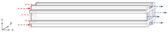
Figure 1.
Sketch of wall-flow filter model, consisting of one central inflow (red) channel with fractions of surrounding inflow and outflow (blue) channels separated by porous walls.
Within this model, a channel width of and a scaled channel length of is used. The latter accounts for a fifth of a real world representative of in order to achieve a reduction in computational load that enables the computationally demanding studies in the present work in the first place [11]. All pressure-related quantities in the present work can therefore be related to each other, but should not be considered for a quantitative comparison of their absolute value with those reported in different studies. The model’s general capability in recovering the correct pressure drop when considering a full-length channel could, however, be ensured by showing quantitative accordance with literature findings in Hafen et al. [9] and measurements on an experimental test rig in Hafen et al. [10]. The explicit influence of the gas temperature is not considered in this work and ambient conditions are assumed for the whole channel domain.
The model domain is spatially discretized with a resolution N that is defined as the number of cells per channel width . Periodic boundary conditions are then applied on the four surrounding sides, which let it serve as a representation of a real wall-flow filter comprised of hundreds of individual channels. Dirichlet boundary conditions [20] are used to impose a constant velocity at the inlets and a constant pressure at the outlets. No-slip conditions are assumed for the solid walls at the channel end caps on both sides. For the LBM-specific consideration, a simple bounce-back condition [23] is used for no-slip wall, regularized local boundary conditions [24] at the inlets and interpolated boundary conditions [25] at the outlets.
As the present work directly builds upon the results of its predecessor [11], a deposition layer during break-up due to the oxidization of the majority of its soot content [3] is considered as well. The individual layer fragments are modelled as a field of identical cubic discs that cover the porous walls inside an inflow channel. Here, a uniform field of fragments is considered as a base configuration on each of the four porous walls of the central inflow channel.
In order to avoid numerical instabilities from initially large gradients, all simulation runs are conducted by smoothly ramping up the inflow velocity to the prescribed one, while the fragments are artificially held in place. Afterwards, convergence of velocity, pressure and hydrodynamic force are evaluated in reoccurring steps in the whole fluid field analogously to [11]. Contrary to the previous work, however, simulations are not concluded when reaching a converged state, defined by the convergence criteria for velocity, pressure and hydrodynamic force. Instead, the fragments are released from their static state, which enables them to potentially detach and move through the channel when sufficient hydrodynamic forces are present. In order to retain reproducibility, no artificial randomness is considered either for the fragmented layer creation or during detachment. Due to the channel’s symmetry, this leads to the simultaneous detachment of multiple uniform fragments, which results in an accelerated rearrangement process with respect to a real-world counterpart. As reproducibility represents one of the prime advantages of simulations over experiments, this trade-off is chosen deliberately. A simulation is concluded when the cumulated kinetic energy over all fragments according to (5) falls below a predefined energy threshold. Every simulation run can accordingly be divided into four consecutive parts:
- Fluid velocity ramp-up and convergence with static fragmented layer;
- Detachment of fragments;
- Transport of fragments;
- Plug formation.
While the first one has been thoroughly investigated in the previous work, the present one focusses specifically on the last one. The conclusion of both periods is denoted fragmented layer state and plug state, respectively, and will be referenced throughout this work accordingly.
While such a rearrangement process may depend on many influence factors, the ones listed in Table 1 are investigated in this work.

Table 1.
Relevant quantities with base value and variation range considered in the respective investigations.
The first three factors cause modifications in the initial fragmented layer topology and the converged fluid field, respectively. They thus affect the complete rearrangement process. While the layer height depends on the loading time and PM concentration in the entering exhaust stream, the variation of fragment dimensions and the layer structure provides a simplified approach to account for the impact of the local distribution of ash and soot inside the PM layer. The latter four factors represent additional changes in PM properties and operating conditions, which impact the individual parts of a rearrangement process differently. The choice of base values and variation ranges results from a combined attempt to ensure stability, to keep the analogy to previous studies, to respect physical limitations and to maximize the sensitivity of the individual factors on the process.
In the previous work [11], an inflow velocity of and a resolution of was selected for all studies of a deposition layer during break-up. Due to the significantly increased computational demand resulting from the additional consideration of the transient effects, the present work adopts a smaller inflow velocity of , which enables a lower resolution of in order to avoid exceeding the available computational resources.
The discrete contact model, described in Section 2.1, requires the specification of respective material and mechanical properties. While those are in part subject to some uncertainty, they are kept constant in all studies to nonetheless ensure consistency throughout all investigations. For the porous substrate, a modulus of elasticity of and a Poisson’s ratio of can be assumed, following experimental measurements of Cordierite wall-flow filters [26,27]. Due to the lack of respective measurements for the PM under study, in this work, a Poisson’s ratio of is assumed for the PM layer fragments, adopting the properties of saturated clay [28]. It is worth noting at this point, however, that the effective modulus of elasticity in (2) exhibits a minor sensitivity to changes in the Poisson’s ratio of the fragments, owing to the large magnitudes associated with the moduli of elasticity in the denominators. Based on its minor stiffness, we assume a fragment’s modulus of elasticity of . Due to the contact model’s sensitivity to this parameter and the lack of existing data to substantiate this assumption, its impact is investigated as representative for the mechanical properties of PM as well (cf. Table 1). In order to ensure sufficient dissipation for the comparably coarse temporal resolution in the present work (), a coefficient of restitution of is used.
Analogous to the previous works [9,10,11,18], some relevant quantities are averaged at discrete locations over the cross-section of the central inlet channel and one representative outlet channel (denoted as and ) at recurring intervals and significant points in time. Next to the axial fluid velocity and the pressure p, this work now additionally considers the PM density , eventually providing a velocity, pressure and density profile , and along the channel length both at the converged fragmented layer state and the plug state. Such a density profile can then provide information about:
- Areas of complete detachment;
- Areas of incomplete detachment and re-deposition;
- Volume occupied by the plug;
- Local compactness inside the plug.
In order to enable a consistent quantification of the plug extent and its properties, a mean density profile is evaluated at the plug state. For this, the raw profile at plug state is smoothed by applying a Savitzky–Golay filter [29] with an order of 2 and a window size of 40 discrete points. The largest gradient in the smoothed profile is then interpreted as the transition point on the x-axis between layer and plug region. The original raw profile is averaged separately in both regions, yielding the mean density profile. This way, the plug starting position and its average density can be obtained as single-valued quantities, available for the comparison with other simulation. The individual steps are laid out at the first occurring of a density profile in Figure 7.
4. Results and Discussion
In the present section, the results from all simulation runs are presented, discussed and related to each other. First, the rearrangement process assuming the base configuration in Table 1 is evaluated in detail with respect to initial flow conditions in the converged state, the transient behaviour during rearrangement events and the final state in Section 4.1. Afterwards, the impact of influence factors that lead to a change in the fragmented layer topology on both the initial flow condition and the rearrangement process are laid out in Section 4.2. Additional PM properties and operating conditions that do not alter the initial state are then investigated in Section 4.3.
4.1. Rearrangement in Base Configuration
The base configuration represents the channel model with a fragmented deposition layer, assuming the exact values listed in Table 1. Its converged fragmented layer state (cf. Section 4.1.1), the following transient behaviour during rearrangement (cf. Section 4.1.2) and the final plug state are investigated separately in the following (cf. Section 4.1.3).
4.1.1. Fragmented Layer State
The flow field inside the channel including the fragmented layer at the converged state is shown in Figure 2.
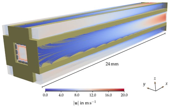
Figure 2.
Flow field with uniformly fragmented PM layer in gray. Dark yellow structures represent porous filter substrate, brown structures solid walls. Streamlines exhibit local flow direction. Colour scale indicates local velocity magnitude.
The flow field is represented by streamlines, which indicate the local flow direction and are coloured according to the local velocity magnitude. With those, the decrease in velocity magnitude inside the inlet channels can be identified over the channel length. A continuous magnitude increase can in turn be found in the outflow channels, eventually forming a developed channel profile at the outflow. As the fragmented deposition layer covers a large part of the central inlet channel’s cross-section, the area available for the flow is reduced, leading to significantly elevated velocities of up to with respect to the imposed average inflow velocity of .
The determination of the hydrodynamic forces acting on the particulate structures and the deduction of the local detachment likelihood of individual layer fragments, including their dependency on local flow conditions and the layer’s fragmentation, have been the subject of the predecessor work [11]. The corresponding velocity and pressure profiles and in the converged fragmented layer state can thus be found there, but have, additionally, been added as a reference to Figure 8.
4.1.2. Transient Behaviour
The transition from a uniformly fragmented deposition layer to an immobile plug configuration consists of detachment and transport of the individual fragments as well as the plug formation. The transient process in the central inlet channel is shown in Figure 3 at four exemplary points in time T1, T2, T3 and T4.
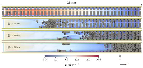
Figure 3.
Time series of detachment, transport and plug formation. Dark yellow structures represent porous filter substrate. Streamlines exhibit local flow direction. Colour scale indicates local velocity magnitude.
Time T1 represents the inner view of Figure 2, with the uniformly fragmented PM layer and a somewhat continuous layer of elevated fluid velocity closely above the fragmented layer over most of the channel length [11]. The fragments are then released (cf. Section 2), leading to a consecutive row-by-row detachment, which is caused by both increased flow exposition of initially shielded fragments and tear-off due to contact with suspended fragments flying by. This way, the number of simultaneously suspended fragments increases continuously until a major portion of the channel’s cross-section is occupied by them at T2. Due to the restored channel cross-section in the channel’s front, the local velocity magnitude decreases significantly here. At time T3, re-deposited fragments can be observed in the channel-mid, as fragment–fragment contact rather causes interception than tear-off due to the different flow conditions here. In a previous study on single fragment behaviour [10], fragments were found to always travel to the channel end once detached. When considering multi-fragment environments, this statement has to be extended with the possibility of interception, respectively. Time T4 shows the channel’s final state, where no fragments are suspended any more and a compact plug has formed at the channel end with a small region of undetachable fragments in front of it. Summing the kinetic energy in (5) over all individual layer fragments results in the cumulated kinetic energy , which provides a measure of the progress of the rearrangement process. Its temporal development is shown in Figure 4.
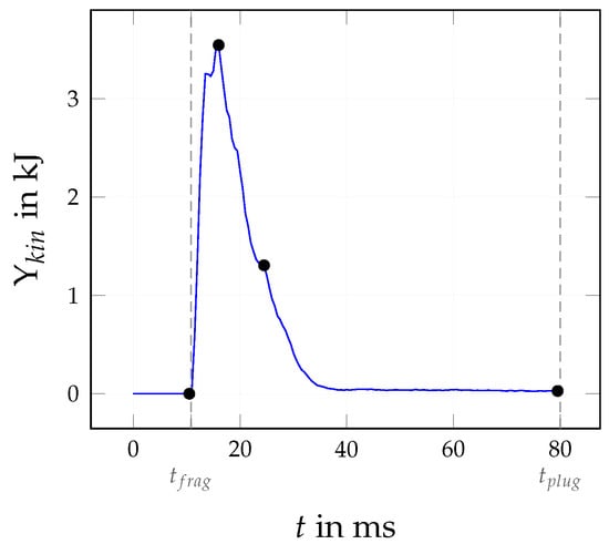
Figure 4.
Transient behaviour of fragments’ cumulated kinetic energy . Black dots represent relevant times in Figure 3. Dashed lines indicate time of converged fragmented layer state and final plug state .
The cumulated kinetic energy features a steep increase following the fragment’s release after fluid convergence, as fragments continuously detach and resuspend into the flow. A maximum is reached when the number of simultaneously suspended fragments is the highest and detaching fragments approximately equals those joining the plug formation or being intercepted mid-way. The cumulated kinetic energy then starts to decrease until reaching a level at around , where it approaches zero with a shallow slope. During this period, fragments steadily arrange inside the newly formed plug, whose compactness continuously increases. The transient development of the cumulated kinetic energy differs in part significantly throughout the different studies considered in this work. In order to ensure the comparability, a maximum simulation time of is identified as sufficient to capture all relevant transient effects in all simulation runs. That way, it simultaneously represents the time assumed for the evaluation of the plug state.
By averaging the discrete positions of all layer fragments, the average relative position of the total PM mass in the channel can be determined, which provides a simple single-valued measure for the spatial development during the rearrangement process. It can also provide some information about a continuing compaction, which reduces the channel volume occupied by the plug and may affect the total pressure drop. The temporal evolution of the relative average PM position and the pressure drop is shown in Figure 5.
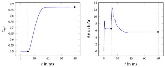
Figure 5.
Transient development of relative average PM position and pressure drop . Dashed lines indicate time of converged fragmented layer state and final plug state . Black dots represent sampling points at relevant states.
Due to its symmetry around the x-axis, a uniformly fragmented layer leads to an initial relative average PM position of . When the fragments are released after convergence and start to detach (cf. Section 3), the value increases steeply. The apparent smoothness of the course shows that the considered total number of fragments of can be reasoned to be statistically representative. After the first fragments hit the channel’s back wall, the slope decreases and starts to gradually approach a constant value, analogously to the cumulated kinetic energy in Figure 4.
The pressure drop, in turn, settles at a constant value of right after a start-up-induced fluctuation. When the fragments start to detach, the additional cross-section reduction observable at T2 in Figure 3 causes more flux to be redirected through the porous walls with an elevated wall-penetrating velocity. Here, the momentum loss increases, causing the pressure drop to rise as well. When the cross-section starts to clear up due to fewer particles detaching, the pressure starts decreasing again and continues to get smaller as more volume becomes available again for the flow. Analogously to the cumulated kinetic energy and the average PM position, the pressure drop then approaches a constant value. The resulting pressure drop of is smaller than the one at the converged layer state, with a difference of . This value is defined by the relation between an increase in the channel’s cross-section and the open flow area through the filter substrate on the one hand and a decrease in the available channel volume on the other hand. Both quantities in Figure 5 are sampled at the converged fragmented layer state and the final plug state for the comparison between different simulations in Section 4.2 and Section 4.3.
4.1.3. Plug State
The transient behaviour is concluded when reaching the plug state. A detailed view of the resulting plug packing is shown in Figure 6. All surfaces are coloured according to the magnitude of the local hydrodynamic force.
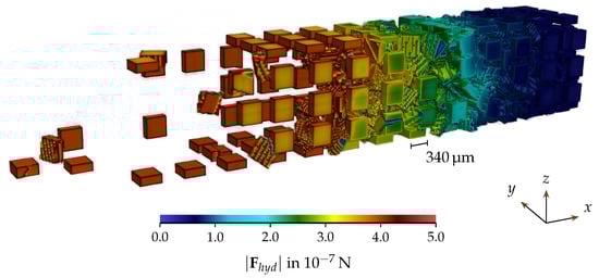
Figure 6.
Packing at plug state. Fragment surfaces coloured according to local contribution to hydrodynamic force magnitude . Porous substrate and flow removed for visual clarity.
It can be observed how the transported fragments form a dense packing over multiple fragment rows. Some undetached fragments can be found right in front of it, where the hydrodynamic forces in the normal direction of the substrate’s surface are not large enough to cause detachment. It also shows some redeposited particles, which have been intercepted during transport when loosing momentum due to contact with undetached fragments. The hydrodynamic force’s magnitude can be seen to decrease quickly when advancing further into the packing, indicating a continuously decreasing amount of fluid penetrating the plug. As the filter walls are permeable, they are subject to small currents inside them, causing a non-zero force contribution on each fragment’s bottom side.
The density profile for both fragmented layer and plug state is shown in Figure 7. The methodology for the evaluation of a mean density profile as described in Section 2 is outlined as well.
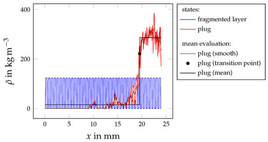
Figure 7.
PM density profile at fragmented layer and plug state. Additionally, layout of mean evaluation methodology according to Section 2.
It can be seen that the fragmented layer state is characterized by a non-negligible density which exhibits a periodic nature with a constant maximum, directly reflecting the PM layer height. The plug state, in turn, features a distinct profile, which shows no density in the frontal part of the channel, a small one in the channel-mid and a clearly identifiable plug region in the rear part of the channel beginning. The density reaches its maximum in the middle of the plug and decreases slightly both towards its front and the channel back wall.
The transition between layer and plug according to the mean density methodology lies at , which reveals that the plug occupies approximately of the central inflow channel’s volume at plug state. The resulting mean density profile (denoted in the following) exhibits an average plug density of , which lies well in the ranges of 220 to 330 [6] and 160 to 400 [16,17] reported in the literature for unsintered lube oil-derived ash.
The respective velocity and pressure profiles and in the central inlet channel and the representative outlet channel (cf. Section 3) are shown in Figure 8 for both fragmented layer and plug state.
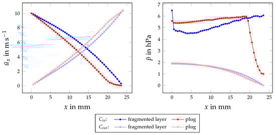
Figure 8.
Velocity profile and pressure profile in inlet channel domain and outlet channel domain at fragmented layer and plug state.
In the predecessor work [11], distinct profiles were identified in the fragmented layer state: The velocity is characterized by a transition from the imposed one to zero in the inflow channel domain and exhibits the opposite behaviour in the outflow channel domain . It should be noted at this point that all averaging is performed on the full channel cross-section. That way, an increase in the axial velocity due to a reduced area available for the flow does not impact the velocity profile, as fewer but higher velocities lead to the same average. It consequently represents a measure of the x-directed flux at a specific position. The pressure, however, decreases at a reduced available cross-section, as the velocity effectively increases. This results in a sudden pressure drop close to the inlet in the fragmented layer state. The pressure then gradually increases until reaching a local maximum near the back wall. The overall pressure level in the inflow channel results from the momentum loss due to the porous walls between the channels. In the outflow channel, in turn, the pressure decreases continuously with a decreasing slope, leading to a continuously increasing pressure difference between the inflow and outflow channel over its length. At the plug state, the velocity profile in the inflow channel changes significantly, as the rear part of the channel becomes occupied and the effective volume available for the flow decreases. As the flow resistance in the remaining part decreases additionally due to the increase in free substrate surface area, more fluid passes through the walls in the channel front and the mid-section. This becomes evident when considering the significantly decreased axial velocity in the inflow channel and the increased velocity over the whole length of the outflow channel. According to the observations made on Figure 7, the plug is not completely impenetrable, but rather exhibits a quickly decreasing permeability, which results in the observed continuously decreasing hydrodynamic surface force on the fragments. As derived from Figure 5, the pressure in the inlet decreases by at the plug state. Due to the complete detachment of the first fragment row, the sudden drop in pressure near the inlet vanishes. The profile then exhibits a shallow and nearly linear increase until reaching the plug’s beginning. Inside the plug, the pressure drops quickly to a level that lies even below the average outflow channel pressure.
4.2. Influence of Fragmented Layer Topology
In the following, the influence of the layer topology on the complete rearrangement process is investigated by considering differences in the layer height in Section 4.2.1, the fragment dimensions in Section 4.2.2 and the layer structure in Section 4.2.3. Next to quantitative evaluations, flow fields are shown for both the converged layer state and the final plug state.
4.2.1. Influence of Layer Height
A layer as thin as does not enable any detachment. The remaining range of considered PM layer heights in Table 1 is enclosed by the borderline cases and , for which the resulting flow field is shown in Figure 9 at the converged fragmented layer stage.
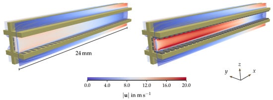
Figure 9.
Converged flow fields with uniformly fragmented PM layer in gray for layer heights (left) and (right) at fragmented layer state. Dark yellow structures represent porous filter substrate. Streamlines exhibit local flow direction. Colour scale indicates local velocity magnitude.
A direct comparison reveals large differences in the fluid velocity over the major part of the central inlet channel, as a cross-section reduction leads to significantly increased local and averaged axial fluid velocities. Those already hint at more fragment detachment due to an increased detachment likelihood [11] and faster fragment transport. The resulting flow fields at the final plug state are shown in Figure 10.
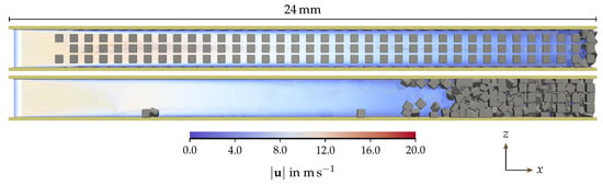
Figure 10.
Final flow fields with PM fragments in gray for layer heights (top) and (bottom) at plug state. Dark yellow structures represent porous filter substrate. Streamlines exhibit local flow direction. Colour scale indicates local velocity magnitude.
The formulated assumption can be confirmed, as detachment only occurred at the very first fragment rows for a layer height of , but over the whole channel length for a layer height of . The PM density profile and mean density profile (as laid out in Figure 7) are shown in Figure 11 for the considered range of layer heights.
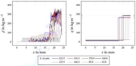
Figure 11.
PM density profile (left) and mean density profile (right) at plug state for different layer heights .
The profile exposes regions of different detachability: while for small layer heights, only the first few fragment rows detach, nearly complete detachment can be found for the largest height. The volume occupied by the resulting plug differs accordingly, as more detachment leads to more PM available for the plug formation, which gradually extends towards the inlet.
The dependency of the relative average PM position and the pressure drop on the layer height at both fragmented layer and plug state (cf. Figure 5) is laid out in Figure 12.
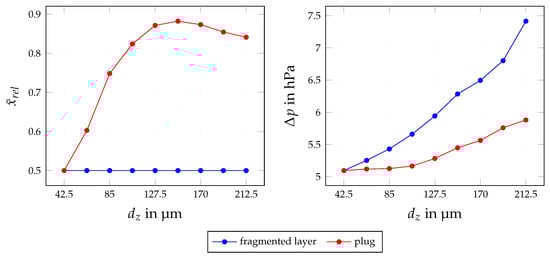
Figure 12.
Relative average PM position and pressure drop for different layer heights at fragmented layer and plug state.
As no detachment occurs for , both quantities are identical between the states. With increasing layer height, the relative average PM position then shifts towards the channel back at plug state due to the increasing number of detachable fragments. After reaching a maximum position of for , it decreases for larger layer heights as the plug continues to grow in a negative x-direction. Such a local maximum can consequently only be found for quantities that impact the detachment likelihood in a similarly pronounced way. The pressure drop increases continuously for both states, while exposing a much steeper slope at the fragmented state. This way, the difference becomes larger with increasing layer heights, with a maximum of for .
4.2.2. Influence of Fragment Dimensions
The flow fields for the lower and upper end of the considered fragment dimension range in Table 1 is shown in Figure 13.
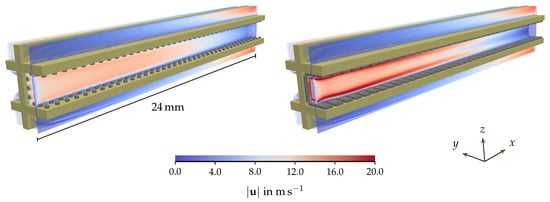
Figure 13.
Converged flow fields with uniformly fragmented PM layer in gray for fragment dimensions (left) and (right) at fragmented layer state. Dark yellow structures represent porous filter substrate. Streamlines exhibit local flow direction. Colour scale indicates local velocity magnitude.
Similarly to the relation in Figure 9, the larger fragment dimension leads to higher magnitudes of the fluid velocity due to the reduction in the channel’s cross-section. Additionally, the free surface area on the substrate is greatly reduced, which leads to an inhomogeneous velocity distribution of the channel cross-section with a pronounced layer of elevated fluid velocity closely above the fragmented layer. The resulting flow fields at the final plug state are shown in Figure 14.
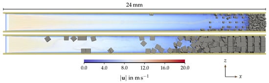
Figure 14.
Final flow fields with PM fragments in gray for fragment dimensions (top) and (bottom) at plug state. Dark yellow structures represent porous filter substrate. Streamlines exhibit local flow direction. Colour scale indicates local velocity magnitude.
Due to the large difference in available PM mass, the resulting plug size differs accordingly. For fragment dimensions of , a larger volume remains available for the flow. Complete detachment in the front and mid-section of the channel can be found in both cases, while the smaller fragment size exhibits an undetachable region in the additional flow volume due to insufficient axial flow velocities. The density profile for all considered fragment dimensions is shown in Figure 15.
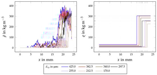
Figure 15.
PM density profile (left) and mean density profile (right) at plug state for different fragment dimensions .
Contrary to the observations made in Figure 11, no regions of undetachable fragments can be identified in the front and mid-section, even for small fragment dimensions. Detachability can consequently be assumed to feature a negligible sensitivity to the fragment dimensions in the considered range. Larger fragments, however, seem to be associated with a higher likelihood for interception during the transport, as non-zero density values reach further towards the inlet at the plug state. Inside the plug, differences are similar to those observed for the layer height, as the cumulated mass, hence the mean density, increases in both cases with larger fragments. The dependency of the relative average PM position and the pressure drop on the fragment dimensions at both states is shown in Figure 16.
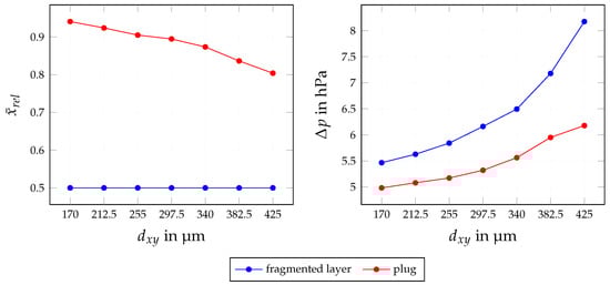
Figure 16.
Relative average PM position and pressure drop for different fragment dimensions at fragmented layer and plug state.
Contrary to a variation of the layer height in Figure 12 the average PM position continuously decreases with increasing fragment dimension. Due to negligible differences in the detachability, no inflection point can be found here and the average PM position directly reveals how far the plug reaches into the channel. The pressure increases for both states, with the difference between them continuously becoming larger. A fragment size of eventually results in a difference of .
4.2.3. Influence of Layer Structure
Depending on the amount and nature of inhomogeneities in the local distribution of reactive (soot) and inert (ash) components in a PM layer, a fragmentation due to the oxidation of the reactive components can lead to different amounts of equally sized PM fragments [3]. The borderline cases for the resulting layer structures are displayed in Figure 17.
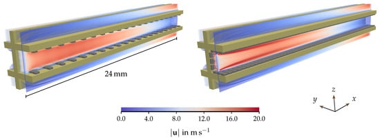
Figure 17.
Converged flow fields with uniformly fragmented PM layer in gray for numbers of fragment rows (left) and (right) at fragmented layer state. Dark yellow structures represent porous filter substrate. Streamlines exhibit local flow direction. Colour scale indicates local velocity magnitude.
While the cross-section at the position of fragment rows remains identical, the free surface area on the porous substrate differs significantly. Analogously to the observations in Figure 13, a reduction in free surface area leads to the development of a more inhomogeneous velocity distribution over the channel’s cross-section. A layer structure of shows the trailing fluid structures observed in Hafen et al. [11] behind each fragment row due to the large distance to the next one. When considering , in turn, each fragment row is shielded from the flow by the surrounding ones.
At plug state, the two borderline cases yield the flow fields shown in Figure 18.
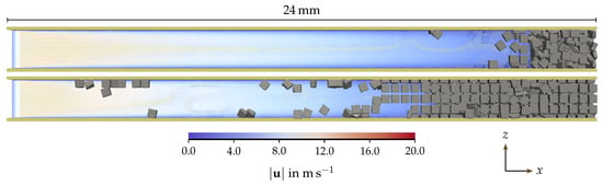
Figure 18.
Final flow fields with PM fragments in gray for numbers of fragment rows (top) and (bottom) at plug state. Dark yellow structures represent porous filter substrate. Streamlines exhibit local flow direction. Colour scale indicates local velocity magnitude.
The plug size, again, directly reflects the difference in available PM mass. The influence of the layer structure on the density profiles is shown in Figure 19.
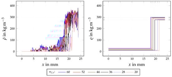
Figure 19.
PM density profile (left) and mean density profile (right) at plug state for different numbers of fragment rows .
It shows similar tendencies as the fragment dimension in Figure 15: Full detachment can be found for all variations in the channel’s front and mid-section. Solely a small section right in front of the plug shows a reduced detachability for a greater number of fragment rows due to the reduced exposition to the hydrodynamic forces at this position. Contrary to the influence of the fragment dimensions, the plug’s mean density exhibits a smaller sensitivity.
The relative average PM position in Figure 20 directly reflects the cumulated PM mass provided at the fragmented layer state, as it depicts plug growth towards the inlet. This growth leads to a nearly linear increase in the pressure drop at plug state. The pressure drop at the fragmented layer state exhibits a steeper slope and rises to larger values when the free substrate surface area becomes smaller. This rise eventually leads to a pressure drop difference of at between both states.
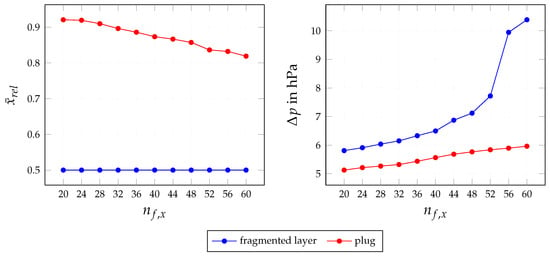
Figure 20.
Relative average PM position and pressure drop for different numbers of fragment rows at fragmented layer and plug state.
Some intermediate conclusions can be drawn from the investigation of all three topology variations, which can be attributed to two major causes: Firstly, the total PM mass present in the channel. As no continuing soot oxidization is considered, this mass stays constant throughout each simulation. Secondly, the free substrate surface area available for the flow at fragmented layer state. A reduction in this area leads to an inhomogeneity in the velocity distribution over the channel’s cross-section, which includes the development of a layer of elevated velocities closely above the fragments. This potentially leads to larger hydrodynamic forces on the deposited fragments and less propulsion in the channel’s centre during transport. In general, it can be stated that the topology at the fragmented layer state affects the final plug structure, while the impact on the pressure drop is smaller at plug state. The pressured dependency at plug state shows a more linear behaviour than the part super-linearly increasing fragmented layer state with potential jumps (cf. Figure 20). More specifically, larger layer heights, which represent longer loading times or higher PM concentrations, lead to greater pressure drops at plug state and an increased difference between both states. Larger fragment dimensions, associated with a smaller soot-to-ash ratio, lead to the same result. The more fragments remain after the soot oxidization, the larger the final pressure drop, with a pressure jump at and a substrate surface coverage of approximately . For a given PM mass present in the channel, the transition towards a plug becomes especially beneficial for the pressure drop when the fragmented PM layer only provides a small free substrate surface area available for the flow.
4.3. Influence of PM Properties and Operating Conditions
In addition to the investigation of the layer topology’s influence, the four remaining factors in Table 1, which do not alter the fragmented layer state, are considered in the following. Those include the PM density in Section 4.3.1, the fragments’ mechanical properties in Section 4.3.2, the adhesion between fragments and the porous substrate in Section 4.3.3 and the inflow velocity in Section 4.3.4.
4.3.1. Influence of PM Density
As a variation in the PM density represents a change in the fragment’s properties that eventually join the plug formation, the plug’s average density directly depends on the prescribed one. The volume occupied by the plug shows a non-negligible sensitivity, as it slightly grows with decreasing PM density (c.f. Figure 21). Due to the fact that the PM density neither impacts the hydrodynamic surface force nor the contact forces in (1), it only affects a fragment’s inertia, which is solely relevant for the detachment and transport process. Fragments with higher densities accordingly hit an existing plug structure with more momentum, causing a small compaction. Such a compaction can clearly be identified in the behaviour of the relative average PM position in Figure 22.
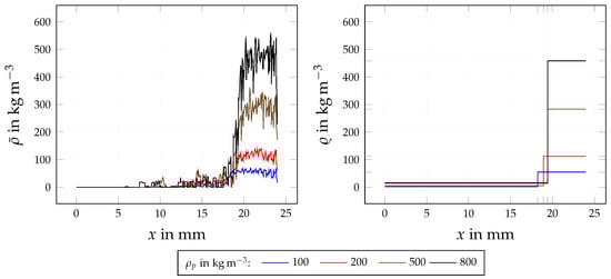
Figure 21.
PM density profile (left) and mean density profile (right) at plug state for different PM densities .
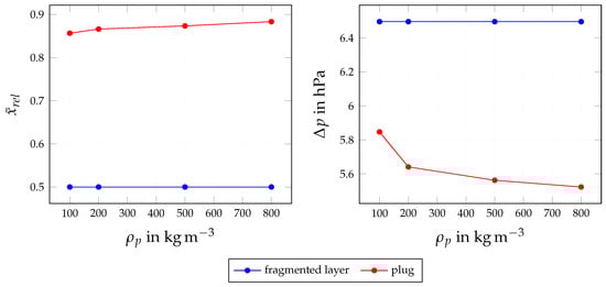
Figure 22.
Relative average PM position and pressure drop for different PM densities at fragmented layer and plug state.
The pressure drop at plug state decreases respectively with decreasing plug volume. A larger PM density, therefore, leads to a smaller pressure drop at plug state due to the formation of a more compact plug as a result of higher inertia.
4.3.2. Influence of Mechanical Properties
The fragments’ mechanical properties neither affect the fragmented layer state nor the detachment process. While not directly impacting the transport either, any contact with the substrate wall or other fragments on their way can cause a change in trajectory or velocity. The density profile in Figure 23 therefore exhibits no distinct difference in the detachability.
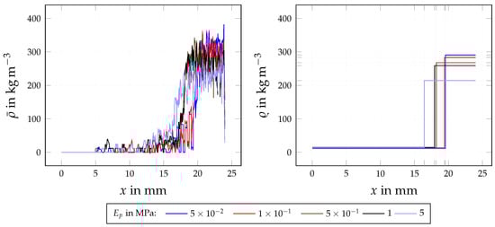
Figure 23.
PM density profile (left) and mean density profile (right) at plug state for different fragment moduli of elasticity .
It can be observed that a large elasticity of leads to an increase in the plug volume, as repulsion forces become larger at fragment–fragment contacts according to (1) and counteract further compaction. As the density inside the plug becomes smaller for those as well, the plug’s porosity increases additionally. The relative average PM position in Figure 24 directly reflects the volume increase due to the less compact packing.
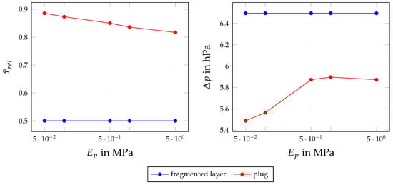
Figure 24.
Relative average PM position and pressure drop for different fragment moduli of elasticity at fragmented layer and plug state.
The pressure drop at plug state initially increases with the plug volume. It then transitions into a nearly constant value of at due to the continuous increase in the plug’s porosity, which compensates for the reduced volume available for the flow. The results suggest that using additives, which decrease the fragments’ stiffness, would be beneficial for the reduction in the pressure drop due to a more compact plug.
4.3.3. Influence of Adhesive Forces
According to the studies conducted in Hafen et al. [11], detachment of the fragments in the first row is assisted by a hydrodynamic force of assuming an inflow velocity of . As the acting forces are significantly smaller for all other rows, no detachment occurs with adhesion forces in normal direction of the substrate’s surface of or larger present. For the remaining range of considered adhesion forces in Table 1, the density profile is shown in Figure 25.
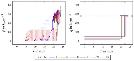
Figure 25.
PM density profile (left) and mean density profile (right) at plug state for different adhesive forces .
As predicted by the detachment likelihood formulated in Hafen et al. [11], the fragment rows closest to the inlet detach first when reducing the adhesion force to . With a continuous adhesion reduction, more neighbouring fragment rows become detachable. While the plug volume stays similar for higher values, it increases for . Thus, the relative average PM position in Figure 26 can at smaller adhesive forces be attributed to the plug volume only. At larger ones, it then reflects regions of partial detachment and fragment interception, similarly to findings in Figure 12 between and .
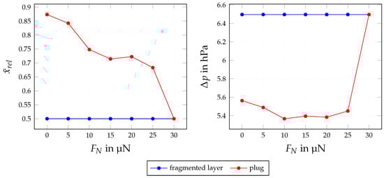
Figure 26.
Relative average PM position and pressure drop for different adhesive forces at fragmented layer and plug state.
The pressure drop at the plug state revolves around a small range between 5.40 hPa and 5.59 hPa and stays nearly constant for adhesion forces of , which corresponds to the observed similar plug volume. For smaller adhesion forces, the pressure drop increases slightly due to the increased plug volume. It becomes clear that the removal of the first few fragment rows already causes the major part of the pressure drop reduction with respect to the fragmented layer state. Additionally, it can be observed that adhesive forces are only relevant around the detachment threshold of the first fragment row, as a further reduction has a negligible influence on the detachment and the pressure drop accordingly.
4.3.4. Influence of Inflow Velocity
The inflow velocity is directly responsible for the magnitude of the hydrodynamic forces present in the channel. It accordingly impacts the fragmented layer state, the detachment process, the pneumatic transport and the plug formation. A velocity of shows a significant number of undetachable fragments in Figure 27.
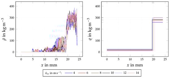
Figure 27.
PM density profile (left) and mean density profile (right) at plug state for different inflow velocities .
For higher inflow velocities, the plug’s density profile exhibits a very similar structure, with small differences in the plug’s mean density. The relative average PM position in Figure 28 does not show a large sensitivity on the inflow velocity either.
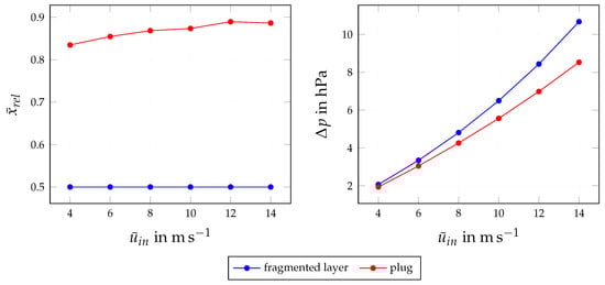
Figure 28.
Relative average PM position and pressure drop for different inflow velocities at fragmented layer and plug state.
A slight increase is caused by the continuously increasing inertia of fragments hitting the plug and causing a compaction similarly to the observations in Figure 22. At smaller velocities, this effect is superimposed by the increasing number of detachable fragments. As a result of an increased momentum loss due to a higher wall through-put, the pressure drop shows a strong sensitivity to the inflow velocity for both states. While the plug state exhibits a nearly linear profile, the fragmented layer state increases super-linearly, leading to a continuously growing difference between both states until reaching at . In comparison with the strong relation between gas velocity and momentum loss in the filter substrate, however, the superposed pressure drop dependency at plug state proves to be less relevant.
5. Conclusions
In this work, the dynamic rearrangement process during the regeneration of a wall-flow filter channel was investigated using the open source software OpenLB [12,13]. As a direct sequel to the investigation of the static fragmented layer exposed to elevated fluid velocities in Hafen et al. [11], the present work additionally investigated the dynamic behaviour during fragment detachment, fragment transport and plug formation. First, the complete rearrangement process was evaluated in detail, considering a constant base configuration for the influence factors (cf. Section 4.1). With it, it could be shown that fragments detach row-by-row, confirming the assumption of the predecessor work. Fragment–fragment contact in the channel’s front turned out to potentially cause tear-off, while it causes interception in the channel-mid. The inclusion of the discrete contact model proved to enable the successful formation of an end plug occupying a significant amount of the available channel volume. A simple mean density methodology was presented and could be shown to represent a reproducible way of determining the plug extent and its average density, which agrees well with values reported by Kimura et al. [16], Sappok et al. [17] and Dittler [6]. Afterwards, the impact of influence factors that lead to a change in the fragmented layer topology on both the initial flow condition and the rearrangement process were laid out (cf. Section 4.2). While the topology of the fragmented layer could be shown to affect the final plug structure, its pressure drop impact on the initial fragmented layer state was identified to be greater. Larger layer heights, which represent longer loading times or higher PM concentrations, could be shown to lead to greater pressure drops at plug state and an increased difference between both states. Larger fragment dimensions, associated with a smaller soot-to-ash ratio, were shown to lead to the same result. It turned out that a larger number of fragments remaining after the soot oxidization leads to a larger final pressure drop. For a given mass of PM present in the channel, the transition towards a PM plug was shown to be especially beneficial when the fragmented layer only provides a small free substrate surface area available for the flow. Lastly, additional PM properties and operating condition that do not alter the initial fragmented layer topology were investigated (cf. Section 4.3). A larger PM density could be shown to lead to a smaller pressure drop at plug state due to the formation of a more compact plug as a result of higher fragment inertia. It was reasoned that the use of additives, which decrease the fragments’ stiffness, would be beneficial for the reduction in the pressure drop due to a more compact plug. It could be shown that the removal of the first few fragment rows already causes the major part of the pressure drop reduction with respect to the fragmented layer state. Additionally, it could be shown that adhesive forces are only relevant around the detachment threshold of the first fragment row, as a further reduction has a negligible influence on the detachment and the pressure drop accordingly. In comparison with the strong relation between gas velocity and momentum loss in the filter substrate, the superposed pressure drop dependency at plug state was identified as less relevant.
While not attempting a systematic comparison of the different influence factors with each other, it can be argued that the inflow velocity (cf. Section 4.3.4) and the layer structure (cf. Section 4.2.3) have the largest impact on the final pressure drop. They can, accordingly, be designated as the most crucial ones for the dynamic rearrangement process in wall-flow filters.
The present work demonstrated the successful extension of the resolved particle methodology via a discrete method to treat particle–particle and particle–wall interactions and its application to the transient rearrangement process in wall-flow filters. Additionally, it reveals the sensitivity of relevant influence factors related to the fragmented layer topology, the PM properties and the operating conditions, and quantifies their impact on the rearrangement process. This way, it contributes to the formulation of respective predictions on the deposition pattern formation, which impact engine performance, fuel consumption and service life of wall-flow filters.
Author Contributions
Conceptualization, N.H., A.D. and M.J.K.; methodology, N.H., J.E.M., A.D. and M.J.K.; software, N.H., J.E.M. and M.J.K.; validation, N.H.; formal analysis, N.H., J.E.M., A.D. and M.J.K.; investigation, N.H.; resources, A.D. and M.J.K.; data curation, N.H.; writing—original draft preparation, N.H.; writing—review and editing, N.H., J.E.M., A.D. and M.J.K.; visualization, N.H.; supervision, A.D. and M.J.K.; project administration, N.H., A.D. and M.J.K.; funding acquisition, N.H., A.D. and M.J.K. All authors have read and agreed to the published version of the manuscript.
Funding
Funded by the Deutsche Forschungsgemeinschaft (DFG, German Research Foundation)—422374351.
Data Availability Statement
Not applicable.
Acknowledgments
We acknowledge support by the KIT-Publication Fund of the Karlsruhe Institute of Technology. This work was performed on the HoreKa supercomputer funded by the Ministry of Science, Research and the Arts Baden-Württemberg and by the Federal Ministry of Education and Research.
Conflicts of Interest
The authors declare no conflict of interest.
Abbreviations
The following abbreviations are used in this manuscript:
| CFD | computational fluid dynamics |
| LBM | lattice Boltzmann method |
| NSE | Navier–Stokes equation |
| PM | particulate matter |
Nomenclature
The following symbols are used in this manuscript:
| fluid velocity | |
| p | fluid pressure |
| position | |
| t | time |
| N | resolution of voxel mesh |
| particle velocity | |
| particle angular velocity | |
| particle mass | |
| particle’s momentum of inertia | |
| particle’s kinetic energy | |
| channel length | |
| channel width | |
| scaled channel length | |
| average inflow velocity | |
| particle density | |
| mean density (along layer and plug) | |
| fragment’s x-dimension | |
| fragment’s equilateral width | |
| hydrodynamic normal force | |
| number of fragment rows over channel length | |
| time at converged fragmented layer state | |
| time at final plug state | |
| Inlet channel domain | |
| Outlet channel domain | |
| normal contact force | |
| effective modulus of elasticity | |
| k | contact type constant |
| contact overlap volume | |
| contact indentation depth | |
| c | damping factor |
| relative velocity between objects | |
| modulus of elasticity of object A | |
| Poisson’s ratio of object A | |
| e | coefficient of restitution |
| domain of central inlet channel | |
| domain of representative outlet channel |
References
- Wang, Y.; Kamp, C.J.; Wang, Y.; Toops, T.J.; Su, C.; Wang, R.; Gong, J.; Wong, V.W. The origin, transport and evolution of ash in engine particulate filters. Appl. Energy 2020, 263, 114631. [Google Scholar] [CrossRef]
- Gaiser, G. Berechnung von Druckverlust, Ruß- und Ascheverteilung in Partikelfiltern. MTZ-Mot. Z. 2005, 66, 92–102. [Google Scholar] [CrossRef]
- Sappok, A.; Govani, I.; Kamp, C.; Wang, Y.; Wong, V. In-Situ Optical Analysis of Ash Formation and Transport in Diesel Particulate Filters during Active and Passive DPF Regeneration Processes. SAE Int. J. Fuels Lubr. 2013, 6, 336–349. [Google Scholar] [CrossRef]
- Ishizawa, T.; Yamane, H.; Satoh, H.; Sekiguchi, K.; Arai, M.; Yoshimoto, N.; Inoue, T. Investigation into Ash Loading and Its Relationship to DPF Regeneration Method. SAE Int. J. Commer. Veh. 2009, 2, 164–175. [Google Scholar] [CrossRef]
- Aravelli, K.; Heibel, A. Improved Lifetime Pressure Drop Management for Robust Cordierite (RC) Filters with Asymmetric Cell Technology (ACT). In Proceedings of the SAE World Congress & Exhibition; SAE International: Warrendale, PA, USA, 2007. [Google Scholar] [CrossRef]
- Dittler, A. Ash Transport in Diesel Particle Filters. In Proceedings of the SAE 2012 International Powertrains, Fuels & Lubricants Meeting; SAE International: Warrendale, PA, USA, 2012. [Google Scholar] [CrossRef]
- Dittler, A. Abgasnachbehandlung mit Partikelfiltersystemen in Nutzfahrzeugen, 1st ed.; Wuppertaler Reihe zur Umweltsicherheit; Shaker: Herzogenrath, Germany, 2014. [Google Scholar]
- Wang, Y.; Kamp, C. The Effects of Mid-Channel Ash Plug on DPF Pressure Drop. In Proceedings of the SAE 2016 World Congress and Exhibition; SAE International: Warrendale, PA, USA, 2016. [Google Scholar] [CrossRef]
- Hafen, N.; Dittler, A.; Krause, M.J. Simulation of particulate matter structure detachment from surfaces of wall-flow filters applying lattice Boltzmann methods. Comput. Fluids 2022, 239, 105381. [Google Scholar] [CrossRef]
- Hafen, N.; Thieringer, J.R.; Meyer, J.; Krause, M.J.; Dittler, A. Numerical investigation of detachment and transport of particulate structures in wall-flow filters using lattice Boltzmann methods. J. Fluid Mech. 2023, 956, A30. [Google Scholar] [CrossRef]
- Hafen, N.; Marquardt, J.E.; Dittler, A.; Krause, M.J. Simulation of Particulate Matter Structure Detachment from Surfaces of Wall-Flow Filters for Elevated Velocities Applying Lattice Boltzmann Methods. Fluids 2023, 8, 99. [Google Scholar] [CrossRef]
- Krause, M.J.; Kummerländer, A.; Avis, S.J.; Kusumaatmaja, H.; Dapelo, D.; Klemens, F.; Gaedtke, M.; Hafen, N.; Mink, A.; Trunk, R.; et al. OpenLB—Open source lattice Boltzmann code. Comput. Math. Appl. 2021, 81, 258–288. [Google Scholar] [CrossRef]
- Kummerländer, A.; Avis, S.; Kusumaatmaja, H.; Bukreev, F.; Crocoll, M.; Dapelo, D.; Hafen, N.; Ito, S.; Jeßberger, J.; Marquardt, J.E.; et al. OpenLB Release 1.6: Open Source Lattice Boltzmann Code. 2023. Available online: https://doi.org/10.5281/zenodo.7773497 (accessed on 18 June 2023).
- Konstandopoulos, A.G.; Skaperdas, E.; Warren, J.; Allansson, R. Optimized Filter Design and Selection Criteria for Continuously Regenerating Diesel Particulate Traps. In Proceedings of the International Congress & Exposition; SAE International: Warrendale, PA, USA, 1999. [Google Scholar] [CrossRef]
- Thieringer, J.R.D.; Hafen, N.; Meyer, J.; Krause, M.J.; Dittler, A. Investigation of the Rearrangement of Reactive ash; Inert Particulate Structures in a Single Channel of a Wall-Flow Filter. Separations 2022, 9, 195. [Google Scholar] [CrossRef]
- Kimura, K.; Lynskey, M.; Corrigan, E.R.; Hickman, D.L.; Wang, J.; Fang, H.L.; Chatterjee, S. Real World Study of Diesel Particulate Filter Ash Accumulation in Heavy-Duty Diesel Trucks. In Proceedings of the Powertrain & Fluid Systems Conference and Exhibition; SAE International: Warrendale, PA, USA, 2006. [Google Scholar] [CrossRef]
- Sappok, A.; Santiago, M.; Vianna, T.; Wong, V.W. Controlled Experiments on the Effects of Lubricant/Additive (Low-Ash, Ashless) Characteristics on DPF Degradation. In Proceedings of the Diesel Engine-Efficiency and Emissions Research (DEER) Conference, Dearborn, MI, USA, 4–7 August 2008. [Google Scholar]
- Hafen, N.; Krause, M.J.; Dittler, A. Simulation of Particle-Agglomerate Transport in a Particle Filter using Lattice Boltzmann Methods. In 22. Internationales Stuttgarter Symposium; Bargende, M., Reuss, H.C., Wagner, A., Eds.; Springer: Wiesbaden, Germany, 2022; pp. 292–303. [Google Scholar]
- Marquardt, J.E.; Römer, U.J.; Nirschl, H.; Krause, M.J. A discrete contact model for complex arbitrary-shaped convex geometries. Particuology 2023, 80, 180–191. [Google Scholar] [CrossRef]
- Ferziger, J.H.; Perić, M. Numerische Strömungsmechanik; Springer eBook Collection; Springer: Berlin/Heidelberg, Germany, 2008. [Google Scholar] [CrossRef]
- Nassauer, B.; Kuna, M. Contact forces of polyhedral particles in discrete element method. Granul. Matter 2013, 15, 349–355. [Google Scholar] [CrossRef]
- Carvalho, A.S.; Martins, J.M. Exact restitution and generalizations for the Hunt–Crossley contact model. Mech. Mach. Theory 2019, 139, 174–194. [Google Scholar] [CrossRef]
- Ladd, A.J.C. Numerical simulations of particulate suspensions via a discretized Boltzmann equation. Part 1. Theoretical foundation. J. Fluid Mech. 1994, 271, 285–309. [Google Scholar] [CrossRef]
- Latt, J.; Chopard, B.; Malaspinas, O.; Deville, M.; Michler, A. Straight velocity boundaries in the lattice Boltzmann method. Phys. Rev. E 2008, 77, 056703. [Google Scholar] [CrossRef] [PubMed]
- Skordos, P.A. Initial and boundary conditions for the lattice Boltzmann method. Phys. Rev. E 1993, 48, 4823–4842. [Google Scholar] [CrossRef]
- Cooper, R.C.; Bruno, G.; Onel, Y.; Lange, A.; Watkins, T.R.; Shyam, A. Young’s modulus and Poisson’s ratio changes due to machining in porous microcracked cordierite. J. Mater. Sci. 2016, 51, 9749–9760. [Google Scholar] [CrossRef]
- Pandey, A.; Shyam, A.; Watkins, T.R.; Lara-Curzio, E.; Stafford, R.J.; Hemker, K.J. The Uniaxial Tensile Response of Porous and Microcracked Ceramic Materials. J. Am. Ceram. Soc. 2014, 97, 899–906. [Google Scholar] [CrossRef]
- Thota, S.K.; Cao, T.D.; Vahedifard, F. Poissons Ratio Characteristic Curve of Unsaturated Soils. J. Geotech. Geoenviron. Eng. 2021, 147, 04020149. [Google Scholar] [CrossRef]
- Savitzky, A.; Golay, M.J.E. Smoothing and differentiation of data by simplified least squares procedures. Anal. Chem. 1964, 36, 1627–1639. [Google Scholar] [CrossRef]


Disclaimer/Publisher’s Note: The statements, opinions and data contained in all publications are solely those of the individual author(s) and contributor(s) and not of MDPI and/or the editor(s). MDPI and/or the editor(s) disclaim responsibility for any injury to people or property resulting from any ideas, methods, instructions or products referred to in the content. |
© 2023 by the authors. Licensee MDPI, Basel, Switzerland. This article is an open access article distributed under the terms and conditions of the Creative Commons Attribution (CC BY) license (https://creativecommons.org/licenses/by/4.0/).