Abstract
It is well established that spray characteristics from automotive injectors depend on, among other factors, whether cavitation arises in the injector nozzle. Bulk cavitation, which refers to the cavitation development distant from walls and thus far from the streamline curvature associated with salient points on a wall, has not been thoroughly investigated experimentally in injector nozzles. Consequently, it is not clear what is causing this phenomenon. The research objective of this study was to visualize cavitation in three different injector models (designated as Type A, Type B, and Type C) and quantify the liquid flow field in relation to the bulk cavitation phenomenon. In all models, bulk cavitation was present. We expected this bulk cavitation to be associated with a swirling flow with its axis parallel to that of the nozzle. However, liquid velocity measurements obtained through particle image velocimetry (PIV) demonstrated the absence of a swirling flow structure in the mean flow field just upstream of the nozzle exit, at a plane normal to the hypothetical axis of the injector. Consequently, we applied proper orthogonal decomposition (POD) to analyze the instantaneous liquid velocity data records in order to capture the dominant coherent structures potentially related to cavitation. It was found that the most energetic mode of the liquid flow field corresponded to the expected instantaneous swirling flow structure when bulk cavitation was present in the flow.
1. Introduction
Cavitation is an important factor for spray formation within diesel or gasoline injectors, and it appears to affect the properties of the resultant spray [1,2]. In addition, differences in the spray cone angle and tip penetration have been reported in [3,4,5,6] depending on the type of cavitation observed (with edge flow separation cavitation occurring close to the walls or bulk cavitation, which occurs within the flow far from the walls). While the potential role of edge flow separation cavitation on spray formation in nozzles has been thoroughly investigated, the formation and the effects of bulk cavitation are issues that need more attention in terms of acquiring quantitative flow field data. The phenomenon of bulk cavitation (or string cavitation) has been reported in diesel model injectors in references [7,8,9], as well as in gasoline injectors in references [10,11,12]. Recent studies on the visualization of string cavitation have attempted to explain the interaction of vortices between adjacent nozzles when bulk cavitation is present in diesel multi-hole injectors [13]. Additionally, these studies have explored the temporal evolution of this type of cavitation and the cycle-by-cycle variation in its shape [14]. However, neither study has provided quantitative flow field data for the bulk cavitation area. Only in [15] were some flow field data derived through a simulation based on the work of [16] provided. These simulations showed the presence of a vortical flow around the core of bulk cavitation.
Based on computational pressure field results, it has also been suggested that the initiation of this type of cavitation is a result of gas-phase components that remain after previous injection events, with vortices acting as gas-phase carriers. These studies have provided valuable insight into this phenomenon. However, to our knowledge, computational fluid mechanic tools for calculating the flow field in relation to bulk cavitation, as presented in reference [16] and other computational studies ([17,18,19]), are not (yet) capable of predicting bulk cavitation. Whether it is vortex-induced cavitation or the elongated bubble clouds of the remaining gas phase, this phenomenon influences the surrounding flow field and, more specifically, leads to the redistribution of vorticity, as mentioned in reference [20]. In addition, it has been reported in reference [21] that vortex properties determine the dynamics (growth and collapse) and shape of bulk cavitation. This, along with the fact that bulk cavitation can affect spray properties, motivated our targeted flow field measurements to correlate with this phenomenon.
Reports on the flow field inside injectors, which could be responsible for the formation of bulk cavitation, are limited. An early reference providing quantitative PIV measurements inside diesel fuel injectors was reported in reference [22], followed by the laser Doppler velocimetry measurements (LDV) presented in reference [23]. PIV measurements on the internal flow field of fuel injectors are also presented in references [12,24,25,26]. In the last reference, the authors observed the presence of bulk cavitation in the same injector geometries as those examined in this paper. In a recent publication [4], 2D PIV was applied to a full-size diesel injector in the area just upstream of the nozzle exit, where bulk cavitation was initiated. However, although some vortical structures seemed to be present, detailed high-resolution experimental flow field data that could quantify the presence of vortices in that area were not provided. Finally, the study presented in references [27,28,29] experimentally demonstrated in model nozzles that downstream of the flow separation cavitation occurring at the nozzle entry, instantaneous vortices are initiated in the shear layer of the liquid flow. These vortices can lead to a low enough local pressure to cause bulk cavitation, which even extends into the liquid container attached downstream from the nozzle exit. However, the authors did not quantify the local velocity field associated with these structures. Therefore, the literature indicates that the local flow field may be able to induce bulk cavitation.
As a continuation of the work reported in reference [12], bulk cavitation was visualized in three gasoline multi-hole injectors. A two-dimensional micron resolution particle imaging velocimetry was employed to measure the internal flow field of 10:1 super-scale transparent models of multi-hole injectors in the vicinity of a region just upstream from the entrance to the holes of the injector plates, under conditions shortly after the onset of cavitation. This plane of measurement was parallel to the injector plates (which is normal to the notional axis of symmetry in the injector). In cases where bulk cavitation was present, we applied proper orthogonal decomposition (POD) to the measured instantaneous velocity data in order to capture the dominant coherent structures potentially related to cavitation. Our objective was not only to visualize cavitation but also to correlate the flow field upstream of the nozzles with the occurrence of bulk cavitation within the nozzles. In addition, the probability of bulk cavitation was calculated by applying POD to shadowgraph images of different nozzles of the same type of injector. Details of the experimental techniques and methods used are provided in the next section. Subsequently, the results are presented, and the paper concludes with a summary of the main findings.
2. Experimental Methods and Analysis
2.1. Injector Models, Experimental Setup, and Measurement Conditions
The schematics of the gasoline injector models are shown in Figure 1 for Type A and B models and in Figure 2 for the Type C model. Details of the significant differences in geometry between Types A and C are briefly described below; these details can be found in [12]. The main parts of the injector model are shown, and the planes of measurement are indicated with the grey area, with one occupied by a refractive index matching liquid. These models, which are scaled up by a factor of 10, represent the parts of the prototype gasoline injectors, which are adjacent to the nozzles. The model was finished to the required optical surface quality (Kuwana Engineering Plastic Co., Ltd., Kuwana, Japan).
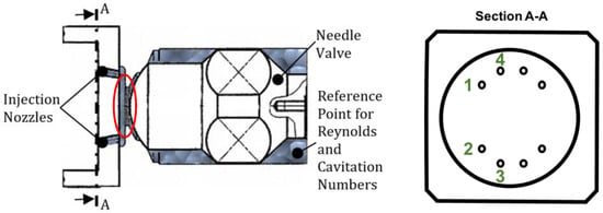
Figure 1.
(left) Schematic of Type A and Type B injector model. Grey area indicates fluid flow. Flow is from right to left. (right) Section A-A shows the nozzle arrangement. Numbers in green identify nozzle numbers 1–4, some of which are referred to in the ‘Results and Discussion’ section.
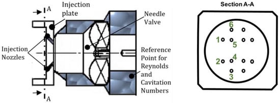
Figure 2.
(left) Schematic of Type C injector model. Grey area indicates fluid flow. Flow is from right to left. (right) Section A-A shows the nozzle arrangement. Numbers in green identify nozzle numbers 1–6, some of which are referred to in the ‘Results and Discussion’ section.
It should be noted that Types A and B injectors have 8 nozzles, and Type C has 12. The locations of the nozzles are indicated in the respective injection plate in Figure 1 and Figure 2. The differences in the geometry between Types A and B were minor, while for the case of Type C, the cylindrical sections were larger in diameter and, in combination with the needle valve geometry, led to more abrupt changes in the flow direction compared to the case of Type A model. In addition, in the Type C injector, the size of the holes is slightly smaller, and also, the distance between neighboring holes is smaller. The main difference between Type A and Type B is that, for the latter, the “neck” (see the encircled part in Figure 1) is longer. This was expected to induce differences in the hairpin type flow as the liquid enters the sections just upstream of the nozzles, which were validated with PIV, compared with the measurements shown in [25]. In terms of the needle valve, although the geometry is similar between Type A and Type B, the cylinder with the spherical valve end is shorter and has a larger diameter in the former. This allows shorter flow paths to the sections that include the above-mentioned part of the needle valve. The needle valve lift for all cases (Type A, B, and C) was set to 0.8 mm in the model, corresponding to the maximum needle valve lift of the prototype.
In all the model injectors, the flow is from right to left (refer to the grey area in Figure 1 and Figure 2). The flow is contained in the annular passage between the needle valve and the needle valve seat until the exit nozzles. The hydraulic circuit used, which contained a refractive index matching fluid (31.65% v/v of 1,2,3,4–Tetrahydronaphthalene and 68.35% v/v of turpentine oil), is illustrated in Figure 3. All the tubing was made of stainless steel in order to withstand the corrosive mixture of the working fluid, which was connected to the model with a reinforced plastic tube. There were two pumps that circulated the working fluid. Pump 1 was of low capacity (1.5 m3/h), and Pump 2 had a maximum flow rate of 8 m3/h. Pump 1 was used for low Reynolds Number conditions and Pump 2 for high Reynolds Numbers, which were near the conditions of the initiation of cavitation. It should be noted that the temperature of the liquid was continuously monitored by a thermocouple. A cooler controlled the temperature of the liquid at 25 °C with an accuracy of 0.1 °C. This was performed because the fluid’s refractive index was affected by temperature changes, and it only showed the desired refractive index (1.49, same as that of the acrylic plastic material of the model) at a temperature of 25 °C. Though not shown here and as explained in [12], downstream of the exit from the nozzles, the flow proceeded to a large liquid-filled plenum, from which it is redirected back to the liquid ‘sump’ tank: part of the hydraulic circuit. The outflow pattern was certainly affected by this setup, but it is not examined in this work, as only measurements from the internal flow field were acquired. Upstream of the injector body, the conditions of these measurements were set so that the internal flow could bear geometrical and dynamic similarity with the prototype injector.
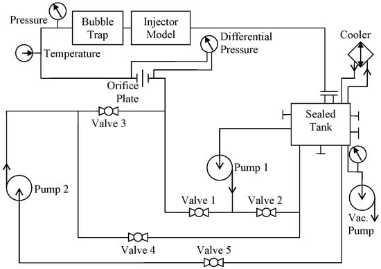
Figure 3.
Hydraulic circuit of the refractive index matching rig (Aleiferis et al. [26]).
A bubble trap was used to capture gas bubbles, which were physically trapped in the model and could be present in the working fluid, either during the filling of the hydraulic circuit or when dissolved in the liquid and after cavitation was initiated for some flow conditions. This was a settling chamber with the inlet at the top and the outlet at the bottom so that any bubbles could flow to the top part of the chamber. A schematic of the bubble trap is given in Figure 4. It should also be noted that the flow downstream of the nozzle exit was liquid, and there was no chance to entrain air from outside the nozzle. Therefore, the reported observations are only due to local cavitation in the flow. A vacuum pump acted on the free surface of the liquid downstream of the model in the sealed tank so that the downstream static pressure of the liquid was controlled in order for the cavitation number to be matched between the real and large-scale models above the pressure limits (0.2–0.4 atm depending on the pump in operation). This was allowed by the Net Positive Suction Head (NPSH) of each pump. If we applied a lower pressure than the NPSH of the pump, we could induce cavitation upstream of the injector model, which was not desirable. More details about the operation of the hydraulic circuit can be found in [25,26]. To investigate the temporal development of cavitation in all three different geometries, we used a high-speed camera, “KODAK HS 4500”, which had a frame rate of 4500 fps at a maximum resolution (256 pixels × 256 pixels), although velocities were not measured while acquiring high temporal resolution pictures because the available high resolution (2048 pixels × 2048 pixels) PIV system had a maximum acquisition frequency of 10 Hz.
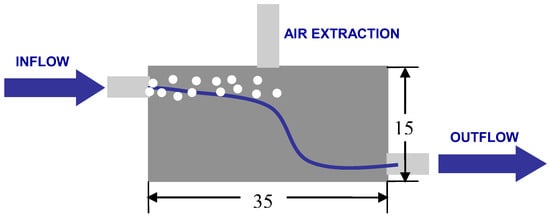
Figure 4.
Schematic of the bubble trap (Aleiferis et al. [26]).
The optical configuration for the PIV measurements is shown in Figure 5. The system consisted of two double pulsed Nd: Yag lasers (New Wave Gemini PIV), a 12-bit CCD PIV camera (Kodak Megaplus ES 4.0), with an array of 2048 × 2048, and an image acquisition system (LaVision FlowMaster 2S, excluding the PIV software which was developed in–house) based on a dual processor computer (2 × Intel Pentium IV 2 GHz processors) with a programmable timing unit; this synchronized the lasers and the camera to obtain the PIV images. The fluorescent light emitted by the fluorescent ‘seeding’ particles used was transmitted through an optical window of the model injector and via a 45° mirror to the long-distance microscope (Davro Optical Systems DOS Model 77) camera system. Measurements were conducted just upstream of the nozzle at the plane intersected by the laser sheet, as shown in Figure 5 for the Type C model and for the Type B model. It was observed that the refractive index matching fluid slowly deteriorated on the surface quality of the injector models during the measurements. The flow fields of the Type B injector model were compared to the flow field after changing the needle valve with the Type A needle valve in [12], and it was found that they were similar.
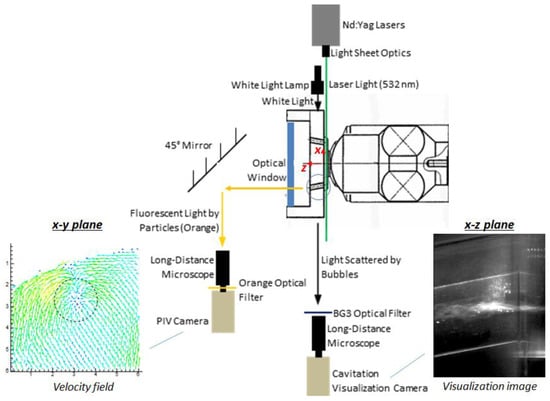
Figure 5.
Optical arrangement for measurements of the flow field in the transverse (x-y) plane normalized to the notional axis of the injector upstream of a nozzle, and flow visualization within the nozzle (x-z plane). Sample results obtained from both techniques are demonstrated.
In order to obtain information for cavitation simultaneously with the flow field (after acquiring the high-speed cavitation images), a second camera (Cavitation visualization camera) with a long-distance microscope was necessary. This camera had a 12-bit conversion with a spatial resolution of 1378 pixels × 1040 pixels, and the long-distance microscope was similar to the one used for PIV measurements. Since a laser was used for the PIV flow velocity measurements, the cavitation images were saturated by the high-power scattered light and by bubbles crossing the laser sheet. For that reason, BG3 optical filters were used (which transmitted only blue light) with a white light lamp in order to provide wavelength separation between the cavitation visualization images and the PIV images, which used the fluorescent light emitted by the particles, and excited by the green light (532 nm) of the Nd: Yag laser. Although this arrangement worked satisfactorily, the lamp, which also emitted light at the fluorescent wavelength, induced some noise into the PIV images. This noise was minimized using neutral density filters optically and through the image processing software, where a median and the maximum filter routines were incorporated to de-noise the images [30]. The use of fluorescent particles was necessary (nominal diameter 1–20 µm, mean diameter 10 µm), which were covered with Rhodamine B dye, in order to separate the fluorescent emission and the elastically scattered light from the cavitation bubble at the laser wavelength, and hence, to distinguish between the gaseous and the liquid phase. The fluorescent light was transmitted through an optical filter, which was placed between the PIV camera and the long-distance microscope.
These results are linked to real injectors since appropriate dimensionless parameters are defined as relating to the flow conditions in the model and to the prototype. This could be achieved using Reynolds and Cavitation Numbers with, as suggested in [31], the Cavitation number being relevant as a dynamic similarity parameter only when the flow cavitated. The Reynolds number is defined as follows:
where Re is the Reynolds number, ρ is the density of the working fluid, Ud is the bulk velocity at a reference section, and d is the characteristic length of the reference section, as illustrated in Figure 1 and Figure 2 (which is taken as the diameter of the needle valve ‘seat’ at the reference section, namely 36 mm for Type A and Type B models, and 50 mm for Type C model) and μ is the dynamic viscosity of the working fluid.
The Cavitation number, formally derived, is as follows:
where σv is the cavitation number, Pd is the static pressure at the reference section, Pv is the vapor pressure of the working fluid at 25 °C (466 Pa), ρ is the density of the working fluid, and Ud is the bulk velocity at the reference section. Note that other expressions for the cavitation number exist in the literature (as presented in [9]), which can replace the dynamic pressure with a pressure drop across the reference point: there are advantages to both definitions. In the present context, we prefer the formal definition above, which relates to changes in dynamic pressure. As seen in [12], the magnitudes of the Cavitation number in our flows were “large” in the sense that, on physical grounds, the Cavitation number compared the liquid static pressure to the dynamic pressure of the flow, and one expected the cavitation to arise when the value of σv was of order unity. This apparent discrepancy arose because of our choice of location for the reference section, which was remote from that of the location of cavitation, and, thus, the resultant values of σv were of the order of thousands. This unusual choice of location for the reference point was made because it was easier to measure the static pressure necessary for the calculation of the Cavitation number. Note that it was formally permissible to define the reference conditions and the location for the cavitation number at any convenient point in the model, provided that we conducted scaling with reference to the same location in the prototype.
The conditions for the visualization of cavitation with a high frame rate camera are shown in Table 1.

Table 1.
Conditions for high frame rate visualization of the gasoline injector models.
The conditions of the PIV measurements and the simultaneous (not at high frame rate) visualization of cavitation were the following: for the Type B model, the Reynolds Number was 11,450, and the Cavitation Number was 2650. For the Type C model, the Reynolds Number was 9200, and the Cavitation Number was 6400.
2.2. Proper Orthogonal Decomposition (POD)
Proper Orthogonal Decomposition, or POD, is a powerful method of data analysis. Based on the Karhunen–Loeve procedure of probability theory [32,33], POD aims at reducing the dimensionality of a dataset while retaining as much as possible the variations present in it [34,35]. The basic idea behind POD is to describe a given statistical ensemble with a minimum number of deterministic modes [36,37].
We considered an ensemble of instantaneous data , with x and t as the spatial and temporal parameters, respectively. In the present work, represents the two-dimensional velocity data from the PIV measurement of liquid velocity just upstream of the nozzles or the image intensity distribution in the shadowgraph images of the nozzles (see Figure 5). The mean velocity or mean intensity is subtracted from the instantaneous values so that the values of represent fluctuations only. For the M number of flow realizations and N number of spatially located data points for each realization, POD decomposes into a sum of the product of spatial eigenvectors and temporal coefficients ; therefore,
where i = 1 to M, j = 1 to N, represents the eigenvalue corresponding to each eigenvector , and r is the rank of the matrix so that . Thus, the POD modes represent the average spatial features of the whole ensemble, while the corresponding coefficients signify their ‘‘weight’’ for the time instants i = 1, 2,…, M, respectively.
The eigenvalues are obtained by solving the eigenvalue equation, , , under the restriction that the norm of is 1, where R is the spatial cross-correlation matrix of size N × N. However, when M << N, as in the present case, the calculation time could be dramatically reduced if the temporal cross-correlation matrix is evaluated instead of ; therefore:
This numerical procedure, as proposed by Sirovich [38], is popularly known as the “method of snapshots”. The solution , leads to the orthonormal temporal coefficients corresponding to the eigenvalues . The symmetry and non-negative definiteness of RT ensures . The eigenvectors are obtained from the inverse relation . The eigenvalues are ordered as , and the corresponding coefficients () and modes () are also arranged accordingly. Hence, the first mode always represents the maximum spatial variations in the liquid velocity fluctuations upstream of the nozzle or the intensity fluctuations in the shadowgraph images of the nozzles. The significant advantage of POD is that due to its fast convergence property, the number of energetically significant modes is minimum. Hence, original intensity data can be reconstructed using only a few modes instead of considering all of them; therefore,
In other words, only a few modes, roptimum (much less than the total number of modes, M), needed to be considered for the data analysis.
The present work used the method of the snapshot described above to obtain the POD modes. For the POD analysis of the PIV data, 1000 instantaneous two-dimensional liquid velocity vector fields (measured upstream of the nozzles) were considered, such that each sample contained a velocity measured at 42 × 42 grid points. In this case, the initial POD modes were considered to be synonymous with the dominant liquid flow structures upstream of the nozzles [39]. For the POD analysis of the shadowgraph images, 1000 instantaneous images were considered. Only certain sections of each shadowgraph image close to the nozzle inlet were considered for the POD calculation in order to optimize the computational time since cavitation was not observed too far downstream of the nozzle. In this case, the initial POD modes depicted the string or edge separation cavitation within the nozzle. The uncertainty in the amplitude of the spatial POD modes was found to be about 10%. However, the uncertainty for eigenvalues, which determined the significance of the modes, was about 1% or even less for all cases.
3. Results
3.1. Visualization of ‘Bulk’ Cavitation
Consecutively acquired cavitation visualization images of the Type A Injector Model are shown in Figure 6. Three of these images (for the instances to, to + 7/4500 s and to + 14/4500 s) are shown in [12]; however, here, the whole series acquired is shown in order for the reader to have a complete understanding of the cavitation evaluation. Note that the flow is from right to left. Two types of cavitation were identified in the flow. The first, which is commonly observed in the literature, is known as edge separation cavitation and is a result of flow separation due to the high associated streamline curvature that occurs at the edge of the nozzle inlet. The second is named ‘bulk’ cavitation and arises far from the walls and, thus, far from the streamline curvature, which is associated with salient points on a wall. The latter could be caused or affected by streamwise vortical structures that are present inside and just upstream of the injection nozzle; however, so far, there is no quantitative experimental flow field evidence for this. Both edge separation cavitation and ‘bulk’ cavitation were present in the flow. Edge separation cavitation is indicated by white dashed circles, and ‘bulk’ cavitation is indicated by white rectangles for the typical visualization images of each case. These were added to the images to assist the reader in identifying the regions that were occupied by ‘bulk’ cavitation or edge separation cavitation compared to the rest of the images. It can be noted that for the Type A model, there is a “scratch” at the surface of the material of the transparent model that is present in all the images of Figure 6, which is indicated by the red rectangle. Figure 6 shows that the edge separation cavitation was present at the bottom edge from to to to + 3/4500 s. From to + 4/4500 s to to + 5/4500 s, cavitation was visible only on the top corner of the nozzle inlet. The “top corner” cavitation could probably be related to the separation region, which is attached to the top corner of the nozzle, as shown in the PIV measurements of the Type A model presented in [25], while there is nothing comparable at the bottom edge. Therefore, the PIV results suggest that cavitation is unexpected at the bottom inlet corner.
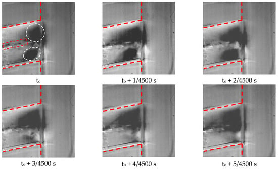
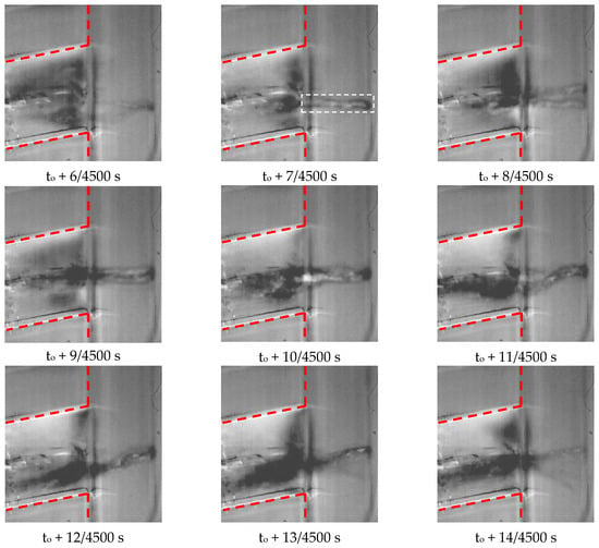
Figure 6.
Cavitation visualization images of the Type A (Nozzle 4) model obtained with high speed camera. Flow is from right to left. White circles indicate edge separation cavitation, and white rectangles indicate string cavitation for typical images. Red rectangle indicates a “scratch” at the model’s surface. Three of these images (for the instances to, to + 7/4500 s and to + 14/4500 s) are shown in [12]. Red dashed lines indicate nozzle boundaries.
At the instant of to + 6/4500 s, the separation cavitation was weaker in comparison to the previous images, and a weak bubble string could be observed. From that moment on, we could see the development and existence of ‘bulk’ cavitation in this nozzle. At time to + 8/4500 s, two strings of the bulk cavitation were visible, but it is unlikely that the second could be cavitation in the nozzle right behind the one of interest because of the small depth of field in the optics. Up to the image at time to + 8/4500 s, the ‘bulk’ cavitation did not seem to extend inside the nozzle. After that time and until to + 11/4500 s, the ‘bulk’ cavitation was also present inside the nozzle, and from that moment until time to + 13/4500 s, the edge separation cavitation and ‘bulk’ cavitation coexisted in the nozzle. In the last image of this series, the two strings seemed to separate and become very thin, so after a few instants, ‘bulk’ cavitation was not present. The presence of the string at first only upstream of the nozzle inlet and then inside the nozzle led us to conclude that it started upstream of the nozzle, which suggested that it was caused by the streamwise vortical structures present at that region which was also the motivation for the PIV measurements appearing normal to the notional axis of the injector, as presented in the next section.
The cavitation visualization images of the Type B model (Figure 7) show that both edge separation and ‘bulk’ cavitation were present again. From the image acquired at time to until the image at time to + 3/4500 s, only edge separation cavitation could be observed, which was located both at the top and bottom corners of the nozzle inlet. In the picture, at time to + 4/4500 s, a weak string appeared, and from that moment on until time to + 8/4500 s, a clear string was present in the examined nozzle. From time to + 9/4500 s, the image of the string became very weak, and then only edge separation cavitation was present at both inlet corners. Therefore, edge separation cavitation was present during the time that ‘bulk’ cavitation occurred.
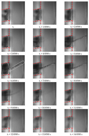
Figure 7.
Cavitation visualization images of Type B (Nozzle 4) model obtained with high speed camera. White circles indicate edge separation cavitation and white rectangles represent string cavitation for typical images. Flow is from right to left. Red dashed lines indicate nozzle boundaries.
It is noted that the Type B model had a larger nozzle plenum just upstream of the nozzle in comparison to the Type A model, as can be concluded by the geometry of the injector models presented in the earlier text. Although from purely geometrical considerations, rstreamline, where rstreamline is the radius of the curvature for the streamlines that enter the nozzle, might be different between the two models and it was hard to draw any conclusions since the static pressure field was related to ρU2/rstreamline. The presence of ‘bulk’ cavitation appeared to affect the existence of edge separation cavitation, at least at the initial development stages of the string, since at the initial development stages of the string for the Type A model, edge separation cavitation was not present. When a string appeared, the liquid that entered the nozzle met an abrupt turn in the flow direction near the inlet corner of the Type A model, restricted edge separation, and, as a consequence, the edge separation cavitation was not present. During these stages, it might be that the liquid flow at the region where edge separation usually happens was settling without forming a recirculation, which could reduce the local pressure below the boiling point (466 Pa as explained in [40]) since the flow around that section was occupied by the string. In the case of the Type B model, the streamline curvature as the liquid entered the nozzle might be smaller than Type A; therefore, smaller recirculation zones were formed at the inlet edges, which were not disrupted by the presence of the strings. This could be the reason why, for the type B model, ‘bulk’ cavitation and edge separation cavitation coexisted at all times. This might be a useful conclusion for the design of the injector. Although we refer to gasoline injectors here, this could also be applicable to diesel and other types of injectors.
The cavitation visualization images of the Type C Injector are illustrated in Figure 8. Again, three of these images (for the instances to, to + 7/4500 s and to + 14/4500 s) are shown in [12], and for the same reason, as Type A is also presented here. In this case, three main conclusions can be drawn. First, in all the images, there was a continuous presence of ‘bulk’ cavitation, with the string “precessing”, which at least suggested that the lifetime of ‘bulk’ cavitation was longer in this case than in the other types. Secondly, the diameter of the string in these images was significantly larger than for Type A and Type B models; therefore, it could be said that, in this case, whatever the flow structure that gave rise to cavitation and was a result of the geometry of the injector, this allowed the longer presence of cavitation. Thirdly, bubbles seemed to cover the whole nozzle region since this was all shadowed, although it was not possible to decide from the images if this was also a result of edge separation cavitation.
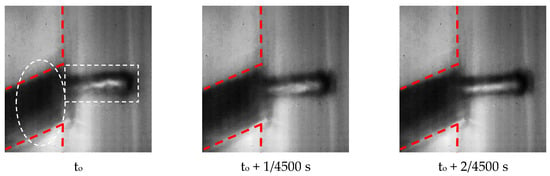
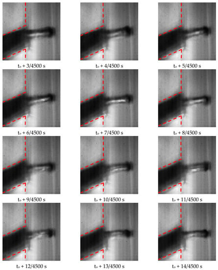
Figure 8.
Cavitation visualization images of the Type C model (Nozzle 5) obtained with high-speed camera. Flow is from right to left. White circles indicate edge separation cavitation, and white rectangles indicate string cavitation for typical images. Three of these images (for the instances to, to + 7/4500 s and to + 14/4500 s) are shown in [12]. Red dashed lines indicate nozzle boundaries.
3.2. Mean Flow Field and Cavitation Visualization
Velocity measurements at the planes just upstream of the nozzles were conducted, and the results are illustrated for the cases where ‘bulk’ cavitation was present. More specifically, for the Type B injector model, the results are illustrated for nozzle 1 and nozzle 4 (present at the edge and the interior locations, respectively, as shown in Figure 1). Simultaneously with the fluorescent PIV liquid velocity measurements, the cavitation was visualized in order to see if ‘bulk’ cavitation was present or not. The PIV results were averaged over 1000 images, and the cavitation visualization images were typical shadowgraph images. For nozzle 1 (Figure 9), only corner-separation cavitation was present, and the average, at least for the flow field just upstream of the nozzle, had only a weak clockwise swirling motion. In the case of nozzle 4 (Figure 10), where ‘bulk’ cavitation was present, the mean flow field just upstream had no mean swirl but was similar to a “potential flow sink with cross flow” (specifically, the internal flow inside the half body solution).
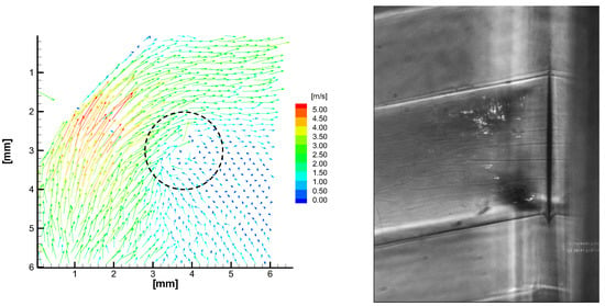
Figure 9.
Left hand side (LHS): time-averaged liquid velocity measurements in the “plane of measurement”, just upstream of the entrance to nozzle 1 (please refer to Figure 5) for Type B model. Right-hand side (RHS): visualization of cavitation (image plane is parallel to that of Figure 1). The dashed circle refers to the nozzle location.
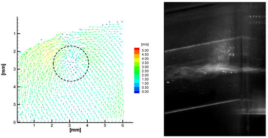
Figure 10.
Left hand side (LHS): time-averaged liquid velocity measurements in the “plane of measurement”, just upstream of the entrance to nozzle 4 (please refer to Figure 5) for Type B model. Right-hand side (RHS): visualization of cavitation (image plane is parallel to that of Figure 1). The dashed circle refers to the nozzle location.
These results are surprising for two reasons. First, we would reasonably expect ‘bulk’ cavitation to be associated with the swirling flow centered on the nozzle; however, this did not seem to be the case. Secondly, we might reasonably expect the swirling flow to inhibit edge cavitation; however, this was also not the case. Quite why the initiation of ‘bulk’ cavitation was promoted by this sink-like flow is not clear. One possible explanation is that the flow measurements were time-averaged values and not representative of the instantaneous flow, which could give rise to cavitation at specific times in the flow.
Flow velocity measurements were also conducted for the Type C model (see Figure 2). Referring to the same figure, we considered nozzle 1, nozzle 6 (which are located at the edge), and nozzle 5 (interior nozzle) to demonstrate different cavitation types. Figure 11, Figure 12 and Figure 13 presents the mean velocity field and cavitation visualization images for different nozzles of the Type C injector. It was observed that for nozzle 5 (Figure 12), which showed ‘bulk’ cavitation, an approximately sink-like flow was present. For nozzles 1 and 6 (Figure 11 and Figure 13, respectively), edge separation cavitation was present, and the flow formed two vortices just upstream of the nozzle inlet, which was different for the sink-like flow that was observed just upstream of nozzle 5. It is very important for the designer that, in both injector models, the flow field just upstream of nozzles shows a ‘bulk’ cavitation that is qualitatively similar since the designer can induce geometry features that promote or inhibit this kind of flow.
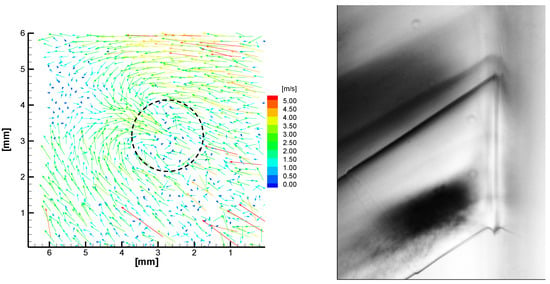
Figure 11.
Left hand side (LHS): time-averaged liquid velocity measurements in the “plane of measurement”, as defined in Figure 2, just upstream of the entrance to nozzle 1 (please refer to Figure 5) for Type C model. Right-hand side: visualization of cavitation (image plane is parallel to that of Figure 2). The dashed circle refers to the nozzle location.
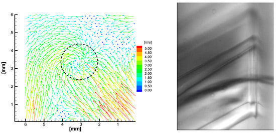
Figure 12.
Left hand side (LHS): time-averaged liquid velocity measurements in the “plane of measurement”, as defined in Figure 2, just upstream of the entrance to the nozzle 5 (please refer to Figure 5) for Type C model. Right-hand side: visualization of cavitation (image plane is parallel to that of Figure 2). The dashed circle refers to the nozzle location.
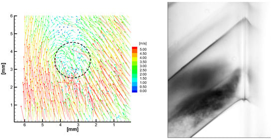
Figure 13.
Left hand side (LHS): time-averaged liquid velocity measurements in the “plane of measurement”, as defined in Figure 2, just upstream of the entrance to the nozzle 6 (please refer to Figure 5) for Type C model. Right-hand side: visualization of cavitation (image plane is parallel to that of Figure 2). The dashed circle refers to the nozzle location.
Obtaining PIV measurements simultaneously with cavitation visualization images at nozzles 1, 5, and 6 (refer to Figure 5 as mentioned above) was conducted because the remaining nozzles were positioned symmetrically with respect to the examined ones and were expected to show the same results. This is the reason why the flows in the three nozzles were examined for the Type C model and in two nozzles for Type B (with Type A needle valve).
3.3. Proper Orthogonal Decomposition (POD) of Liquid Velocity Field in Cavitating Flow Conditions
POD was applied to the instantaneous liquid velocity fields just upstream of the nozzles to captivate the flow conditions, as shown in the previous section. The sum of all the eigenvalues represents the total turbulent kinetic energy of the flow since the decomposition occurred over the fluctuations of the liquid velocity from the mean value. The distribution of the eigenvalues for the nozzle Type B injector model with respect to the mode number is shown in Figure 14. These decreased rapidly after about the first 10 initial modes. Therefore, the eigenvectors corresponding to the first few eigenvalues were expected to correspond to the dominant turbulent structures of the liquid flow.
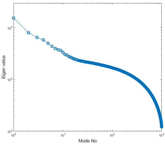
Figure 14.
Eigenvalue spectrum for the fluctuating velocity components u and v for the Type B injector model.
The first two POD modes are presented in Figure 15 and in Figure 16. We can observe that the very first mode (Figure 15) depicted the presence of a vortical structure. The first mode had the maximum average correlation with all the instantaneous velocity fields, and hence, it represents the most common flow structure. Thus, in the present case, it could be correlated with the presence of ‘bulk’ cavitation since the flow conditions were selected so that ‘bulk’ cavitation was present. It is worth noting that this vortical structure was not present in the mean flow field results. The second mode (Figure 16) was qualitatively different and not obviously related to a flow structure that could promote ‘bulk’ cavitation.
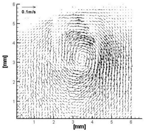
Figure 15.
POD Mode 1 of the liquid velocity field for the Type B injector model.
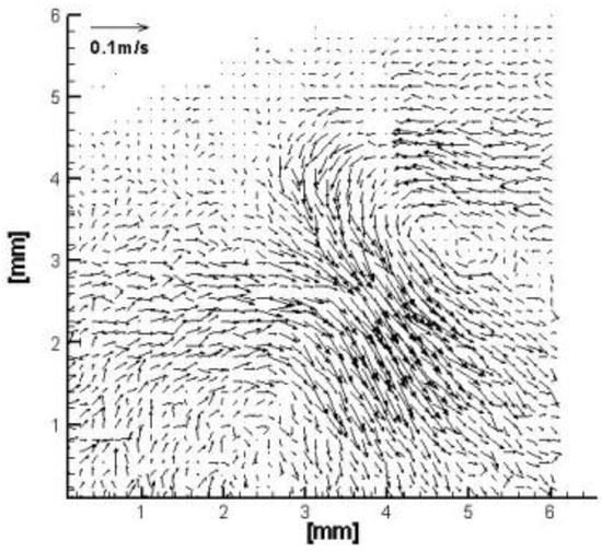
Figure 16.
POD Mode 2 of the liquid velocity field for the Type B injector model.
In order to estimate if the pressure drop in relation to this vortical structure could lead to ‘bulk’ cavitation, the instantaneous velocity field of Type B was reconstructed by considering the first mode only. Figure 17 below shows a typical radial profile of absolute velocity, where point ‘0′ corresponds to the position of the nozzle center. The POD mode 1 signifies the existence of a free vortex or, strictly speaking, a Rankine vortex since the fluid possesses finite viscosity. Therefore, away from the nozzle axis, the tangential velocity first increased and then decreased close to the outer wall. At the radius of the order of the nozzle radius (2 mm), the tangential fluid velocity was about 1 m/s. Since the angular momentum of the vortical structure had to be conserved, the tangential velocity was inversely proportional to the radius or Hence, when the vortical structure entered the nozzle, the fluid velocity increased close to its axis. Therefore, at and , the fluid velocity accelerated to about 10 m/s and 20 m/s, respectively. Assuming that far away from the axis of the vortex, the pressure was atmospheric, and the tangential velocity was zero, represent the minimum pressure drop necessary to initiate cavitation. The actual pressure drop was , and therefore, the ratio was found to be equal to about 2 and 0.5 for and . This means ‘bulk’ cavitation must occur close to the nozzle axis. Since both pressure drop and vorticity proportionally increase with the inverse of the square from the distance from the nozzle, a small initial rotation of the fluid upstream of the nozzle is sufficient to create a concentrated vortex inside the nozzle, which can cavitate the liquid. It should be noted that this is the first time that proof has been provided that the local flow characteristics can cause cavitation. In previous studies, the emphasis has been on the gas entrained inside the nozzle from the environment outside the nozzle or by gas phase components that remain in the injector sac volume by previous injection events. Due to the experimental arrangement of the current study, the previously proposed mechanisms of explaining cavitation in the literature, according to the previous sentence, cannot occur. In this way, only specific instantaneous flow structures can induce cavitation.
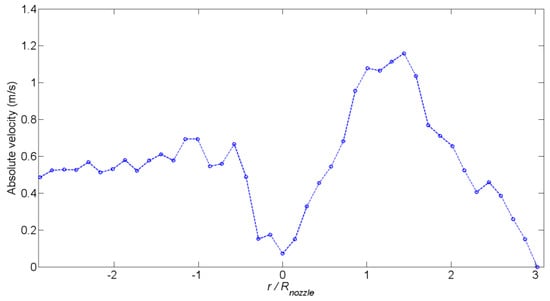
Figure 17.
Typical reconstructed radial profile of the absolute velocity of the Type B injector model using POD mode 1 at the plane of the measurement just upstream of Nozzle 4 (see Figure 1). Point ‘0′ corresponds to the position of the nozzle axis.
The eigenvalue spectrum for the corresponding nozzle of the Type C injector model is shown in Figure 18. The trend of the eigenvalue spectrum for the fluctuating liquid velocity components was similar to the corresponding nozzle of the Type B model, with a sharp decrease in the initial eigenvalues. Again, this means that the dominant liquid flow structures are represented by the first few modes. The first mode for this case is illustrated in Figure 19, which again shows a vortical structure, which might be responsible for the formation of ‘bulk’ cavitation. Higher modes are associated with flow structures that have smaller length scales.
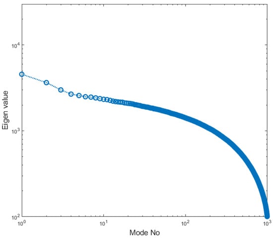
Figure 18.
Eigenvalue spectrum for the fluctuating liquid velocity components u and v for the Type C injector model.
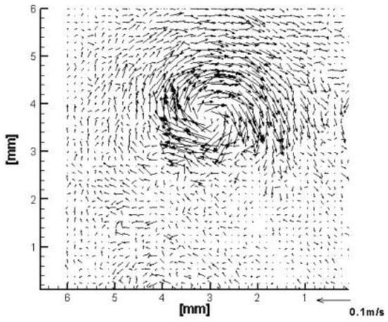
Figure 19.
POD Mode 1 of the liquid velocity field for the Type C injector model.
3.4. POD of Shadowgraphic Cavitation Images of Type B Injector Model
POD was applied to the intensity of the shadow graphic cavitation images (those acquired simultaneously with PIV, so 1000 images for each nozzle) for nozzle 1 and nozzle 4 (see Figure 1) of the Type B injector model. This technique was not applied to the Type C model because the multiple nozzles were densely located, and there was noise generated on the shadow graphic images by the presence of cavitation in the nozzles located behind nozzles 1, 5, and 6 (Figure 2) for which PIV data have been acquired and examined. Figure 20 shows the first two modes of POD’s application to the shadow graphic cavitation images for the Type B injector model.
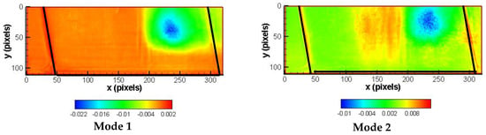
Figure 20.
POD modes 1 and 2 for the shadow graphic cavitation images of Nozzle 4 (see Figure 1) of the Type B injector model. Flow is upwards (different orientation from that of Figure 1). The color of the contour plots refers to the fluctuations in pixel intensity values for the shadow graphic images. Nozzle borders are marked with black lines.
It should be noted that the liquid flow in the images of Figure 20 has an upward direction. The original shadow graphic images were contaminated due to unwanted reflected light. Therefore, modes 1 and 2 show a bright spot (blue color in the contour plots of Figure 20) near the right edge of the nozzle, which does not correspond to edge separation cavitation, but the intensity of reflected light. To avoid these effects, POD was applied to the original images after cropping the right side, and the first four POD modes are shown in Figure 21.
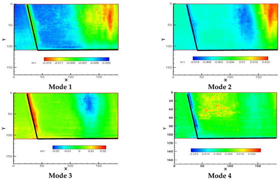
Figure 21.
POD modes 1, 2, 3 and 4 of the shadow graphic cavitation images for Nozzle 4 (see Figure 1) of the Type B injector model after cropping the right-hand side of the original shadow graphic images. Flow is upwards (different orientation than that of Figure 1). The color of the contour plots refers to the fluctuations in pixel intensity values for the shadow graphic images. Nozzle borders are marked with black lines.
The first three modes of Figure 21 clearly depict the presence of ‘bulk’ cavitation. It should be noted that the right-hand side of Figure 21 corresponds nearly to the axis of the nozzle flow, as the reader can notice by comparing the coordinates between the images of Figure 20 and Figure 21. Edge separation cavitation appeared for mode 4. In addition, the first four POD modes of the shadowgraphs in nozzle 1 (see Figure 1) are the same as the injector model presented in Figure 22.
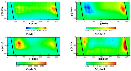
Figure 22.
POD modes 1, 2, 3 and 4 of the shadow graphic cavitation images of Nozzle 1 (see Figure 1) of the Type B injector model. Flow is upwards (different orientation than that of Figure 1). The color of the contour plots refers to the fluctuations in pixel intensity values of the shadow graphic images. Nozzle borders are marked with black lines.
Figure 22 shows that edge-separation cavitation was present for all the modes shown. If we examine the eigenvalue contribution of each mode (Figure 23), we can observe that for nozzle 4 (see Figure 1), the contribution of the first three modes where ‘bulk’ cavitation was observed was approximately 45% of the total value, while, for nozzle 1 (see Figure 1), the contribution of the first four modes, where we only had edge separation cavitation, was 80% of the total value. These percentages represent the probabilities of having a ‘bulk’ or edge separation cavitation in the flow of the examined nozzles. Therefore, in nozzle 4 (see Figure 1) of the Type B injector model, the probability of having ‘bulk’ cavitation was about 45%, while, in nozzle 1 of the same model, the probability of having edge separation cavitation was about 80%. So, the probability of having ‘bulk’ cavitation in nozzle 1 was low, which could be verified by observing the shadow graphic cavitation images of nozzle 1, ‘bulk’ cavitation was not present at all.
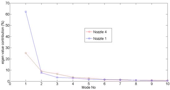
Figure 23.
Eigenvalue contribution of each of the first 10 modes of the shadow graphic cavitation images of Nozzles 1 and 4 in Figure 1 of the Type B injector model.
4. Conclusions
In this work, ‘bulk’ cavitation was studied in three gasoline multi-hole injectors. Two-dimensional micron resolution Particle Imaging Velocimetry was employed to measure the internal flow field of the 10:1 super-scale transparent models of multi-hole injectors just upstream of the entrance to the holes of the injector plates in the vicinity of an operating regime just after the onset of cavitation. Our motivation was to understand the physics behind the formation of bulk cavitation and its correlation with the injector flow field. ‘Bulk’ cavitation was found to be present in the specific nozzles of three geometrically different injector models by means of fast camera visualization, where the time evolution of cavitation was also recorded. For Type A and Type B injector models, ‘bulk’ cavitation was not always present, while for the case of the Type C injector model, ‘bulk’ cavitation was present for all the images of cavitation visualization, which indicated that the residence time of ‘bulk’ cavitation in this type of injector was longer compared to the other injector models.
The liquid flow field at the nozzles of the two injector models (Type B and Type C) was quantified, and it was found that the mean liquid flow velocity just upstream of the exit holes resembled, as expected, the internal flow inside the half body corresponding to the classical potential flow solution for a sink with cross flow. We expected, a priori, ‘bulk’ cavitation to be associated with the existence of the swirling flow centered on the nozzle axis at a given instant. However, we found no such swirling flow structure in the mean flow field results. We thus applied Proper Orthogonal Decomposition (POD) to the instantaneous velocity data in order to identify the dominant liquid flow structures, which could be related to cavitation. It was found that “mode 1” eigenvalues indeed corresponded to swirling flow structures and were dominant for the cases when ‘bulk’ cavitation was present for both injector models where the flow was quantified. This might be related to the origin of ‘bulk’ cavitation. It is the first time that quantitative flow field experimental evidence has been presented, identifying that the above local flow structures could be related to local ‘bulk’ cavitation.
Finally, we applied POD to the shadow graphic cavitation images of the Type B injector model, and the eigenvalue contribution of each mode depicting ‘bulk’ cavitation was found to be representative of the probability of having this kind of cavitation.
In summary, this paper has demonstrated for the first time in a quantitative way the importance of instantaneous liquid flow structures on the initiation of different types of cavitation in injector nozzles. It highlights the importance of describing the instantaneous flow structures in computations of such flows in order to predict the different types of cavitation that can occur and the associated probability of their appearance and time-dependent behavior.
Author Contributions
Conceptualization, Y.H., A.M.K.P.T. and A.A.; methodology, D.K. and S.S.; software, D.K. and S.S.; validation, D.K. and S.S.; formal analysis, D.K. and S.S.; investigation, D.K. and S.S.; resources, Y.H., A.M.K.P.T. and A.A.; data curation, D.K. and S.S.; writing—original draft preparation, D.K. and S.S.; writing—review and editing, Y.H. and A.T; visualization, D.K.; supervision, Y.H. and A.T; project administration, Y.H. and A.T; funding acquisition, Y.H., A.T. and A.A. All authors have read and agreed to the published version of the manuscript.
Funding
This research was funded by Keihin Corporation, Japan.
Data Availability Statement
The data presented in this study are available on request from the corresponding author.
Acknowledgments
We acknowledge Keihin Corporation Japan for providing financial support and the optical injector models.
Conflicts of Interest
The authors declare no conflict of interest.
References
- Payri, F.; Bermudez, V.; Payri, R.; Salvador, F.J. The influence of cavitation on the internal flow and the spray characteristics in diesel injection nozzles. Fuel 2004, 83, 419. [Google Scholar] [CrossRef]
- Ulrich, H.; Lehnert, B.; Guénot, D.; Svendsen, K.; Lundh, O.; Wensing, M.; Berrocal, E.; Zigan, L. Effects of liquid properties on atomization and spray characteristics studied by planar two-photon fluorescence. Phys. Fluids 2022, 34, 083305. [Google Scholar] [CrossRef]
- Oda, T.; Hiratsuka, M.; Goda, Y.; Kanaike, S.; Ohsawa, K. Experimental and Numerical Investigation about Internal Cavitating Flow and Primary Atomization of a Large-Scaled VCO Diesel Injector with Eccentric Needle; ILASS-Europe: Brno, Czech Republic, 2010. [Google Scholar]
- Watanabe, H.; Nishikori, M.; Hayashi, T.; Suzuki, M.; Kakehashi, N.; Ikemoto, M. Visualization analysis of relationship between vortex flow and cavitation behaviour in diesel nozzle. Int. J. Engine Res. 2015, 16, 5. [Google Scholar] [CrossRef]
- Zhong, W.; He, Z.; Wang, Q.; Shao, Z.; Tao, X. Experimental study of flow regime characteristics in diesel multi-hole nozzles with different structures and enlarged scales. Int. Commun. Heat Mass Transf. 2014, 59, 1. [Google Scholar] [CrossRef]
- McGinn, P.; Tretola, G.; Vogiatzaki, K. Unified modeling of cavitating sprays using a three-component volume of fluid method accounting for phase change and phase miscibility. Phys. Fluids 2022, 34, 082108. [Google Scholar] [CrossRef]
- Kim, J.H.; Nishida, K.; Yoshizaki, T.; Hiroyasu, H.H. Characterization of Flows in the Sac Chamber and the Discharge Hole of a D.I. Diesel Injection Nozzle by Using a Transparent Model Nozzle. SAE Tech. Pap. 1997, 972942, 11–23. [Google Scholar]
- Arcoumanis, C.; Flora, H.; Gavaises, M.; Badami, M.M. Cavitation in Real–Size Multi–Hole Diesel Injector Nozzles; SAE International: Diego County, CA, USA, 2000; Volume 109, pp. 1485–1500. [Google Scholar]
- Arcoumanis, C.; Flora, H.; Gavaises, M.; Kampanis, N.; Horrocks, R. Investigation of Cavitation in a Vertical Multi-Hole Injector; SAE International: Diego County, CA, USA, 1999; Volume 108, pp. 661–678. [Google Scholar]
- Gilles-Birth, I.; Bernhardt, S.; Spicher, U.; Rechs, M. A Study of the In-Nozzle Flow Characteristics of Valve Covered Orifice Nozzles for Gasoline Direct Injection. SAE Tech. Pap. 2005, 1, 3684. [Google Scholar]
- Nouri, J.M.; Mitroglou, N.; Yan, Y.; Arcoumanis, C. Internal Flow and Cavitation in a Multi-hole Injector for Gasoline Direct-Injection Engines. SAE Tech. Pap. 2007, 1, 1405. [Google Scholar]
- Kolokotronis, D.; Hardalupas, Y.; Taylor, A.M.K.P.; Aleiferis, P.G.; Arioka, A.; Saito, M. Experimental Investigation of Cavitation in Gasoline Injectors. SAE Tech. Pap. 2010, 1, 1500. [Google Scholar]
- Reid, B.A.; Hargrave, G.K.; Garner, C.P.; Wigley, G. An investigation of string cavitation in a true-scale fuel injector flow geometry at high pressure. Phys. Fluids 2010, 22, 031703. [Google Scholar] [CrossRef]
- Mitroglou, N.; McLorn, M.; Gavaises, M.; Soteriou, C.; Winterbourne, M. Instantaneous and ensemble average cavitation structures in Diesel micro-channel flow orifices. Fuel 2014, 116, 736. [Google Scholar] [CrossRef]
- Reid, B.A.; Gavaises, M.; Mitroglou, N.; Hargrave, G.K.; Garner, C.P.; Long, E.J.; McDavid, R.M. On the formation of string cavitation inside fuel injectors. Exp. Fluids 2014, 55, 1662. [Google Scholar] [CrossRef]
- Giannadakis, E.; Gavaises, M.; Arcoumanis, C. Modelling of cavitation in diesel injector nozzles. J. Fluid Mech. 2008, 616, 153. [Google Scholar] [CrossRef]
- Gavaises, A.M.; Arcoumanis, C.C. Vortex flow and cavitation in diesel injector nozzles. J. Fluid Mech. 2008, 610, 195. [Google Scholar]
- Gavaises, M.; Andriotis, A.; Papoulias, D.; Mitroglou, N.; Theodorakakos, A. Characterization of string cavitation in large-scale Diesel nozzles with tapered holes. Phys. Fluids 2009, 21, 52. [Google Scholar] [CrossRef]
- Salvador, F.J.; Romero, J.V.; Rosello, M.D.; Martinez-Lopez, J. Validation of a code for modelling cavitation phenomena in Diesel injector nozzles. Math. Comput. Model. 2010, 52, 1123. [Google Scholar] [CrossRef]
- Chang, N.A.; Yakushiji, R.; Dowling, D.R.; Ceccio, S.L. Cavitation visualization of vorticity bridging during the merger of co-rotating line vortices. Phys. Fluids 2007, 19, 058106. [Google Scholar] [CrossRef]
- Choi, J.; Ceccio, S.L. Dynamics and noise emission of vortex cavitation bubbles. J. Fluid Mech. 2007, 575, 1. [Google Scholar] [CrossRef]
- Walther, J.; Schaller, J.K.; Wirth, R.; Tropea, C. Characterization of Cavitating Flow Fields in Transparent Diesel Injection Nozzles Using Fluorescent Particle Image Velocimetry (FPIV). In Proceedings of the ILASS 2000, Darmstadt, Germany, 11–13 September 2000. [Google Scholar]
- Roth, M.H.; Gavaises, M.; Arcoumanis, C. Cavitation Initiation, Its Development and Link with Flow Turbulence in Diesel Injector Nozzles; SAE International: Diego County, CA, USA, 1999; Volume 111, pp. 561–580. [Google Scholar]
- Allen, J.; Hargrave, G.; Khoo, Y. In-Nozzle and Spray Diagnostic Techniques for Real-Sized Pressure Swirl and Plain Orifice Gasoline Direct Injectors. SAE Tech. Pap. 2003, 1, 3151. [Google Scholar]
- Aleiferis, P.G.; Hardalupas, Y.; Kolokotronis, D.; Taylor, A.M.K.P.; Arioka, A.; Saito, M. Experimental Investigation of the Internal Flow Field of a Model Gasoline Injector Using Micro-Particle Image Velocimetry. SAE Trans. J. Fuels Lubr. 2006, 115, 597. [Google Scholar]
- Aleiferis, P.G.; Hardalupas, Y.; Kolokotronis, D.; Taylor, A.M.K.P.; Kimura, T. Investigation of the Internal Flow Field of a Diesel Model Injector Using Particle Image Velocimetry and CFD. SAE Tech. Pap. 2007, 1, 1897. [Google Scholar]
- Mauger, C.; Méès, L.; Michard, M.; Azouzi, A.; Valette, S. Shadowgraph, Schlieren and interferometry in a 2D cavitating channel flow. Exp. Fluids 2012, 53, 1895. [Google Scholar] [CrossRef]
- Mauger, C.; Méès, L.; Michard, M.; Lance, M. Velocity measurements based on shadowgraph-like image correlations in a cavitating micro-channel flow. Int. J. Multiph. Flow 2014, 58, 301. [Google Scholar] [CrossRef]
- Mauger, C. Cavitation in a Diesel Injector Model Micro-Channel: Visualization Methods and Influence of Surface Condition. Ph.D. Thesis, École Centrale Lyon, Lyon, France, 2012. [Google Scholar]
- Charalambides, G. Charge Stratified HCCI Engine. Ph.D. Thesis, Department of Mechanical Engineering, Imperial College London, London, UK, 2006. [Google Scholar]
- Franc, J.P.; Michel, J.M. Fundamentals of Cavitation; Kluwer Academic Publishers: Dordrecht, The Netherlands, 2004; ISBN 1-4020-2232-8. [Google Scholar]
- Loeve, M.M. Probability Theory; van Nostrand: Princeton, NJ, USA, 1955. [Google Scholar]
- Golub, G.; Loan, C.V. Matrix Computations; North Oxford Academic: Oxford, UK, 1983. [Google Scholar]
- Kumar, A.; Sahu, S. Liquid jet disintegration memory effect on downstream spray fluctuations in a coaxial twin-fluid injector. Phys. Fluids 2020, 32, 073302. [Google Scholar] [CrossRef]
- Charalampous, G.; Hadjiyiannis, C.; Hardalupas, Y. Proper orthogonal decomposition of primary breakup and spray in co-axial airblast atomizers. Phys. Fluids 2019, 31, 043304. [Google Scholar] [CrossRef]
- Charalampous, G.; Hardalupas, Y. Application of Proper Orthogonal Decomposition to the morphological analysis of confined co-axial jets of immiscible liquids with comparable densities. Phys. Fluids 2014, 26, 113301. [Google Scholar] [CrossRef]
- Kumar, A.; Sahu, S. Large scale instabilities in coaxial air-water jets with annular air swirl. Phys. Fluids 2019, 31, 124103. [Google Scholar] [CrossRef]
- Sirovich, L. Turbulence and the dynamics of coherent structures. Q. Appl. Math. 1987, 45, 561–571. [Google Scholar] [CrossRef]
- Lumley, J.L. The structure of inhomogeneous turbulent flows. In Proceedings of the International Colloqium on the Fine Scale Structure of the Atmosphere and its Influence on Radio Wave Propagation, Nauka, Moscow, 1967. [Google Scholar]
- Kolokotronis, D. Experimental Investigation of the Internal Flow Field of Model Fuel Injectors. Ph.D. Thesis, Department of Mechanical Engineering, Imperial College London, London, UK, 2007. [Google Scholar]


Disclaimer/Publisher’s Note: The statements, opinions and data contained in all publications are solely those of the individual author(s) and contributor(s) and not of MDPI and/or the editor(s). MDPI and/or the editor(s) disclaim responsibility for any injury to people or property resulting from any ideas, methods, instructions or products referred to in the content. |
© 2023 by the authors. Licensee MDPI, Basel, Switzerland. This article is an open access article distributed under the terms and conditions of the Creative Commons Attribution (CC BY) license (https://creativecommons.org/licenses/by/4.0/).