Frequency and Amplitude Modulations of a Moving Structure in Unsteady Non-Homogeneous Density Fluid Flow

Abstract

A fluid-structure interaction’s effects on the dynamics of a hydrofoil immersed in a fluid flow of non-homogeneous density is presented and analyzed. A linearized model is applied to solve the fluid-structure coupled problem. Fluid density variations along the hydrofoil upper surface, based on the sinusoidal cavity oscillations, are used. It is shown that for the steady cavity case, the value of cavity length $L_p$ does not affect the amplitude of the hydrofoil displacements. However, the natural frequency of the structure increases according to $L_p$. In the unsteady cavity case, the variations of the added mass and added damping (induced by the fluid density rate of change) generate frequency and amplitude modulations in the hydrofoil dynamics. To analyse this phenomena, the empirical mode decomposition, a well established data-driven method to handle such modulations, is used.

1. Introduction

Fluid structure interaction (FSI) problems occur when the fluid loading greatly affects the structure’s dynamics and the structure displacement locally affects the fluid flow. Initially studied with simplified models, the simulation of complex coupled problems has developed considerably in recent years. The state-of-the-art in this field is now very mature and several papers with different fields of application domains can be found in the literature [1,2,3].

The new challenge of FSI problem analysis consists in taking into account complex phenomena, observed both in fluid and solid mechanics, especially in the field of fluids where the dynamics are subjected to many physical quantities such as velocity, pressure, density or temperature. This work focuses on FSI effects in a non-homogeneous density flow. Recent work has pointed out that two-phase flow has an impact on the fluid structure interaction for various devices, such as propeller blades or hydrofoils [4,5,6,7,8,9]. However, very few published works address the problem of estimating this impact on the structure dynamics. This work is strongly motivated by recent advances in experimental and modeling studies carried out by the authors. It is shown that modal response of the structure could be modified in the presence of cavitation [10]. This modification can be attributed to the presence in the flow of a non stationary liquid-vapor mixture with a strong variation in density at the fluid structure interface. Previous works proposed the decomposition of the fluid variables into two components: the first component is related to the fluid flow around the non-vibrating structure while the second one describes the fluid flow induced by the structure vibrations [11]. This approach can be used to compute the added mass and the added damping operators for complex geometries and complex fluid flow behaviour. Here, the fluid flow is characterized by oscillating cavity on the fluid-structure interface. Unlike to homogeneous fluid case, it is shown that the added mass operator is not symmetrical and depends on the flow through fluid density variations at the fluid-structure interface. Also, it was shown that variation rate of the fluid density induces an added damping operator. This suggests a possible variation of the natural frequency of the structure related to the variation of added mass. It is reported in [11] that the fluid density variations on the fluid-structure interface have an effect on the added mass operator and the variation rate of this density induces an added damping operator.

The aim of this paper is to study the effect of these variations on the structure dynamics. First, the modeling of the structure dynamics is carried out. A rigid section of a hydrofoil immersed in a 2D fluid flow and supported by a linear spring, is considered. Equations of the hydrofoil motion are thus provided. Second, a model of the fluid flow generated by the displacements of the structure is considered to determine the hydrodynamic loads. This is given by the solution of a Laplace equation, with the space variations of the fluid density taken into account. Applied to the structure dynamics, the hydrodynamic loads act as an added mass and an added damping. A simplified model of an unsteady cavity, based on a sheet cavitation oscillation, is used to take into account the time and space variations of the fluid density on the fluid-structure interface. The empirical mode decomposition (EMD) [12] is used to analyze the structure displacement. The displacement signal is decomposed by EMD into intrinsic mode functions (IMFs), followed by the instantaneous frequencies estimation of these sifted IMFs that evidence the frequencies modulations.

2. Fluid Loads Acting on the Immersed Structure

A 2D rigid section of hydrofoil type NACA0012 (${\Omega }_S$), immersed in a 2D fluid flow (${\Omega }_F$) and animated by a heave motion, is considered (Figure 1). The fluid domain boundaries are respectively the flow inlet ${\Gamma }_I$, the flow outlet ${\Gamma }_O$, the fixed boundary (wall) ${\Gamma }_W$ and the fluid-structure interface (moving boundary) ${\Gamma }_{FS}={\Omega }_F\cap {\Omega }_S$. $\mathbf{n}$ denotes the outward normal unit vector at $\partial {\Omega }_F={\Gamma }_I\cup {\Gamma }_O\cup {\Gamma }_W\cup {\Gamma }_{FS}$. $\overrightarrow{U_{\infty }}$ is the uniform velocity field of the fluid upstream of the hydrofoil. Parameter $\theta$ corresponds to the angle of incidence of the hydrofoil.

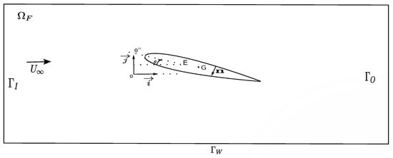
Figure 1. Fluid and Structure domains.

In this study, a non-homogeneous inviscid fluid flow is considered. The corresponding conservation equations are given by:

$$\left\{\begin{array}{cccc}\hfill \frac{\partial \rho }{\partial t}+\nabla ·\left(\rho u\right)& =0\hfill & \mathrm{on} {\Omega }_F\hfill & \hfill \left(a\right)\\ \hfill \frac{\partial \left(\rho u\right)}{\partial t}+\nabla ·(\rho u\otimes u)& =-\nabla p\hfill & \mathrm{on} {\Gamma }_{FS}\hfill & \hfill \left(b\right)\end{array}\right.$$

(1)

where u, p and $\rho$ are respectively the time and space-dependent fluid velocity, fluid pressure and two-phase fluid density. Density $\rho$ can change from liquid, ${\rho }_L$, to vapor ${\rho }_V$ (or vice versa). The boundary conditions are given by:

$$\left\{\begin{array}{cccc}\hfill u& =u_{\infty }\hfill & \mathrm{on} {\Gamma }_I\hfill & \hfill \left(c\right)\\ \hfill -p\mathbf{n}& =0\hfill & \mathrm{on} {\Gamma }_O\hfill & \hfill \left(d\right)\\ \hfill u·\mathbf{n}& =0\hfill & \mathrm{on} {\Gamma }_W\hfill & \hfill \left(e\right)\\ \hfill u·\mathbf{n}& ={\dot{\xi }}_y{n}_y\hfill & \mathrm{on} {\Gamma }_{FS}\hfill & \hfill \left(f\right)\end{array}\right.$$

(2)

where $n_y$ and ${\dot{\xi }}_y$ are respectively the $\mathbf{j}$ components of the normal unit vector $\mathbf{n}$ and the velocity $\dot{\xi }$ of a point A(x,y) on the interface ${\Gamma }_{FS}$ given by Equation (12).

Let us assume the following decomposition:

$$u=\tilde{u}+u^{\prime },\mathrm{and}p=\tilde{p}+p^{\prime }$$

(3)

Assuming that $u^{\prime }$ is small and uncorrelated with $\tilde{u}$, the problem described by the system of Equations (1) can be subdivided into two separate problems [11]: the first problem is related to the fluid flow equation around a non-vibrating structure and the second one is about the fluid flow equation induced by the structure vibrations. The later is described by the following system:

$$\left\{\begin{array}{cccc}\hfill \Delta p^{\prime }=& 0\hfill & \mathrm{on} {\Omega }_f\hfill & \left(a\right)\hfill \\ \hfill \nabla p^{\prime }·\mathbf{n}=& -\rho {\ddot{\xi }}_y{n}_y-\frac{\partial \rho }{\partial t}{\dot{\xi }}_y{n}_y\hfill & \mathrm{on} {\Gamma }_{FS}\hfill & \left(b\right)\hfill \\ \hfill p^{\prime }=& 0\hfill & \mathrm{on} \partial {\Omega }_f\backslash {\Gamma }_{FS}\hfill & \left(c\right)\hfill \end{array}\right.$$

(4)

where ${\ddot{\xi }}_y$ is the $\mathbf{j}$ component of the acceleration at the point $A(x,y)$ on the interface ${\Gamma }_{FS}$. It is given by Equation (12). This formulation is used for cambered hydrofoil and for other geometries [13]. Equations system (4) is coupled to the structure dynamic’s equation through the boundary condition (4b), defined on the fluid-structure interface ${\Gamma }_{FS}$. It follows that the structure loading due to the pressure field $p^{\prime }$ is gi en by:

$$\begin{array}{c}\\ F\left(t\right)={\int }_{{\Gamma }_{FS}}{p}^{\prime }\mathbf{n}ds\\ \end{array}$$

(5)

In this paper, we are particularly interested in the effect of $F\left(t\right)$ on the dynamic of the hydrofoil. Therefore, the main goal is to perform the coupling of Equation (4) and the structure dynamics equation (Equation (12)).

Added Mass and Added Damping

Due to the linearity of Equation (4), superposition principle holds and the solution can be expressed as $p^{\prime }=p_1+p_2$, where $p_1$ and $p_2$ are respectively the solutions of the following systems:

$$\left\{\begin{array}{cccc}\hfill \Delta p_1=& 0\hfill & \mathrm{on} {\Omega }_F\hfill & \left(a\right)\hfill \\ \hfill \nabla p_1·\mathbf{n}=& -\rho {\ddot{\xi }}_y{n}_y\hfill & \mathrm{on} {\Gamma }_{FS}\hfill & \left(b\right)\hfill \\ \hfill p_1=& 0\hfill & \mathrm{on} \partial {\Omega }_F\backslash {\Gamma }_{FS}\hfill & \left(c\right)\hfill \end{array}\right.$$

(6)

and

$$\left\{\begin{array}{cccc}\hfill \Delta p_2=& 0\hfill & \mathrm{on} {\Omega }_F\hfill & \left(a\right)\hfill \\ \hfill \nabla p_2·\mathbf{n}=& -\frac{\partial \rho }{\partial t}{\dot{\xi }}_y{n}_y\hfill & \mathrm{on} {\Gamma }_{FS}\hfill & \left(b\right)\hfill \\ \hfill p_2=& 0\hfill & \mathrm{on} \partial {\Omega }_F\backslash {\Gamma }_{FS}\hfill & \left(c\right)\hfill \end{array}\right.$$

(7)

Solution $p_1$ of Equation (6) represents the inertial effect of the fluid on the structure as it is proportional to the acceleration ${\ddot{\xi }}_y$ of the structure. The solution of Equation (7) shows that the fluid density rate of change induces a fluid load acting as an added damping on the structure, as it is proportional to the velocity ${\dot{\xi }}_y$ of the latter (cf. Equation (17)). Equations (6b) and (7b) show that both solutions $p_1$ and $p_2$ depend on space and time variations of the fluid density throughout the fluid-structure interface. It is easy to see that solution $p_2$ is zero for the homogeneous case.

In the other hand, it can be shown that the fluid load $F_a\left(t\right)=\left(\begin{array}{c}{F}_{a_1}\\ F_{a_2}\end{array}\right)$, defined by the integral

$$F_a\left(t\right)={\int }_{{\Gamma }_{FS}}{p}_1\mathbf{n}ds,$$

(8)

is proportional to the structure acceleration. It can be expressed as

$$\begin{array}{cc}\hfill F_{a_1}\left(t\right)=& -m_a^{11}{\ddot{X}}_1-m_a^{12}{\ddot{X}}_2\hfill \\ \hfill F_{a_2}\left(t\right)=& -m_a^{21}{\ddot{X}}_1-m_a^{22}{\ddot{X}}_2\hfill \end{array}$$

(9)

where for $A\in {\Gamma }_{FS}$, ${\ddot{X}}_1\left(t\right)={\ddot{\xi }}_x(A,t)$ and ${\ddot{X}}_2\left(t\right)={\ddot{\xi }}_y(A,t)$ are the accelerations according to the 2d-coordinates axis and ${\left(m_a^{ij}\right)}_{i,j=1,2}$ are the added mass coefficients. The matrix ${\mathbf{M}}_a$ such that

$$F_a\left(t\right)=-{\mathbf{M}}_a\ddot{X}={\left(m_a^{ij}{\ddot{X}}_j\right)}_{i=1,2}$$

(10)

is the added mass matrix.

By following the same analysis as before, we can define the added damping operator (induced by the fluid density rate of change) from Equation (7). The fluid load $F_d\left(t\right)=\left(\begin{array}{c}{F}_{d_1}\\ F_{d_2}\end{array}\right)$ is proportional to the velocity of ${\Gamma }_{FS}$.

The same approach used for Equations (8) and (9) leads to the added damping matrix ${\mathbf{D}}_a$, given by the following relation:

$$F_d\left(t\right)=-{\mathbf{D}}_a\dot{X}={\left(d_a^{ij}{\dot{X}}_j\right)}_{i=1,2}$$

(11)

where ${\dot{X}}_1\left(t\right)={\dot{\xi }}_x(A,t)$ and ${\dot{X}}_2\left(t\right)={\dot{\xi }}_y(A,t)$ are the velocity and ${\left(d_a^{ij}\right)}_{i,j=1,2}$ are the added damping coefficients (induced by the fluid density rate of change).

3. Structure Dynamics Modeling

Hydrofoil motion can be defined by its interface displacement $\xi$ = $\xi \left(t\right)$ where $\xi ={\xi }_x\mathbf{i}+{\xi }_y\mathbf{j}$. A linear spring with mass m and stiffness $k_y$ is applied in order to model the heave motion ${\xi }_y$ of the hydrofoil in $\mathbf{j}$ direction (Figure 2). The angle of attack $\theta$ is assumed to be fixed at 8 degrees.

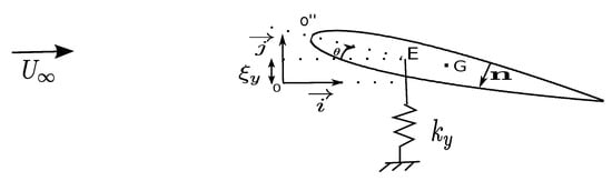
Figure 2. Modeling of the hydrofoil in heave motion with a spring mass system.

The dynamic of the hydrofoil in heave motion is governed by the following equation:

$$m{\ddot{\xi }}_y+k_y{\xi }_y=F_y$$

(12)

with the following initial conditions:

$$\left\{\begin{array}{ccc}\hfill \dot{\xi }\left(0\right)& ={\dot{\xi }}_0\hfill & \hfill \left(a\right)\\ \hfill \xi \left(0\right)& ={\xi }_0\hfill & \hfill \left(b\right)\end{array}\right.$$

(13)

where $F_y$ is the second component of the force vector F (Equation (5)), induced by the fluid flow around the vibrating hydrofoil. Moreover, due to linearity, the solution of Equations (6) and (7) can be expressed as $p_1=-{\ddot{\xi }}_y{p}_1^{\prime }$ and $p_2=-{\dot{\xi }}_y{p}_2^{\prime }$, where $p_1^{\prime }$ and $p_2^{\prime }$ are respectively the solutions of the following systems:

$$\left\{\begin{array}{cccc}\hfill \Delta p_1^{\prime }=& 0\hfill & \mathrm{on} {\Omega }_F\hfill & \left(a\right)\hfill \\ \hfill \nabla p_1^{\prime }·\mathbf{n}=& \rho n_y\hfill & \mathrm{on} {\Gamma }_{FS}\hfill & \left(b\right)\hfill \\ \hfill p_1^{\prime }=& 0\hfill & \mathrm{on} \partial {\Omega }_F\backslash {\Gamma }_{FS}\hfill & \left(c\right)\hfill \end{array}\right.$$

(14)

and

$$\left\{\begin{array}{cccc}\hfill \Delta p_2^{\prime }=& 0\hfill & \mathrm{on} {\Omega }_F\hfill & \left(a\right)\hfill \\ \hfill \nabla p_2^{\prime }·\mathbf{n}=& \frac{\partial \rho }{\partial t}{n}_y\hfill & \mathrm{on} {\Gamma }_{FS}\hfill & \left(b\right)\hfill \\ \hfill p_2^{\prime }=& 0\hfill & \mathrm{on} \partial {\Omega }_F\backslash {\Gamma }_{FS}\hfill & \left(c\right)\hfill \end{array}\right.$$

(15)

It follows that the Lift force $F_y$ is given by

$$F_y=-{\ddot{\xi }}_y{\int }_{{\Gamma }_{FS}}{p}_1^{\prime }{n}_{y}ds-{\dot{\xi }}_y{\int }_{{\Gamma }_{FS}}{p}_2^{\prime }{n}_{y}ds$$

(16)

and Equation (12) can be rewritten as:

$$\left(m+m_a\right){\ddot{\xi }}_y+d_a{\dot{\xi }}_y+k_y{\xi }_y=0$$

(17)

where $m_a$ and $d_a$ are respectively the added mass and added damping,

$$m_a={\int }_{{\Gamma }_{FS}}{p}_1^{\prime }{n}_{y}ds\mathrm{and}{d}_a={\int }_{{\Gamma }_{FS}}{p}_2^{\prime }{n}_{y}ds$$

The coupled problem can thus be reduced to solving the Equations (14), (15) and (17). On the one hand, Equations (14) and (15) give the added mass and added damping (fluid load on the structure). On the other hand, Equation (17) provides the structure dynamics (structure displacement, velocity and acceleration). Note that, for fixed angle of attack ($8^{\circ }$ for our case), $n_y$ has a fixed value and the variation of the solutions $p_1^{\prime }$ and $p_2^{\prime }$ depend only on the density $\rho$ and its variation rate ($\frac{\partial \rho }{\partial t}$).

4. Non-Homogeneous Density Model

Modeling of the density variation is made in order to approximate the sheet cavitation behavior on the hydrofoil, as described in the literature [10,14,15]. Sheet cavitation is characterized by unsteady behavior of cavity length $L_p$ at the hydrofoil upper surface (Figure 3). Attached at the leading edge, the cavity extends on the upper surface and oscillates between the minimum length cavity ($L_{p_{min}}$) to the maximum length ($L_{p_{max}}$). Inside the cavity, the vapor density ${\rho }_v$ is equal to 1 kg/m³. Outside the cavity, the hydrofoil is surrounded by liquid (water) with the density ${\rho }_l$ equal to 1000 kg/m³. At the interface ${\Gamma }_{FS}$, the density $\rho$ is given by

$$\rho (x,y,t)=\left\{\begin{array}{cccc}\hfill {\rho }_v=& 1 {\mathrm{k}\mathrm{g}/\mathrm{m}}^3\hfill & if 0\le x<L_p\left(t\right)\hfill & \hfill \left(a\right)\\ \hfill {\rho }_l=& 1000 {\mathrm{k}\mathrm{g}/\mathrm{m}}^3\hfill & if L_p\left(t\right)\le x<L_{p_{max}}\hfill & \hfill \left(b\right)\end{array}\right.$$

(18)

and the variation rate of the density is given by

$$\left\{\begin{array}{c}\frac{\partial \rho }{\partial t}=({\rho }_v-{\rho }_l)\delta (x-L_p\left(t\right))\frac{\partial L_p\left(t\right)}{\partial t},\hfill \\ 0\le x\le c,(x,y)\in {\Gamma }_{FS}\mathrm{and} L_{p_{min}}\le L_p\left(t\right)\le L_{p_{max}}\hfill \end{array}\right.$$

(19)

where $\delta$ is a Dirac function.

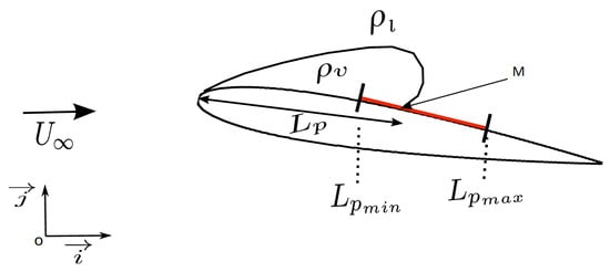
Figure 3. Modeling of sheet cavitation. M oscillation belongs to [$L_{p_{min}}$, $L_{p_{max}}$].

There are different development phases of sheet cavitation. Firstly, the closing point M (Figure 3) has a small variation and the cavity could be considered to be steady. Secondly, the cavity length $L_p$ increases and the closing point oscillates between $L_{p_{min}}$ and $L_{p_{max}}$. The cavitation development phases may continue to the destabilization of the cavity, followed by a vapor cloud detachment [16,17]. In this paper we focus on the first two phases. During the second phase, the cavity length follows a periodic variation [14,18].

Let us consider the following simplified model of unsteady cavity

$$L_p\left(t\right)=L_{p_{min}}+\frac{L_{p_{max}}-L_{p_{min}}}{2}(1-cos\left(2\pi f_{c}t\right))$$

(20)

where $f_c$ is the oscillation frequency of the closing point M. The variation rate of cavity length is given by

$$\frac{\mathrm{d}{L}_p}{\mathrm{d}t}=(L_{p_{max}}-L_{p_{min}})\pi f_{c}sin\left(2\pi f_{c}t\right)$$

(21)

5. Numerical Resolution

A 2D hydrofoil of type NACA0012, with a mass per unit of length (m) equal to 14.505 kg· m⁻¹, is used. Its natural frequency $f_N$ in the air is 58.52 Hz and the chord length c is equal to 0.15 m. The stiffness is deduced from the previous values.

The Newmark scheme [19] presented in Equation (22) is used to discretize the structure dynamics Equation (17). The latter is given by:

$$\left\{\begin{array}{ccc}\hfill {\xi }_y^n=& {\xi }_y^{n-1}+\Delta t{\dot{{\xi }_y}}^{n-1}+\frac{\Delta t^2}{4}({\ddot{{\xi }_y}}^{n-1}+{\ddot{{\xi }_y}}^n)\hfill & \left(\mathit{a}\right)\hfill \\ \hfill {\dot{{\xi }_y}}^n=& {\dot{{\xi }_y}}^{n-1}+\frac{\Delta t}{2}({\ddot{{\xi }_y}}^{n-1}+{\ddot{{\xi }_y}}^n)\hfill & \left(\mathit{b}\right)\hfill \end{array}\right.$$

(22)

where $\Delta t$ is the time step and ${\xi }_y^n$ is the value of the displacement ${\xi }_y$ at time $t_n=n\Delta t$. In this study, the time step is taken equal to ${10}^{-3}$ s, which is a good time sampling of both the hydrofoil harmonic displacements (with a period of about $17\times {10}^{-3}$ s) and the harmonic variations of the cavity (with a period of about $44\times {10}^{-3}$ s).

The problem (fluid and structure) is solved by using the finite elements code CASTEM [20]. Triangular quadratic elements are used. The computational domain is subdivided into 34,360 elements, which corresponds to 131,720 nodes. As shown in Figure 4, the mesh of the subdomain around the hydrofoil is refined in order to improve the accuracy of the numerical results.

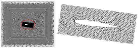
Figure 4. Computational domain and mesh: 34,360 elements and 131,720 nodes (left). Mesh subdomain around the hydrofoil (right).

The same mesh sensitivity study performed in [11] is used here. Figure 5 shows the mesh dependence of the numerical added mass value obtained by solving Equation (14). The chosen mesh corresponds to a relative error of about $1.56\%$, compared to the analytical value of the added mass obtained for a rectangle of the same dimensions as the used hydrofoil [11].

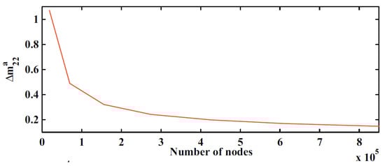
Figure 5. Mesh sensitivity [11].

5.1. Steady Cavity Length

Steady cavity length is first studied in order to understand the effect of cavity length $L_p$ on the structure dynamics. In this case, the cavity length $L_p$ is considered to be constant. Hence, the fluid density is only space dependent and its variation rate is zero. Hence, $\frac{\partial \rho }{\partial t}$ and $p_2^{\prime }$ are equal to zero. It follows that the added mass $m_a$ is constant and the added damping $d_a$ is zero.

The simulation is performed for one value of steady $L_p$ equal to $0.4c$. Only Equations (14) and (17) are solved for the coupled problem. It follows that the induced movement ${\xi }_y$ of the hydrofoil is periodic. Thus, it can be defined by the induced frequency $f_I$ and the corresponding amplitude. The induced frequency $f_I$ of the structure oscillations into the fluid flow can be obtained by Fast Fourier Transform (FFT).

The same study was reproduced for different values of $L_p$ ($L_p=0$ to $L_p=c$). The induced frequencies versus cavity length are presented in Figure 6. It can be shown that the value of $L_p$ does not affect the amplitude of the hydrofoil displacement (Figure 6a). However, the frequency increases according to the cavity length (Figure 6b). This is expected because the surface covered by vapor expands as $L_p$ increases. Furthermore, the added damping $d_a$ is zero because of the steady cavity length. Therefore, the induced frequency $f_I$ can be deduced from Equation (17) as follows:

$$f_I=\frac{1}{2\pi }\sqrt{\frac{k_y}{m+m_a}}$$

(23)

The frequency $f_I$ can be approximated by using the Formula (24) given in [21]

$$\frac{f_I}{f_N}=\frac{1}{{(1+\frac{m_a}{m})}^{\frac{1}{2}}}$$

(24)

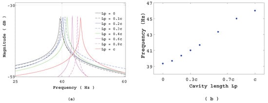
Figure 6. (a) Spectrum of hydrofoil movement ${\xi }_y$ for different values of $L_p$. (b) Frequency of ${\xi }_y$ versus $L_p$.

5.2. Unsteady Cavity Length

The simulation of the coupled problem is now performed with unsteady cavity length. The same values of mass, natural frequency ($f_N$), and chord length used previously are applied. Equation (20) is applied for cavity length oscillation; where $L_{p_{max}}=0.4c$, $L_{p_{min}}=0$ and $f_c=22.5$ Hz. The value of $f_c$ is chosen to be close to the experimental observation [10].

Solutions $p_1^{\prime }$ of Equation (14) in a fluid domain at three different moments, corresponding respectively to $L_p\approx L{p}_{min},L_p\approx \frac{L{p}_{max}}{2}$ and $L_p\approx L{p}_{max}$, are shown in Figure 7 (left). It is easy to see that the values of $p_1^{\prime }$ at the upper surface are smaller than those of the lower surface. Indeed, $p_1^{\prime }$ is proportional to the fluid density and the hydrofoil is surrounded by the vapor at the upper surface.

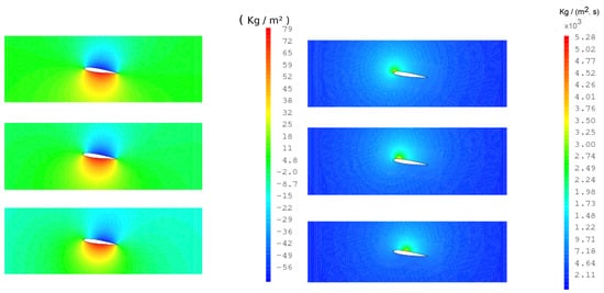
Figure 7. Solutions $p_1^{\prime }$ (left) and $p_2^{\prime }$ (right) for three times corresponding respectively to $L_p\approx L{p}_{min},L_p\approx \frac{L{p}_{max}}{2}$ and $L_p\approx L{p}_{max}$.

Values of $p_2^{\prime }$ at the same three moments, corresponding to the three values of $L_p$, are shown in Figure 7 (right). High values match with the closure points M where the density changes. Indeed, $p_2^{\prime }$ is proportional to the variations rate of the density as shown in Equations (15) and (19), and that formulation includes Dirac function. Therefore, the variations of $L_p$ can be observed within the solution $p_2^{\prime }$. It follows that the added mass $m_a$ is time dependent. Its variation are shown in Figure 8a. It oscillates between $13.92$ kg·m⁻¹ and $17.04$ kg·m⁻¹. These values correspond respectively to values of $L_{p_{max}}$ and $L_{p_{min}}$. The maximum value corresponds to that obtained in the homogeneous fluid case. Hence, it is assumed that the added mass variations is periodic and has the same frequency as the cavity length variation. It can be concluded that a frequency modulation of the structure is expected in this case.

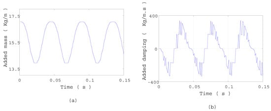
Figure 8. (a) Added mass variation versus time. (b) Added damping variation versus time.

The added damping variation is shown in Figure 8b. It is periodic with a frequency equal to $f_c$ and it can take negative values. It may cause structure instabilities or amplitude modulation.

Hydrofoil motions in both homogeneous and non-homogeneous cases are shown in Figure 9a. The dynamics of the structure are modified by the cavity length oscillation and the phase shift between the two motions increases over time. The spectrum analysis obtained by FFT shows one fundamental frequency centered between two harmonics (Figure 9b). These harmonics specifically characterize an amplitude modulation.

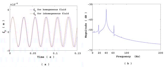
Figure 9. (a) Comparison of hydrofoil displacements in homogeneous and non-homogeneous cases. (b) Frequency of hydrofoil displacements in non-homogeneous case.

The study is reproduced for different values of maximum cavity length ($L_{p_{max}})$. It is shown that the frequency spectrum are still composed by the fundamental frequency and the two harmonics (Table 1). It is noted that the fundamental frequency increases with the cavity length. Variation of the added damping from positive to negative sign and vice versa is observed. This can induce an amplitude modulation of the hydrofoil displacements.

Table 1. Frequencies spectrum of the hydrofoil motion for different $L_{p_{max}}$.

${\mathit{L}}_{{\mathit{p}}_{\mathbf{max}}}$	1st Harmonic (Hz)	Fundamental (Hz)	2nd Harmonic (Hz)
0.2c	17.54	39.47	61.4
0.6c	19.37	41.16	62.95
0.8c	19.22	41.26	63.61
c	17.47	43.67	69.87

5.3. Frequency Analysis

In the previous section, the natural frequency $f_N$ in air, the cavity length $L_{p_{max}}$ and the cavity length frequency $f_c$ were fixed to be close to the experimental observation. However, in this case, the effects of variations in added mass and added damping on the hydrofoil dynamics are difficult to highlight. Indeed, for one period of the hydrofoil oscillation (${\xi }_y$), the cavity length changes from 0 to $\approx L_{p_{max}}/2.6$ and at the same time added mass and added damping vary with the same frequency as the cavity.

Therefore, in order to highlight theses effects, a smaller cavity length frequency $f_c=11$ Hz and a larger cavity length $L_{p_{max}}=0.8c$ are used. It consists of increasing the gap between $f_N$ and $f_c$. The values of c, m, $f_N$ and $L_{p_{min}}$ are the same as in the previous section. The solution of the coupled problem (Equations (14), (15), and (17)) is shown in Figure 10a. An extended analysis performed over a long period of time is reported in Figure 10b. Upper and lower envelopes of the signal ${\xi }_y$ is represented in black curve. This represents the amplitude modulation of the structure dynamics.

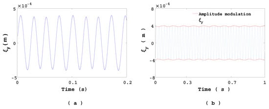
Figure 10. (a) Heave displacement ${\xi }_y$ of the hydrofoil, $t\in [0,0.2]$. (b) Heave displacement ${\xi }_y$ of the hydrofoil over a long period time, $t\in [0,1]$.

To highlight the expected frequency modulation of the structure dynamics, a spectrogram analysis of the signal ${\xi }_y$ is performed. However, an accurate frequency induces automatically a less clearly observable frequency time variation, as shown by Figure 11. This corresponds to the best spectrogram obtained, according to the characteristics presented in Table 2. Indeed, a frequency range is observed and it oscillates with a frequency close to the cavity length variations one. Thus, the classical frequency analysis methods cannot take into account the frequency modulation phenomena. Hence, application of the EMD method followed by the Hilbert spectral analysis are used for the estimation of the instantaneous frequency (IF).

Figure 11. Spectrogram of ${\xi }_y\left(t\right)$ in non-homogeneous case.

Table 2. Spectrogram parameters.

Block Length	Frequency Discretization	Time Lapse between Blocks	Sampling Frequency (Hz)
64	1024	8	1000

5.3.1. Empirical Mode Decomposition

EMD, introduced by Huang et al., is an adaptive and data-driven decomposition well-uited to decompose non-stationary signals derived or not from linear systems [12]. More precisely, no a priori basis functions are required for the decomposition. The algorithm decomposes the multi-component signal into a linear combination of set of reduced number of additive oscillatory components termed as IMFs (Intrinsic Mode Functions). Each extracted IMF, a mono-component signal, must satisfy the following conditions:

(i)

The number of local extrema and the number of zero-crossings must either equal or differ at most by one.

(ii)

The local trend value (mean) of the envelope defined by local maxima and the envelope defined by the local minima is zero

This requirement ensures that the IMFs have no positive local minima and no negative maxima [12]. Furthermore, these conditions allow us to obtain physically meaningful IF estimates from the extracted IMFs. The core of the EMD is called the sifting process and the resulting adaptive expansion can be seen as a type of wavelet decomposition, whose sub-bands are built up as needed to separate the different components of the signal. To be successfully decomposed into IMFs, a signal $s\left(t\right)$ must have at least two extrema: one minimum and one maximum [12,22]. At the end of the sifting, the signal $s\left(t\right)$ can be expanded as the sum of mode time series ${\mathtt{IMF}}_i\left(t\right)$ and a residual $r_K\left(t\right)$:

$$s\left(t\right)=\sum _{i=1}^K{\mathtt{IMF}}_i\left(t\right)+{\mathtt{r}}_K\left(t\right)$$

(25)

where K is the number of modes determined automatically. Based on a dyadic filter bank conjecture of the EMD algorithm, the number of sifted modes K is usually limited to $K\le {log}_2\left(L\right)$, where L is the number of samples of the signal $s\left(t\right)$ [23]. The signal $r_K\left(t\right)$, called residual, is a monotonic function that represents the trend within $s\left(t\right)$.

5.3.2. Hilbert Spectral Analysis

With the extracted modes ${\mathtt{IMF}}_i\left(t\right)$, Hilbert spectral analysis can be applied to each mode in order to estimate the associated IF $f_i\left(t\right)$. To compute the IF, the analytic signal (also called Gabor’s complex signal) associated to a real signal ${\mathtt{IMF}}_i\left(t\right)$ is calculated, as follows

$$\begin{array}{ccc}\hfill z_i\left(t\right)& =& {\mathtt{IMF}}_i\left(t\right)+j\mathcal{H}\left[{\mathtt{IMF}}_i\left(t\right)\right]\hfill \\ & =& a_i\left(t\right)e^{j{\varphi }_i\left(t\right)}\hfill \end{array}$$

(26)

where $a_i\left(t\right)$ and ${\varphi }_i\left(t\right)$ are the instantaneous amplitude and phase of ${\mathtt{IMF}}_i\left(t\right)$. $\mathcal{H}\left[{\mathtt{IMF}}_i\left(t\right)\right]$ is the Hilbert transform of ${\mathtt{IMF}}_i\left(t\right)$ and it is given by

$$\mathcal{H}\left[{\mathtt{IMF}}_i\left(t\right)\right]=\frac{1}{\pi }\mathtt{PV}{\int }_{-\infty }^{+\infty }\frac{{\mathtt{IMF}}_i\left(\tau \right)}{t-\tau }d\tau$$

(27)

where $\mathtt{PV}$ is the Cauchy principal value of the integral. Finally, the IF $f_i\left(t\right)$ of ${\mathtt{IMF}}_i\left(t\right)$ is calculated as follows [24]:

$$\begin{array}{ccc}\hfill f_i\left(t\right)& =& \frac{1}{2\pi }\frac{d{\varphi }_i\left(t\right)}{dt}\hfill \\ \hfill {\varphi }_i\left(t\right)& =& {tan}^{-1}\left(\frac{\mathcal{H}\left[{\mathtt{IMF}}_i\left(t\right)\right]}{{\mathtt{IMF}}_i\left(t\right)}\right)\hfill \end{array}$$

(28)

5.3.3. IMFs and IFs of the Signal ${\xi }_y$

EMD is applied to the signal given by the hydrofoil displacement ${\xi }_y$ and ten IMFs are extracted (Figure 12 and Figure 13). Following EMD definition,

$${\xi }_y\left(t\right)=\sum _{i=1}^{10}{\mathtt{IMF}}_i\left(t\right)+{\mathtt{r}}_{10}\left(t\right)$$

(29)

Here K is set to 10. In our case, two classes of IMFs can be defined: the high frequency class composed by the three first modes and the low frequency composed by the remaining modes. Please note that the first mode, IMF₁(t), corresponds to the highest frequency component of the signal. In our case, it has the highest amplitude for the high frequency class. Zoom of the signal is shown in Figure 14a. Overall, the hydrofoil movement is mainly composed by IMF₁(t) and the remaining low frequency mode.

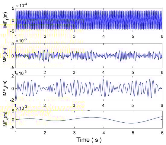
Figure 12. High frequency class: IMF₁, IMF₂, IMF₃ and low frequency class IMF₄ extracted from ${\xi }_y$.

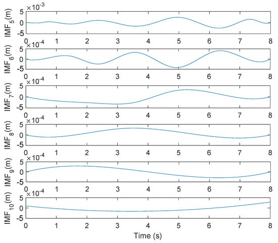
Figure 13. Low frequency class: IMF₅ to IMF₁₀ extracted from ${\xi }_y\left(t\right)$.

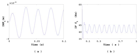
Figure 14. (a) IMF₁(t) mode. (b) IF $f_1\left(t\right)$.

Hilbert spectral analysis of the modes has been performed. The IF $f_1\left(t\right)$ of the first mode (IMF₁(t)), is shown in Figure 14b. The frequency modulation is explicitly shown. Theses oscillations are attributed to the variation of the cavity length. Both variations ($f_1\left(t\right)$ and $L_p$) have the same frequency. The component $f_1\left(t\right)$ oscillates from 39.38 Hz to 44.98 Hz except at the beginning of the simulation.

The IFs of the modes 2 and 3 are shown in Figure 15. They show many peaks (or spikes) which are similar to Dirac functions. If the peaks are omitted, complex oscillation of the IFs $f_2\left(t\right)$ and $f_3\left(t\right)$ are observed. For the low frequency class, the average of IF variations is in the order of ${10}^{-2}$ Hz (Figure 16). It can be concluded that the frequency modulations of the signal ${\xi }_y$ come from the first three IMFs.

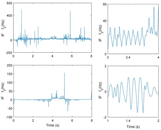
Figure 15. IFs $f_2\left(t\right)$ and $f_3\left(t\right)$ (left), zoom of IFs $f_2\left(t\right)$ and $f_3\left(t\right)$ (right).

Figure 16. IFs from $f_4$(t) to $f_{10}\left(t\right)$.

Some experimental evidence can be found in [15] from experiments conducted on cavitation induced vibration, performed on a hydrofoil in a hydrodynamic tunnel. Typical vibration spectra and the corresponding cavity snapshots on the suction side are shown in Figure 17 for various cavity lengths, according to the cavitation number $\sigma$ obtained on a hydrofoil. The smaller $\sigma$, the larger the maximum cavity length. $\sigma$ is defined as $(P_o-P_v)/\left(0.5\rho U_{\infty }^2\right)$, where $P_o$ is the pressure in the test section and $P_v$ is the vapor pressure [4,10,15,25].

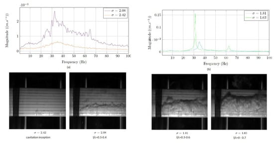
Figure 17. Vibration spectra in cavitating flow and corresponding cavity snapshots on a hydrofoil for various cavitation number: (a) high values of $\sigma$, (b) small values of $\sigma$ [15].

In Figure 17a, $\sigma =2.42$ corresponds to cavitation inception with small spots of vapor attached to the leading edge (bottom of the picture). The corresponding vibration spectrum exhibits a rather large peak corresponding to the structural bending mode. For $\sigma =2.08$, a sheet cavitation was attached at the leading edge and oscillated periodically between about $30\%$ and $40\%$ of the chord length. This leads to an increase of the vibration level over several peaks ranging from about 25 Hz slightly below the bending structural mode frequency at 32 Hz up to the cavity frequency close to 65 Hz. That is the sign of a complex response including frequency modulation probably. As the cavitation number decreases again (Figure 17b, $\sigma =1.81$), the maximum cavity length increases up to $60\%$ of the chord length and oscillates at about 35 Hz close to the structural frequency. By decreasing again the cavitation number ($\sigma =1.63$), the cavity frequency and the bending frequency merge inducing a strong coupling resulting in a very high level resonant peak of vibration at the bending/cavity frequency and harmonics.

6. Conclusions

The effect of the fluid density variations, at the fluid-structure interface, on the structure dynamics is studied and analysed. A decomposition method is used to linearize the fluid-structure coupled problem, which is separated into two components. The first one describes the fluid flow around the fixed hydrofoil while the second one is related to the flow induced by the structure vibrations. A model of the fluid density variation along the upper interface of the hydrofoil, based on the sheet cavitation behaviour, is used. The governing equations are solved numerically using the Finite Element Method. In this study, the hydrofoil is considered to be animated by a free heave motion. For steady cavity length, the added mass remains constant and the added damping (induced by the fluid density rate of change) is zero. The study was reproduced for different values of cavity length. It was highlighted that the frequency increases according to the cavity length. However, the amplitude of the displacement is kept at the same value.

For unsteady cavity length, its oscillations along the fluid-structure interface induces variations in the added mass values. In addition, the fluid density rate of change generates a fluid load acting as an added damping on the structure dynamics, which can be negative and thus at the origin of instabilities of the structure. Although classical methods, such as spectral analysis, make it possible to highlight both amplitude modulation (AM) and frequency modulation (FM) phenomena, in structural dynamics requires the use of suitable tools to handle such AM-FM signals. Thus, empirical mode decomposition (EMD) method, well suited to analyse AM-FM components, was applied to the signal obtained from the hydrofoil displacement. Such a decomposition makes it possible to obtain the instantaneous frequencies (IFs) of the signal from the extracted Intrinsic Mode Functions (IMFs). Therefore, FM is explicitly given through the time variations of the frequency, obtained from EMD method. It is shown that the IF derived from the first IMF, sifted by EMD decomposition of the hydrofoil displacement signal ${\xi }_y$, corresponds to the cavity frequency.

This signal processing method allows us to highlight the FM phenomenon which occurs in the dynamics of a structure immersed in a fluid flow with unsteady non-homogeneous density. In this study, only the effects of the added mass and added damping (induced by the fluid density rate of change) on the structure dynamics are analysed. As future work, we plan to extend this study in order to investigate the potential of the EMD method in this case, by analysing the information and the related physics, which could be extracted from all the sifted IMFs and the associated IFs.

References

- Morand, H.J.P.; Ohayon, R. Fluid Structure Interaction; John Wiley: Hoboken, NJ, USA, 1995. [Google Scholar]
- Axisa, F. Modélisation des Systèmes Mécaniques: Interactions Fluide-Structure; Hermès Science Publ.: Paris, France, 2001. [Google Scholar]
- Sigrist, J.F. Fluid-Structure Interaction: An Introduction to Finite Element Coupling; John Wiley & Sons: Hoboken, NJ, USA, 2015. [Google Scholar]
- Coutier-Delgosha, O.; Stutz, B.; Vabre, A.; Legoupil, S. Analysis of cavitating flow structure by experimental and numerical investigations. J. Fluid Mech. 2007, 578, 171–222. [Google Scholar] [CrossRef]
- Ross, M.R.; Felippa, C.A.; Park, K.; Sprague, M.A. Treatment of acoustic fluid-structure interaction by localized Lagrange multipliers: Formulation. Comput. Methods Appl. Mech. Eng. 2008, 197, 3057–3079. [Google Scholar] [CrossRef]
- Ross, M.R.; Sprague, M.A.; Felippa, C.A.; Park, K. Treatment of acoustic fluid-structure interaction by localized Lagrange multipliers and comparison to alternative interface-coupling methods. Comput. Methods Appl. Mech. Eng. 2009, 198, 986–1005. [Google Scholar] [CrossRef]
- Young, Y. Time-dependent hydroelastic analysis of cavitating propulsors. J. Fluids Struct. 2007, 23, 269–295. [Google Scholar] [CrossRef]
- Young, Y. Fluid-structure interaction analysis of flexible composite marine propellers. J. Fluids Struct. 2008, 24, 799–818. [Google Scholar] [CrossRef]
- Amromin, E.; Kovinskaya, S. Vibration of cavitating elastic wing in a periodically perturbed flow: Excitation of subharmonics. J. Fluids Struct. 2000, 14, 735–751. [Google Scholar] [CrossRef]
- Benaouicha, M.; Astolfi, J.; Ducoin, A.; Frikha, S.; Coutier-Delgosha, O. A numerical study of cavitation induced vibration. In Proceedings of the ASME 2010 Pressure Vessels and Piping Division/PVP Conference, Bellevue, WA, USA, 18–22 July 2010. [Google Scholar]
- Benaouicha, M.; Astolfi, J.A. Analysis of added mass in cavitating flow. J. Fluids Struct. 2012, 31, 30–48. [Google Scholar] [CrossRef]
- Huang, E.N.; Shen, Z.; Long, S.R.; Wu, M.C.; Shih, H.H.; Zheng, Q.; Yen, N.-C.; Tung, C.C.; Liu, H.H. The empirical mode decomposition and the hilbert spectrum for non-linear and non-stationary times series analysis. Proc. R. Soc. 1998, 454, 903–995. [Google Scholar] [CrossRef]
- Benaouicha, M.; Astolfi, J. On Some Aspects of Fluid-Structure Interaction in Two-Phase Flow. In Proceedings of the ASME 2013 Pressure Vessels and Piping Conference, Paris, France, 14–18 July 2013; p. 9. [Google Scholar]
- Leroux, J.B.; Coutier-Delgosha, O.; Astolfi, J.A. A joint experimental and numerical study of mechanisms associated to instability of partial cavitation on two-dimensional hydrofoil. Phys. Fluids 2005, 17, 52–101. [Google Scholar] [CrossRef]
- Astolfi, J.A. Some Aspects of Experimental Investigations of Fluid Induced Vibration in a Hydrodynamic Tunnel for Naval Applications. In Flinovia-Flow Induced Noise and Vibration Issues and Aspects-III; Ciappi, E., De Rosa, S., Franco, F., Hambric, S.A., Leung, R.C.K., Clair, V., Maxit, L., Totaro, N., Eds.; Springer: Berlin/Heidelberg, Germany, 2021; ISBN 978-3-030-64806-0. [Google Scholar]
- Stutz, B.; Reboud, J. Experiments on unsteady cavitation. Exp. Fluids 1997, 22, 191–198. [Google Scholar] [CrossRef]
- Joussellin, F.; Delannoy, Y.; Sauvage-Boutar, E.; Goirand, B. Experimental investigations on unsteady attached cavities. Cavitation ASME-FED 1991, 91, 61–66. [Google Scholar]
- Frikha, S. Étude Numérique et Expérimentale Des écoulements Cavitants sur Corps Portants. Ph.D. Thesis, Arts et Métiers ParisTech, Lille, France, 2010. [Google Scholar]
- Kane, C.; Marsden, J.; Ortiz, M.; West, M. Variational integrators and the Newmark algorithm for conservative and dissipative mechanical systems. Int. J. Numer. Methods Eng. 2000, 49, 1295–1325. [Google Scholar] [CrossRef]
- Combescure, A.; Hoffmann, A.; Pasquet, P. The CASTEM finite element system. In Finite Element Systems; Springer: Berlin/Heidelberg, Germany, 1982; pp. 115–125. [Google Scholar]
- Blevins, R. Formulas for Natural Frequency and Mode Shape; Van Nostrand Reinhold: New York, NY, USA, 1979. [Google Scholar]
- Boudraa, A.; Cexus, J. EMD-based signal filtering. IEEE Trans. Instrum. Meas. 2007, 56, 1597–1611. [Google Scholar] [CrossRef]
- Wu, Z.; Huang, N. A Study of the characteristics of white noise using the empirical mode decomposition method. Proc. R. Soc. Lond. A 2004, 460, 1597–1611. [Google Scholar] [CrossRef]
- Boashash, B.P. Estimating and interpreting the instantaneous frequency of a signal. Part I: Fundamentals. Proc. IEEE 1992, 80, 520–538. [Google Scholar] [CrossRef]
- Balyts’ Kyi, O.I.; Chmiel, J.; Krause, P.; Niekrasz, J.; Maciag, M. Role of hydrogen in the cavitation fracture of 45 steel in lubricating media. Mater. Sci. 2009, 45, 651. [Google Scholar] [CrossRef]
Publisher’s Note: MDPI stays neutral with regard to jurisdictional claims in published maps and institutional affiliations. |
© 2021 by the authors. Licensee MDPI, Basel, Switzerland. This article is an open access article distributed under the terms and conditions of the Creative Commons Attribution (CC BY) license (http://creativecommons.org/licenses/by/4.0/).