Anguilliform Locomotion across a Natural Range of Swimming Speeds

Abstract

Eel-like fish can exhibit efficient swimming with comparatively low metabolic cost by utilizing sub-ambient pressure areas in the trough of body waves to generate thrust, effectively pulling themselves through the surrounding water. While this is understood at the fish’s preferred swimming speed, little is known about the mechanism over a full range of natural swimming speeds. We compared the swimming kinematics, hydrodynamics, and metabolic activity of juvenile coral catfish (Plotosus lineatus) across relative swimming speeds spanning two orders of magnitude from 0.2 to 2.0 body lengths (BL) per second. We used experimentally derived velocity fields to compute pressure fields and components of thrust along the body. At low speeds, thrust was primarily generated through positive pressure pushing forces. In contrast, increasing swimming speeds caused a shift in the recruitment of push and pull propulsive forces whereby sub-ambient pressure gradients contributed up to 87% of the total thrust produced during one tail-beat cycle past 0.5 BL s⁻¹. This shift in thrust production corresponded to a sharp decline in the overall cost of transport and suggests that pull-dominated thrust in anguilliform swimmers is subject to a minimum threshold below which drag-based mechanisms are less effective.

1. Introduction

Anguilliform locomotion is widely regarded as an energetically efficient swimming mode due to the relatively low cost of transportation (COT) during steady swimming [1,2,3]. Early assessments of swimming efficiency generally involved the study of (1) swimming kinematics in relation to muscle activity [4,5,6,7] and (2) metabolic functions (i.e., oxygen consumption and the COT) [1,8,9,10]. This provided valuable information to advancing our understanding of swimming biomechanics, but these methods alone do not provide a complete mechanistic explanation. To do so requires quantifying the underlying animal-fluid interactions driving energy-efficient swimming behaviors. Since complex locomotor behaviors and the implementation of multiple control surfaces for swimming can make mathematical modelling efforts immensely challenging, direct empirical measurements of the flow around the body of a swimming fish represent a means to accurately determine the role of body kinematics and the resulting hydrodynamics in thrust production. This particularly applies when trying to disentangle thrust from drag forces, thus involving the careful consideration of the partitioning of these forces.

Spatially and temporally resolved flow data obtained using methods such as particle image velocimetry (PIV) or other flow visualization methods have greatly enhanced our understanding of fish locomotion [11,12,13,14,15]. Recent advances in computing and experimental techniques now allow for the calculation of high-resolution vorticity and pressure fields from experimentally derived velocity fields [15,16]. While vorticity fields inform us on the structure of the flow near the body of a swimming fish, pressure fields are needed to calculate the magnitude and distribution of the forces acting at the animal-fluid interface. These non-invasive methods broaden the range of tools available to obtain pressure data experimentally with high spatial and temporal resolution. When applied to juvenile sea lampreys (Petromyzon marinus) swimming steadily at their preferred swimming speed, these methods revealed the importance of the thrust forces produced by the pressure difference on either side of the body. Specifically, the pressure gradient formed by the strong sub-ambient pressure areas forming in the trough of a body wave generate a suction-dominated thrust mechanism or “pull thrust” [17,18].

Previous studies investigating the relationship that exists between body kinematics and the formation of thrust-producing near-body hydrodynamics have recognized that the coordinated bending of the body is critical to producing and organizing vorticity along the body of a swimming fish to generate thrust efficiently [19,20]. These bends are responsible for the creation of low-pressure regions, effectively pulling the animals through water [17,18,21]. Although the mechanism driving the production of pull thrust is understood, the energetic benefits remain unclear. Furthermore, research to date on eel-like swimmers has focused only on a narrow range within the naturally achievable swimming speeds and Reynolds numbers. The swimming speeds achieved by anguilliform swimmers in natural settings spans two orders of magnitude and can deviate from their preferred speed and/or optimal speed (COT at its lowest) by up to three times [2,22]. As a result, we do not currently have the information needed to evaluate the limitations and energetics of sub-ambient pressure dominated pull thrust.

For example, are alterations in COT associated with fluctuations in the ratio of pull to push thrust? In this study, we quantify how the active control of body kinematics over a range of natural steady swimming speeds is related to changes in the overall contribution of sub-ambient pressures (pull forces) and high pressures (push forces). Additionally, we investigated how the distribution of the push and pull components of thrust along the body varied with changes in swimming kinematics. We also explored the metabolic advantage of using pull-dominated thrust as opposed to reactive push forces to achieve a low COT, and thus to optimize swimming efficiency. To experimentally evaluate this, we investigated metabolic activity, swimming kinematics, and experimentally derived pressure fields and force vectors in an eel-like swimmer, the coral catfish (Plotosus lineatus), as the fish swam at different steady velocities spanning two orders of magnitude. We discuss these results in the context of the dynamics and relative contribution of both reactive and pull forces to total thrust and metabolic activity.

2. Materials and Methods

2.1. Ethics Statement

This study was conducted in accordance with the laws of the State of Florida and under IACUC protocols (Permit # IS00005965) approved by the University of South Florida (Tampa, FL, USA).

2.2. Animals

Coral Catfish (Plotosus lineatus) (number of fish = 7; body length = 0.074 ± 0.003 m; mass = 1.51 ± 0.10 g) were selected because of their ubiquitous reliance on eel-like body undulations, relative steadiness across a range of swimming speeds and relatively small body size for the swim tunnel respirometer. The fish were maintained in an aerated 150-L aquarium at 26 °C, salinity of 30% and 12 h:12 h light: dark photoperiod. The fish were fed daily to satiation but were fasted for 24 h prior to any experiment so that metabolic measurements were obtained in a post-absorptive state. Standard body length (BL) was measured digitally along the midline of each specimen from scaled dorsal view images of the fish using ImageJ software. The lateral profile of the fish was also established using scaled lateral view images (Figure S1). The wet mass of the fish was measured in vivo using a precision balance (Carolina, Burlington, NC, USA).

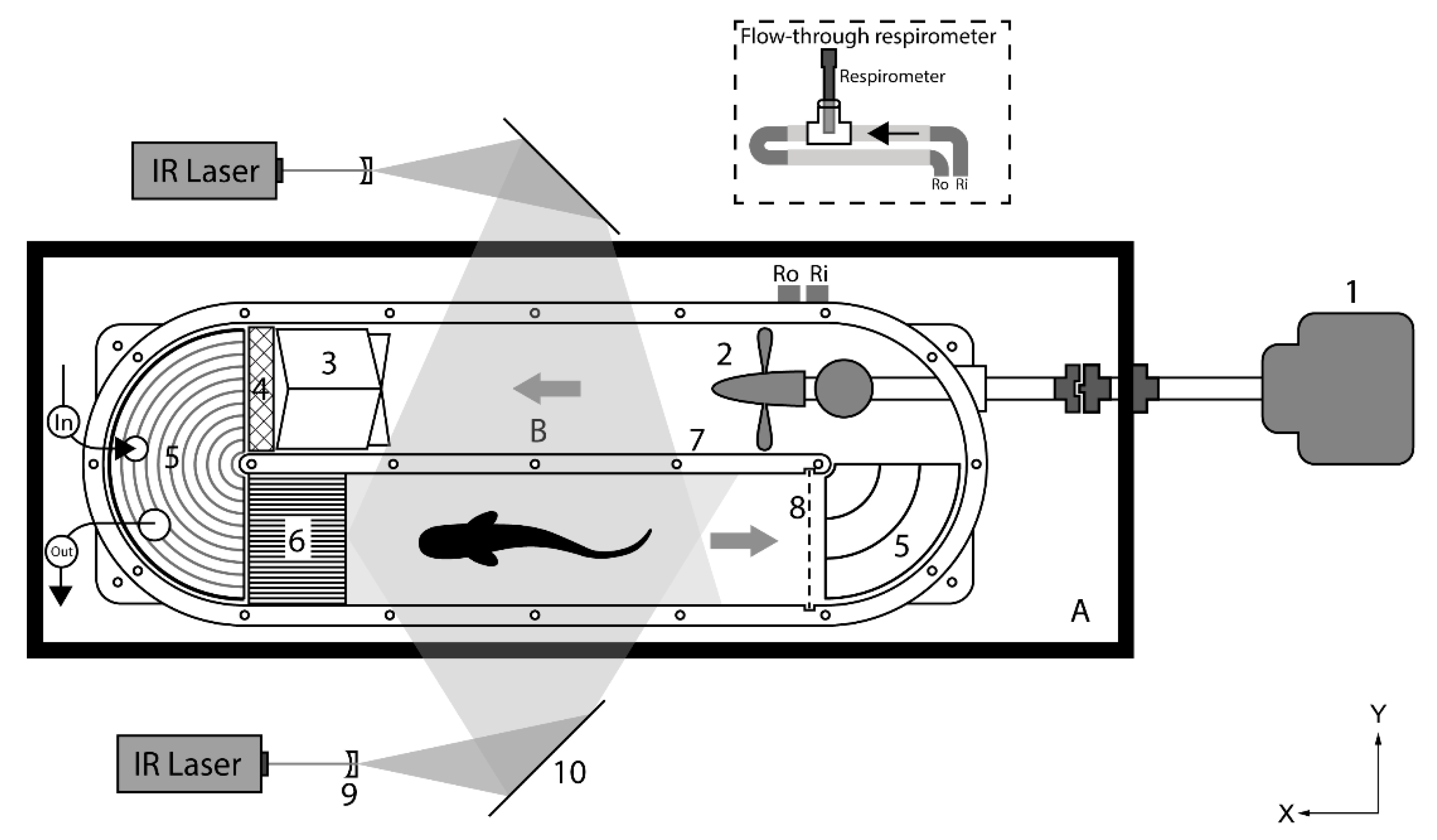
2.3. Experimental Setup

2.3.1. Swim Tunnel Respirometer

Flow visualization and respirometry experiments were conducted in a modified 5-L Brett-type swim tunnel respirometer (Loligo Systems, Viborg, Denmark) (Figure 1). The working section of the swim tunnel was 0.30 × 0.075 × 0.075 m (length × width × depth). The respirometer was submerged in an aerated outer buffer tank maintained at ambient temperature (21 ± 1.0 °C) that provided aerated water when flushing the swim tunnel respirometer after each closed measuring period (flush pump, Eheim, Deizisau, Germany, 0.01 m³ min⁻¹). For respirometry experiments, an additional external flow-through respirometer loop was connected to the swim tunnel. The calibration of water flow velocity to voltage output from the external motor driving the impeller generating the flow in the respirometer was performed using PIV. Additionally, flow characteristics were assessed using PIV to ensure a uniform velocity profile throughout the cross-sectional area of the test section (see Figures S2 and S3).

2.3.2. Respirometry

Relative oxygen consumption rates (ṀO₂) of coral catfish (number of fish = 7) were measured for swimming speeds ranging from 0.2 BL s⁻¹ to 2.0 BL s⁻¹. Intermittent flow respirometry was employed based on a protocol derived from existing methods [23] to limit risks of hypoxia and hypercapnia. Each fish transferred to the test section of the respirometer was allowed to recover from handling at a swimming speed ≤0.3 BL s⁻¹ and with fully aerated and thermoregulated seawater from the buffer tank (continuous flushing phase) for 4 h prior to starting the experiment. The duration of this recovery period was established from the decline in the measured resting metabolic rate over time that reached an asymptote about four hours after the fish were placed in the swim tunnel (see Figure S4). Temperature-corrected dissolved oxygen concentration was measured in mg L⁻¹ at a sampling frequency of 1 s⁻¹ using an optical oxygen dipping probe (PreSens, DP-PSt3, Regensburg, Germany) connected to a fiber optic oxygen transmitter (PreSens, OXY-1 SMA, Regensburg, Germany) interfaced to a computer.

One complete closed-phase cycle for each swimming speed consisted of three distinct timing periods: (1) a flush period during which oxygen saturation was brought to 100%, and the fish was allowed to rest at a swimming speed ≤0.3 BL s⁻¹ for 30 min; (2) a short wait period of 1 min during which the swim tunnel respirometer was sealed and the desired flow speed established; and (3) a measurement period of 10 min (for all swimming speeds) during which ṀO₂ was measured. The rate of oxygen consumption was calculated as follows:

$${\mathrm{Ṁ}\mathrm{O}}_2=\frac{\left(∆\left[{\mathrm{O}}_2\right]-∆{\left[{\mathrm{O}}_2\right]}_{\mathrm{background}}\right)\times V}{\mathrm{m}}$$

(1)

where oxygen consumption ṀO₂ is measured in mg min⁻¹ kg⁻¹, ∆[O₂] is the total decline in oxygen concentration in the swim tunnel respirometer over a measurement period of 10 min, ∆[O₂]_background is the change in oxygen concentration due to bacterial background respiration over a measurement period of 10 min, V is the respirometer water volume (5.48 × 10⁻³ m³), m is the mass of the fish in kg. ∆[O₂]_background over a measurement period of 10 min did not exceed 0.01 mg L⁻¹. Resting oxygen consumption rate (ṀO_2,resting) was measured for 10 min under dim illumination conditions in a smaller resting respirometer chamber (3.95 × 10⁻⁴ m³) that prevented the fish from swimming actively against the flow. COT (J m⁻¹ kg⁻¹) serves as a measure of swimming efficiency and was calculated using ṀO₂ and ṀO_2,resting as follows:

$$\mathrm{COT}=\frac{{\mathrm{Ṁ}\mathrm{O}}_2-{\mathrm{Ṁ}\mathrm{O}}_{2\mathrm{resting}}}{\mathrm{U}}$$

(2)

where U is the swimming speed in m min⁻¹ at each velocity increment. Conversion of metabolic respiration to energy expended (joules) is accomplished by using the oxy-calorific equivalent of 3.24 cal mg⁻¹ of O₂ measured for carnivorous fish [24] and the standard thermochemical conversion factor 4.184 J cal⁻¹.

2.3.3. PIV Experiments

Three-dimensional velocimetry methods are powerful tools in the investigation of swimming hydrodynamics away from the body, particularly when studying the wake [25]. However, here we used 2D PIV for its greater accuracy in capturing velocities adjacent to moving surfaces [26]. Since this investigation focused on near-body hydrodynamics, the accurate measurement of velocities at the animal-fluid interface was paramount to producing reliable pressure fields from which the calculations of the forces acting on the body were derived. Although 2D PIV cannot account for out-of-plane velocities, validations of this method have demonstrated that it performs well when in-plane velocities dominate thrust production [15,16]. The investigation of the horizontal divergence of the vector fields in the x-y plane along the rostro-caudal axis and above the rostro-caudal axis (along the dorsal fin) revealed no identifiable 3D flow structures along the majority of the length of the body of the fish (see Figure S5).

Recordings (3 s) were acquired at 500 frames s⁻¹ using an Edgertronic SC1 high-speed camera with a resolution of 1280 × 1024 pixels (Edgertronic, San Jose, CA, USA). Analogous to the methods described by [21], 20 µm Polyamid seeding particles (Dantec dynamics, Skovlunde, Denmark) were illuminated by two opposing overlapping horizontal laser sheets produced by two continuous wave 808 nm lasers (MDL-H-808 3000–6000 mW, OptoEngine LLC, Midvale, UT, USA) to eliminate shadows on either side of the fish. During the closed filming period, no water flow between the buffer tank and the swim tunnel was allowed in order to maintain the seeding density of the water in the test section constant, and to limit additional scattering of the light. The filming period did not exceed 60 min and oxygen levels were not allowed to fall below 75% oxygen saturation. Swimming speeds ranging from 0.2 BL s⁻¹ to 2.0 BL s⁻¹ were investigated.

2.4. Kinematics, Pressure, and Force Calculations

A custom program in MATLAB R2018a (MathWorks, Natick, MA, USA) was used to automatically identify the outline of the fish from the raw image sequences based on the difference in contrast at the animal-fluid interface. The raw outlines of the animal were smoothed and were used to construct the midline of the fish onto which 6 evenly spaced points were identified (1 and 6 representing the snout at 0 BL and the tip of the tail at 1 BL respectively). The outlines were also used in the calculation of vorticity and pressure fields and force components [16]. The width of the amplitude envelope identified over the course of one complete tail beat was calculated to determine the maximum lateral displacement of the body at each of the points identified along the midline. Tail-beat frequency f was measured in s⁻¹ at the tip of the tail and was averaged over 3 complete tail-beat cycles for each swimming speed increment for all fish. Additional kinematic parameters including wavelength, period, and body-wave speed were calculated from the midlines. Wavelength and body-wave speed were normalized to body length. The slip, the Strouhal number (St), and the Reynolds number (Re) were calculated using the previous parameters [13].

Fluid velocity vectors were calculated from sequential images analyzed using the DaVis 8.3 software package (LaVision, Göttingen, Germany). Only the sequences during which the fish were swimming within the center of the flume (relative to the y and z axes) were considered for analysis. Image pairs were analyzed with three passes of overlapping interrogation windows (50%) of decreasing size yielding 64 × 80 vectors per frame. Every two frames were used for analysis, yielding a separation between frames (dt) of 4 × 10⁻³ s. Vorticity fields were calculated for every two velocity fields, yielding a total separation between frames of 8 × 10⁻³ s using the built-in function available in MATLAB R2018a. Due to the two-dimensional nature of the velocity fields, only the vertical component of vorticity was calculated [27]. Pressure fields were calculated with the same separation increments, using the queen 2.0 pressure field package for MATLAB available at: http://dabirilab.com/software (Accessed on: 18 October 2019). The algorithm integrates the Navier—Stokes equation for each velocity point in the field of view, and the pressure at each point is determined by computing the median pressure from eight integration paths emanating from each point. This method has been previously evaluated and validated against experimental and computational data, including simulations of anguilliform swimming [15] and was demonstrated to be appropriate for the study of fish locomotion [17,18,21]. However, more recent computation methods aiming at reducing the error propagation present new avenues for more accurate computations of experimentally derived pressure fields [28]. Pressure fields were subsequently used to calculate thrust and drag forces per height along fifty evenly sized segments around the body by multiplying the pressure measured at the boundary of the fish by the vector normal to the surface and the unit vector in the x-axis (direction of swimming) [16,18]. Thrust forces are positive and drag forces are negative. To simplify terminology, forces were classified as pull and push forces when arising from sub-ambient pressures (negative relative to ambient) and above-ambient pressures (positive), respectively. To account for the effects of changes in body depth along the length of the fish on the total magnitude of thrust and drag, a normalized depth profile was produced along 12 equally distributed body segments from the digitized lateral outline of a fish (Figure S1). Values for the pull and push components of drag and thrust were then multiplied by the depth at each body segment. This method assumes a uniform pressure profile along the height of the fish and may not fully capture the effects of three-dimensional flow. However, when out-of-plane flows are negligible compared to the planar flow and when pressure effects dominate shear effects, this technique is able to accurately reproduce the direction, magnitude, and timing of locomotor forces experienced by a fish [16].

2.5. Statistics

All statistical tests were performed using MATLAB R2018a. ANOVA F-test was used to test for significant differences in kinematics parameters between swimming speeds, and Tukey’s post hoc tests were used to determine which group means were significantly different from other group means and to control the experiment-wise error rate [29]. Differences were considered significant at p-values less than α = 0.05. Parameters are reported as means plus or minus standard deviations. For linear associations between swimming speed and kinematics parameters, Pearson correlation analyses were performed [29]. The coefficient of determination R² and Pearson correlation coefficient r were calculated for each regression. Differences were regarded as statistically significant at p < 0.01. A two-way repeated measure analysis of variance (ANOVA) was conducted with speed and location along the body as the two main effects for body lateral displacement [29]. We used the two-way ANOVA procedure to calculate the type III sums of square used in the ANOVA. Tukey’s post hoc comparisons were conducted, and again, we used the 0.05 probability level as our criterion for statistical significance [29].

3. Results

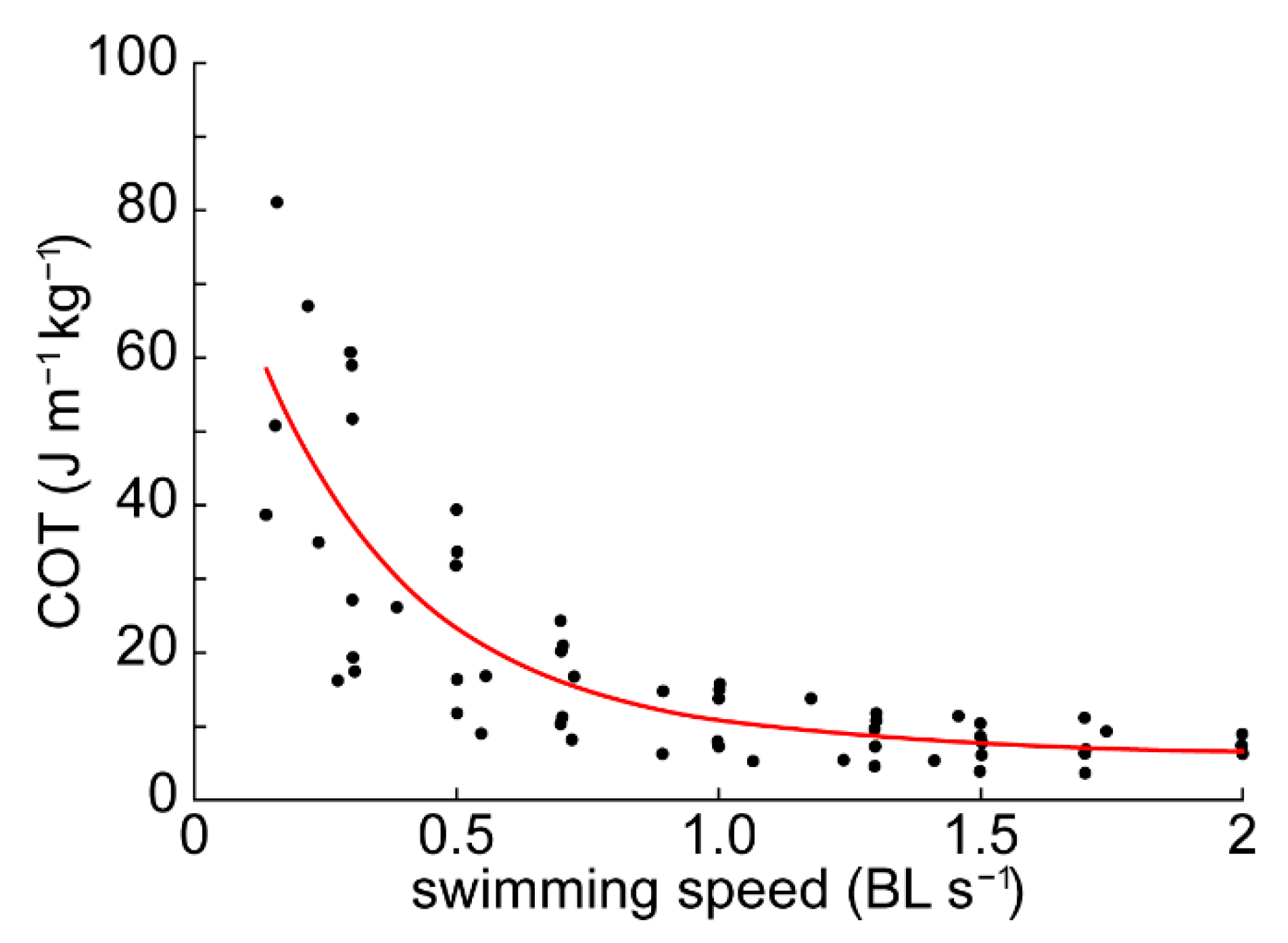
3.1. Cost of Transport

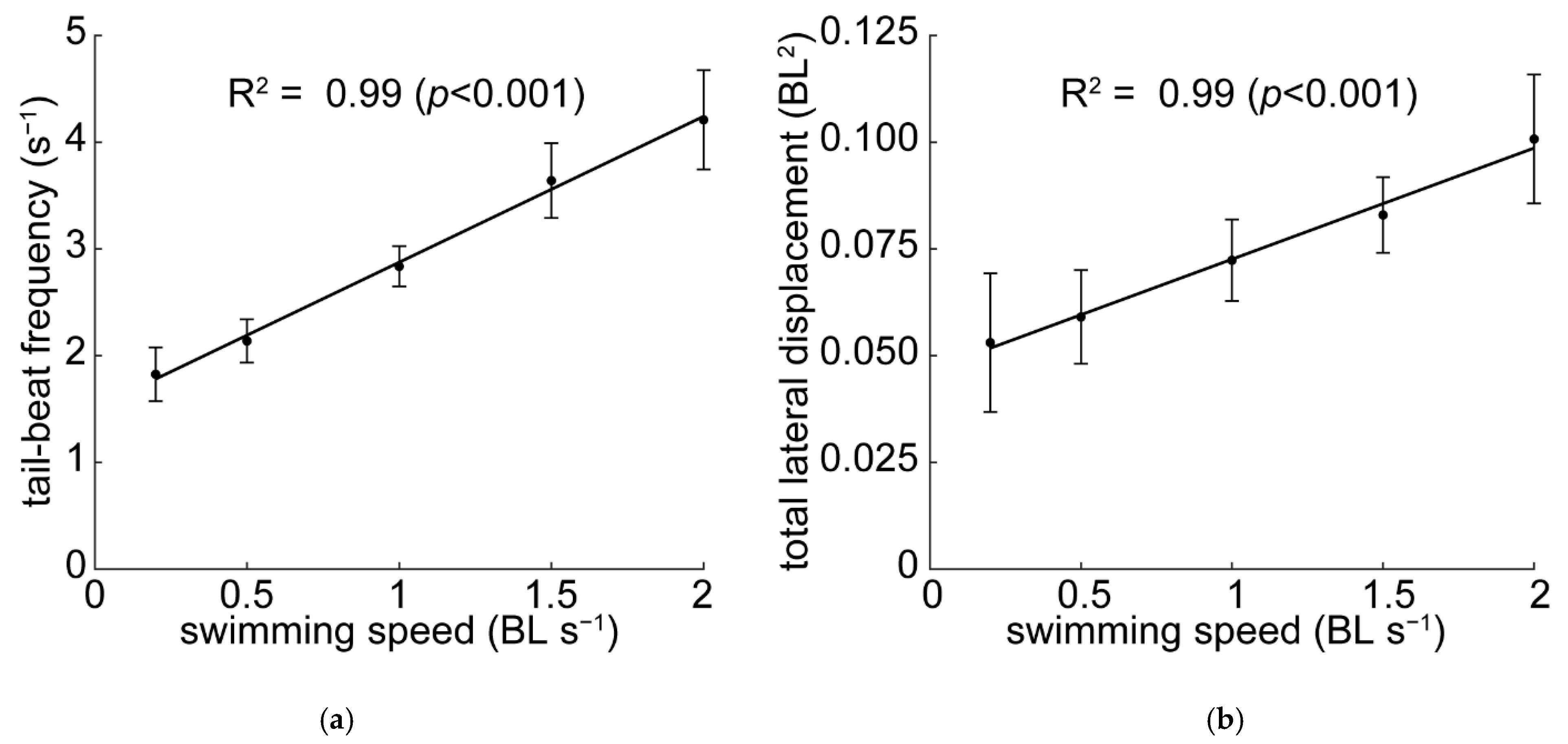
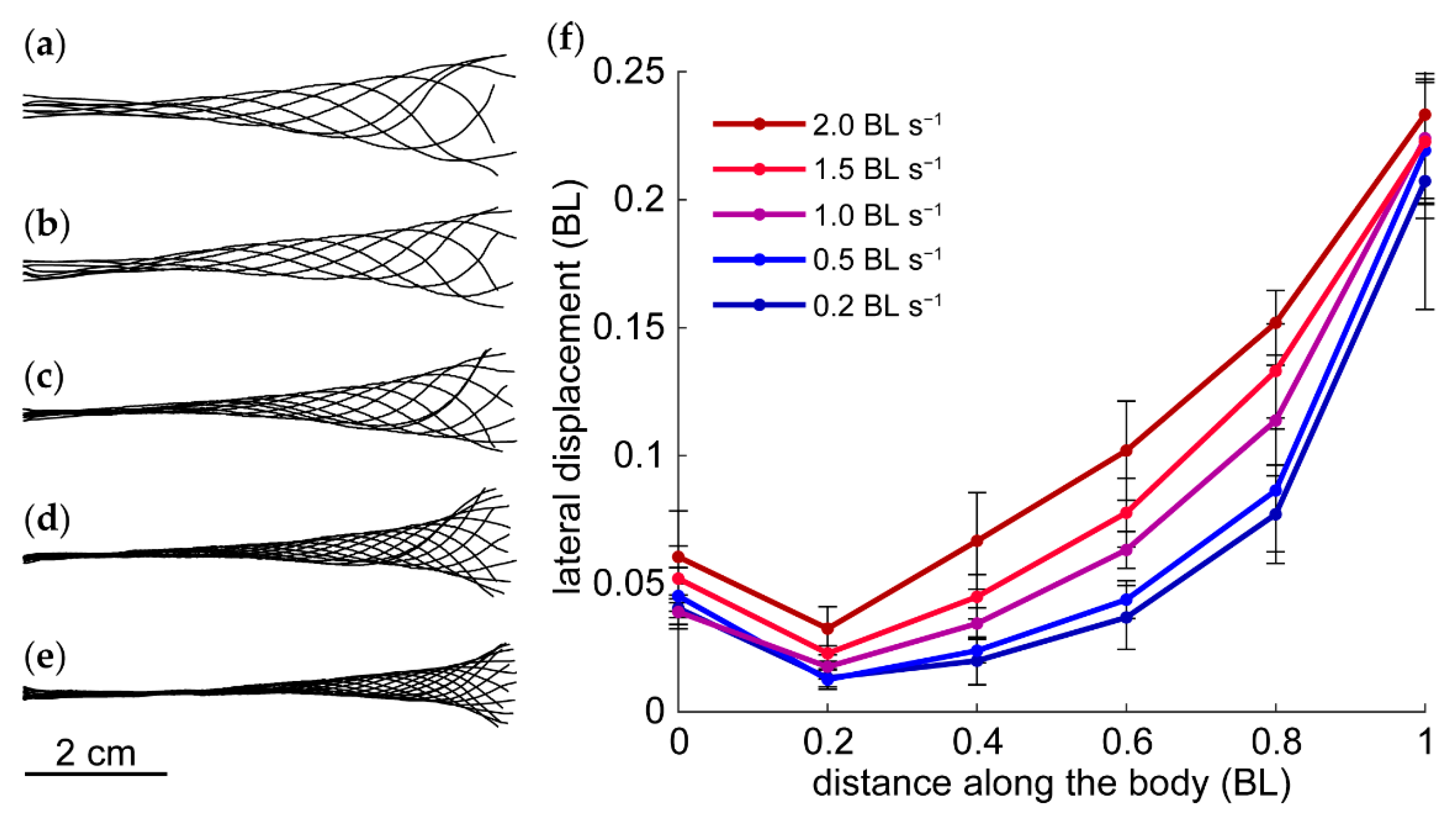
The metabolic cost of swimming was measured as the COT at given swimming speeds (U) ranging from 0.14 to 2.0 BL s⁻¹. It should be noted that 2.0 BL s⁻¹ was the maximum sustained speed that P. lineatus exhibited. The COT of steadily swimming fish decreased with increasing swimming speed and was lowest at 2.0 BL s⁻¹ (COT = 6.47 ± 2.15 J m⁻¹ kg⁻¹) (Figure 2). The slope of the J-shaped curve fitted to the data was greatest for speeds <0.5 BL s⁻¹, and the COT for such swimming speeds was up to 10 times that of the COT calculated at speeds >1.0 BL s⁻¹.

3.2. Kinematics

Tail-beat frequency (f), measured at the tip of the tail during steady swimming (U), showed a strong linear association with swimming speeds ranging from 0.2 BL s⁻¹ to 2.0 BL s⁻¹ (R² = 0.997; r = 0.998; p < 0.01) (Figure 3a and

Table 1. Kinematic parameters. Means ± s.d. of kinematic parameters for steady swimming at speeds ranging from 0.2 to 2.0 BL s⁻¹ and p-value results of ANOVA F-test (number of fish = 7). Parameters showing no significant difference across swimming speeds are indicated with the same superscript letters.

Parameters	Symbols	Units	0.2 BL s−1	0.5 BL s−1	1.0 BL s−1	1.5 BL s−1	2.0 BL s−1	p-Value
Reynolds number	Re		1319 ± 406	2767 ± 316	5430 ± 556	8152 ± 782	10,835 ± 1033	<0.05
amplitude envelope area	A	BL2	0.05 ± 0.01	0.06 ± 0.01	0.07 ± 0.01	0.08 ± 0.013	0.10 ± 0.01	<0.05
wavelength	λ	BL	0.62 ± 0.01	0.68 ± 0.02	0.71 ± 0.02	0.73 ± 0.01	0.75 ± 0.01	<0.05
period	T	s	0.55 ± 0.04	0.47 ± 0.02	0.35 ± 0.01	0.28 ± 0.01	0.24 ± 0.01	<0.05
frequency	f	s−1	1.83 ± 0.14	2.14 ± 0.08	2.84 ± 0.08	3.64 ± 0.13	4.21 ± 0.18	<0.05
body-wave speed	V	BL s−1	1.14 ± 0.09	1.45 ± 0.04	2.01 ± 0.08	2.67 ± 0.09	3.16 ± 0.13	<0.05
slip			0.18 ± 0.01	0.35 ± 0.01	0.50 ± 0.02	0.57 ± 0.02	0.64 ± 0.03	<0.05
Strouhal number	St		1.88 ± 0.23	0.93 ± 0.03	0.63 ± 0.02	0.54 ± 0.01	0.49 ± 0.02	<0.05

). The maximum tail-beat frequency of 4.21 ± 0.18 s⁻¹ was achieved by the fish upon reaching their maximum sustained speed U_max = 2.0 BL s⁻¹ past which they could not reliably hold stationary against the flow.

The total area of lateral displacement of the body (normalized to BL²) as a body wave traveled along the body during one complete tail-beat cycle was expressed here as the amplitude envelope area (A) between the outermost bounds of the centerlines obtained from each frame. It showed a strong linear association with swimming speed (R² = 0.991; r = 0.995; p < 0.01) (Figure 3b and Table 1). The superimposed centerlines traced for each swimming speed over one complete tail beat revealed that the overall width of the amplitude envelope increased along the body with increasing swimming speed, particularly anteriorly to the tip of the tail (Figure 4a–e). The body waves were generated posteriorly to the head of the fish at a distance of about 0.2 BL from the tip of the snout (Figure 4f). At 0.2 and 0.5 BL s⁻¹, pronounced body undulations were mostly confined to the posterior-most section of the tail located between 0.6 and 1 BL, as indicated by the curved outer boundaries of the amplitude envelope (Figure 4d,e). This reveals that the amplitude of the body waves did not increase steadily along the entire length of the fish. In contrast, for speeds ≥1.0 BL s⁻¹ the amplitude of the body waves increased more steadily along the entire length of the body as indicated by the straight outer edges of the amplitude envelopes (Figure 4a–c). This translated to an increase in the magnitude of the lateral displacement of the body more anteriorly with increasing swimming velocities (Figure 4f). These changes were accompanied with an overall increase in the wavelength of the body waves from 0.62 ± 0.01 BL at 0.2 BL s⁻¹ to 0.75 ± 0.01 BL at 2.0 BL s⁻¹ (p < 0.05). This indicates that more of the body was solicited in the production of propulsive body waves with increasing swimming speeds.

Additionally, changes in the magnitude of the lateral displacement across swimming speeds showed the greatest significance at sections of the body located between 0.4 and 0.8 BL (p < 0.05). Interestingly, despite this increased involvement of the anterior section of the body in wave production and circulation, the change in the magnitude of the lateral displacement of the tip of the tail was not significant across all swimming speeds (p > 0.05). Overall, changes in lateral displacement of the body were strongly correlated with swimming speed (p < 0.001) as well as with the location along the body (p < 0.001). Further, body lateral displacement had a highly significant interaction term between speed and site along the body (p < 0.005), thus indicating a strong correlation between body kinematics and swimming speed.

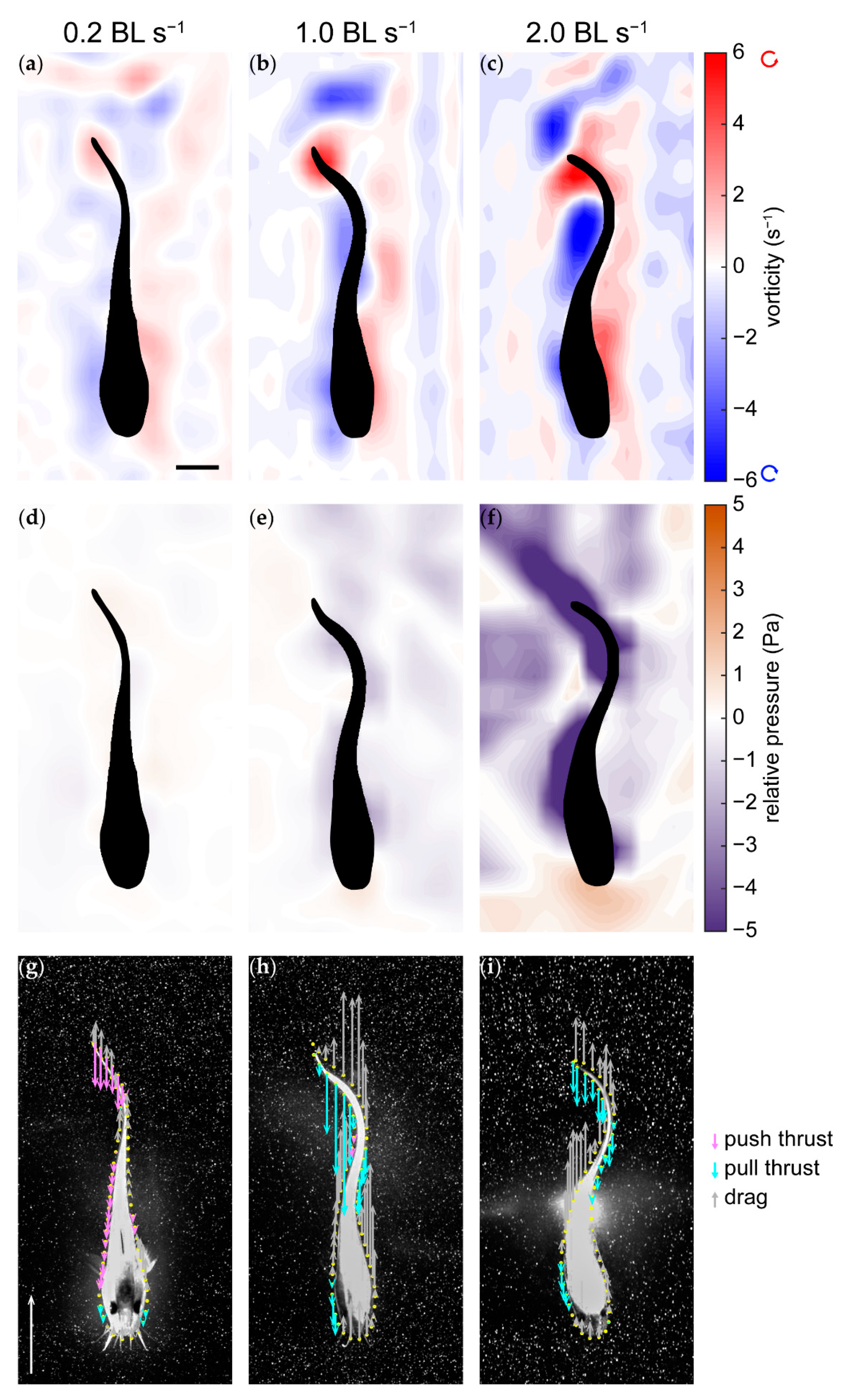
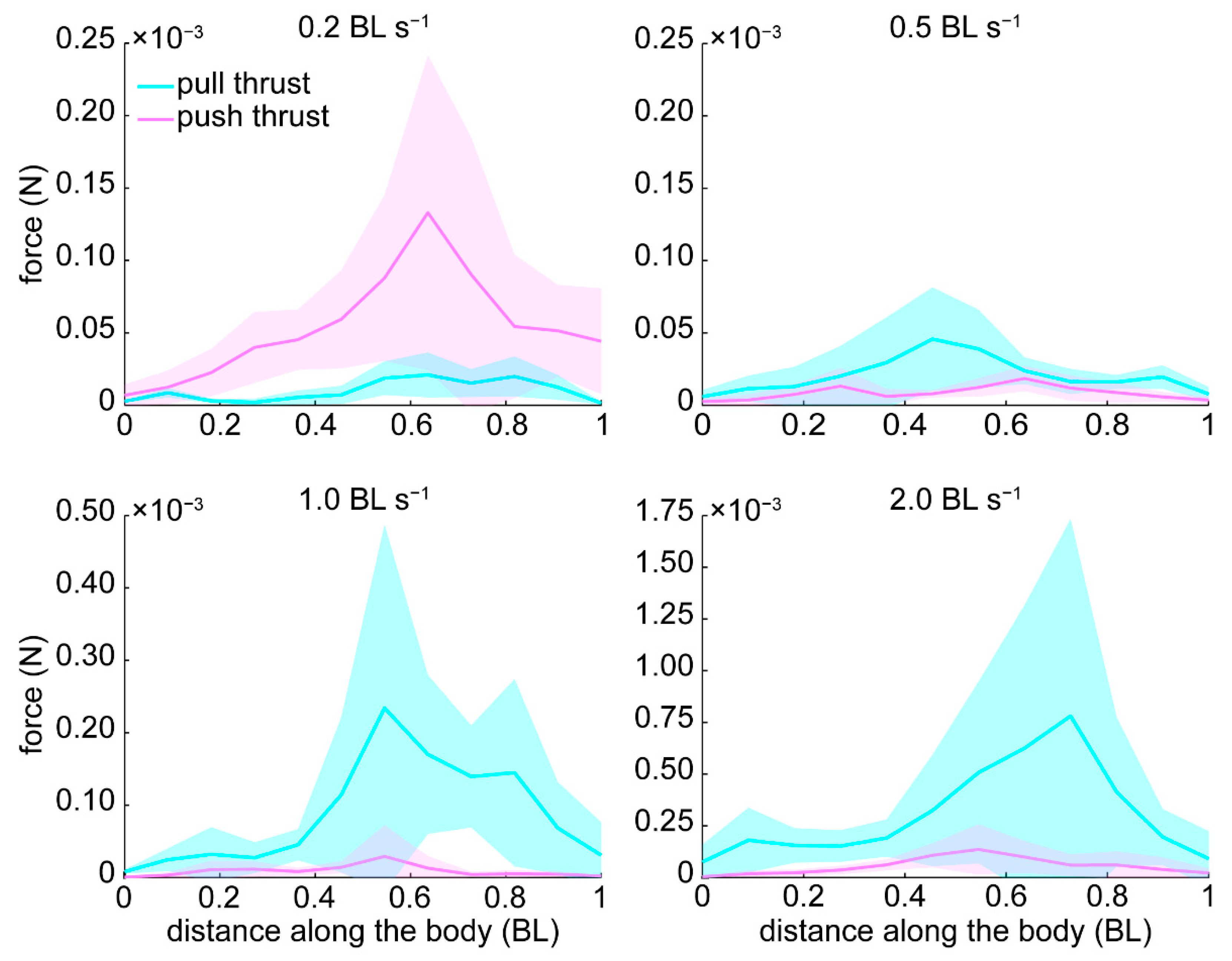
3.3. Pressure and Forces

Forces applied at the body—fluid interface were calculated based on a normalized depth profile of the fish (Figure S1) and were differentiated as push and pull forces based on the contribution of above-ambient (positive) and sub-ambient (negative) pressures generating thrust forces along the x-axis (direction of swimming) and drag forces in the opposite direction.

At swimming speeds ≥1.0 BL s⁻¹, pressure fields were dominated by strong negative pressures within the trough of a body wave that resulted from the production of proto-vortices due to the local rotation of the body surface as a body wave traveled posteriorly (Figure 5b,c,e,f). These pressure fields corresponded to strong pull forces (Figure 5h,i). The significance of pull forces in thrust production during steady swimming has been previously demonstrated [17,18]. However, at 0.2 BL s⁻¹, the lack of pronounced body bending anteriorly to the tip of the tail did not allow for the formation and circulation of proto-vortices capable of generating low-pressure areas near the body (Figure 5a–d). This resulted in the production of push rather than pull thrust through reactive forces (Figure 5g).

The push to pull ratio of the forces contributing to thrust varied significantly from 5.38 ± 0.41 to 0.53 ± 0.33 (p < 0.001) between swimming speeds of 0.2 BL s⁻¹ and 0.5 BL s⁻¹ respectively, thus indicating a reversal of the contribution of these forces to thrust (Figure 6). For speeds ≥0.5 BL s⁻¹ this ratio was always less than 1. This was indicative of push-dominated thrust at 0.2 BL s⁻¹ and pull-dominated thrust at speeds ≥0.5 BL s⁻¹ (Figure 6). Additionally, the magnitude of both push and pull thrust increased with increasing swimming speed ≥0.5 BL s⁻¹ (Figure 6a). Note that at 0.2 BL s⁻¹, the total thrust produced is greater than at 0.5 and 1.0 BL s⁻¹ despite the lower swimming speed (Figure 6a). Here, total thrust does not account for the effects of out-of-plane drag produced by the abduction of the pectoral, pelvic, and first dorsal fins at speeds less than 0.5 BL s⁻¹.

The distribution and magnitude of the push and pull forces along the body also varied with swimming speed (Figure 5g–i and Figure 7). At the lowest swimming speed of 0.2 BL s⁻¹, push thrust was dominant over pull thrust and was primarily generated in the posterior section of the body, reaching a peak at 0.63 BL along the length of the fish. Conversely, at higher speeds (≥0.5 BL s⁻¹), pull thrust was dominant (Figure 6 and Figure 7). In all cases, the combination of the shape of the body (Figure S1) with body kinematics (Figure 4) resulted in peak thrust of increasing magnitude with swimming speed located anteriorly to the tip of the tail (Figure 7). The location along the body at which pull thrust peaked moved slightly posteriorly with increasing swimming speed, from approximately 0.45 BL to 0.75 BL for speeds of 0.5 BL s⁻¹ to 2.0 BL s⁻¹ respectively.

4. Discussion

4.1. Energetics and Efficiency

Anguilliform locomotion has been associated with high energetic efficiency [1,20,30]. Recent studies have suggested that sub-ambient pressure dominated pull thrust may be one of the reasons for such efficient locomotion [17,18,21]. However, we do not currently understand how this mechanism changes over a range of natural swimming speeds. This is important as fish vary swimming speeds regularly in nature and spend significant periods of time moving at speeds outside of their optimal swimming speed [31].

In general, the greatest energy expenditure is predicted to occur at the lowest and highest sustainable speeds while the minimum expenditure is achieved at intermediate speeds [32]. The basis of this theory is that controlling stability at the lowest speeds is more difficult, thus causing instability costs to increase with decreasing speed [33]. In contrast, at higher swimming speeds where inertial forces dominate (Re > 1000), energy expenditure is dictated by body drag, which is a function of velocity squared [34]. Consequently, there should be a range of intermediate swimming speeds at which fish swim relatively economically. Considered together, these distinct hydrodynamic forces acting on the fish during locomotion resulted in the J-shaped trend in the COT. This pattern is commonly seen in other fishes for which an initial sharp decline in the COT with increasing velocity occurs [35]. In our study, this corresponded to a 60% decrease in the COT between 0.14 and 0.5 BL s⁻¹ (Figure 2). At the lowest velocities where Re was indicative of a near-transitional flow regime, the catfish abducted their pectoral, first dorsal, and pelvic fins to enhance stability. The influence of viscous forces on the system was more apparent and likely created additional energy costs to counteract induced drag and postural instabilities [36].

The COT observed for coral catfish falls within the 1 to 8 J m⁻¹ kg⁻¹ range previously reported for many species [37]. However, this contrasts with the energy efficient Silver eel that can achieve a COT as low as 0.6 J m⁻¹ kg⁻¹ at its optimum swimming speed of 0.8 BL s⁻¹ [2,3,38]. This discrepancy may arise from physio-morphological differences such as body size and weight [39], with the smaller individuals consuming on average more energy per unit mass [37]. This is supported in part by the routine metabolic rate that we measured for coral catfish (see Figure S4) that was over twice that of eels that were up to 8 times longer and over 500 times heavier [2].

Despite the high routine metabolic demand, coral catfish are not inherently inefficient swimmers. When examining the motion of the body alone, the Strouhal number and the slip ratio can serve as simplified indices of propulsive efficiency as they offer useful insights about the amount of useful work produced by body undulations. Both measures indicated that coral catfish swam with greater efficiency at higher swimming speeds. Mechanical models of pitching and heaving airfoils have demonstrated that propulsive efficiency peaks within the narrow interval 0.2 < St < 0.4 [40,41]. During cruising, many animals maintain St near this optimal range [42,43], including the American eel [44], hagfish [22], and coral catfish swimming at the fastest swimming speed (Table 1). Such St have been shown to permit the maintenance of a well-defined series of vortices [45,46] along the body at speeds ≥1.0 BL s⁻¹ in this study (Figure 5). However, a St as high as 1.88 at 0.2 BL s⁻¹ is indicative of the far lower efficiency of the reduced body undulations (Figure 3b and Figure 4) when generating thrust and corresponds to an overall high COT. The reduced efficiency at speeds less than 0.5 BL s⁻¹ has been reported for other eel-like fish such as the Pacific and Atlantic hagfish [22]. Likewise, the slip ratio indicates a lower propulsive efficiency of the body waves at lower speeds (Table 1). A slip ratio closer to 1 indicates high mechanical efficiency of the propulsive body waves due to the minimization of the energy lost to lateral motion [5,47], thus mitigating power requirements [48]. Most anguilliform and elongate swimmers studied to date display relatively high slip values when swimming at speeds nearing 1.0 to 1.5 BL s⁻¹ [20,22,44,49,50,51]. Here, such increase in propulsive performance with swimming speed coincided with an overall decrease in the COT. This strong association seen in several species supports the idea that, in addition to physio-morphological requirements, the performance of anguilliform swimming is mediated by hydromechanical factors.

4.2. Speed-Dependent Kinematics and Near-Body Vorticity

Anguilliform swimmers are known to alter body kinematics with swimming speed [4,20,44,51]. However, data currently exist for only a narrow range of naturally achievable swimming speeds. In addition, because of the difficulty to separate thrust and drag and their resulting effects when experimentally measuring the wake shed downstream [20,52,53,54,55], the hydrodynamic effects of variable body kinematics across speeds remain largely unquantified. Detailed body-fluid measurements over a range of natural swimming speeds enable us to quantify how the gradual development of important body—fluid interactions relate to efficient thrust generation. The body kinematics of coral catfish was comparable to that of the traditional exemplars of anguilliform locomotion including eels (Anguilla sp.) [20,51,56] and sea lampreys (Petromyzon marinus) [6,21,57]. Body waves were initiated just posteriorly to the head and travelled rearward with increasing wave amplitude (Figure 4). Tail-beat frequency also showed a strong positive linear association with relative swimming speed analogous to that of eels [44,51] and hagfish [22]. This relationship persisted across the full range of natural speeds spanning two orders of magnitude (Figure 3a). Altering undulation frequency alone can explain the proportional change in swimming speeds, but body waveform characteristics can also serve in modulating speed [44,58]. The shape of the amplitude envelopes obtained from centerline profiles showed a striking increase in the amplitude envelope area (total lateral displacement of the body) with speed (Figure 4). Such variation was caused by (1) the increase in the rate of growth of the amplitude of traveling body waves with speed, and (2) the greater involvement of anterior sections of the body. The resulting kinematics produced amplitude envelopes with concave outer bounds at speeds ≤0.5 BL s⁻¹. Although little data exist for such speeds, eels [44,49,51] and hagfish [22] swimming at 0.5 BL s⁻¹ tend to display comparable amplitude envelopes that are narrow along most of the body but wider in the last 20% of the length of the body. This pattern is generally observed in carangiform and thunniform species whose body undulations are confined to the caudal fin which acts as the main propeller [59,60]. However, contrary to other body-caudal fin swimming modes, the magnitude of the lateral displacement at the tip of the tail did not vary with swimming speed. Instead, changes in the total area of displacement of the body with swimming speed were primarily caused by the three-fold increase in the amplitude of sections of the body located between 0.4 and 0.8 BL. This suggests an increasing contribution of the mid-body for thrust generation at higher swimming speeds.

How does recruiting more anterior portions of the body impact the resulting fluid dynamics? Coordinated body movements are paramount to producing and organizing vorticity along the body to generate thrust efficiently [17,18,19,20,21]. Coral catfish are a good model for examining body—fluid interactions because their thrust is dominated by inertial rather than viscous forces (Re > 1000), and they build vorticity along their bodies gradually. As swimming speed increased and travelling waves began more anteriorly, we found a clear speed-dependent effect on the magnitude and distribution of vorticial structures along the body. The steady increase in body amplitude at higher swimming speeds led to increasing lateral displacement of the entire body that served in continually building fluid vorticity (Figure 3, Figure 4 and Figure 5b,c). Eels and lampreys swimming at their respective preferred relative speeds of 1.0 BL s⁻¹ [19] and 1.5 to 2.0 BL s⁻¹ [21] display comparable vorticity fields. In contrast, at 0.2 BL s⁻¹, peak vorticity during one complete tail beat was located at the very tip of the tail where body movements were concentrated. The importance of modulating body wave amplitude along the entirety of the body for vorticity control was evident in how effectively the catfish maintained greater propulsive efficiency with increasing swimming speed. Because the development of important interactions at the fluid-animal interface shows a dependence on body kinematics due to swimming speed, the nature of the forces generated is also expected to vary considerably.

4.3. Pressure and Thrust Resulting from Varying Hydrodynamic Conditions

Experimentally derived pressure fields around swimming fish enable us to identify the nature of the animal—fluid interactions driving efficient thrust production, and conversely, contributing to energy losses. In the inertial flow regime experience by the fish (Re > 1000), above-ambient pressure fields in the flow are indicative of reactive forces opposing the motion such as at the head, or during lateral body acceleration. In contrast, vortices and areas of accelerated velocities forming in the trough of a body wave are associated with regions of sub-ambient pressures [27,61]. To this date, little is known about the dynamics between sub-ambient pressure dominated pull and reactive push forces, particularly across a range of swimming speeds, Re, and body kinematics. Identifying the limitations of this relationship is necessary to discern the mechanisms driving energy-efficient anguilliform locomotion. Similar to experiments involving lampreys [17,18], the gradual development of areas of vorticity along the body gradually developed large sub-ambient pressure zones in the troughs of the traveling waves (Figure 5). The pull forces from these sub-ambient pressure regions not only increased in magnitude with speed, but their overall relative contribution to thrust also showed the same dependence to speed. The pull exerted by these regions largely surpassed the contribution of reactive forces and were the primary thrust mechanisms. This was more evident at 1.0 and 1.5 BL s⁻¹ where pull forces contributed to 87% of the total thrust (Figure 6). Our observation of how a considerable proportion of pull forces is acting on the body at these speeds were comparable to what has been described for lampreys [17,21]. This is interesting because, in these recent studies, the lampreys were swimming at their preferred swimming speed of about 1.5 BL s⁻¹. Anguilliform swimmers may naturally favor swimming speeds at which thrust is generated efficiently through dominant pull forces, especially since this mechanism is associated with a low COT. This substantial proportion of pull forces acting on the body is also strikingly representative of the best energetic performance attained by the well-documented American eel [2,3] swimming within the same range of speeds. Additionally, the relatively wide range of speeds (achievable by eel-like fish) at which pull forces dominate total thrust reveals the ubiquity of this propulsive mechanism among anguilliform species.

Past 2.0 BL s⁻¹, coral catfish could not maintain steady swimming and generally quit swimming entirely. Kinematics parameters indicate that the fish could increase both body wave amplitude and tail-beat frequency to enhance the strength of near-body sub-ambient pressure fields. Nevertheless, they could not perform reliably past this speed threshold. This limitation did not correspond to a decrease in the magnitude of both push and pull forces but instead coincided with the slight increase in the push:pull ratio. The production of faster body waves likely increased acceleration reactions that resisted the axial and lateral movement of the body [31]. The resulting reactive forces could contribute to greater losses in kinetic energy, thus incurring a cost on performance and limiting the fish’s ability to swim faster. However, such added energy cost was not captured though respirometry. Can we even expect a reversal of the ratio of push to pull forces past 2.0 BL s⁻¹? The limits imposed by a biological model may not be able to answer this question. However, a reversal in this ratio was observed between 0.2 and 0.5 BL s⁻¹ where propulsion was achieved without the build-up of strong vortices along the body (Figure 6). In contrast to the other speeds tested, at 0.2 BL s⁻¹, the fish relied largely on positive pressure fields acting on the posterior third of the body where push thrust accounted for about 85% of the total thrust (Figure 7). This is a direct consequence of the limited lateral motion of the body that did not allow for the production and circulation of the same sub-ambient pressure fields that we observed at the higher speeds. The reversal in the contribution of push and pull forces to total thrust was associated with a sharp decline in the COT by nearly 60%. This change in the nature of the thrust produced highlights the overall energy-efficient properties of pull-dominated thrust.

Regardless of whether thrust was push- or pull-dominated, peak total thrust was produced along the posterior half of the body, where changes in the lateral displacement of the body showed the most variation across swimming speeds (Figure 7). Similar to lampreys, most of the useful thrust was generated along the rear half of the body [18,21]. Thrust did not peak at the tip of the tail, however. This seemingly counterintuitive result can be explained by two factors: (1) the body depth profile of the fish showed a visible taper at the tip of the tail (Figure S1), thus decreasing the surface area available to generate thrust; (2) the amplitude of the tip of the tail did not vary significantly across speeds. While the lateral excursions of most of the body is modulated by both tail-beat frequency and amplitude, the motion of the extremity of the tail is primarily dictated by tail-beat frequency only. Thus, the limited ability to control the motion of the tail at this location renders this section of the body less favorable to modulate thrust production. Interestingly, we also found that on average, at 0.2 BL s⁻¹, the magnitude of the total thrust generated was greater than that produced at 0.5 BL s⁻¹ (Figure 6a). At this swimming speed, the fish abducted their pectoral, first dorsal, and pelvic fins most likely to enhance stability [36,62]. Swimming at a Re near the transitional regime will render the influence of viscous forces on the system more apparent (Table 1). The drag produced by all these surfaces could not be quantified here due to the two-dimensional nature of the velocity fields acquired experimentally. Nonetheless, this certainly resulted in additional friction and form drag that the fish had to compensate for to maintain steady swimming [36].

5. Conclusions

The investigation of energetics, swimming kinematics, pressure fields, and force components of Plotosus lineatus swimming over a range of natural swimming speeds demonstrated that energy-efficient pull thrust served as a primary propulsive mechanism. However, low swimming speeds did not allow for sufficient body bending to generate the strong upstream vortices required for sub-ambient pressures to form near the body. Thus, this corresponded to an overall higher COT. A recurrent limitation that we also found in our study is the overall inability of the majority of eel-like swimmers studied to date, including various taxa, to maintain steady swimming past 2.0 BL s⁻¹ [2,3,22,44,51]. Because of this, we still lack an understanding of the recruitment of the pull and reactive push forces at speeds that are otherwise commonly achieved with the carangiform and the thunniform modes of swimming. Does the increase found in the upper bound of swimming speeds for other species’ “J shaped” COT curve correspond to a relative reduction in the sub-ambient pressure driven pull thrust? Live fish may not be able to provide an answer to this question. Thus, novel approaches in the study of fish locomotion using robotic devices, mechanical models, and computational fluid dynamics [63,64,65,66] may shed additional light on the limiting factors of eel-like locomotion beyond the maximum speed obtained experimentally with biological models.

References

1. van Ginneken, V.; Antonissen, E.; Müller, U.K.; Booms, R.; Eding, E.; Verreth, J.; van den Thillart, G. Eel migration to the Sargasso: Remarkably high swimming efficiency and low energy costs. J. Exp. Biol. 2005, 208, 1329–1335. [Google Scholar] [CrossRef] [Green Version]
2. van den Thillart, G.; Palstra, A.; van Ginneken, V. Simulated migration of European silver eel; swim capacity and cost of transport. J. Mar. Sci. Technol. 2007, 15, 1–16. [Google Scholar]
3. Palstra, A.; van Ginneken, V.; van den Thillart, G. Cost of transport and optimal swimming speed in farmed and wild European silver eels (Anguilla anguilla). Comp. Biochem. Phys. A 2008, 151, 37–44. [Google Scholar] [CrossRef] [PubMed]
4. Gray, J. Studies in animal locomotion: II. The relationship between waves of muscular contraction and the propulsive mechanism of the eel. J. Exp. Biol. 1933, 10, 88–104. [Google Scholar]
5. Sigvardt, K.A. Spinal mechanisms in the control of lamprey swimming. Am. Zool. 1989, 29, 19–35. [Google Scholar] [CrossRef]
6. Williams, T.L.; Grillner, S.; Smoljaninov, V.V.; Wallén, P.; Kashin, S.; Rossignol, S. Locomotion in lamprey and trout: The relative timing of activation and movement. J. Exp. Biol. 1989, 143, 559–566. [Google Scholar]
7. Wardle, C.; Videler, J.; Altringham, J. Tuning in to fish swimming waves: Body form, swimming mode and muscle function. J. Exp. Biol. 1995, 198, 1629–1636. [Google Scholar]
8. Warren, C.E.; Davis, G.E. Laboratory studies on the feeding, bioenergetics, and growth of fish. Or. State Univ. Agric. Exp. Station Spec. Rep. 1967, 230, 175–214. [Google Scholar]
9. Steffensen, J.F.; Johansen, K.; Bushnell, P.G. An automated swimming respirometer. Comp. Biochem. Phys. A. 1984, 79, 437–440. [Google Scholar] [CrossRef]
10. Brett, J.R.; Groves, T.D.D. Physiological energetics. Fish Physiol. 1979, 8, 280–352. [Google Scholar]
11. Noca, F.; Shiels, D.; Jeon, D. Measuring instantaneous fluid dynamic forces on bodies, using only velocity fields and their derivatives. J. Fluid Struct. 1997, 11, 345–350. [Google Scholar] [CrossRef]
12. Gurka, R.; Liberzon, A.; Hefetz, D.; Rubinstein, D.; Shavit, U. Computation of pressure distribution using piv velocity data. In Proceedings of the 3rd International Workshop on Particle Image Velocimetry, Santa Barbara, CA, USA, 16 September 1999; Adrian, R., Ed.; Springer: Berlin/Heidelberg, Germany, 1999. [Google Scholar]
13. Lauder, G.V.; Tytell, E.D. Hydrodynamics of undulatory propulsion. Fish Physiol. 2005, 23, 425–468. [Google Scholar]
14. van Oudheusden, B.W.; Scarano, F.; Roosenboom, E.W.M.; Casimiri, E.W.F.; Souverein, L.J. Evaluation of integral forces and pressure fields from planar velocimetry data for incompressible and compressible flows. Exp. Fluids 2007, 43, 153–162. [Google Scholar] [CrossRef] [Green Version]
15. Dabiri, J.O.; Bose, S.; Gemmell, B.J.; Colin, S.P.; Costello, J.H. An algorithm to estimate unsteady and quasi-steady pressure fields from velocity field measurements. J. Exp. Biol. 2014, 217, 331–336. [Google Scholar] [CrossRef] [Green Version]
16. Lucas, K.N.; Dabiri, J.O.; Lauder, G.V. A pressure-based force and torque prediction technique for the study of fish-like swimming. PLoS ONE 2017, 12, e0189225. [Google Scholar] [CrossRef] [Green Version]
17. Gemmell, B.J.; Colin, S.P.; Costello, J.H.; Dabiri, J.O. Suction-based propulsion as a basis for efficient animal swimming. Nat. Commun. 2015, 6, 8790. [Google Scholar] [CrossRef] [PubMed] [Green Version]
18. Gemmell, B.J.; Fogerson, S.M.; Costello, J.H.; Morgan, J.R.; Dabiri, J.O.; Colin, S.P. How the bending kinematics of swimming lampreys build negative pressure fields for suction thrust. J. Exp. Biol. 2016, 219, 3884–3895. [Google Scholar] [CrossRef] [Green Version]
19. Müller, U.K.; Smit, J.; Stamhuis, E.; Videler, J. How the body contributes to the wake in undulatory fish swimming: Flow fields of a swimming eel (Anguilla anguilla). J. Exp. Biol. 2001, 204, 2751–2762. [Google Scholar]
20. Tytell, E.D.; Lauder, G.V. The hydrodynamics of eel swimming: I. Wake structure. J. Exp. Biol. 2004, 207, 1825–1841. [Google Scholar] [CrossRef] [PubMed] [Green Version]
21. Clos, K.T.D.; Dabiri, J.O.; Costello, J.H.; Colin, S.P.; Morgan, J.R.; Fogerson, S.M.; Gemmell, B.J. Thrust generation during steady swimming and acceleration from rest in anguilliform swimmers. J. Exp. Biol. 2019, 222, jeb212464. [Google Scholar] [CrossRef]
22. Lim, J.L.; Winegard, T.M. Diverse anguilliform swimming kinematics in Pacific hagfish (Eptatretus stoutii) and Atlantic hagfish (Myxine glutinosa). Can. J. Zool. 2015, 93, 213–223. [Google Scholar] [CrossRef]
23. Svendsen, M.B.S.; Bushnell, P.G.; Steffensen, J.F. Design and setup of intermittent-flow respirometry system for aquatic organisms. J. Fish Biol. 2016, 88, 26–50. [Google Scholar] [CrossRef] [Green Version]
24. Elliott, J.M.; Davison, W. Energy equivalents of oxygen consumption in animal energetics. Oecologia 1975, 19, 195–201. [Google Scholar] [CrossRef]
25. Flammang, B.E.; Lauder, G.V.; Troolin, D.R.; Strand, T. Volumetric imaging of shark tail hydrodynamics reveals a three-dimensional dual-ring vortex wake structure. Proc. R. Soc. B Biol. Sci. 2011, 278, 3670–3678. [Google Scholar] [CrossRef] [PubMed] [Green Version]
26. Gemmell, B.J.; Adhikari, D.; Longmire, E.K. Volumetric quantification of fluid flow reveals fish’s use of hydrodynamic stealth to capture evasive prey. J. R. Soc. Interface 2014, 11, 20130880. [Google Scholar] [CrossRef] [PubMed] [Green Version]
27. Batchelor, G.K. An Introduction to Fluid Mechanics; Cambridge University Press: Cambridge, UK, 1973. [Google Scholar]
28. Wang, J.; Zhang, C.; Katz, J. GPU-based, parallel-line, omni-directional integration of measured pressure gradient field to obtain the 3D pressure distribution. Exp. Fluids 2019, 60, 58. [Google Scholar] [CrossRef]
29. Zar, J.H. Biostatistical Analysis, 4th ed.; Pearson: Bergen, NJ, USA, 1999; pp. 35–424. [Google Scholar]
30. William, F.; Beamish, H. Migration and spawning energetics of the anadromous sea lamprey, Petromyzon marinus. Environ. Biol. Fishes 1979, 4, 3–7. [Google Scholar] [CrossRef]
31. Daniel, T.L. Unsteady aspects of aquatic locomotion. Am. Zool. 1984, 24, 121–134. [Google Scholar] [CrossRef] [Green Version]
32. Di Santo, V.; Kenaley, C.P.; Lauder, G.V. High postural costs and anaerobic metabolism during swimming support the hypothesis of a U-shaped metabolism-speed curve in fishes. Proc. Natl. Acad. Sci. USA 2017, 114, 13048–13053. [Google Scholar] [CrossRef] [Green Version]
33. Webb, P.W. Control of posture, depth, and swimming trajectories of fishes. Integr. Comp. Biol. 2002, 42, 94–101. [Google Scholar] [CrossRef]
34. Di Santo, V.; Blevins, E.L.; Lauder, G.V. Batoid locomotion: Effects of speed on pectoral fin deformation in the little skate, Leucoraja erinacea. J. Exp. Biol. 2017, 220, 705–712. [Google Scholar] [CrossRef] [PubMed] [Green Version]
35. Kendall, J.L.; Lucey, K.S.; Jones, E.A.; Wang, J.; Ellerby, D.J. Mechanical and energetic factors underlying gait transitions in bluegill sunfish (Lepomis macrochirus). J. Exp. Biol. 2007, 210, 4265–4271. [Google Scholar] [CrossRef] [Green Version]
36. Webb, P.W. Stability and maneuverability. Fish Physiol. 2005, 23, 281–332. [Google Scholar]
37. Schmidt-Nielsen, K. Locomotion: Energy cost of swimming, flying, and running. Science 1972, 177, 222–228. [Google Scholar] [CrossRef]
38. Palstra, A. Energetic Requirements and Environmental Constraints of Reproductive Migration and Maturation of European Silver Eel (Anguilla anguilla L.). Ph.D. Thesis, University of Leiden, Leiden, The Netherlands, 2006. [Google Scholar]
39. Goolish, E.M. The metabolic consequences of body size. In Biochemistry and Molecular Biology of Fishes; Hochachka, P.W., Mommsen, T.P., Eds.; Elsevier: Amsterdam, The Netherlands, 1995; Volume 4, pp. 335–366. [Google Scholar]
40. Triantafyllou, G.S.; Triantafyllou, M.S.; Grosenbauch, M.A. Optimal thrust development in oscillating foils with application to fish propulsion. J. Fluids Struct. 1993, 7, 205–224. [Google Scholar] [CrossRef]
41. Triantafyllou, M.S.; Triantafyllou, G.S. An efficient swimming machine. Sci. Am. 1995, 272, 40–46. [Google Scholar] [CrossRef]
42. Taylor, G.K.; Nudds, R.L.; Thomas, A.L.R. Flying and swimming animals cruise at a Strouhal number tuned for high power efficiency. Nature 2003, 425, 707–711. [Google Scholar] [CrossRef] [PubMed]
43. Eloy, C. Optimal Strouhal number for swimming animals. J. Fluids Struct. 2012, 30, 205–218. [Google Scholar] [CrossRef] [Green Version]
44. Tytell, E.D. The hydrodynamics of eel swimming II. Effect of swimming speed. J. Exp. Biol. 2004, 207, 3265–3279. [Google Scholar] [CrossRef] [Green Version]
45. Anderson, J.M.; Streitlien, K.; Barrett, D.S.; Triantafyllou, M.S. Oscillating foils of high propulsive efficiency. J. Fluid Mech. 1998, 360, 41–72. [Google Scholar] [CrossRef] [Green Version]
46. Wang, Z.J. Vortex shedding and frequency selection in flapping flight. J. Fluid Mech. 2000, 410, 323–341. [Google Scholar] [CrossRef] [Green Version]
47. Müller, U.K.; Stamhuis, E.J.; Videler, J.J. Riding the waves: The role of the body wave in undulatory fish swimming. Integr. Comp. Biol. 2002, 42, 981–987. [Google Scholar] [CrossRef]
48. Yu, C.L.; Hsu, Y.H.; Yang, J.T. The dependence of propulsive performance on the slip number in an undulatory swimming fish. Ocean Eng. 2013, 70, 51–60. [Google Scholar] [CrossRef]
49. Gillis, G. Undulatory locomotion in elongate aquatic vertebrates: Anguilliform swimming since Sir James Gray. Am. Zool. 1996, 36, 656–665. [Google Scholar] [CrossRef]
50. Gillis, G. Anguilliform locomotion in an elongate salamander (Siren intermedia): Effects of speed on axial undulatory movements. J. Exp. Biol. 1997, 200, 767–784. [Google Scholar]
51. D’Aout, K.; Aerts, P. A kinematic comparison of forward and backward swimming in the eel Anguilla anguilla. J. Exp. Biol. 1999, 202, 1511–1521. [Google Scholar]
52. Lighthill, M.J. Hydromechanics of aquatic animal propulsion. Annu. Rev. Fluid Mech. 1969, 1, 413–466. [Google Scholar] [CrossRef]
53. Lighthill, M.J. Large-amplitude elongated-body theory of fish locomotion. Proc. R. Soc. B Biol. Sci. 1971, 179, 125–138. [Google Scholar]
54. Weihs, D. The mechanisms of rapid starting of slender fish. Biorheology 1973, 10, 343–350. [Google Scholar] [CrossRef] [PubMed]
55. Weihs, D. Design features and mechanics of axial locomotion in fish. Am. Zool. 1989, 29, 151–160. [Google Scholar] [CrossRef]
56. Gillis, G.B. Environmental effects on undulatory locomotion in the American eel Anguilla rostrata: Kinematics in water and on land. J. Exp. Biol. 1998, 201, 949–961. [Google Scholar]
57. Williams, T.L.; Bowtell, G.; Carling, J.C.; Sigvardt, K.A.; Curtin, N.A. Interactions between muscle activation, body curvature and the water in the swimming lamprey. In Biological Fluid Dynamics; Ellington, C.P., Pedley, T.J., Eds.; The Company of Biologists Ltd.: Cambridge, UK, 1995; pp. 49–59. [Google Scholar]
58. Liao, J.C. Swimming in needlefish (Belonidae): Anguilliform locomotion with fins. J. Exp. Biol. 2002, 205, 2875–2884. [Google Scholar] [PubMed]
59. Webb, P.W. Form and function in fish swimming. Sci. Am. 1984, 251, 72–83. [Google Scholar] [CrossRef]
60. Müller, U.K.; van Leeuwen, J.L. Undulatory fish swimming: From muscles to flow. Fish Fish. 2006, 7, 84–103. [Google Scholar] [CrossRef]
61. Li, G.; Müller, U.K.; van Leeuwen, J.L.; Liu, H. Body dynamics and hydrodynamics of swimming fish larvae: A computational study. J. Exp. Biol. 2012, 215, 4015–4033. [Google Scholar] [CrossRef] [Green Version]
62. Sfakiotakis, M.; Lane, D.; Davies, J. Review of fish swimming modes for aquatic locomotion. IEEE J. Oceanic Eng. 1999, 24, 237–252. [Google Scholar] [CrossRef] [Green Version]
63. Lauder, G.V.; Drucker, E.G. Forces, fishes, and fluids: Hydrodynamic mechanisms of aquatic locomotion. News Physiol. Sci. 2002, 17, 235–240. [Google Scholar] [CrossRef] [Green Version]
64. Borazjani, I.; Sotiropoulos, F. On the role of form and kinematics on the hydrodynamics of self-propelled body/caudal fin swimming. J. Exp. Biol. 2010, 213, 89–107. [Google Scholar] [CrossRef] [PubMed] [Green Version]
65. Lauder, G.V.; Flammang, B.; Alben, S. Passive robotic models of propulsion by the bodies and caudal fins of fish. Integr. Comp. Biol. 2012, 52, 576–587. [Google Scholar] [CrossRef] [Green Version]
66. Wen, L.; Lauder, G. Understanding undulatory locomotion in fishes using an inertia-compensated flapping foil robotic device. Bioinspir. Biomim. 2013, 8, 046013. [Google Scholar] [CrossRef] [Green Version]
Figure 1. Modified Brett-type swim tunnel respirometer used for particle image velocimetry (PIV) and respirometry experiments (top view). PIV experiments were conducted without the optional flow-through respirometry loop (Ro and Ri closed) but included a high-speed camera mounted on top of the test section and pointing down. (A) Buffer tank, (B) swim tunnel respirometer, (1) motor, (2) impeller, (3) fin-type flow straightener, (4) back-flow dampener/disturbance plate (coarse filter), (5) flow straightener (vanes), (6) honey-comb flow straightener, (7) transparent acrylic wall, (8) metallic mesh, (9) plano-concave lens, (10) mirror.
Fluids 06 00127 g001
Figure 2. Cost of transport (COT). The metabolic cost of swimming at speeds (U) ranging from 0.14 to 2.0 BL s−1 decreased exponentially with swimming speed. The equation for the fitted line (solid red line) is COT = αeβU + γeδU, where α = 78.05 j m−1 kg−1, β = 3.39 s BL−1, γ = 9.79 j m−1 kg−1, δ = −0.20 s BL−1 (R2 = 0.69).
Fluids 06 00127 g002
Figure 3. Tail-beat frequency and amplitude envelope area. (a) Mean tail-beat frequency (f) measured at the tip of the tail shows a strong linear relationship with swimming speed (U) in the form of f = αU + β where α = 1.366 BL−1 and β = 1.509 s−1 (R2 = 0.997; r = 0.998; p < 0.01). (b) The relationship between mean amplitude envelope area A (normalized to BL2) and swimming speed is expressed as A = γU + δ where γ = 0.026 BL s and δ = 0.047 BL2 (R2 = 0.991; r = 0.995; p < 0.01). Error bars represent standard deviation.
Fluids 06 00127 g003
Figure 4. Kinematics and body—wave amplitude envelope at different swimming speeds. (ae) Stacked midlines corresponding to one complete tail beat are of one representative fish swimming steadily at swimming speeds of 2.0, 1.5, 1.0, 0.5, and 0.2 BL s−1. Although the fish were swimming steadily, the centerlines were fixed at the same origin on the x-axis (coincident to the direction of swimming) for each tail beat. The centerlines were traced every 0.04 s (every 20 frames). (f) Means ± s.d. lateral displacement of 6 points equally distributed along the midline of the fish for each swimming speed over one complete tail beat.
Fluids 06 00127 g004
Figure 5. Vorticity, pressure, and force components. Selected frames during steady swimming at 0.2, 1.0, and 2.0 BL s−1. (ac) vorticity fields with velocity vectors. The scale arrow indicates 0.5 m s−1. (df) Pressure fields. (gi) Thrust and drag component vectors. The scale arrow indicates 0.01 N m−1. The scale bars indicate 10 mm for all frames.
Fluids 06 00127 g005
Figure 6. Contribution of push and pull forces to total thrust. (a) Boxplot diagram showing the magnitude of pull and push thrust forces for speeds ranging from 0.2 to 2.0 BL s−1. For each component of thrust, means identified by the same-colored letters are not significantly different (p > 0.05). (b) Boxplot diagram showing the relative contribution of push and pull forces to thrust. A ratio greater than 0 indicates that thrust is primarily generated through push forces while a ratio less than 0 indicates that pull thrust is dominant.
Fluids 06 00127 g006
Figure 7. Distribution of push and pull forces along the body during one tail-beat cycle. Mean thrust components plotted against normalized body length (BL) for swimming speeds of 0.2 BL s−1, 0.5 BL s−1, 1.0 BL s−1, and 2.0 BL s−1. Shading indicates standard deviation.
Fluids 06 00127 g007