Article

A Comparison of Ansys Fluent and MFiX in Performing CFD-DEM Simulations of a Spouted Bed

Department of Civil, Chemical and Environmental Engineering (DICCA), University of Genova, 16145 Genova, Italy
*
Author to whom correspondence should be addressed.
Fluids 2021, 6(11), 382; https://doi.org/10.3390/fluids6110382
Submission received: 28 September 2021 / Revised: 19 October 2021 / Accepted: 20 October 2021 / Published: 25 October 2021

Abstract

:
The CFD-DEM methodology is a popular tool for the study of fluid–particle systems, and there are several programs that permit using it. In this study, we employed it to simulate a pseudo-2D spouted bed, comparing the performance of the programs Ansys Fluent and MFiX. The results are analysed and commented on in terms of both accuracy and computational efforts. Despite the similarity of the setup, MFiX seems to perform significantly better. The similarities and differences between the two programs are discussed in detail, offering useful insights to researchers regarding the selection of one over the other, depending on the application. The better suitability of the Di Felice drag model is confirmed for the device, while it is shown that the effect of the Magnus lift force may be more limited than was shown in a previous study.

1. Introduction

Complex numerical simulations have seen an intense growth in the last two decades, thanks to the release of better-performing and widely accessible computational resources. Even without expensive supercomputers, researchers can provide meaningful contributions in areas with notable open questions, such as turbulence, molecular dynamics, climate science, etc. Among these, the behaviour of granular materials is a very popular research field. Despite the numerous efforts of researchers, a deep understanding of many features of these flows is still lacking [1]. Several numerical techniques have been developed to reproduce the behaviour of granular flows at various scales, from the very detailed but complex direct numerical simulations to lighter methods based on the continuum hypothesis [2,3]. In this framework, the combination of computational fluid dynamics (CFD) and the discrete element method (DEM), widely known as CFD-DEM, represents a good compromise between computational complexity and accuracy [4].
CFD-DEM, which is a Eulerian–Lagrangian approach, simulates particles according to the discrete element method, originally proposed in 1979 by Cundall and Strack [5]. The method treats each physical particle (or group of particles) as a computational particle, with the collisions among them directly resolved. DEM was first coupled with CFD in 1992 thanks to the work of Tsuji and colleagues [6], thus allowing the simulation of multiphase flows. CFD-DEM represents a suitable option when the number of particles is not excessive and is generally deemed as more reliable than continuum methods, also providing more detailed results [7,8,9]. One of its drawbacks is that the computational grid must be larger than the particles, thus possibly leading to inaccuracies in predicting the behaviour of the fluid phase [10]. Due to this requirement, the method is labelled as “unresolved”. The interaction between the fluid and solid phase(s) relies on models that estimate the drag force based on experimental or numerical techniques. Several models exist in the literature, but researchers disagree on the ideal choice, and none of them appear to be suitable in all operative conditions [11].
CFD-DEM has become particularly common in the last decade. According to the Scopus database (www.scopus.com, accessed on 18 October 2021), the first scientific article that features the expression “CFD-DEM” in its title, abstract, or keywords dates back to 2003 [12]; 70 articles featured it (or a variation) in 2013, 125 in 2016, and 292 in 2020. This growth is directly ascribable not only to the enhancement of computational resources, but also to the release of several accessible programs. These allowed researchers to perform such simulations without having to develop a whole in-house code, on which research works were originally (and sometimes still are) based.
Programs can be categorised as open-source or commercial. Open-source programs have some clear advantages, such as being free and completely editable and transparent to the user, thus allowing more flexibility. However, the process of learning to use them at their full potential can be cumbersome, as sometimes they do not have a GUI (graphical user interface), require good coding skills and have limited support and tutorials [13]. On the other hand, commercial programs are usually not free, and their code is not completely visible or editable, but they may have more in-built features and better support resources. Commercial programs include Rocky and EDEM, whereas open-source programs include LIGGGHTS and Yade, among others.
This work focuses on two well-known programs that permit performing CFD-DEM simulations: MFiX and Ansys Fluent. MFiX (Multiphase Flow with interphase eXchanges, mfix.netl.doe.gov, accessed on 18 October 2021) is an open-source program developed by the National Energy Technology Laboratory (NETL), part of the Department of Energy of the USA, which allows simulating granular materials through different methodologies. Conversely, Ansys Fluent (www.ansys.com/products/fluids/ansys-fluent, accessed on 18 October 2021) is a commercial program that allows performing a wide variety of CFD simulations. It is part of the Ansys package, which includes numerous other programs. Fluent can also be employed to perform the CFD calculations only, with the DEM ones being solved by a coupled commercial program (such as the aforementioned Rocky and EDEM). Despite their different licence, MFiX and Fluent can be considered among the most accessible programs for someone who wants to start performing CFD-DEM simulations: they both have a user-friendly GUI and are available for early-stage researchers either as an open-source program (MFiX), or through the student licence (Fluent). For this reason, they were chosen for the present analysis.
The two programs are compared for CFD-DEM simulations, focusing on the similarities and differences in preparing and personalising the simulation setup and in their accuracy and efficiency. The comparison is based on experimental data of a pseudo-2D spouted bed [14]. Spouted beds are a particular kind of fluidised beds, particularly suitable to be studied through CFD-DEM simulations as they typically work with relatively large Geldart-D [15] particles. Moreover, there are some open research questions regarding their fluid dynamic regime, despite the great number of studies focusing on these devices, including through CFD-DEM simulations as detailed in [16].
To the best of our knowledge, there is no existing study comparing CFD-DEM simulations performed with different codes, whereas for the Eulerian–Eulerian approach, Herzog et al. [17] compared MFiX, OpenFoam and Fluent, and Venier et al. [18] compared OpenFoam and Fluent, in both cases taking fluidised beds into account. The first study (published in 2012) concluded that MFiX and Fluent were almost equivalently accurate, with OpenFoam deemed as not mature enough yet. Conversely, the second study (published in 2019), stated that the two programs are almost equivalent in their accuracy, pointing out that both still have notable room for improvement.

2. Materials and Methods

2.1. Governing Equations

The simulation approach is based on the combination of CFD and DEM. The equations of the two methodologies, including their implementation in Fluent and MFiX, have been reported multiple times in the literature, and for the sake of conciseness they are not fully repeated here. Interested readers are referred to previous publications [19,20] or the official guides of the two programs [21,22,23]. This section discusses the main similarities and differences in the implementation of the methods.
Regarding the CFD part, both programs employ the equations of local balance for mass and momentum for the fluid phase. Fluent employs the so-called “model A”, whereas MFiX allows choosing between A and B [24]. In this work, model A was employed in both programs. The programs also offer the possibility of turning off the fluid solver and performing pure DEM simulations. However, in that case, Fluent’s performance is dubious [25], which is expected since its original aim is to perform fluid dynamics studies.
Coherently with its versatility, Fluent offers a wide variety of models to consider turbulence. Conversely, MFiX only has two turbulence models in its code (the k-epsilon and the L-scale models). Here, the k-epsilon model [26] was selected. Despite the fact it complicates the computational setup and is sometimes neglected when simulating spouted beds [16], turbulence can have an impact on CFD-DEM simulations [27] and it should be included for the sake of accuracy.
Regarding the DEM part, both programs solve the Newtonian equations of motion for all particles. While MFiX automatically solves both the translational and rotational equations, in Fluent the rotational equation has to be explicitly activated by the user. There are also some differences regarding the calculation of some forces that the particles experience. These are detailed below.

2.1.1. Pressure Gradient Force

Particles can perceive an acceleration caused by the fluid phase pressure gradient. This is usually quite small compared to other forces, especially when the fluid phase is gaseous. In Fluent, the force Fpg is given as:
F p g = m p ρ f ρ p u p u
In which mp is the particle mass, ρf and ρp are the fluid and particle density, and up and u are the particle and fluid velocity. In this equation, the pressure gradient is replaced by the velocity gradient based on a steady-state approach of the momentum equation, neglecting diffusive and source terms.
In MFiX, the force is instead calculated as:
F p g = V p , i P
in which Vp is the particle volume and P is the fluid pressure.

2.1.2. Drag Force

Both programs offer the possibility of choosing among several models to calculate the fluid–solid momentum exchange. Moreover, further models can be implemented through user-defined functions (UDF). These must be written in the C language for Fluent and in FORTRAN for MFiX. More information on implementing UDF drag models in Fluent is provided in a previous article [11]. In this work, we considered the Gidaspow [28] and Di Felice [29] drag models. For the Gidaspow model the force is thus calculated in Fluent:
F d = m p μ ρ p d p 2 ( u u p ) D
R e p = ε f ρ f d p | u p u | μ f
D = { 18   ε f 3.65 ( 1 + 0.15 ( R e p ) 0.687 )                                       f o r   ε s 0.2 150 ε s ε f 2 + 1.75 R e p ε f 2                                                                                         f o r   ε s > 0.2
In MFiX, the force is calculated as:
F d , i = β i V p , i ε s ( u u p )
β i = { 150 ( 1 ε f ) μ f ε f d p 2 + 1.75 ρ f | u u p | d p           i f   ε f 0.8 0.75 C D | u u p | ε f ρ f ε f 2.65 d i                             i f   ε f > 0.8
C D = { 24 R e p ( 1 + 0.15 R e p 0.687 )           i f   R e p < 1000 0.44                                                                         i f   R e p 1000
The procedure is analogous for the Di Felice drag model, with equations for D and βi that are as follows:
D = 0.75 C D R e p ε f 1 χ
β i = 0.75 C D | u u p | ρ f ε f 2 χ / d p
χ = 3.7 0.65 exp ( 0.5 ( 1.5 log 10 R e ) 2 )
in which CD is calculated as per Equation (8). In the above equations, μ is the fluid viscosity, dp the particle diameter, εf and εs the fluid and solid volume fraction.
The Gidaspow drag model is actually a mere combination of the Ergun [30] and Wen-Yu [31] models with a voidage-based switch. It is one of the most employed drag models, despite its unphysical discontinuity at εf = 0.8 and the doubts about its accuracy for certain applications. The Di Felice drag model was instead proposed in 1994 [29] through physical considerations and comparison with experimental pressure drop data. It has seen large usage in the literature, and a partial update was proposed in 2013 by Rong and colleagues through Lattice-Boltzmann simulations [32].
Both programs employ cell values for the porosity and fluid phase velocity by default. In MFiX, it is possible to change this and make the program interpolate these variables to the particle’s position; we employed this interpolation in the current simulations. An identical option is not available in Fluent, but it is possible to enable a “high-resolution tracking” algorithm that divides the cells in tetrahedrons to achieve more realistic values of velocity and porosity around the particle. From preliminary simulations, it appears that this option affects the results the most when a Cartesian mesh is employed.

2.1.3. Magnus Lift Force

When a particle rotates in a fluid, it can experience a lift force caused by the pressure differential along its surface. Although this force is often neglected in CFD-DEM simulations, a previous analysis performed with Fluent [33] showed that it can have a noteworthy influence on the particles’ motion in this spouted bed, and according to other researchers [34] it can become even larger than the drag force for high values of Reynolds number and porosity.
Fluent offers the possibility of including this force through three models; in the previous analysis [33], the model by Rubinow and Keller [35] appeared to be the most suitable for the current setup, and is thus also included in this work. Since MFiX has no in-built option to estimate it, we included the same model by modifying its code. The force has this formulation:
F m l = 1 2 A P C R L ρ f | u p u | | 1 2 × u ω p | [ ( u p u ) × ( 1 2 × u ω p ) ]
C R L = | ω p | d p | u p u |
in which Ap is the particle surface and ωp the particle rotational velocity.

2.1.4. Contact Forces

Particle–particle and particle–wall collisions are calculated through the well-known spring-dashpot model in both programs. The model lets particles slightly overlap during collisions and calculates the magnitude of the collision force as a function of the overlap. The elastic part of the collision is calculated considering a fictitious spring, while the damping effect is based on a fictitious dashpot. The model requires the specification of a spring constant and a restitution coefficient for each collision pair. Details and equations on the spring dashpot models are reported in the program guides [21,22,23] and in the literature [19,20], and are not repeated here for the sake of brevity. Both programs also offer the possibility of employing the more complex Hertzian approach for the same purpose. In fluidised beds, however, the Hertzian model notably slows down the simulation without providing any benefit [36].
The friction force is estimated through Coulomb’s approach in both programs (see the previous references for the complete equations). The approach provides a limit value of the tangential force and requires the specification of the friction coefficient. In Fluent, it is also possible to employ a friction coefficient that varies as a function of the particle–particle (or particle–wall) relative velocity. Given the lack of experimental data, this option was not employed in this work.
Fluent allows including the rolling friction torque, while the standard version of MFiX does not have an option to calculate it. We decided to modify the code of MFiX to include it, in this form [37,38]:
M r = ω r | ω r | μ r r i r j r i + r j | F n |
in which ωr is the particle–particle (or particle–wall) relative rotational velocity, μr the rolling friction coefficient, ri and rj the radii of the two contacting particles, and Fn the normal contact force.

2.2. Simulation Procedure

2.2.1. Simulated Geometry and Data
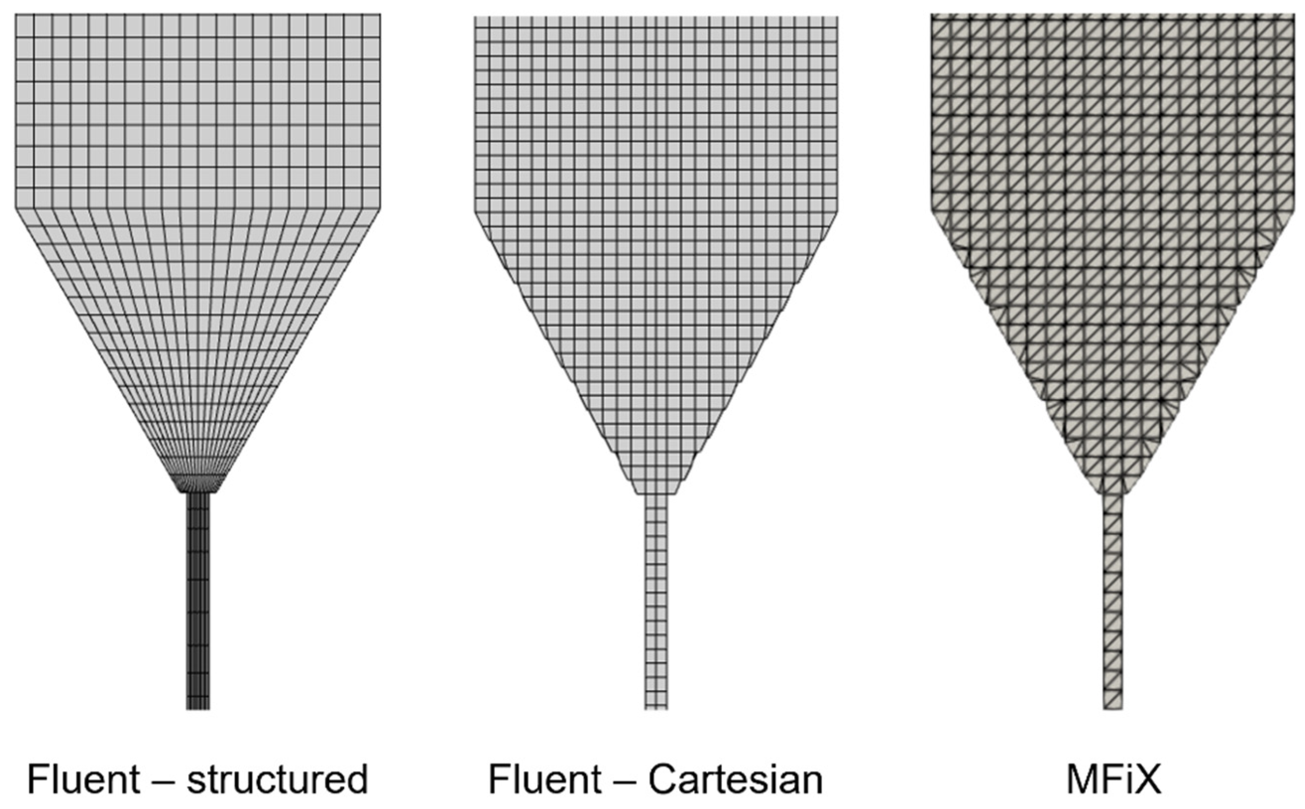
The simulations are based on the experimental work by Zhao et al. [14], which has already been used by several authors to validate CFD-DEM simulations. The unit is a pseudo-2D spouted bed, whose dimensions are summarised in Table 1. The comparison is performed employing the time-averaged profile of the particles’ vertical velocity along the central axis of the spouted bed.

2.2.2. Mesh

The discretisation of the geometry is often a critical aspect in CFD-DEM simulations. In general, one should always search for a compromise so as to obtain a satisfying description of the fluid phase without attaining unrealistic values of the porosity. Specific research has shown that a ratio between the cell and particle sizes of about 4 is the best choice [39], although sometimes even smaller values are successfully employed [40].
The process of creating the computational grid notably differs between Fluent and MFiX. For Fluent, the mesh must be generated externally. The most common option is to generate it with the program Ansys Meshing, which has a wide variety of functionalities to create very different grids. Conversely, the MFiX mesh must be specified within the program, and only a Cartesian cut-cell algorithm [41] can be employed. Since MFiX does not support importing an external mesh, and the meshes generated in MFiX are incompatible with Fluent, it was not possible to employ identical grids for the simulations.
In a previous analysis performed with Fluent [33], the best performing mesh was found to be a structured one with 3 cells along the depth, 62 along the height and 20 along the width (12 in the tube), with an average cell-to-particle size ratio of about 4 in the parallelepipedal part. Such a grid is employed in this work as well, but to make a better comparison with MFiX a Cartesian grid was also created and tested. An unstructured grid was also preliminarily tested but was discarded due to its clearly worse results. The MFiX grid is instead a Cartesian grid with 3 cells along the depth, 65 along the height and 19 along the width. The grid-to-particle size ratio is 4 along the width and height, and 2.5 along the depth. Significantly finer grids prevented the MFiX solver from reaching convergence. The three employed grids are shown in Figure 1.
As Figure 1 clearly shows, the Cartesian grids allow a more regular cell volume and distribution, but do not offer a detailed description of the fluid phase in certain parts, such as near the inlet. This is instead achieved through the structured grid, but at the expense of having several cells whose size approaches that of particles. To avoid numerical instabilities and unphysical porosity values, this grid can only be employed together with an averaging procedure that is discussed below.

2.2.3. Simulation Setup

The simulations regarded a case with an initial bed height of 0.1 m, and an inlet velocity of 26.68 m/s. The parameters employed in the simulations are summarised in Table 2. It shall be noted that in Fluent it is possible to input only a single value of the collision parameters per each collision pair, whereas in MFiX different values for the normal and tangential collision parameters may selected. In this work, we employed the standard values of 2/7 and 1/2 for the ratios between the normal and tangential values of the spring constant and restitution coefficient.
Both Fluent and MFiX allow for reducing the number of particles by lumping several of them in a larger “parcel”; this approach is usually known as “coarse-graining” [42,43]. As the number of involved particles is already quite low, this procedure was not employed here. It should also be noted that using larger parcels requires enlarging the mesh as well.
In MFiX, the particle time step is automatically calculated by the program as 1/50 of the minimum collision time. In the current setup, this procedure yielded a value of about 4.44·10−6 s. The same value was also selected in Fluent for the sake of similarity, although previously a larger value had been successfully used [33]. For the CFD calculations, MFIX utilises an adaptive time step. In this work, it could vary between 10−7 and 10−3 s, although values close to the upper boundary were almost always used by the program after the first few time steps. In Fluent, the CFD time step was instead set to 10−4 s.
The simulations were run on the 21.2.0 version of Fluent, which is incorporated in the 2021R2 release of Ansys. For MFiX, the 21.1.4 version was employed. The simulations were run on Windows 10 on a PC equipped with an Intel(R) Xeon(R) Gold 5218 processor (produced by Intel, Santa Clara, CA, USA), with 16 cores.

2.2.4. Particle Data Averaging

When the size of the grid cells approaches that of particles, numerical instability or unphysical results may appear. To avoid these, CFD-DEM may take advantage of averaging algorithms that distribute the effect of the presence of a particle to nearby cells. When these methods are not employed, the presence of a particle is only taken into account in the cell in which its centre lies, which can be especially inadequate when a particle lies on the border between two or more cells.
For this purpose, Fluent employs a so-called “node-based averaging” algorithm, which is based on a Gaussian function. This algorithm was employed in all simulations, since it was the only way to achieve convergence. In MFiX, two interpolation schemes can be employed: one based on the grid size, and one based on a user-specified interpolation width, which is recommended to be set equal to the particle size. The latter was employed in the simulations, although an analysis of the results showed the effects of its inclusion were rather negligible.

2.2.5. Result Extraction and Post Processing

Extracting and analysing the results is a key task in numerical simulation. Although Fluent offers more in-built functionalities to do this, it is quite difficult to achieve something beyond. For example, Fluent automatically stores several data regarding both fluid and particles, but it is impossible to access the values of most of the forces that act on particles (such as drag and friction). On the other hand, in MFiX the grid values of the particles’ velocity are not accessible by default, but through a modification of the code, these can be saved (one of the most common ways to achieve it is to store them as “reaction rates”). Moreover, most of the data extraction and visualisation cannot be performed within the program itself, but through the command-line tool “postmfix” or through the open-source program Paraview.
Regarding Fluent, the time-averaged data were obtained through the in-built option “data sampling for time statistics”. The algorithm was automatically activated after 1 s of simulation through a command. MFiX offers no in-built option to obtain time-averaged data, but there are two ways to achieve them. One is to create a user-defined subroutine that performs this task, while the other is to do it at the end of the simulation in Paraview, using the saved data. The second method is clearly more immediate, but the output relies on the frequency at which data are saved, whereas through the first method, data can be averaged at each time step. Hence, the first method was employed.

3. Results and Discussion

The performances of the two programs are compared on the basis of the results and computational demands. Finally, their advantages and disadvantages are summarised.

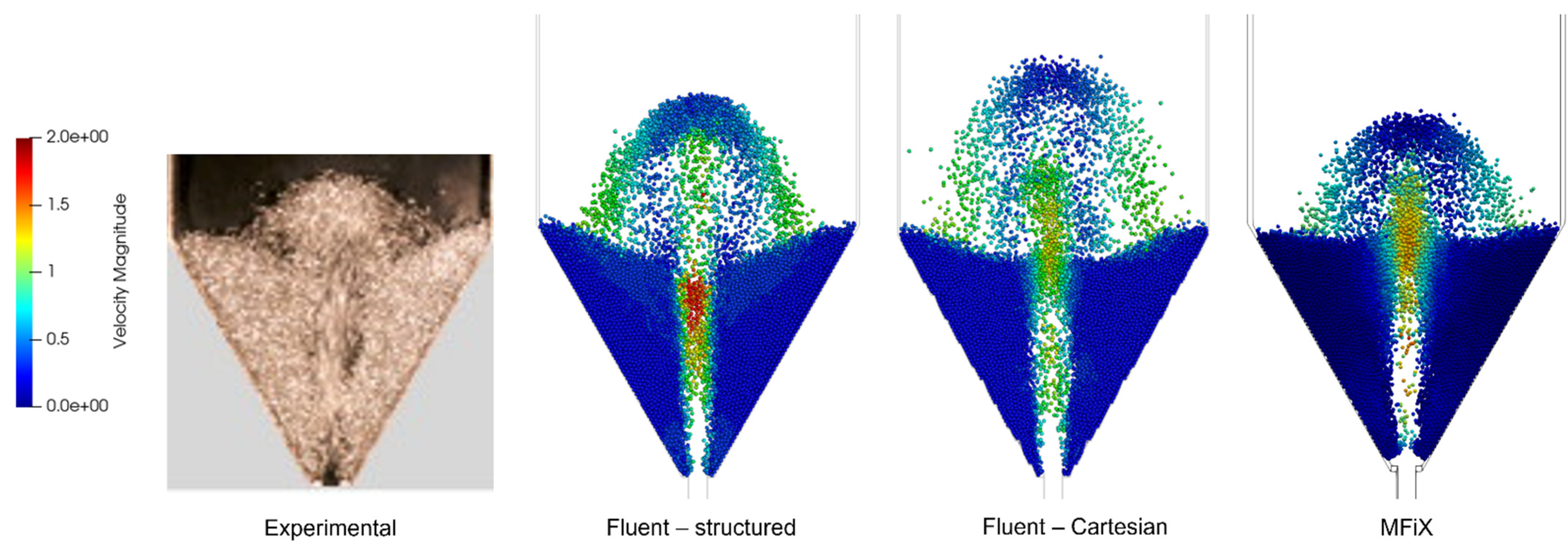
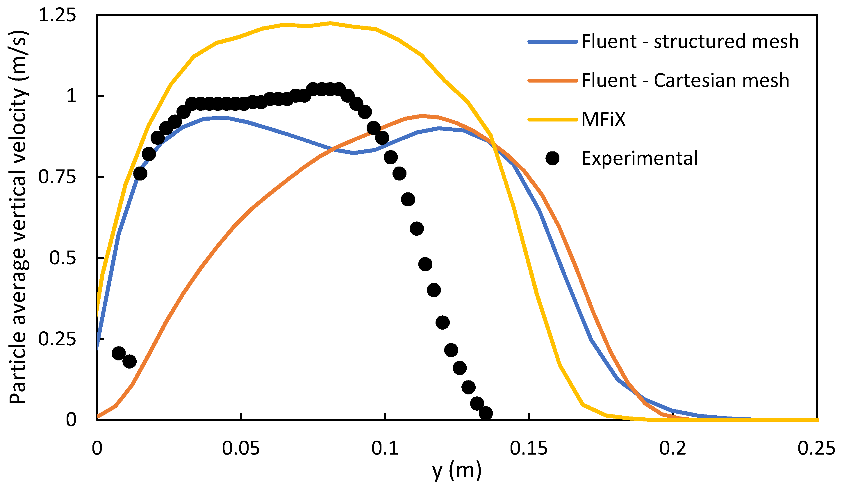
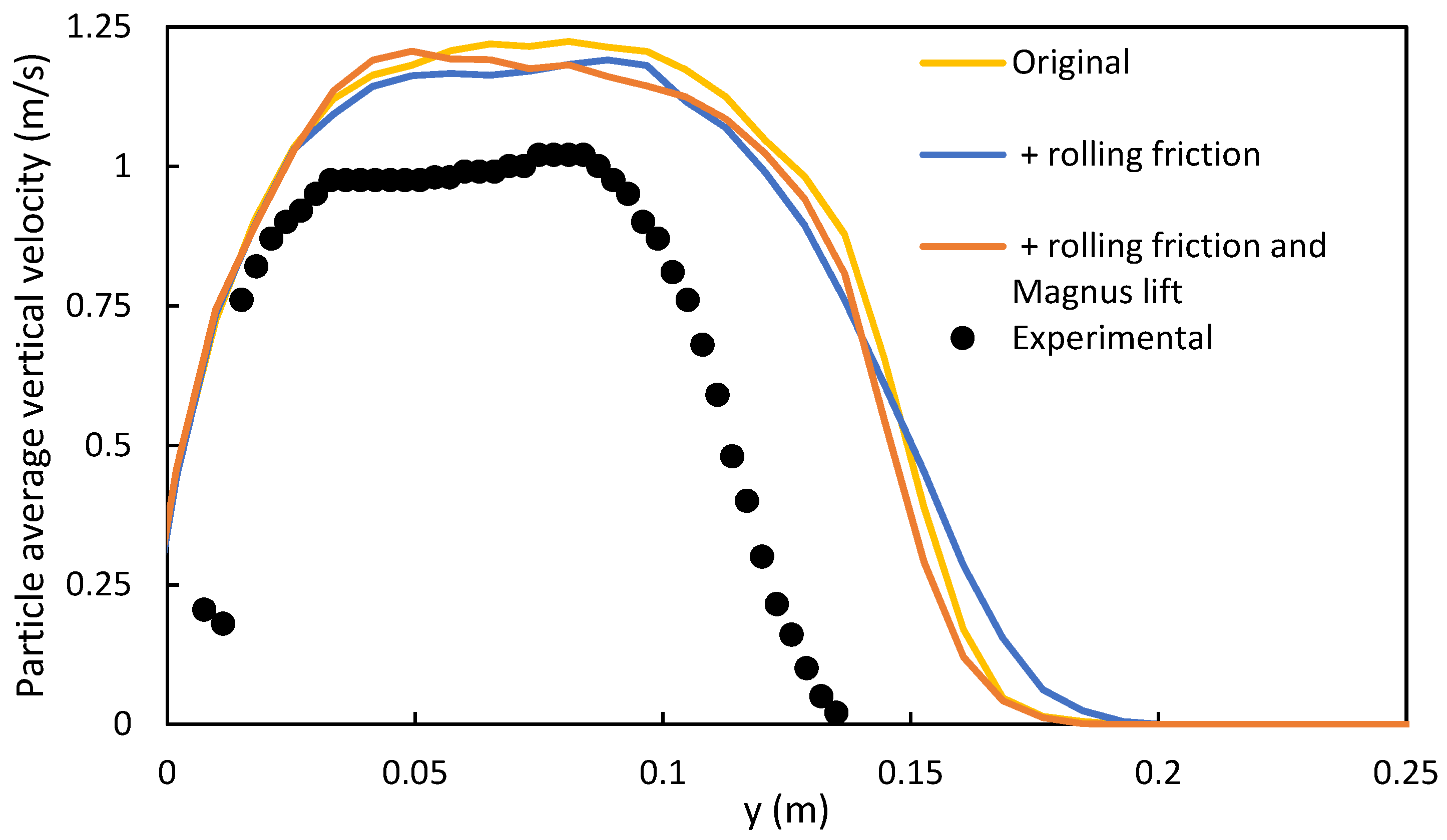
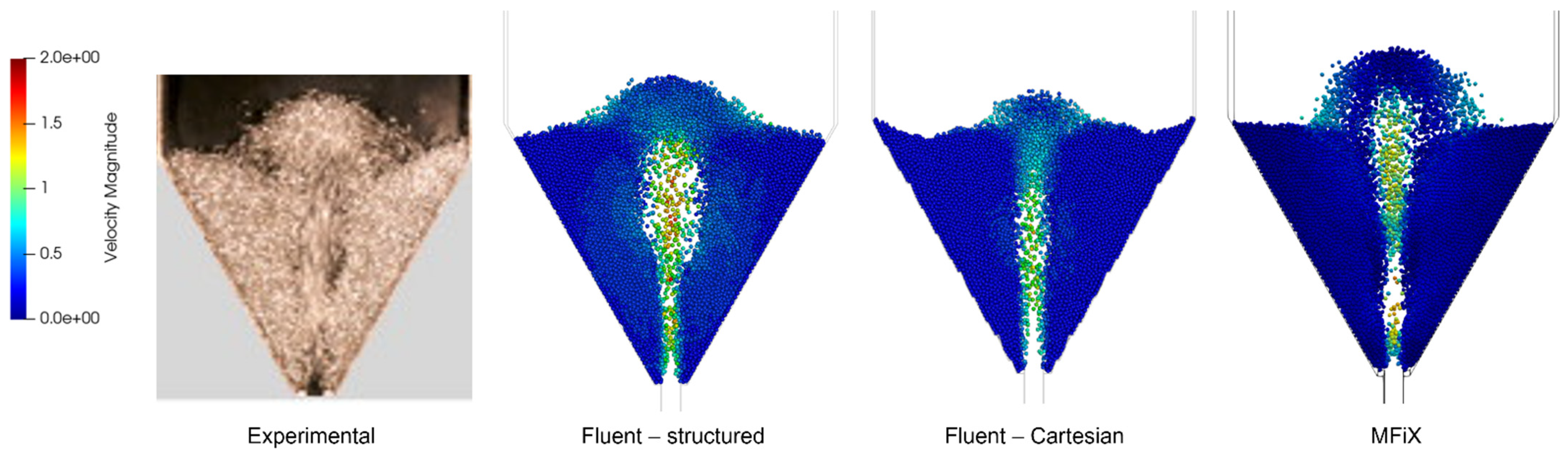
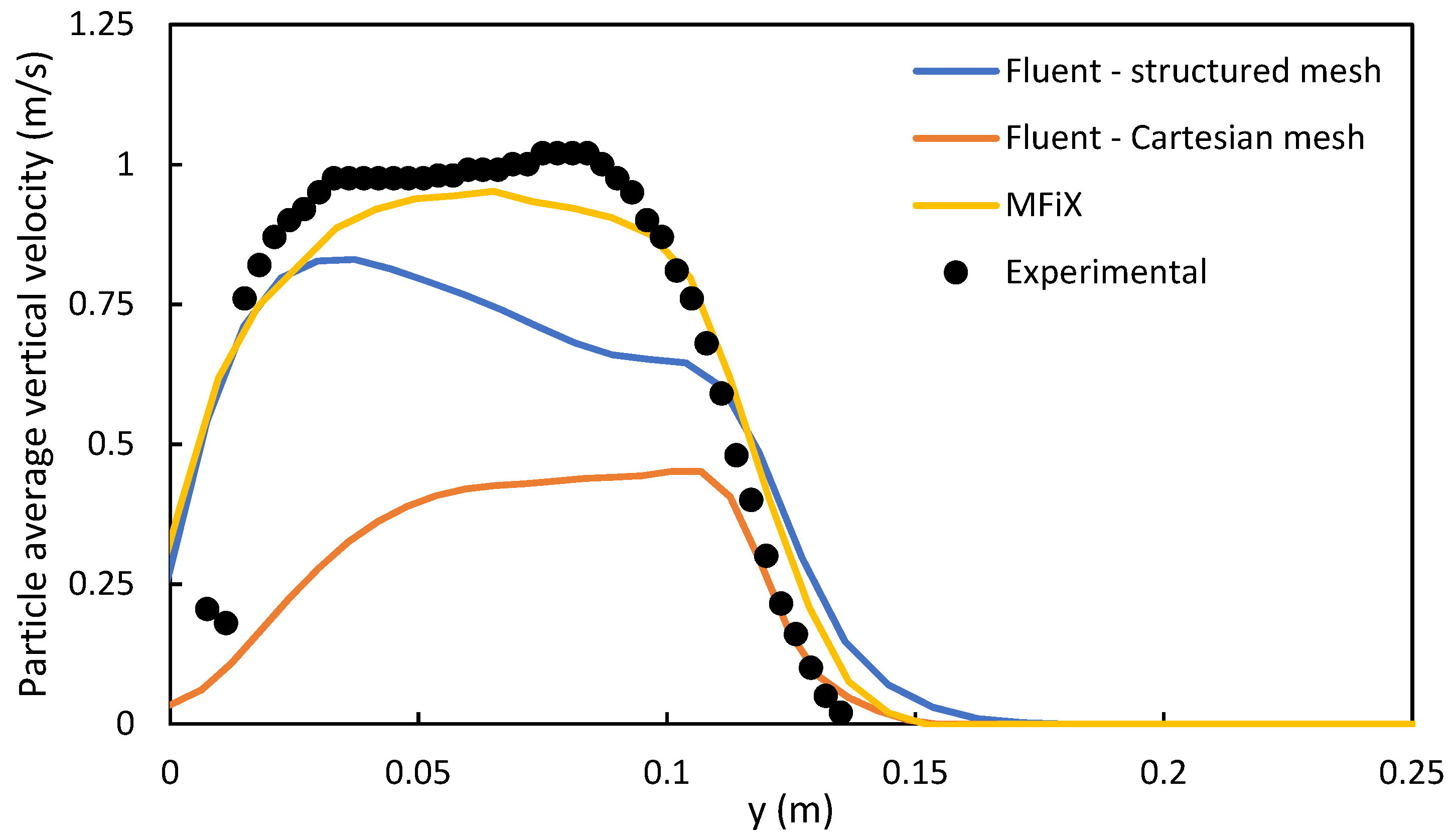
3.1. Comparison of Results

The comparison between the two programs was performed employing specifications that were identical or as similar as possible. As already mentioned, the most outstanding difference lies in the numerical mesh, which cannot be set as identical. Although in a previous analysis a structured mesh appeared to be the best choice, a Cartesian mesh was also tested to employ a more similar grid with respect to MFiX.
The first simulations regarded setups in which we did not employ any user-defined function, to show the standard capabilities of the two programs. The drag is estimated through the Gidaspow model, and the rolling friction and Magnus lift forces are not enabled in MFiX. Figure 2 depicts the results visually. Qualitatively, both programs succeed in providing a good representation of the experimental configuration of the particles. The three typical zones of spouted beds are clearly visible: the spout, which is the central channel in which particles travel rapidly upwards; the fountain, which is the dispersed zone in which particles are scattered while falling back; the annulus, which is the packed zone where particles move slowly downwards and centre-wards.
For a more quantitative assessment, Figure 3 provides the time-averaged vertical profiles of the particles’ vertical velocity. From the plot, both programs do not provide an accurate reproduction of the experimental data. This is not unexpected since, as per a previous work [11], the Gidaspow drag model is rather unsuitable for this setup, even though it was found to be the most chosen in the literature [16]. Fluent seems to moderately underestimate the peak velocity, while it largely overestimates the fountain height (i.e., the highest position reached by particles). Conversely, MFiX overestimates both the peak velocity and the fountain height, but the latter is closer to the experimental value. Another interesting aspect is that both MFiX and Fluent with the structured mesh correctly capture the abrupt acceleration that particles experience near the bottom of the bed. Fluent with the Cartesian mesh instead shows a more gradual and less accurate acceleration, with the peak velocity only reached near the end of the spout. This can be explained due to the higher porosity values that a coarser mesh generates, thus yielding a less intense drag effect. Since the Cartesian Fluent mesh and the MFiX mesh are quite similar, and the forces are calculated in a very similar way, this is a strong hint of the differences between the two codes, especially on the numerical side.
The MFiX code, as already stated, does not include rolling friction and Magnus lift, which are selectable in Fluent. Since a previous analysis pointed towards the importance of including the Magnus lift force, and for the sake of higher accuracy, we modified the MFiX code to add both variables to the particles’ force and torque balance. Figure 4 provides the obtained time-averaged profiles of the particles’ vertical velocity. For the rolling friction torque, the results do not appear to be strongly affected, and the velocity values are only marginally lowered. This is in line with the results of the previous analysis, although the reduction appeared to be more marked [33]. In general, particles do not experience very large relative rotational velocities, and thus the values yielded by Equation (13) are not expected to have a huge impact on the particles’ trajectories.
With regard to the Magnus lift force, our implementation of the Rubinow–Keller model also appears to have a rather negligible effect on the results. This, however, contradicts the results of the aforementioned study, which highlighted that the inclusion of the Magnus lift force had a strong impact on the shape of the velocity profiles. This inconsistency points to one of the major limits of Fluent, i.e., the lack of transparency of its code and the impossibility to access the values of some calculated variables. The Magnus lift force can be enabled, but the value of the force can only be inferred by its effects on the particles’ trajectories.
Finally, we repeated the simulations with the Di Felice drag model, with the aim of checking whether the two programs responded analogously to such a modification. In a previous analysis, this drag model appeared to yield the best results in the present configuration. Figure 5 provides the visual results. Qualitatively, the obtained configurations are again all acceptable. The fountain height is noticeably reduced in all cases, becoming more similar to the experimental one.
If we now observe the velocity profiles, reported in Figure 6, we notice that the one obtained with MFiX is almost identical to the experimental one, thus clearly representing the best choice. The profile obtained with the structured mesh in Fluent is again better than the Gidaspow case, but the peak velocity is quite underestimated, whereas the one obtained with the Cartesian mesh yields a good reproduction of the fountain height, but a very poor one of the overall velocity. In general, both programs confirm that the Di Felice model, compared to the Gidaspow one, results in a markedly lower drag force in this configuration, thus lowering the particle velocity and fountain height. It thus is further confirmed to be the best choice to simulate the current setup. These results also confirm the accuracy of the computational frameworks, since the equation of the Di Felice model generally yields lower values than the Gidaspow model [11].

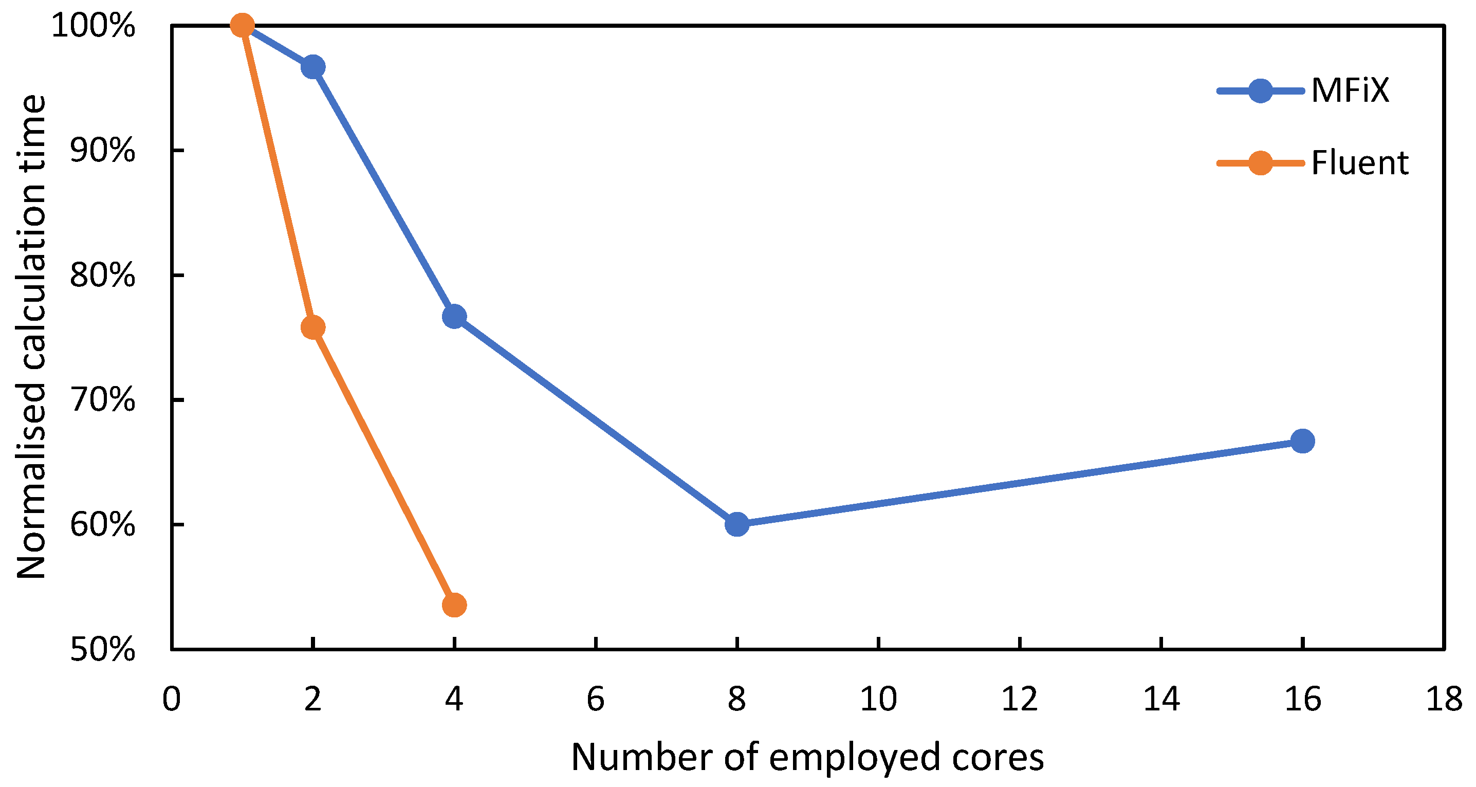
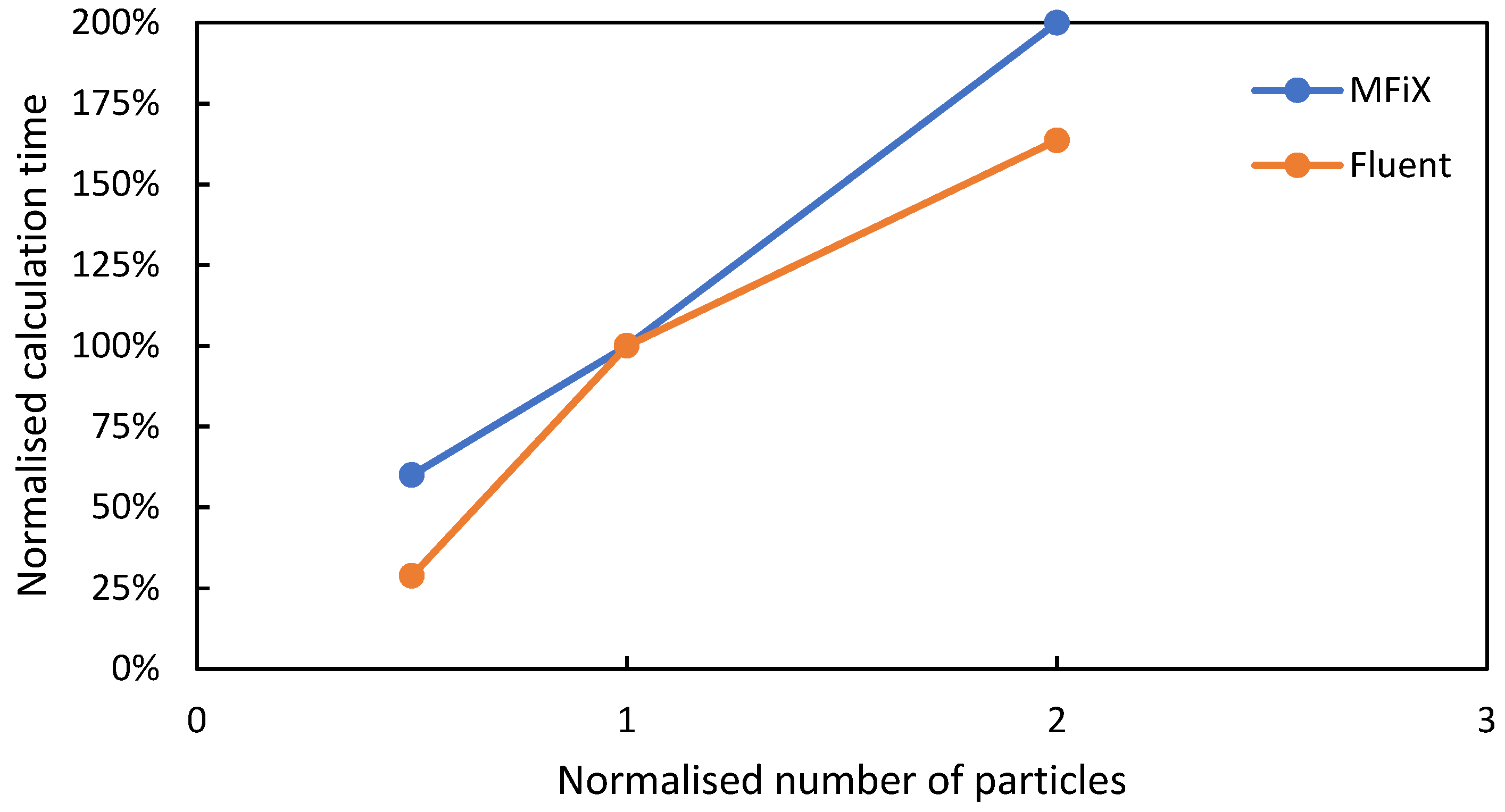
3.2. Comparison of Calculation Time

Accuracy is an indispensable factor when choosing a simulation program. However, given how CFD-DEM simulations can be demanding from a computational point of view, the computational demand should never be overlooked. Regarding this, our observations point largely in favour of MFiX. To perform the simulations described in the previous section, which featured nearly identical setups and numerical parameters, MFiX required about 60 min of calculation per 1 s of simulation, whereas Fluent needed about 1050 min. Given that the large majority of the calculation time was employed by both programs to perform the DEM calculations, it may be concluded that the particle-related algorithm of MFiX is more efficient. It should be noted that, in a previous work, this same spouted bed was simulated in Fluent with a tenfold larger DEM time step on a less performing PC, without any significant variation in the results. In that case, the required simulation time was about 200 min per 1 s.
CFD simulations can be notably sped up by employing parallel computing, which in some cases is mandatory to achieve the desired results within reasonable time scales. Both programs allow employing this functionality, and especially for MFiX several details about its implementation are available in the literature [44,45]. It needs to be noted that parallel computation was not supported in MFiX for Windows before of version 21.3, with Windows users having to employ a virtual machine to perform such calculations. However, any number of cores may be used. Conversely, Fluent can easily be run in parallel on Windows, but the student licence currently does not allow employing more than 4 cores. Figure 7 compares the normalised computation time per 1 s of simulation that was needed in Fluent and MFiX when employing different numbers of cores. The normalised computation time is calculated by dividing the calculation time by the one required by a standard simulation in serial mode, with either Fluent or MFiX. From the plot, it is clear that the parallelisation algorithm of Fluent is more efficient, enabling a greater reduction in the computational time when employing the same number of cores. To achieve the same relative timesaving with MFiX, roughly double the number of cores is required. Moreover, it can also be seen that an excessive number of cores does not provide any advantage: most likely, for such a relatively small-scale problem, the communication becomes too heavy to bring any advantage. In absolute terms, however, MFiX is still the winner, reaching a minimum of 36 min/s against the 562 of Fluent.
CFD-DEM simulations are also strongly affected by the number of particles. To achieve a rough idea of how the two programs respond when this variable changes, we ran identical simulations with halved and doubled amounts of particles. Figure 8 depicts the results in a normalised fashion. The two programs appear to respond quite similarly to the number of particle variation, with Fluent being slightly more efficient. If this trend continued for larger numbers of particles, at a certain point the two programs would show very similar performances, but of course this is not something that can be confirmed through the current investigation.

3.3. Summary of Advantages and Disadvantages

The previous results have shown that both programs have advantages and disadvantages. For the specific case of this spouted bed, MFiX clearly appears as the superior choice, providing better results within a shorter timescale, but for a different application, other considerations may apply. In any case, both programs are powerful and versatile tools that can be employed to perform CFD-DEM simulations. Table 3 sums up a point-by-point comparison of the two programs.

4. Conclusions

A pseudo-2D spouted bed was simulated through the CFD-DEM approach, comparing the performance of the commercial program Ansys Fluent and the open-source program MFiX. Both programs can provide acceptable qualitative predictions when employing standard settings. If the Di Felice drag model is applied, MFiX yields better results and provides a very good quantitative reproduction of the experimental particle velocity profile. Moreover, despite employing similar mesh and time steps and the same number of particles, MFiX is about 17 times faster. However, Fluent seems to respond slightly more efficiently to an increase in the particle number and appears to have better parallelisation functionalities. The Magnus lift force is also implemented in MFiX, and the results do not change significantly, which is very different from what was observed in Fluent.

Author Contributions

Conceptualization, data curation, formal analysis, methodology, software, visualization, writing—original draft: F.M.; funding acquisition, supervision, writing—review and editing: R.D.F. All authors have read and agreed to the published version of the manuscript.

Funding

Filippo Marchelli’s research grant was co-funded by the Liguria Region under the Programma Operativo Por FSE Regione Liguria 2014–2020 (code RLOF18ASSRIC/42/1).
Fluids 06 00382 i001

Institutional Review Board Statement

Not applicable.

Informed Consent Statement

Not applicable.

Data Availability Statement

The experimental data employed for the validation are published and available at doi.org/10.1016/j.powtec.2007.11.044 (last accessed on 18 October 2021, published by Elsevier, Amsterdam, Netherlands). The data produced by the simulations are available in the article and can be provided by the corresponding author in higher detail.

Conflicts of Interest

The authors declare no conflict of interest. The funders had no role in the design of the study; in the collection, analyses, or interpretation of data; in the writing of the manuscript, or in the decision to publish the results.

References

  1. Kennedy, D. What Don’t We Know? Science 2005, 309, 75. [Google Scholar] [CrossRef] [Green Version]
  2. Van der Hoef, M.A.; Ye, M.; van Sint Annaland, M.; Andrews, A.T.; Sundaresan, S.; Kuipers, J.A.M. Multiscale Modeling of Gas-Fluidized Beds; Elsevier: Amsterdam, The Netherlands, 2006; Volume 31, ISBN 0120085313. [Google Scholar]
  3. Ngo, S.I.; Lim, Y.-I. Multiscale Eulerian CFD of Chemical Processes: A Review. ChemEngineering 2020, 4, 23. [Google Scholar] [CrossRef] [Green Version]
  4. Kieckhefen, P.; Pietsch, S.; Dosta, M.; Heinrich, S. Possibilities and Limits of Computational Fluid Dynamics–Discrete Element Method Simulations in Process Engineering: A Review of Recent Advancements and Future Trends. Annu. Rev. Chem. Biomol. Eng. 2020, 11, 397–422. [Google Scholar] [CrossRef] [Green Version]
  5. Cundall, P.A.; Strack, O.D.L. A discrete numerical model for granular assemblies. Géotechnique 1979, 29, 47–65. [Google Scholar] [CrossRef]
  6. Tsuji, Y.; Tanaka, T.; Ishida, T. Lagrangian numerical simulation of plug flow of cohesionless particles in a horizontal pipe. Powder Technol. 1992, 71, 239–250. [Google Scholar] [CrossRef]
  7. Moliner, C.; Marchelli, F.; Spanachi, N.; Martinez-Felipe, A.; Bosio, B.; Arato, E. CFD simulation of a spouted bed: Comparison between the Discrete Element Method (DEM) and the Two Fluid Model (TFM). Chem. Eng. J. 2019, 377, 120466. [Google Scholar] [CrossRef] [Green Version]
  8. Ostermeier, P.; DeYoung, S.; Vandersickel, A.; Gleis, S.; Spliethoff, H. Comprehensive investigation and comparison of TFM, DenseDPM and CFD-DEM for dense fluidized beds. Chem. Eng. Sci. 2019, 196, 291–309. [Google Scholar] [CrossRef]
  9. Lungu, M.; Siame, J.; Mukosha, L. Comparison of CFD-DEM and TFM approaches for the simulation of the small scale challenge problem 1. Powder Technol. 2021, 378, 85–103. [Google Scholar] [CrossRef]
  10. Liu, D.; Bu, C.; Chen, X. Development and test of CFD–DEM model for complex geometry: A coupling algorithm for Fluent and DEM. Comput. Chem. Eng. 2013, 58, 260–268. [Google Scholar] [CrossRef]
  11. Marchelli, F.; Hou, Q.; Bosio, B.; Arato, E.; Yu, A. Comparison of different drag models in CFD-DEM simulations of spouted beds. Powder Technol. 2020, 360, 1253–1270. [Google Scholar] [CrossRef]
  12. Li, J.; Campbell, G.M.; Mujumdar, A.S. Discrete Modeling and Suggested Measurement of Heat Transfer in Gas–Solids Flows. Dry. Technol. 2003, 21, 979–994. [Google Scholar] [CrossRef]
  13. Albano, A.; le Guillou, E.; Danzé, A.; Moulitsas, I.; Sahputra, I.H.; Rahmat, A.; Duque-Daza, C.A.; Shang, X.; Ching Ng, K.; Ariane, M.; et al. How to Modify LAMMPS: From the Prospective of a Particle Method Researcher. ChemEngineering 2021, 5, 30. [Google Scholar] [CrossRef]
  14. Zhao, X.-L.L.; Li, S.-Q.Q.; Liu, G.-Q.Q.; Yao, Q.; Marshall, J.-S.S. DEM simulation of the particle dynamics in two-dimensional spouted beds. Powder Technol. 2008, 184, 205–213. [Google Scholar] [CrossRef]
  15. Geldart, D. Types of gas fluidization. Powder Technol. 1973, 7, 285–292. [Google Scholar] [CrossRef]
  16. Moliner, C.; Marchelli, F.; Bosio, B.; Arato, E. Modelling of spouted and spout-fluid beds: Key for their successful scale up. Energies 2017, 10, 1729. [Google Scholar] [CrossRef] [Green Version]
  17. Herzog, N.; Schreiber, M.; Egbers, C.; Krautz, H.J. A comparative study of different CFD-codes for numerical simulation of gas–solid fluidized bed hydrodynamics. Comput. Chem. Eng. 2012, 39, 41–46. [Google Scholar] [CrossRef]
  18. Venier, C.M.; Urrutia, A.R.; Capossio, J.P.; Baeyens, J.; Mazza, G. Comparing ANSYS Fluent ® and OpenFOAM ® simulations of Geldart A, B and D bubbling fluidized bed hydrodynamics. Int. J. Numer. Methods Heat Fluid Flow 2019, 30, 93–118. [Google Scholar] [CrossRef]
  19. Marchelli, F.; Moliner, C.; Curti, M.; Bosio, B.; Arato, E. CFD-DEM simulations of a continuous square-based spouted bed and evaluation of the solids residence time distribution. Powder Technol. 2020, 366, 840–858. [Google Scholar] [CrossRef]
  20. Garg, R.; Galvin, J.; Li, T.; Pannala, S. Open-source MFIX-DEM software for gas-solids flows: Part I-Verification studies. Powder Technol. 2012, 220, 122–137. [Google Scholar] [CrossRef]
  21. ANSYS ANSYS Fluent User Guide; ANSYS: Canonsburg, PA, USA, 2019.
  22. ANSYS ANSYS Fluent Theory Guide; ANSYS: Canonsburg, PA, USA, 2019.
  23. Syamlal, M.; Rogers, W.; O‘Brien, T.J. MFIX Documentation Theory Guide; Department of Energy: Oak Ridge, TN, USA, 1993; Volume 1004.
  24. Chu, K.W.; Kuang, S.B.; Zhou, Z.Y.; Yu, A.B. Model A vs. Model B in the modelling of particle-fluid flow. Powder Technol. 2018, 329, 47–54. [Google Scholar] [CrossRef]
  25. Marchelli, F.; Di Felice, R. A Discrete Element Method Study of Solids Stress in Cylindrical Columns Using MFiX. Processes 2020, 9, 60. [Google Scholar] [CrossRef]
  26. Launder, B.E.; Spalding, D.B. The numerical computation of turbulent flows. Comput. Methods Appl. Mech. Eng. 1974, 3, 269–289. [Google Scholar] [CrossRef]
  27. Weaver, D.S.; Mišković, S. A Study of RANS Turbulence Models in Fully Turbulent Jets: A Perspective for CFD-DEM Simulations. Fluids 2021, 6, 271. [Google Scholar] [CrossRef]
  28. Gidaspow, D. Multiphase Flow and Fluidization: Continuum and Kinetic Theory Descriptions; Academic Press: Cambridge, MA, USA, 1994. [Google Scholar]
  29. Di Felice, R. The voidage function for fluid-particle interaction systems. Int. J. Multiph. Flow 1994, 20, 153–159. [Google Scholar] [CrossRef]
  30. Ergun, S. Fluid flow through packed columns. Chem. Eng. Prog. 1952, 48, 89–94. [Google Scholar]
  31. Wen, C.Y.; Yu, Y.H. Mechanics of Fluidization. Chem. Eng. Prog. Symp. Ser. 1966, 162, 100–111. [Google Scholar]
  32. Rong, L.W.; Dong, K.J.; Yu, A.B. Lattice-Boltzmann simulation of fluid flow through packed beds of uniform spheres: Effect of porosity. Chem. Eng. Sci. 2013, 99, 44–58. [Google Scholar] [CrossRef]
  33. Marchelli, F.; Moliner, C.; Bosio, B.; Arato, E. A CFD-DEM sensitivity analysis: The case of a pseudo-2D spouted bed. Powder Technol. 2019, 353, 409–425. [Google Scholar] [CrossRef]
  34. Liu, R.-J.; Xiao, R.; Ye, M.; Liu, Z. Analysis of particle rotation in fluidized bed by use of discrete particle model. Adv. Powder Technol. 2018, 29, 1655–1663. [Google Scholar] [CrossRef]
  35. Rubinow, S.I.; Keller, J.B. The transverse force on a spinning sphere moving in a viscous fluid. J. Fluid Mech. 1961, 11, 447. [Google Scholar] [CrossRef]
  36. Marchelli, F.; Di Felice, R. On the influence of contact models on friction forces in discrete element method simulations. Chem. Eng. Trans. 2021, 86, 811–816. [Google Scholar]
  37. Ai, J.; Chen, J.F.; Rotter, J.M.; Ooi, J.Y. Assessment of rolling resistance models in discrete element simulations. Powder Technol. 2011, 206, 269–282. [Google Scholar] [CrossRef]
  38. Zhou, Y.C.; Wright, B.D.; Yang, R.Y.; Xu, B.H.; Yu, A.B. Rolling friction in the dynamic simulation of sandpile formation. Phys. A Stat. Mech. Its Appl. 1999, 269, 536–553. [Google Scholar] [CrossRef]
  39. Boyce, C.M.; Holland, D.J.; Scott, S.A.; Dennis, J.S. Limitations on Fluid Grid Sizing for Using Volume-Averaged Fluid Equations in Discrete Element Models of Fluidized Beds. Ind. Eng. Chem. Res. 2015, 54, 10684–10697. [Google Scholar] [CrossRef]
  40. Hamidouche, Z.; Dufresne, Y.; Pierson, J.-L.; Brahem, R.; Lartigue, G.; Moureau, V. DEM/CFD Simulations of a Pseudo-2D Fluidized Bed: Comparison with Experiments. Fluids 2019, 4, 51. [Google Scholar] [CrossRef] [Green Version]
  41. Berger, M. Cut Cells: Meshes and Solvers. In Handbook of Numerical Analysis; Elsevier: Amsterdam, The Netherlands, 2017; Volume 18, pp. 1–22. [Google Scholar]
  42. Chu, K.W.; Chen, J.; Wang, B.; Yu, A.B.; Vince, A.; Barnett, G.D.; Barnett, P.J. Understand solids loading effects in a dense medium cyclone: Effect of particle size by a CFD-DEM method. Powder Technol. 2017, 320, 594–609. [Google Scholar] [CrossRef]
  43. Di Renzo, A.; Napolitano, E.; Di Maio, F. Coarse-Grain DEM Modelling in Fluidized Bed Simulation: A Review. Processes 2021, 9, 279. [Google Scholar] [CrossRef]
  44. Gopalakrishnan, P.; Tafti, D. Development of parallel DEM for the open source code MFIX. Powder Technol. 2013, 235, 33–41. [Google Scholar] [CrossRef]
  45. Liu, H.; Tafti, D.K.; Li, T. Hybrid parallelism in MFIX CFD-DEM using OpenMP. Powder Technol. 2014, 259, 22–29. [Google Scholar] [CrossRef]
Figure 1. The three employed meshes. Please note that the upper portion of the mesh is not shown as it is not relevant for the comparison, and that the diagonals of the squares in the MFiX mesh are only aesthetic.
Fluids 06 00382 g001
Figure 2. Configuration of the particles after 2 s of simulation with the Gidaspow drag model. The particles are coloured according to their velocity magnitude. Experimental snapshot reprinted from [14], Copyright (2008), with permission from Elsevier.
Fluids 06 00382 g002
Figure 3. Time-averaged vertical profiles of the particles’ vertical velocity when employing the Gidaspow drag model.
Fluids 06 00382 g003
Figure 4. Time-averaged vertical profiles of the particles’ vertical velocity in MFiX, including additional forces.
Fluids 06 00382 g004
Figure 5. Configuration of the particles after 2 s of simulation with the Di Felice drag model. The particles are coloured according to their velocity magnitude. Experimental snapshot reprinted from [14]. Copyright 2008 Elsevier.
Fluids 06 00382 g005
Figure 6. Time-averaged vertical profiles of the particles’ vertical velocity when employing the Di Felice drag model.
Fluids 06 00382 g006
Figure 7. Normalised calculation time upon employing a different number of cores.
Fluids 06 00382 g007
Figure 8. Normalised calculation time upon varying the total number of particles.
Fluids 06 00382 g008
Table 1. Dimensions of the geometry.
VariableValue
Inlet width0.9 cm
Bottom width1.5 cm
Column width15.2 cm
Column depth1.5 cm
Base angle60°
Height of the inclined part11.9 cm
Total height60 cm
Table 2. Parameters employed in the simulations.
VariableValue
Spring constant1000 N/m
Restitution coefficient0.9
Friction coefficient0.3
Rolling friction coefficient0.03
Air density1.225 kg/m3
Air dynamic viscosity1.7894·10−5 Pa·s
Particle density2380 kg/m3
Particle diameter2.033 mm
Total number of particles15,990
Table 3. Point-by-point comparison of Ansys Fluent and MFiX applied to CFD-DEM.
Ansys FluentMFiX
CostCommercial program, a free student licence with limitations is available.Open-source program, entirely free.
GUIBoth programs are equipped with a user-friendly GUI.
Geometry and meshAnsys programs provide numerous options to generate geometry and mesh.The geometry can be created in MFiX or imported, but only Cartesian cut-cell meshes can be employed. This may be a limiting factor for some geometries.
CFD-DEM methodologyAvailable for spherical particles, including coarse-graining. It is also possible to include lift forces, rolling friction torque and other forces.Available for spherical particles, including coarse-graining. Lift forces and rolling friction torque are not included in the standard version of the code.
Code visibilityThe code is not accessible by the user.The code is completely transparent to the user.
PersonalisationUser-defined functions (written in C) allow some level of personalisation, but some variables (such as contact forces) cannot be modified. The code (written in Fortran) is entirely editable by the user.
Results visualisation and analysisNumerous and flexible options are available. However, some variables (such as the drag force) cannot be accessed.The standard options are more limited, but anything can be accessed by editing the code. Paraview is often needed to analyse and visualise the results.
CPU costFor the present application, it is about 17.5 times larger than with MFiX. However, it seems to be less sensitive to increases in the number of particles.For the present application, it is about 17.5 times smaller than with Fluent. However, it seems to be more sensitive to increases of the number of particles.
ParallelisationWith the same number of cores, the relative speed-up is larger than with MFiX. The student licence does not allow more than 4 cores.With the same number of cores, the relative speed-up is smaller than with Fluent.
Available materialThe user and theory guide are very detailed, and the interface is clear, but the material related to the CFD-DEM methodology is scarce.Several tutorials on the CFD-DEM methodology are available, but learning how to modify the code can require some effort.
Other applicationsThe program has many options and can be employed for a variety of applications in different fields.The program is specifically aimed at situations involving granular materials. It allows employing other related methodologies (TFM, MP-PIC, DEM).
Publisher’s Note: MDPI stays neutral with regard to jurisdictional claims in published maps and institutional affiliations.

